2 Experimental procedure and free-stream characteristics

The experimental database used in the present study is a combination of the data acquired by Dogan et al. (Reference Dogan, Hanson and Ganapathisubramani2016, Reference Dogan, Hearst and Ganapathisubramani2017), supplemented with some new test cases. The experimental apparatus and acquisition protocol used for the new cases is the same as described by Dogan et al. (Reference Dogan, Hearst and Ganapathisubramani2017). In short, a rake of four single-wire hot-wires was traversed through a TBL subjected to FST in the $0.9~\text{m}\times 0.6~\text{m}\times 4.5~\text{m}$ suction wind tunnel at the University of Southampton. The TBL was formed over a false-floor/boundary layer plate placed in the wind tunnel and was passively tripped. The FST was generated with an active grid placed at the inlet of the test section. Measurements were performed at a fixed position $43M$ downstream of the grid and $Re_{\unicode[STIX]{x1D703}}>2000$ for all measurements making the influence of the tripping mechanism negligible (Schlatter & Örlü Reference Schlatter and Örlü2012). The set-up of Dogan et al. (Reference Dogan, Hanson and Ganapathisubramani2016) was similar to the above, except that only a single wire was traversed through the TBL with another fixed in the free stream. See Dogan et al. (Reference Dogan, Hanson and Ganapathisubramani2016, Reference Dogan, Hearst and Ganapathisubramani2017) for more details on the experimental set-ups.

Table 1.

Flow parameters for all test cases. The dagger ( $\dagger$ ) identifies test cases acquired with the set-up of Dogan et al. (Reference Dogan, Hearst and Ganapathisubramani2017); all other test cases are from Dogan et al. (Reference Dogan, Hanson and Ganapathisubramani2016). The double-dagger ( $\ddagger$ ) indicates the test performed in ‘fully random’ mode; all other tests were conducted in ‘synchronous’ mode.

The test cases used in the present study are summarised in table 1. They are labelled with letters in order of increasing $u_{\infty }^{\prime }/U_{\infty }$ . Additionally, they are separated into groups where free-stream turbulence intensity ( $u_{\infty }^{\prime }/U_{\infty }$ ) and the Taylor microscale Reynolds number ( $Re_{\unicode[STIX]{x1D706},\infty }=u_{\infty }^{\prime }\unicode[STIX]{x1D706}_{\infty }/\unicode[STIX]{x1D708}$ ) are approximately matched; the Taylor microscale was estimated assuming local isotropy in the free stream,

(2.1) $$\begin{eqnarray}\unicode[STIX]{x1D706}^{2}=\frac{\left\langle u^{2}\right\rangle }{\left\langle (\unicode[STIX]{x2202}u/\unicode[STIX]{x2202}x)^{2}\right\rangle }.\end{eqnarray}$$

Streamwise velocity gradients were approximated with Taylor’s frozen flow hypothesis ( $\unicode[STIX]{x2202}(\cdot )/\unicode[STIX]{x2202}t=U\unicode[STIX]{x2202}(\cdot )/\unicode[STIX]{x2202}x$ ) and a sixth-order centred-difference scheme; the latter has been shown to balance the need for spatio-temporal resolution while limiting high-frequency noise (Hearst et al. Reference Hearst, Buxton, Ganapathisubramani and Lavoie2012). In table 1, the integral length scale was estimated from

(2.2) $$\begin{eqnarray}L_{u}=\int _{0}^{r_{0}}\frac{\langle u(x)u(x+r)\rangle }{\left\langle u^{2}\right\rangle }\hspace{2.22198pt}\text{d}r,\end{eqnarray}$$

where $r_{0}$ is the first zero crossing of the autocorrelation. The boundary layer parameters listed in the table ( $\unicode[STIX]{x1D6FF}$ , $U_{\unicode[STIX]{x1D70F}}$ , $\unicode[STIX]{x1D705}$ ) were fitted using the approach of Rodríguez-López, Bruce & Buxton (Reference Rodríguez-López, Bruce and Buxton2015) as modified for FST by Esteban et al. (Reference Esteban, Dogan, Rodríguez-López and Ganapathisubramani2017). Due to the relatively high $Re_{\unicode[STIX]{x1D70F}}$ of the present experiments and the $\ell =1$  mm sensing length of the hot-wire probes, the inner-unit length of the probes was in the range $18\leqslant \ell ^{+}\leqslant 33$ . As such, the variance in the near-wall region was compensated for using the approach of Smits et al. (Reference Smits, Monty, Hultmark, Bailey, Hutchins and Marusic2011). Any differences between the values reported in table 1 and our earlier works are a result of the different fitting process used here and the adjustments for spatial resolution.

The incoming conditions for the various test cases were changed by adjusting the active grid settings as well as the incoming Reynolds number. The grid was operated in one of two modes: ‘synchronous’ or ‘fully random’. In ‘synchronous’ mode, all motors of the grid were updated simultaneously at 1 Hz. In ‘fully random’ mode, updates to each motor of the grid were randomised at intervals between 0.4 and 20 Hz. The actuation velocity of the wings ( $\unicode[STIX]{x1D6FA}$ ) was varied to produce different free-stream conditions. The range of $\unicode[STIX]{x1D6FA}$ is shown for each case in table 1 and was always a top-hat distribution. The chosen test cases were modelled after those of Kang, Chester & Meneveau (Reference Kang, Chester and Meneveau2003), Larssen & Devenport (Reference Larssen and Devenport2011) and Hearst, Gomit & Ganapathisubramani (Reference Hearst, Gomit and Ganapathisubramani2016). Additionally, two different wing geometries were used: solid square wings or wings with holes. Changing the wing geometry has been shown to offset the produced $u_{\infty }^{\prime }/U_{\infty }$ (Thormann & Meneveau Reference Thormann and Meneveau2014; Hearst & Lavoie Reference Hearst and Lavoie2015; Dogan et al. Reference Dogan, Hanson and Ganapathisubramani2016).

Figure 1.

Velocity spectra in the free stream (a) normalised by Taylor scales and (b) in pre-multiplied form. Lightest to darkest lines represent increasing $u_{\infty }^{\prime }/U_{\infty }$ .

The free-stream velocity spectra are shown for all cases in figure 1. In figure 1(a), the spectra are normalised by $\unicode[STIX]{x1D706}$ , which is expected to collapse the spectra in the scaling (or inertial) range as shown. The slope of the nearly two decade long scaling range is close to, but not exactly, $k_{x}^{-5/3}$ ; this agrees with previous active grid studies (Mydlarski & Warhaft Reference Mydlarski and Warhaft1996; Hearst & Lavoie Reference Hearst and Lavoie2015). The same spectra are shown in pre-multiplied form plotted against $\unicode[STIX]{x1D6FF}$ -normalised wavelength ( $\unicode[STIX]{x1D701}_{x}=2\unicode[STIX]{x03C0}/k_{x}$ ) in figure 1(b). As also shown by Dogan et al. (Reference Dogan, Hanson and Ganapathisubramani2016), the peak in the pre-multiplied spectra for all cases is roughly collapsed around $\unicode[STIX]{x1D701}_{x}=10\unicode[STIX]{x1D6FF}$ . Figure 1 highlights two key features of the flow for all cases. First, and not insignificantly, these are relatively high $Re_{\unicode[STIX]{x1D706},\infty }$ FST flows and as such their spectral shape does not significantly vary between cases. This is not a consequence of poor choice of test cases, but rather is a consequence of the governing fluid dynamics that results in a spectrum that may be approximately described by the Richardson–Kolmogorov cascade and cannot be significantly changed. Second, at this evolution distance ( $x/M=43$ ) downstream of the turbulence generation the spectra appear to have all taken on a rough form where their pre-multiplied peak is approximately $10\unicode[STIX]{x1D6FF}$ . Given that $\unicode[STIX]{x1D6FF}$ , $u_{\infty }^{\prime }/U_{\infty }$ and $Re_{\unicode[STIX]{x1D70F}}$ change by factors of 0.5, 2 and 3, respectively, across all cases in table 1, figure 1(b) is highly suggestive that the boundary layer adjusts such that the peak in the pre-multiplied turbulence is at ${\sim}10\unicode[STIX]{x1D6FF}$ and that this not simply a coincidence.

Figure 2.

Pre-multiplied velocity spectra in the free stream for cases (a) G and H, (b) K and M and (c) N and O: (——) cases G, K and N; (— ⋅ —) cases H, M, and O. The bottom panels (d), (e) and (f) show the ratio of the two curves presented in (a), (b) and (c), respectively; $i$ represents the solid line and $j$ represents the dashed line.

Before leaving this section, we draw the reader’s attention to the variation in $L_{u,\infty }$ for the various groups of cases in table 1. The variations in $L_{u,\infty }$ are a result of the changes to the active grid settings. For some groups, the variation in $L_{u,\infty }$ is marginal; however, we draw particular attention to cases G ( $L_{u,\infty }/\unicode[STIX]{x1D6FF}=2.5$ ) and H ( $L_{u,\infty }/\unicode[STIX]{x1D6FF}=1.7$ ) with a 50 % change in integral scale at $u_{\infty }^{\prime }/U_{\infty }\approx 8.1\,\%$ , K ( $L_{u,\infty }/\unicode[STIX]{x1D6FF}=2.8$ ) and M ( $L_{u,\infty }/\unicode[STIX]{x1D6FF}=2.2$ ) with a 20 % change in the integral scale at $u_{\infty }^{\prime }/U_{\infty }=12.0\,\%$ and N ( $L_{u,\infty }/\unicode[STIX]{x1D6FF}=1.6$ ) and O ( $L_{u,\infty }/\unicode[STIX]{x1D6FF}=2.7$ ) with a 65 % change in the integral scale at $u_{\infty }^{\prime }/U_{\infty }\approx 12.3\,\%$ . We note that to achieve the same $u_{\infty }^{\prime }/U_{\infty }$ for G and H, it was necessary to change $U_{\infty }$ marginally; however, the ratio $U_{\infty }/U_{\unicode[STIX]{x1D70F}}=U_{\infty }^{+}$ was approximately the same for both cases.

Figure 3.

Wall-normal profiles of the (a) mean velocity and (b) turbulent fluctuations, both normalised by wall units. See table 1 for symbols. Lightest to darkest symbols represent increasing $u_{\infty }^{\prime }/U_{\infty }$ . Each set of profiles have approximately the same $u_{\infty }^{\prime }/U_{\infty }$ and are offset by $+5$ from one another. In (a) the parameters used for the log-law fit are $\unicode[STIX]{x1D705}=0.39$ and ${\mathcal{B}}=4.3$ , which are taken approximately from Marusic et al. (Reference Marusic, Monty, Hultmark and Smits2013).

The free-stream spectra associated with the identified cases with significant differences in $L_{u,\infty }$ are shown in figure 2(a–c). The area under the two curves in each pair is approximately equal because $u^{\prime }/U_{\unicode[STIX]{x1D70F}}$ is approximately the same for each pair. While the spectra may appear quite similar at first, this is a consequence of the fact that a high $Re_{\unicode[STIX]{x1D706},\infty }$ turbulent field has a relatively fixed shape. The ratio of each set of curves is shown in figure 2(d–f), where the difference between the free-stream flows is more apparent; differences of the order of 20 % exist at the peak in the pre-multiplied spectrum, signifying a significant change in the energy distribution for the same $Re_{\unicode[STIX]{x1D706},\infty }$ .

3 Impact on the boundary layer

Wall-normal profiles of the inner-normalised mean velocity and variance profiles are provided in figure 3. The eye is immediately drawn to the collapse of the flows at a given $u_{\infty }^{\prime }/U_{\infty }$ for both the mean velocity and the variance. The similarity between the curves in the log-law region can be quantified by $\unicode[STIX]{x1D705}$ in table 1, where the difference in $\unicode[STIX]{x1D705}$ between the cases with matched $u_{\infty }^{\prime }/U_{\infty }$ does not exceed 0.03. Furthermore, for a given group of profiles, neither $\unicode[STIX]{x1D6FF}$ nor $U_{\infty }/U_{\unicode[STIX]{x1D70F}}=U_{\infty }^{+}$ changes appreciably. This is particularly significant given that it also holds for the previously identified pairs where $L_{u,\infty }$ changes by up to 65 % and $U_{\infty }$ changes by $1~\text{m}~\text{s}^{-1}$ (representing a 20 % change in bulk energy). This suggests that the bulk characteristics of the TBL subjected to FST are dependent primarily on $u_{\infty }^{\prime }/U_{\infty }$ and $Re_{\unicode[STIX]{x1D706},\infty }$ rather than $L_{u,\infty }$ . This also suggests that figure 11(a) in Dogan et al. (Reference Dogan, Hanson and Ganapathisubramani2016) that shows the variance gain in the boundary layer for different $u_{\infty }^{\prime }/U_{\infty }$ may be sufficient to predict the variance profile given the free-stream turbulence intensity.

Similar characteristics are present in the higher-order statistics for these flows. Namely, the velocity skewness ( $S_{u}=\left\langle u^{3}\right\rangle /\left\langle u^{2}\right\rangle ^{3/2}$ ) and flatness ( 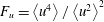$F_{u}=\left\langle u^{4}\right\rangle /\left\langle u^{2}\right\rangle ^{2}$ ) are plotted for each case in figure 4 and demonstrate that for a given $u_{\infty }^{\prime }/U_{\infty }$ these statistics are approximately collapsed near the wall. Some scatter is present in the free stream, particularly visible in the flatness. However, nearer the wall all the curves are collapsed, suggesting the near-wall dynamics are the same. The values of $S_{u}$ and $F_{u}$ both resemble those measured previously by Sharp et al. (Reference Sharp, Neuscamman and Warhaft2009) in a similar set-up. Ultimately, the results demonstrate that at these $Re_{\unicode[STIX]{x1D706},\infty }$ the intermittent discontinuity between the canonical laminar free stream and a turbulent boundary layer does not exist for these flows with FST, but rather the flow takes on the characteristics of approximately homogeneous, isotropic turbulence near the outer regions of the boundary layer. For reference, a Gaussian distribution has $S_{u}=0$ and $F_{u}=3$ .

Figure 4.

Wall-normal profiles of the streamwise velocity (a) skewness and (b) flatness. See table 1 for symbols. Lightest to darkest symbols represent increasing $u_{\infty }^{\prime }/U_{\infty }$ . Each set of profiles have approximately the same $u_{\infty }^{\prime }/U_{\infty }$ and are offset by $+1$ from one another.

Further insight into the resilience of the boundary layer to changes in the FST can be gained by looking at the spectral distribution of energy, viz. the spectrograms, which are shown in figure 5 for the cases with the identified significant changes in $L_{u,\infty }$ . For brevity, we define $\unicode[STIX]{x1D719}^{+}=k_{x}\unicode[STIX]{x1D719}_{u}/U_{\unicode[STIX]{x1D70F}}^{2}$ . All flows exhibit spectral inner and outer peaks, similar to observations made in canonical TBLs (Hutchins & Marusic Reference Hutchins and Marusic2007a ). The inner peak is situated at a wavelength of $\unicode[STIX]{x1D701}_{x}^{+}\approx 1000$ and a wall-normal position of $y^{+}\approx 15$ , for all cases, which is in agreement with previous investigations in canonical TBLs (Hutchins & Marusic Reference Hutchins and Marusic2007a ) and TBLs subjected to FST (Dogan et al. Reference Dogan, Hanson and Ganapathisubramani2016, Reference Dogan, Hearst and Ganapathisubramani2017). The outer peak is situated near $\unicode[STIX]{x1D701}_{x}/\unicode[STIX]{x1D6FF}\approx 10$ and $y/\unicode[STIX]{x1D6FF}\approx 0.4$ , which is substantially higher than where it is found in canonical TBLs at similar $Re_{\unicode[STIX]{x1D70F}}$ (Hutchins & Marusic Reference Hutchins and Marusic2007a ). This is because the outer peak is effectively imposed on the boundary layer by the free-stream spectrum. Further comparison of the present flows with canonical zero-pressure-gradient spectrograms is presented by Dogan et al. (Reference Dogan, Hanson and Ganapathisubramani2016).

Figure 5.

Spectrograms of the inner-normalised pre-multiplied velocity spectra for pairs of test cases with the same turbulence intensity but different integral scales. The illustrated test name is given in each panel of the figure. The differences between these spectrograms are shown in the right-hand panels of the figure as $\unicode[STIX]{x1D6E5}^{+}=(\unicode[STIX]{x1D719}_{a}^{+}-\unicode[STIX]{x1D719}_{b}^{+})/\unicode[STIX]{x1D719}_{a}^{+}$ , where $a$ and $b$ can be any pair of test cases.

Figure 6.

Inner-normalised pre-multiplied spectra for all cases in table 1 at $y^{+}\approx 15$ . Lines are coloured from lightest to darkest in order of increasing turbulence intensity.

Figure 7.

Spectrograms of the inner-normalised pre-multiplied velocity spectra for cases A and Q from table 1. The difference between these spectrograms is shown in the right-hand panel as $\unicode[STIX]{x1D6E5}^{+}=(\unicode[STIX]{x1D719}_{Q}^{+}-\unicode[STIX]{x1D719}_{A}^{+})/\unicode[STIX]{x1D719}_{Q}^{+}$ . The contour lines in the right-hand panel identify the location of the inner peak for case A.

Qualitatively, each pair of spectrograms look quite similar, and we thus present their differences in the right-hand panels of figure 5. Despite the similar appearance of the spectrogram for each pair there are differences in the large scales present all the way to the wall. These differences are quantified by the parameter $\unicode[STIX]{x1D6E5}^{+}=(\unicode[STIX]{x1D719}_{a}^{+}-\unicode[STIX]{x1D719}_{b}^{+})/\unicode[STIX]{x1D719}_{a}^{+}$ (where $a$ and $b$ can be any pair of test cases from table 1), demonstrating differences between the flows of the order of 40 % exist near the wall at large wavelengths. The strips of high difference that track from the outer region all the way to the lowest measurement station are directly correlated to the differences in the free-stream spectra shown in figure 2(d–f), thus the differences in the free-stream spectra track all the way to the wall. In contrast, the spectra at low $\unicode[STIX]{x1D701}_{x}$ are nearly identical for each pair. This is illustrated explicitly for the spectra at the near-wall peak, $y^{+}\approx 15$ , in figure 6, where the small scales are collapsed but there is still a difference in the large scales for all cases. Moreover, the least turbulent case (A) and the most turbulent case (Q), which differ in both $U_{\infty }$ and $u_{\infty }^{\prime }/U_{\infty }$ by a factor of 1.8 or greater, are contrasted in figure 7, showing that they differ nearly everywhere except at the near-wall peak. Finally, the spectral coherence,

(3.1) $$\begin{eqnarray}\unicode[STIX]{x1D6FE}^{2}=\frac{|\unicode[STIX]{x1D719}_{u(y_{inner})u(y_{outer})}|^{2}}{\unicode[STIX]{x1D719}_{uu(y_{inner})}\unicode[STIX]{x1D719}_{uu(y_{outer})}},\end{eqnarray}$$

between the inner peak location ( $y_{inner}^{+}\approx 15$ ) and a location in the log layer ( $y_{outer}^{+}\approx 600$ ) is illustrated for cases G, H and N in figure 8; these cases were used because they were acquired with the four-wire set-up of Dogan et al. (Reference Dogan, Hearst and Ganapathisubramani2017). The outer location was dictated by the fixed separation between the wires on the moving rake. The coherence was filtered with a 25 % bandwidth moving filter as per Baars, Hutchins & Marusic (Reference Baars, Hutchins and Marusic2016). The coherence figure illustrates that there is no correlation between wavelengths below $\unicode[STIX]{x1D701}_{x}^{+}=7000$ for these three cases. This provides more evidence that the small scales are independent of the large scale organisation in the log layer. We note that $\unicode[STIX]{x1D701}_{x}^{+}=7000$ or similar values were found to approximately separate the inner and outer peaks independently of $Re_{\unicode[STIX]{x1D70F}}$ in previous studies (Hutchins & Marusic Reference Hutchins and Marusic2007b ; Mathis, Hutchins & Marusic Reference Mathis, Hutchins and Marusic2009; Baars et al. Reference Baars, Hutchins and Marusic2016; Marusic et al. Reference Marusic, Baars and Hutchins2017). It is not immediately clear why this particular value should be meaningful, but it is reproducible for different $Re_{\unicode[STIX]{x1D70F}}$ and $u_{\infty }^{\prime }/U_{\infty }$ here, and is present in other studies. The overall picture painted by the above is that the spectral distribution of the FST leaves a footprint on the energy signature at the wall, but for a given $u_{\infty }^{\prime }/U_{\infty }$ (within the tested range) does not influence the mean properties of the flow or the small scales of the flow across the entire range of wall-normal locations.

Figure 8.

Spectral coherence between the inner peak ( $y_{inner}^{+}=15$ ) and a position in the log layer for cases G ( $y_{outer}^{+}=619$ ), H ( $y_{outer}^{+}=556$ ) and N ( $y_{outer}^{+}=630$ ). Lines from lightest to darkest are G, H and N. The vertical dashed line is at $\unicode[STIX]{x1D701}_{x}^{+}=7000$ .

An alternative way of looking at the spectrograms is to plot them as a ‘gain’ function relative to the spectrum in the free stream. We define this gain function as the ratio between the local spectrum and the free-stream spectrum at each wavenumber and wall-normal position, $G(k_{x},y)=\unicode[STIX]{x1D719}^{+}(k_{x},y)/\unicode[STIX]{x1D719}_{\infty }^{+}(k_{x})$ . These gains are illustrated in figure 9 for the previously identified pairs. Additional contour lines are included at $\unicode[STIX]{x1D719}^{+}=0.6$ to identify the energetic region of the spectra. Like the spectrograms, the gain plots are remarkably similar, particularly within the region enclosed by the $\unicode[STIX]{x1D719}^{+}=0.6$ thresholds. The difference is quantified in the right-hand panels of figure 9 by the parameter $\unicode[STIX]{x1D6E5}_{G}=(G_{a}-G_{b})/G_{a}$ (where $a$ and $b$ are any two cases from table 1), which supports the notion that the gain plots are similar in the most relevant region.

Figure 9.

Contour plots of the gain of the pre-multiplied velocity spectra relative to the free-stream spectrum and the difference between the illustrated cases. Additional contour lines are drawn at a threshold of $\unicode[STIX]{x1D719}^{+}=0.6$ to identify the area in the plot that represents the most energy.

The concept of the spectral gain function is particularly useful if there was a single global gain function ( $G_{g}$ ) that could be used to predict the spectrogram of a turbulent boundary layer given an arbitrary free-stream turbulence spectrum. This could then be integrated to give the variance profile. The above observations based on the spectrograms are insightful, but raise at least two questions. The first is whether the separation in $L_{u,\infty }/\unicode[STIX]{x1D6FF}$ between the cases is in fact sufficient to make meaningful observations. The second is whether such a global $G_{g}$ function exists and can reproduce the boundary layer spectrogram from just the free-stream spectrum. These concerns are addressed in the next section.

4 Implications and discussion

Given that the spectrograms and velocity profiles for each group of cases at matched $u_{\infty }^{\prime }/U_{\infty }$ are so markedly similar, it is natural to wonder if the free-stream conditions were sufficiently different between cases to begin with. We first remind the reader that the intention of this study was to keep certain parameters constant ( $u_{\infty }^{\prime }/U_{\infty }$ and $Re_{\unicode[STIX]{x1D706},\infty }$ ) while varying others ( $L_{u,\infty }$ and the overall large scale organisation). To this end, we must demonstrate that the varied conditions are sufficiently different from one another. First, the largest change in $L_{u,\infty }/\unicode[STIX]{x1D6FF}$ investigated here is from 1.6 for case N to 2.7 for case O. This is over an entire $\unicode[STIX]{x1D6FF}$ change. This change is also comparable to the relative change in $L_{u,\infty }$ produced by Shahinfar & Fransson (Reference Shahinfar and Fransson2011), who did observe a measurable impact on transition. In dimensional units, the change here is an order of magnitude larger than in Shahinfar & Fransson (Reference Shahinfar and Fransson2011). Moreover, this change in $L_{u,\infty }/\unicode[STIX]{x1D6FF}$ covers ${\sim}25\,\%$ of the range of the experiments of Hancock & Bradshaw (Reference Hancock and Bradshaw1983), who did report an impact of $L_{u,\infty }$ on the TBL for lower values of $u_{\infty }^{\prime }/U_{\infty }$ ; recall there is some ambiguity relating to the means by which they interpreted their large length scales. Second, for the comparison between G and H the mean velocity changes result in a significant difference in total energy in the mean flow, $(U_{\infty ,G}^{2}-U_{\infty ,H}^{2})/U_{\infty ,G}^{2}\approx 0.2$ , but the profiles and spectrograms remain the same. We also remind the reader that for a turbulent free stream at a given $Re_{\unicode[STIX]{x1D706},\infty }$ , the shape of the spectrum is relatively fixed and the only part of the spectrum that can be varied between cases is the largest scales (Hearst & Lavoie Reference Hearst and Lavoie2015), which are beyond the peak in the pre-multiplied spectrum. Finally, and perhaps most convincingly, in figure 5 the difference spectrograms show that the difference in the spectra in the free stream between cases is felt all the way to the lowest measurement station at the large wavelengths. Nonetheless, the impact on the mean statistics is negligible (for a given $u_{\infty }^{\prime }/U_{\infty }$ ). If there had been a factor of 10 change in $L_{u,\infty }$ while keeping $u_{\infty }^{\prime }/U_{\infty }$ fixed (which we note is seemingly not possible with an active grid (Larssen & Devenport Reference Larssen and Devenport2011; Hearst & Lavoie Reference Hearst and Lavoie2015) and in this facility would result in a length scale comparable to the size of the facility), pushing it to even larger wavelengths, the difference in the spectra would still exist all the way to the wall, but there is no reason to believe that those larger wavelengths would have a stronger presence. The alternative would be to make $L_{u,\infty }$ smaller, in order to inject energy at the same wavelength as the inner peak; however, this may not be physically possible (in the sense of fully developed FST over a TBL because a turbulent spectrum at a given $Re_{\unicode[STIX]{x1D706},\infty }$ has a given shape that does not vary by much at the small scales).

The second item that deserves further discussion is the significance of a global gain function $G_{g}$ . To test this concept, we produce a global gain function $G_{g}(k_{x},y)$ that is simply the average of the gain functions from all but three cases in table 1; cases C, G and N are reserved to test the methodology because they represent a distribution of the turbulence intensities realised in this experiment. We are happy to perform this average because the spectrograms (figure 5) and gain functions (figure 9) were remarkably similar within the region that contained the most energy. We then reconstruct the spectrograms for our reserved cases (C, G, N) that were not included in the formation of $G_{g}$ based on the global gain function, $\tilde{\unicode[STIX]{x1D719}}^{+}(k_{x},y)=G_{g}(k_{x},y)\,\unicode[STIX]{x1D719}_{\infty }^{+}$ . The reconstructed spectrograms are given in figure 10(a–c), with the differences between the reconstruction and the original spectrograms, $\unicode[STIX]{x1D6E5}_{C}=(\unicode[STIX]{x1D719}^{+}-\tilde{\unicode[STIX]{x1D719}}^{+})/\unicode[STIX]{x1D719}^{+}$ , given in figure 10(d–f). To guide the eye and to facilitate comparison with the measured spectrograms, contours are drawn for every 0.3 increment in $\unicode[STIX]{x1D719}^{+}$ starting from $\unicode[STIX]{x1D719}^{+}=0.9$ . What is significant here is that a single $G_{g}$ can approximately reconstruct the spectrogram for these test cases and identify the location of both the inner and outer peak. In particular, for these cases the outer peak is resolved to within 10 % (for the worst case which is the lowest $u_{\infty }^{\prime }/U_{\infty }$ case C), and the inner peak location appears accurate, but its magnitude is resolved to within 40 % (for the worst case which is the highest $u_{\infty }^{\prime }/U_{\infty }$ case N). This identifies that the particular form of $G_{g}$ found here is not ‘universal’, but it also provides a key point of insight. The ability of the approach to predict the position and magnitude of the outer peak to within 10 % for these diverse cases suggests there is a consistent manner in which the boundary layer filters and selectively amplifies the spectra in the outer region of the TBL subjected to FST. Furthermore, the failure of the ‘gain’ methodology to capture the small wavelengths near the wall is because it is superseded by a different universality. That is, the spectrograms at small wavelengths near the wall are the same in viscous units, independent of both $Re_{\unicode[STIX]{x1D70F}}$ and $u_{\infty }^{\prime }/U_{\infty }$ . This was illustrated at $y^{+}\approx 15$ for all cases in figure 6 and by contrasting the most and least intense free-stream flows in figure 7. This echoes the observation by Dogan et al. (Reference Dogan, Hanson and Ganapathisubramani2016) that the spectral inner peak remains in the same location for increasing $u_{\infty }^{\prime }/U_{\infty }$ and further identifies that its shape and magnitude are also independent of $u_{\infty }^{\prime }/U_{\infty }$ . The primary energetic region not captured by either the ‘universal’ near-wall peak or the outer region gain function is the large wavelengths close to the wall. While this region is similar for cases with fixed $u_{\infty }^{\prime }/U_{\infty }$ (figure 6), it becomes more energetic with increasing $u_{\infty }^{\prime }/U_{\infty }$ , which in turn results in higher $Re_{\unicode[STIX]{x1D70F}}$ .

Figure 10.

Reconstructed spectrograms based on the global gain map for (a) case C, (b) case G and (c) case N from table 1. The corresponding difference maps between the reconstructed and measured spectrograms are given in (d), (e) and (f), respectively, as $\unicode[STIX]{x1D6E5}_{C}=(\unicode[STIX]{x1D719}^{+}-\tilde{\unicode[STIX]{x1D719}}^{+})/\unicode[STIX]{x1D719}^{+}$ . The solid lines represent contours at $\unicode[STIX]{x1D719}^{+}=0.9$ , 1.2, 1.5, 1.8 and 2.1 from the measured spectrograms. The solid line contours increase from outermost to innermost. The vertical dashed lines are at $y^{+}=\sqrt{Re_{\unicode[STIX]{x1D70F}}}$ .

In figure 10 the wall-normal position $y^{+}=\sqrt{Re_{\unicode[STIX]{x1D70F}}}$ is identified with a vertical dashed line. This location appears to consistently separate the near-wall flow (and the inner spectral peak) from the outer flow (and the outer spectral peak). It also roughly separates the region governed by the gain function and the region governed by the universal inner spectral peak. This is consistent with the mean momentum balance physical model of the boundary layer (Klewicki et al. Reference Klewicki, Fife, Wei and McMurtry2007; Klewicki, Fife & Wei Reference Klewicki, Fife and Wei2009) and represents the approximate extent to which viscous forces play a dominant role. This $\sqrt{Re_{\unicode[STIX]{x1D70F}}}$ scaling is also thought to hold for the smallest wall-attached eddies (Klewicki et al. Reference Klewicki, Fife and Wei2009; Marusic et al. Reference Marusic, Monty, Hultmark and Smits2013) and hence the beginning of the log layer (Klewicki Reference Klewicki2010). Marusic et al. (Reference Marusic, Baars and Hutchins2017) showed that their outer scaling roughly held down to a lower limit of $y^{+}\sim \sqrt{Re_{\unicode[STIX]{x1D70F}}}$ . Therefore, any scale with sufficient energy that is larger than this smallest attached eddy will likely penetrate farther down to the wall. The figures suggest that the smaller scale FST fluctuations appear to be attenuated. In fact, all fluctuations are attenuated and only the large scales in the FST are able to penetrate through to the wall as they contain significantly more energy than the wall-attached eddy at every wall-normal location.

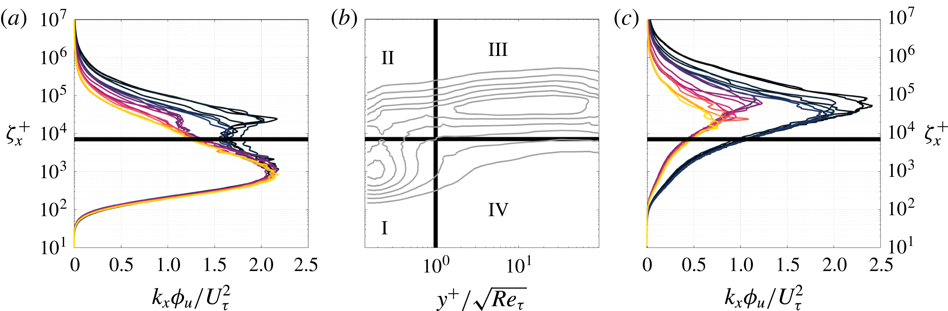
From here, one can construct a conceptual model that appears to govern the spectral scaling for a TBL subjected to FST. For this model, the spectrogram is divided into four regions separated along $y^{+}=\sqrt{Re_{\unicode[STIX]{x1D70F}}}$ and $\unicode[STIX]{x1D701}_{x}^{+}=7000$ . The divider in wavelength separates the large and small scales as discussed in the previous section. These regions are depicted in figure 11(b) and can be described as follows.

1. (I) ( $y^{+}<\sqrt{Re_{\unicode[STIX]{x1D70F}}},\unicode[STIX]{x1D701}_{x}^{+}<7000$ ): This region is home to the near-wall spectral peak (typically centred at $y^{+}\approx 15$ , $\unicode[STIX]{x1D701}^{+}\approx 1000$ ). The near-wall spectral peak scales with viscous units, making its location, shape and normalised magnitude universal when normalised. This means that we can use this information to obtain skin friction of boundary layers under the influence of FST. For example, a hot-wire measurement in the near-wall region could be used in liaison with the scaling identified here to determine $U_{\unicode[STIX]{x1D70F}}$ and hence $C_{f}$ by adjusting the estimate of $U_{\unicode[STIX]{x1D70F}}$ until the inner peak was collapsed on the expected value.

2. (II) ( $y^{+}<\sqrt{Re_{\unicode[STIX]{x1D70F}}},\unicode[STIX]{x1D701}_{x}^{+}>7000$ ): This region is influenced by variations in the FST. Increases in $u_{\infty }^{\prime }/U_{\infty }$ penetrate all the way to the wall, resulting in an increase in $U_{\unicode[STIX]{x1D70F}}$ and correspondingly $Re_{\unicode[STIX]{x1D70F}}$ . This occurs because the energy that exists at the large wavelengths is not transferred to the near-wall peak in region (I) such that the latter is fixed and universal. Note that because the near-wall peak in region (I) is collapsed for all tested $u_{\infty }^{\prime }/U_{\infty }$ and $Re_{\unicode[STIX]{x1D70F}}$ , it suggests that the increase in area under the spectral curve at $\unicode[STIX]{x1D701}_{x}^{+}>7000$ is proportional to the growth in $U_{\unicode[STIX]{x1D70F}}$ . Changes in $L_{u,\infty }$ penetrate down to this region (figure 5), but do not appear to influence the mean velocity or variance profiles for the $u_{\infty }^{\prime }/U_{\infty }$ investigated here.

3. (III) ( $y^{+}>\sqrt{Re_{\unicode[STIX]{x1D70F}}},\unicode[STIX]{x1D701}_{x}^{+}>7000$ ): In this region, the boundary layer acts as a universal filter to the most energetic wavelengths in the free-stream spectrum. It preferentially amplifies certain wavelengths, resulting in the outer peak. The amplification is independent of $u_{\infty }^{\prime }/U_{\infty }$ , and hence this region is governed by global laws different from those in region (I).

4. (IV) ( $y^{+}>\sqrt{Re_{\unicode[STIX]{x1D70F}}},\unicode[STIX]{x1D701}_{x}^{+}<7000$ ): This region is not home to a significant amount of the energy and seemingly does not play as strong a role in the dynamics.

Figure 11.

(a) Inner-normalised pre-multiplied spectra at $y^{+}\approx 15$ for all cases. (b) Conceptual map identifying four regions in a generic spectrogram of a TBL subjected to FST. (c) Inner-normalised pre-multiplied spectra in the free stream for all cases. For the spectra, the lightest to darkest lines represent increasing $u_{\infty }^{\prime }/U_{\infty }$ . The identified regions are separated along $y^{+}/\sqrt{Re_{\unicode[STIX]{x1D70F}}}=1$ and $\unicode[STIX]{x1D701}^{+}=7000$ .

This model explains the increase in $U_{\unicode[STIX]{x1D70F}}$ with increasing $u_{\infty }^{\prime }/U_{\infty }$ and suggests that a measurement at $y^{+}\approx 15$ is sufficient to estimate $U_{\unicode[STIX]{x1D70F}}$ for these flows. Furthermore, one can in principle predict the location of both the inner and outer spectral peaks given the spectrum of the FST. This is because $G_{g}$ approximately describes the flow in regions (II), (III) and (IV), and region (I) is independent of the other regions. We thus propose using $G_{g}$ to reconstruct the flow in regions (II), (III) and (IV) from only the free-stream spectrum, and then using the inner peak from our best-resolved case (A) in region (I) to reconstruct the same cases as shown in figure 10. Ideally, the inner peak geometry would come from an analytical expression; however, for the time being our best-resolved measurement of the empirical curve will suffice. This proposed reconstruction process is illustrated in figure 12, where weighting functions are used to blend the inner peak reconstruction (region (I)) with the gain reconstruction (regions (II)–(IV)). The weighting decays linearly outside of the bounds specified in the conceptual model to a total extent of five times the limit. The results of this reconstruction are presented in figure 13, where it can be seen that both the inner and outer peaks are now captured by the reconstruction methodology based on only the free-stream spectrum; both the location and magnitude of the inner peak are now in agreement between the reconstruction and the measured spectrograms to within 6 %, a vast improvement over figure 10 where only the gain function was used.

Figure 12.

Proposed reconstruction methodology. Region (I) in figure 11 is constructed from the inner peak of a well-resolved case. Regions (II), (III) and (IV) are constructed by multiplying the free-stream spectrum by the global gain function ( $G_{g}$ ) and a weighting function. These two spectrograms are then summed to produce the reconstruction.

Figure 13.

Reconstructed spectrograms using the methodology presented in figure 12 for (a) case C, (b) case G and (c) case N from table 1. The corresponding difference maps between the reconstructed and measured spectrograms are given in (d), (e) and (f), respectively, as $\unicode[STIX]{x1D6E5}_{C}=(\unicode[STIX]{x1D719}^{+}-\tilde{\unicode[STIX]{x1D719}}^{+})/\unicode[STIX]{x1D719}^{+}$ . The solid lines represent contours at $\unicode[STIX]{x1D719}^{+}=0.9$ , 1.2, 1.5, 1.8 and 2.1 from the measured spectrograms. The solid line contours increase from outermost to innermost. The vertical dashed lines are at $y^{+}=\sqrt{Re_{\unicode[STIX]{x1D70F}}}$ .