

I. Introduction
When borrowing needs change quickly, bills are our issuance ‘shock absorber.’ Because we want nominal coupon securities to adjust gradually, bills play an important role in managing changes in borrowing needs that are […] unexpected. (Scott Bessent, Secretary of the U.S. Treasury, Nov. 12, 2025)
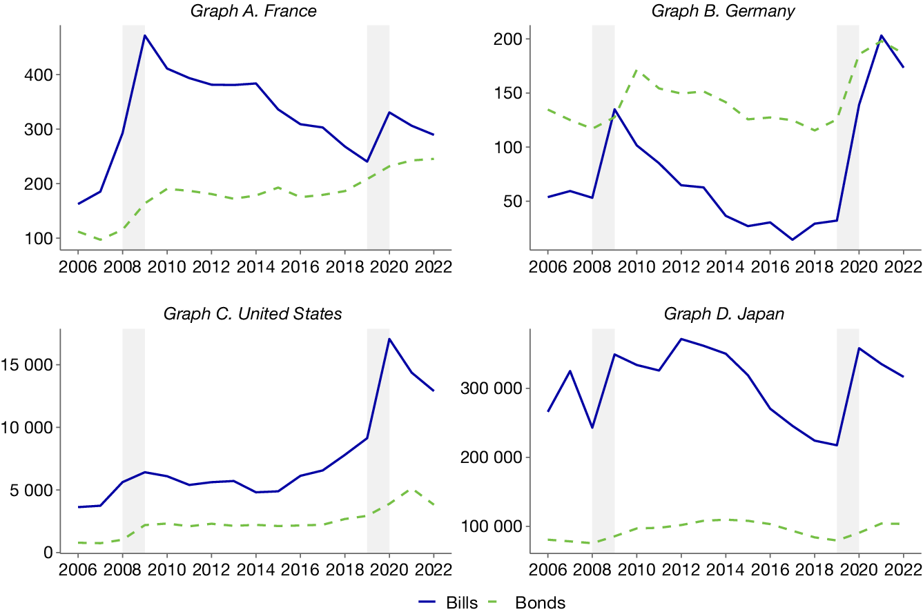
Governments across the world perceive it is easier to issue additional short-term debt (bills) unexpectedly than long-term debt (bonds or “coupon securities”). This can be read in the preceding quote and in similar statements made in various countries as well as by international institutions.Footnote 1 This feature of modern debt management appears clearly in the data during crises, when deficits rise sharply. For example, during the great recession (2008–2009) or the pandemic (2020–2021), many countries had to immediately issue significant amounts of public debt to finance large deficits. They decided to do so overwhelmingly through the use of Treasury bills, that is, debt securities with an initial maturity of 1 year or less. This can be seen in Figure 1, which shows the issuance breakdown between bills and bonds of 4 countries with completely different fiscal frameworks and traditions: France, Germany, the United States, and Japan.
Figure 1 shows the nominal amount of bills (solid blue line) and bonds (dashed green line) issued per year and per country. Shaded areas indicate crisis years. Section A of the Supplementary Material shows outstanding amounts. Bills are defined as debt securities with 1 year of initial maturity or less. We classify all other debt securities as bonds. We group notes and bonds together for the United States as this distinction does not exist in most countries. Source: National Ministries of Finance’s websites.

FIGURE 1 Long description
The multi-panel figure consists of four line graphs arranged in a two-by-two grid. Each graph shares a common X-axis representing years from 2006 to 2022 and includes two vertical shaded gray bars indicating crisis periods around 2008 to 2009 and 2019 to 2020. A legend at the bottom indicates that solid blue lines represent Bills and dashed green lines represent Bonds.
* Top-Left Panel (France): The Y-axis ranges from 100 to 400. Bills show a sharp peak near 450 in 2009, followed by a gradual decline and a secondary peak in 2020. Bonds remain lower, showing a steady upward trend from 100 in 2006 to approximately 250 in 2022.
* Top-Right Panel (Germany): The Y-axis ranges from 50 to 200. Bonds generally stay above bills until 2021. Bills spike during both crisis periods, reaching their highest point of 200 in 2021. Bonds fluctuate between 120 and 175, ending near 175.
* Bottom-Left Panel (United States): The Y-axis ranges from 0 to 15,000. Bills significantly outweigh bonds. Bills show a moderate increase in 2009 and a massive surge to over 15,000 in 2020. Bonds remain relatively flat below 5,000 throughout the period.
* Bottom-Right Panel (Japan): The Y-axis ranges from 100,000 to 300,000. Bills show high volatility, with major peaks in 2009, 2012, and 2020, staying consistently above 200,000. Bonds remain stable and much lower, fluctuating slightly around the 100,000 mark.
In most countries, when deficits increase, this translates into a permanent jump in the debt stock. This is because usually no systematic fiscal measures are voted to offset these negative shocks. The decline of GDP over 1 year is a permanent loss which may be partially recovered subsequently but will leave public finance strained for several years. There is a priori no reason to finance a permanent increase in debt with short-term securities, which are usually seen as carrying higher refinancing and interest rate risk for sovereign issuers. The relative price of issuing at short versus long maturities (the term premium) did not appear to change in favor of the former type of debt during the episodes discussed previously (e.g., Berardi (Reference Berardi2023)). Moreover, we could not find any legislation limiting the recourse to long-term debt in recent years.Footnote 2
In this article, we show empirically that indeed bond yields increase by more than bill yields in case of a surprise issuance, that is, in the short run, governments face a steeper demand curve on the bond market than on the bill market. This feature applies in normal times and in crisis times. To be sure, we will show that when governments want to sell debt, the prices (resp. yields) of bills fall (resp. rise) by less than the price (resp. yield) of bonds. By conservative estimates, bond yields increase by around four times more than bill yields after auction announcements and before actual issuance, costing the Treasury as much. Moreover, the increase in the yield is partially reversed for bills after auctions but is persistent for bonds. These additional costs lead debt management offices (DMOs) to use bills as their first line of defense to accommodate large and permanent shocks. They substitute slowly toward bond issuance thereafter (see opening citation and Figure 1). As we will show, bond market investors need to be prepared in advance to absorb additional issuance, and may be able to do so but over longer periods of time.
We use the case of France as its institutional setting offers many advantages. First, it is the largest issuer of euro-denominated Treasury bills. We present evidence that French T-bills were considered safe assets during our sample period. Second, most issuances are “reopenings” or “re-issuance.” That is, to borrow funds, the French Treasury usually sells more or “increases the size” of an existing security that was already created and tendered years before. This allows us to look at the effect of issuing a given security on the secondary market yield of that same security several days before and after the issuance. Secondary market yields are a good proxy for financing cost. As we show, they are on average equal to primary market yields on auction day and are available before and after the auction. Third, the reopenings are not fully expected by the market, allowing us to assess the effects of unexpected issuance of bills and bonds.Footnote 3 Fourth, the French Treasury established a similar procedure for issuing bills and bonds, but auctions occur on different days of the week, making it easy to compare the price impact of each type of securities issuance.
Auction routine has remained virtually unchanged for the last 40 years in France, contrary to other countries such as the United States (Garbade (Reference Garbade2015)). During this period, reopenings occur once to twice per week, providing us with plenty of observations. Auctions and announcements always take place on the same days of the week (public holidays excepted). The securities to be issued are not known to the market prior to announcements, triggering supply shocks in a given securities’ market, which we exploit.
Methodologically, we use a lead–lag model to estimate the impact of the issuance of a given French Treasury security on its end-of-day secondary market yield, 1 week before and 1 week after the auction. Our specifications are close to Lou, Yan, and Zhang (Reference Lou, Yan and Zhang2013), who look at the impact of new (“on-the-run”) bond issuance on the secondary market yield of previously issued (“off-the-run”) bonds in the United States. We augment these regressions with date fixed effects, security fixed effects, and additional control variables. We also consider bills (not only bonds) and look at the impact of a given securities issuance on its own secondary market yield, which is possible thanks to the practice of re-issuance.
We show that announcements of re-issuance cause an immediate market reaction, ahead of the auction itself. Our regressions indicate that between announcement and issuance a bond typically sees its yield increase by up to 2.8 basis points per billion issued, while over the same period, a bill sees its yield increase by 0.9 basis points. Other regressions find more modest effects but put the difference between bills’ and bonds’ reactions at 1 to 4. We also run our regressions in percentage of GDP, as opposed to per billion issued and in proportion of each security’s outstanding amount. The difference in price impact remains between 1 to 3 and 1 to 4. The difference rises to 1 to 5 in our robustness exercises. Our empirical setup is able to identify yield changes over a few days only, but they matter for public finance because we show that yields peak exactly on the day of issuance. In other words, even if these yield increases were to be short-lived, the Treasury bears their full cost. These estimates are in line with those found in other countries for the response of bond yields (the response of bills being largely unexplored).
Our identification strategy relies on (supply) surprises regarding the security that will be re-issued and how much of it will be re-issued. This strategy is valid if the market cannot better anticipate which bill will be re-issued than which bond will be re-issued, and how much of it will be re-issued. If anything, there is greater variability in issuance for bills and correspondingly higher ex ante uncertainty. This greater variability can be seen, for instance, in Figure 1, in Section A of the Supplementary Material, and in our descriptive statistics, which will show that the standard deviation of bill issuances is larger than bond issuances. Moreover, we will show that there are an equivalent number of bills and bonds that can be re-issued at any point in time, and in fact slightly fewer bonds than bills, suggesting again that any surprise effects should be larger for bills. Thus, there is no reason to believe that issuances can be better anticipated for bills than for bonds, but rather the opposite.
We account for the possibility of reverse causality in case the Treasury strategically issues more debt when yields increase only modestly after the announcement of an issuance. Such strategic behavior from the DMO would bias our price impact estimates toward 0. For that purpose, we use announced amounts as opposed to amounts actually issued. We control for demand, following the same method as Ray, Droste, and Gorodnichenko (Reference Ray, Droste and Gorodnichenko2024) and Kacperczyk, Pérignon, and Vuillemey (Reference Kacperczyk, Pérignon and Vuillemey2021). Moreover, we explicitly account for the large bond purchases of the ECB and euro area national central banks under its various Quantitative Easing (QE) programs, a key event during our sample period. We also control for periods of crises, such as the great recession and the pandemic, to demonstrate that our results are not driven by the demand for short-term safe assets in times of stress.
We next turn our attention to the channels through which bond issuances increase yields by more than bill issuances. One natural candidate to explain this phenomenon is duration risk: as the Treasury injects duration risk in the market, the price of high-duration assets (bonds) should fall (i.e., yields should rise), in a symmetric fashion from QE (Krishnamurthy and Vissing-Jorgensen (Reference Krishnamurthy and Vissing-Jorgensen2012), Greenwood and Vayanos (Reference Greenwood and Vayanos2014)). However, we show that duration risk is not a major driver in our results. We split our bond sample into three: “short-,” “medium-,” and “long”-term bonds. Bonds most affected by additional issuance are, in fact, those with the shortest maturity.
We also run regressions using the spread between yields and overnight index swap (OIS) rates as our dependent variable. This measure should be purged of the expected path of short-term interest rates and of the term premium of euro-denominated assets. The impact of additional issuance on this spread should be 0 if yields move due to an increase in the term premium. In fact, we show that this variable reacts almost exactly like bond yields to issuance, suggesting that auctions depress asset prices but are not large enough to affect the term premium in euro. This analysis is possible because we study one of many countries of the euro area, and the OIS market in euro is larger than its sovereign bond market (Dalla Fontana, Holz auf der Heide, Pelizzon, and Scheicher (Reference Dalla Fontana, Holz auf der Heide, Pelizzon and Scheicher2019)). Moreover, interest rate swaps are cleared and thus collateralized, purging them of any credit risks. OIS rates are routinely used for high-frequency identification of monetary policy shocks, demonstrating their capacity to react at least as quickly as bond yields.
These results are most consistent with the theory of “preferred habitat” as modeled by Vayanos and Vila (Reference Vayanos and Vila2021). In that setting, the different demand curves of preferred habitat investors for each specific maturity play a key role in explaining how yields react to demand shocks. In the presence of preferred habitat investors alongside arbitrageurs with limited risk-bearing capacity, the price impact is not monotonously increasing in the duration of the security.
In the presence of preferred habitat and risk-averse arbitrageurs, additional supply at one maturity point propagates to yields of bonds with close maturities, as noted by Ray et al. (Reference Ray, Droste and Gorodnichenko2024) and Selgrad (Reference Selgrad2023). We extend this reasoning to supply shocks, such as additional issuance of specific securities by the Treasury. We show that indeed the price impact of the supply of bonds propagates to securities of similar maturities, while the supply of bills does not. The effect decays as the distance between two bonds along the yield curve grows. This pattern is consistent with bond investors having stronger preferences for specific maturities compared to bill investors.
With these results at hand, we go on and explore why investors in the bill market have flatter demand curves than in the bond market, at least in the short run. We show that standard metrics of secondary market liquidity do not explain this feature of T-bills. To be sure, contrary to the literature’s consensus, bills are in general less liquid than bonds on the secondary market. Indeed, we find that in France the bid–ask spread for bills is around five times as large as for bonds. Thus, we conclude that the ease to sell bills on the primary market is not explained by liquidity in the secondary market.
We present evidence that investors in the T-bill market are large-pocketed foreign institutions looking for safety. They buy and hold T-bills to maturity, thus rendering bills relatively illiquid. Investors in the bond market are, by and large, pension funds and insurance companies comfortable with taking duration risk but with little flexibility in the amounts they invest in the short run. Thus, they are unable to immediately accommodate higher supply from the Treasury in the category of assets they hold (bonds). As time goes on and they receive more cash from their customers, they may be able to absorb additional supply of bonds.
The main contribution of this article is to improve our understanding of preferred habitat. Using debt supply shocks, we are able to study the demand curve not only for bonds but also for bills. This could not be done in the QE literature because bills are typically not part of central bank asset purchase programs. We also show that some agents (insurance companies, pension funds, and foreigners) have preference for specific points of the yield curve but that this is not only due to the amount of duration risk that a given security carries, especially for bonds. Moreover, we provide evidence of significant costs, by the literature’s standards, of surprise issuance of one type of security over the other. As shown by Faraglia, Marcet, Oikonomou, and Scott (Reference Faraglia, Marcet, Oikonomou and Scott2019), the issuance costs associated with auction announcements have dramatic implications for debt maturity and theoretically rationalize the use of short-term debt by sovereign issuers.Footnote 4 Our findings thus contribute to the understanding of governments’ reliance on Treasury bills when they need to raise money quickly. Incidentally, our findings are also useful to estimate the effect of a potential Quantitative Tightening (QT) program, under which central banks announce the sale of some of their securities holdings.
The rest of this article is organized as follows: Section II reviews the literature, and Section III describes the institutional background. Section IV details our empirical strategy and results. Section V presents evidence on the ownership structure of bills and bonds. Section VI concludes.
II. Literature Review
Our article first contributes to the fast-expanding literature on preferred habitats, as theoretically modeled by Vayanos and Vila (Reference Vayanos and Vila2021). Empirically, some studies (e.g., Greenwood and Vayanos (Reference Greenwood and Vayanos2014) or more recently Gomez Cram, Kung, and Lustig (Reference Gomez Cram, Kung and Lustig2025)) insist on the price of duration risk along the whole curve to explain yield variations following debt supply shocks. Other studies such as Ray et al. (Reference Ray, Droste and Gorodnichenko2024), Selgrad (Reference Selgrad2023), or Lucca and Wright (Reference Lucca and Wright2024) stress the “local” effects of supply and demand shocks on the yield curve, a pattern most consistent with the presence of preferred habitat investors. Using the institutional setup of France, with frequent re-issuance and a large OIS market, we are able to show that duration risks play a minor role in explaining yield changes around debt issuance. Lastly, we document that governments lean primarily on the T-bill debt market in case of shocks to the budget and extend the maturity of their liabilities afterward. This suggests that bond investors can be relatively price-inelastic with strict quantity targets in the short run, but that their demand may grow in the medium run, suggesting a dynamic dimension to preferred habitat.
Our article has implications for the literature on the optimal maturity of debt. Seminal contributions in this field include inter alia Lucas and Stokey (Reference Lucas and Stokey1983), Angeletos (Reference Angeletos2002), and Aiyagari, Marcet, Sargent, and Seppala (Reference Aiyagari, Marcet, Sargent and Seppala2002). These articles model a Ramsey planner issuing risk-free debt. The main conclusion is that governments should issue large amounts of long-term debt and hold short-term assets (i.e., negative issuance of short-term debt). Moreover, the government should buy back the whole stock of long-term debt and issue new long-term debt every year. As shown by Buera and Nicolini (Reference Buera and Nicolini2004), this leveraged strategy would imply borrowing amounts equivalent to multiples of GDP in the long-term debt market. Such debt management recommendations are far remote from the observed behavior of governments. In order to bring theory closer to the practice of DMOs, Faraglia et al. (Reference Faraglia, Marcet, Oikonomou and Scott2019) introduced transaction costs of issuing debt in a theoretical model. Once these costs are accounted for, theory delivers a more realistic maturity profile and gives a role to short-term debt issuance Faraglia et al. (Reference Faraglia, Marcet, Oikonomou and Scott2019). To the best of our knowledge, our article is the first one to show that issuance costs are lower for bills than for bonds and that it is therefore less costly to issue such short-term debt when resources are needed quickly.
We also contribute to the literature on the price impact of sovereign debt auctions. Although sovereign debt issuance in OECD countries is typically regular and predictable events, they have an impact on securities prices when they occur. This has been shown in the case of the United States (Lou et al. (Reference Lou, Yan and Zhang2013), Phillot (Reference Phillot2025), and Ray et al. (Reference Ray, Droste and Gorodnichenko2024)), Canada (Allen, Hortacsu, Richert, and Wittwer (Reference Allen, Hortacsu, Richert and Wittwer2024)), the United Kingdom (Lengyel (Reference Lengyel2022)), Spain (Bigio, Nuno, and Passadore (Reference Bigio, Nuno and Passadore2023)), Portugal (Albuquerque, Cardoso-Costa, and Faias (Reference Albuquerque, Cardoso-Costa and Faias2024)), Germany (Beetsma, Giuliodori, de Jong, and Widijanto (Reference Beetsma, Giuliodori, de Jong and Widijanto2016)), Italy (Sigaux (Reference Sigaux2024)), and Switzerland (Cavaleri, Ranaldo, and Rossi (Reference Cavaleri, Ranaldo and Rossi2025)). Arcidiacono, Bellon, and Gnewuch (Reference Arcidiacono, Bellon and Gnewuch2024) show that the issuance of German benchmark bonds reduces the convenience yield of their French counterpart, nearly one-for-one.Footnote 5 To our knowledge, no study has ever shown the lower impact of bill auctions, and therefore their advantage over bonds to finance quickly extra funding needs.Footnote 6 Given that France is the largest euro-area issuer of T-bills, it provides an ideal laboratory to study this question.
Lastly, our article sheds new light on the nature of safe assets. While many contributions have explored the properties of safe assets from the demand side in periods of crises (Greenwood, Hanson, and Stein (Reference Greenwood, Hanson and Stein2015), Gorton and Ordonez (Reference Gorton and Ordonez2022)), we show that T-bills face a relatively flat demand curve at all times. This may trigger their volume to rise during crisis also due to higher supply and not just increased demand. While often assumed in the literature, we also show that safe assets such as bills are not clearly more liquid than bonds by conventional metrics.
III. Institutional Background
DMOs in high-income countries nowadays issue securities in a “regular and predictable manner.” This approach was developed in the United States by Paul Volcker when he was a Treasury official in the 1970s (Garbade (Reference Garbade2015)). It is believed that minimizing surprises, as opposed to “opportunistic” issuances, leads to lower volatility in the government securities market, which improves the safety characteristics of Treasury securities and in turn leads to lower funding costs over the medium run (Garbade (Reference Garbade2007)), as summarized by then-assistant Treasury secretary Powell before the U.S. Congress:
“Treasury believes that the best way to achieve the goal of minimizing borrowing costs to the U.S. taxpayer is to minimize surprises to the market.” Jerome Powell (1991)
This feature of modern debt management implies that any effect we observe on the yield of a security around auction is by construction extremely small, as the DMO intends to minimize volatility by implementing such a regular and predictable routine.
The French DMO, the Agence France Trésor (AFT), issues T-bills (Bon du Trésor à taux Fixe or BTF) on Monday every week. Typically, three different bills may be issued (e.g., with 3-month, 6-month, and 12-month residual maturity).
On the first Thursday of the month, the French DMO issues long-term bonds, “Obligation assimilable du Trésor” (OAT) with 7-year residual maturity or more. Three different bonds are typically issued on those days (e.g., 8, 10, and 12-year). On the third Thursday of the month, medium-term bonds between 2- and 8-year maturity are issued. These medium-term bonds are also issued in batches of 3 (e.g., 3, 5, and 6-year).
This regular and predictable auction process was introduced in 1986 in the context of a large-scale financial markets reform in France (Pons (Reference Pons1988)) and has been little changed since. We begin our study in January 1999, the start of the single currency, and thus avoid dealing with franc-denominated securities.
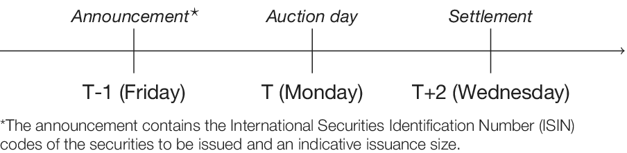
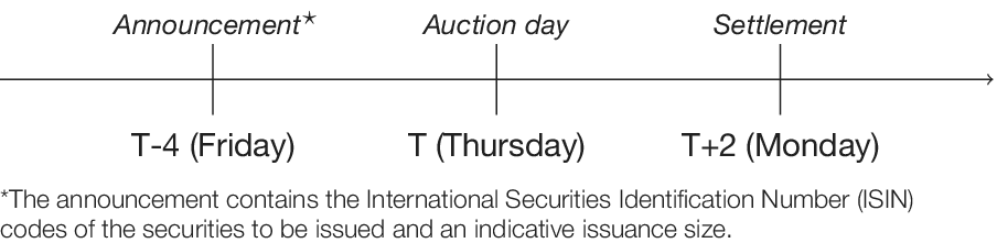
Every Friday, the Treasury announces which securities (identified by codes and maturity dates) will be (re)-issued on Monday and Thursday of the following week. That is, announcements come on T–1 and T–4 for bills and bonds, respectively (see Figures 2 and 3). Indicative volumes are also communicated. Crucially, exactly which security (bills or bonds) will be issued during the following week is not known before the announcement, except for “benchmark” bonds. Historically, announcements came at various times during the day, and we were not immediately able to identify these moments. For that reason, we feel more comfortable using daily end-of-day secondary market yields than intraday data.
Figure 2 represents the timeline of issuance for French Treasury bills.

Figure 3 represents the timeline of issuance for French Treasury bonds.

On auction day (every Monday and two Thursdays per month), bids are submitted and ranked in ascending order for each security (bids carrying the lowest yields receiving priority). The exact size of the issuance, within the pre-announced range, remains at the discretion of the Treasury. This is different from the U.S. setup where the exact dollar amount to be issued is known in advance (Ray et al. (Reference Ray, Droste and Gorodnichenko2024)). If selected, participants pay the price they bid for (multiple price auction). Only primary dealers (around 15 banks) can bid, unlike in the United States (Amin and Tédongap (Reference Amin and Tédongap2023)).
In December of each year, the French Treasury announces the total amount of bonds it intends to issue the following year. The Treasury also announces which “benchmark” bonds it will issue. These are typically one new 3-year bond, a new 5-year bond, and one or two 10-year bonds. These bonds are, however, never issued in one go, but most often in six consecutive times. During these six auctions, the new benchmark bond is said to be “on-the-run,” meaning it is the newest bond of this maturity bucket to have been created. When a newer bond of the same maturity bucket comes into existence, the previous bond becomes “off-the-run.”
Another important difference with the United States is that off-the-run bonds are a significant part of the financing of the French Treasury. They represented around half of the financing in our sample. It is not rare to see a 10-year bond being re-issued eight times while off-the-run. A couple of 10-year were re-issued up to 11 times in our sample while off-the-run. Issuance of off-the-run bonds is more frequent on average than on-the-run bonds.
The amount of T-bills to be issued is not announced in December of each year, nor which tenor will be issued. This difference with the well-prepared schedule for bonds already suggests that, in the short run, bond investors are less equipped to absorb large quantities of additional securities.
IV. Empirical Strategy
A. Data
We gather data on the issuance of sovereign bills and bonds from the website of the French DMO (AFT) from January 1999 to December 2022, including auction dates, amounts issued of each security (identified via the International Securities Identification Number, ISIN), pre-announced range of the issuance for each ISIN (available only for bills), and maturity date of the security. We merge our ISIN-issuance data set with end-of-day secondary market yield-to-maturity from Bloomberg. Our daily panel of securities goes from January 1999 to December 2022. We also collect OIS rates, available in Bloomberg from 2004.
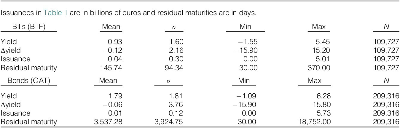
We remove outliers in terms of one-day change of yield-to-maturity (our main variable of interest) by taking out the 0.5% of the distribution on both sides, that is, we ignore 1% of observations. We remove inflation-linked and green bonds. Lastly, we remove the last 30 days of the life of each Treasury security as their yields display much larger volatility right before being redeemed, and no security is re-issued so close to maturity. Tables 1 and 2 display descriptive statistics for each type of security in the sample after these cleanings are implemented, for all days (Table 1) during the sample period and on auction days only (Table 2).

TABLE 1 Long description
The table is divided into two sections.
Section 1: Bills B T F.
Columns are Mean, sigma, Min, Max, and N.
Row 1: Yield. Mean 0.93, sigma 1.60, Min minus 1.55, Max 5.45, N 109,727.
Row 2: Delta yield. Mean minus 0.12, sigma 2.16, Min minus 15.90, Max 15.20, N 109,727.
Row 3: Issuance. Mean 0.04, sigma 0.30, Min 0.00, Max 5.01, N 109,727.
Row 4: Residual maturity. Mean 145.74, sigma 94.34, Min 30.00, Max 370.00, N 109,727.
Section 2: Bonds O A T.
Columns are Mean, sigma, Min, Max, and N.
Row 1: Yield. Mean 1.79, sigma 1.81, Min minus 1.09, Max 6.28, N 209,316.
Row 2: Delta yield. Mean minus 0.06, sigma 3.76, Min minus 15.90, Max 15.80, N 209,316.
Row 3: Issuance. Mean 0.01, sigma 0.12, Min 0.00, Max 5.73, N 209,316.
Row 4: Residual maturity. Mean 3,537.28, sigma 3,924.75, Min 30.00, Max 18,752.00, N 209,316.

TABLE 2 Long description
The table is divided into two sections.
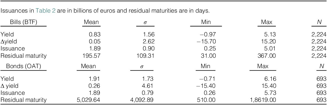
Section 1: Bills B T F. Columns include Mean, sigma, Min, Max, and N.
* Yield: Mean 0.83, sigma 1.56, Min minus 0.97, Max 5.13, N 2,224.
* Delta yield: Mean 0.05, sigma 2.62, Min minus 15.70, Max 15.20, N 2,224.
* Issuance: Mean 1.89, sigma 0.90, Min 0.25, Max 5.01, N 2,224.
* Residual maturity: Mean 195.57, sigma 109.31, Min 31.00, Max 367.00, N 2,224.
Section 2: Bonds O A T. Columns include Mean, sigma, Min, Max, and N.
* Yield: Mean 1.91, sigma 1.73, Min minus 0.71, Max 6.16, N 693.
* Delta yield: Mean 0.26, sigma 4.61, Min minus 15.40, Max 15.40, N 693.
* Issuance: Mean 1.89, sigma 0.79, Min 0.26, Max 5.73, N 693.
* Residual maturity: Mean 5029.64, sigma 4092.89, Min 510.00, Max 18619.00, N 693.
Naturally, the yield level (measured in percentage points) is on average larger for bonds than for bills, just like the standard deviation. This is consistent with a positive term premium on average and the larger duration risk associated with bonds compared to bills. The yield change (measured in basis points), which will be our main variable of interest, is centered around 0 and is nearly perfectly symmetric, as shown by the minimum and the maximum values. Once again, the standard deviation is understandably larger for bonds than for bills. Interestingly, the average issuance size, as shown in Table 2, is equal for bonds and bills during our sample period. The standard deviation of issuance is larger for bills, consistent with our stylized facts, suggesting a capacity for the Treasury to vary the issuance size for T-bills to a greater extent than for bonds.
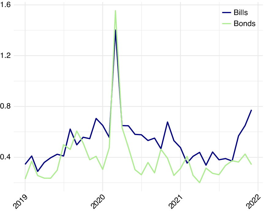
Suggestive evidence of the ability of the Treasury to vary T-bill issuance can also be seen in auction prices. More specifically, one can look at the difference between the marginal rate of the auction (i.e., the least competitive accepted bid) and the average yield of accepted bids. This difference should represent the steepness of the demand curve for each bill and bond for the quantities supplied by the Treasury at each auction. This spread can be seen in Figure 4. One can see that while the difference is always below 1 basis point, it increased markedly during COVID-19, and more so for bonds than for bills, even though the supply of the latter was raised significantly more than that of the former. Unfortunately, marginal rates data are only available from 2019. Moreover, as explained in the next subsection, marginal and average rates are by definition only available on auction days, which is why we rather use secondary market yields for our empirical analysis.
Figure 4 shows the spreads between the marginal rate and the average rate at auctions for both bills and bonds between 2019 and 2022. Source: French debt management office’s website.

FIGURE 4 Long description
The X axis represents time from 2019 to 2022. The Y axis represents basis points ranging from 0.0 to 1.6 in increments of 0.4. Two lines are plotted: a dark blue line for Bills and a light green line for Bonds.
* From 2019 to early 2020, both series fluctuate between 0.2 and 0.6 basis points.
* In early 2020, both lines experience a sharp, near-vertical spike. The Bonds line peaks at approximately 1.55 basis points, while the Bills line peaks slightly lower at approximately 1.4 basis points.
* Following the peak, both series drop sharply. Throughout late 2020 and 2021, the Bills series generally remains higher than the Bonds series, fluctuating between 0.4 and 0.7 basis points.
* The Bonds series remains lower, mostly between 0.2 and 0.4 basis points, reaching its lowest point in early 2021.
* By the end of 2021, the Bills series shows a sharp upward trend toward 0.8 basis points, while the Bonds series remains relatively flat near 0.35 basis points.
B. Specifications
Our goal is to estimate the effect of government debt issuance on yield-to-maturity, which is ultimately what matters most to an issuer. Secondary market yields can serve as a proxy for primary market rates, which are by definition only available on auction days. Looking at the secondary market yield therefore allows to exploit more time series (several days before and after issuance) and cross-sectional variations (all outstanding ISINs at one point in time and not only those re-issued). We check that in our sample the primary and secondary market yields are similar on auction days. As shown in Figure 2 in the Supplementary Material, this is indeed the case. The difference between primary and secondary market yield is on average 0 and uncorrelated with the amount issued.
Since we want to look at secondary market yields a few days before issuance, we cannot include newly issued bonds in our sample. Moreover, the so-called “benchmarks” are around three new bonds of standard maturity issued each year. These maturities are 3-, 5-, and 10-year. These bonds are issued around six times in a row. During those months, the market knows that these bonds will be issued for sure. It makes these bonds hardly comparable with other securities, which re-issuance is uncertain. For that reason, we exclude these benchmarks when they are “on-the-run,” that is as long as a newer benchmark has not been issued.
We run the following lead–lag model, separately for bills and bonds, to take into account announcement effects as well as post-issuance dynamics for each type of securities:

where
$ \Delta {Y}_{i,t} $
 is the daily change in the mid-secondary market yield-to-maturity of ISIN
$ i $
 (expressed in basis points) between
$ t-1 $
 and
$ t $
 .
$ {X}_{i,t+n} $
 is the nominal amount of security i issued (variation of the total amount outstanding) on day
$ t+n $
 , where t is the date and n is an integer from −5 to 5 representing business days before and after issuance.Footnote
7 After looking at our results for 1 billion euro issued, we replace
$ {X}_{i,t+n} $
 by other indicators of issuance, such as dummy variables equal to 1 when there is an auction, and 0 otherwise. We also use announced amounts for that security’s auctions instead of amounts actually issued.
We include both ISIN fixed effects (
$ {f}_i $
 ) as well as date fixed effects (
$ {f}_t $
 ), to control notably for high-frequency shifts in demand (Kacperczyk et al. (Reference Kacperczyk, Pérignon and Vuillemey2021)).
C. Baseline Results
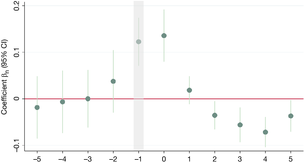
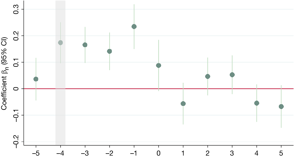
The coefficients of our regressions are displayed in Figure 5 for bills and Figure 6 for bonds. We observe a positive and significant reaction at the 1% level prior to the auction day (represented by day 0). Bills react 1 business day before the auction date, while bonds react already 4 business days prior.
Figure 5 plots the yield change (in basis points) on days prior to and after the issuance of a specific security. Auction day is day 0. The shaded areas mark announcement day (T–1 for bills and T–4 for bonds). Issuance is defined here as 1 billion euro issued. Yield changes are not cumulative from one day to the next.

FIGURE 5 Long description
The Y-axis is labeled Coefficient beta sub n open parenthesis 95 percent C I close parenthesis, ranging from negative 0.1 to 0.2. A horizontal red line marks the zero baseline. The X-axis represents days relative to the auction, ranging from negative 5 to 5.
Data points are represented by green circles with vertical error bars indicating the 95 percent confidence interval.
* From day negative 5 to negative 3, the coefficients are near zero or slightly negative.
* At day negative 2, the coefficient rises to approximately 0.04.
* Day negative 1 is highlighted with a vertical gray shaded area, showing a sharp increase to approximately 0.12.
* Day 0, the auction day, shows the peak coefficient at approximately 0.14.
* Following the auction, the values drop sharply. Day 1 is near 0.02, and days 2 through 5 fall below the zero baseline, reaching a low of approximately negative 0.07 at day 4.
Figure 6 plots the yield change (in basis points) on days prior and after the issuance of a specific security. Auction day is day 0. The shaded areas mark announcement day (T–1 forbills and T–4 for bonds). Issuance is defined here as 1 billion euro issued. Yield changes arenot cumulative from one day to the next.

FIGURE 6 Long description
A line graph with a horizontal x-axis ranging from minus 5 to 5 and a vertical y-axis labeled Coefficient beta sub n 95 percent C I ranging from minus 0.2 to 0.3. A solid red horizontal line marks the zero baseline.
Data points are represented by dark green circles with vertical error bars.
- At x equals minus 5, the point is slightly above 0.
- At x equals minus 4, which is highlighted by a vertical light gray shaded band, the point rises to approximately 0.18.
- At x equals minus 3, the point is around 0.17.
- At x equals minus 2, the point is around 0.14.
- At x equals minus 1, the point reaches its peak at approximately 0.24.
- At x equals 0, the point drops to approximately 0.09.
- At x equals 1, the point falls below the zero line to approximately minus 0.06.
- At x equals 2 and 3, the points rise slightly above zero to approximately 0.05.
- At x equals 4 and 5, the points fall back below the zero line to approximately minus 0.05 and minus 0.07 respectively.
The error bars for most points cross the zero baseline, except for those at minus 4, minus 3, minus 2, and minus 1, which remain entirely above the red line.
These are exactly the days when the ISIN and amounts to be issued are announced by the French DMO: announcements come on Friday for both bills and bonds, and auctions take place on Monday (one business day later) and Thursday (4 business days later), respectively.
The increase in bond yields starts on announcement days (at T–4) and continues every single day until auction day, where the increase is significant at the 5% level but not at the 1% level. For bills, even if the increase seems to start before the announcement, there is no significant increase in the yield (even at the 10% level) before T–1, at which date it becomes significant at the 1% level. While we use a window of 1 week around auctions for both bills and bonds for symmetry, we show additional days prior to bond auction announcements in Section D of the Supplementary Material to demonstrate the absence of pre-trends.
Interestingly, T-bills’ price impact is partly temporary. Indeed, the yield increases for bills are partially compensated after auction by some significant decreases, although smaller than the pre-auction rise. The patterns for bonds are different from what has been found in the literature for the United States, for instance by Lou et al. (Reference Lou, Yan and Zhang2013), who estimate the impact of an auction on yield to fade away completely after 5 days. This different pattern makes sense given that Lou et al. (Reference Lou, Yan and Zhang2013) document the impact of issuances that are fully expected, contrary to our empirical exercise where there are surprises regarding which security and how much of it will be re-issued.Footnote 8
In any case, the absence of any significant increase in yields prior to the announcement and the sharp rise upon announcement make us confident that we are identifying unexpected supply increases of specific securities.Footnote 9
In order to estimate the cumulative yield increase that the Treasury incurs between the announcement of the auction and the actual sale of the security, we cumulate the coefficients from 4 days before the auction, to auction days, that is,
$ {\sum}_{n=0}^4{\beta}_n $
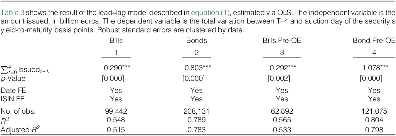
 . We test the significance of the sum of these coefficients. This method is equivalent to the plots of Lou et al. (Reference Lou, Yan and Zhang2013) or Beetsma et al. (Reference Beetsma, Giuliodori, de Jong and Widijanto2016), who look at confidence intervals around the sum of these coefficients. Results are shown in the first 2 columns of Table 3.

TABLE 3 Long description
The table consists of four columns labeled 1 through 4. Column 1 is Bills, Column 2 is Bonds, Column 3 is Bills Pre-Q E, and Column 4 is Bond Pre-Q E.
* The first row shows the summation of Issued sub t plus k from t equals 0 to 4. The values are 0.290 for Bills, 0.803 for Bonds, 0.292 for Bills Pre-Q E, and 1.078 for Bond Pre-Q E. All values are marked with three asterisks indicating statistical significance.
* The p-Value row shows 0.000 for Bills, 0.000 for Bonds, 0.002 for Bills Pre-Q E, and 0.000 for Bond Pre-Q E.
* Date F E and I S I N F E rows are marked Yes for all four columns.
* Number of observations are 99,442 for Bills, 208,131 for Bonds, 62,892 for Bills Pre-Q E, and 121,075 for Bond Pre-Q E.
* R-squared values are 0.548, 0.789, 0.565, and 0.804 respectively.
* Adjusted R-squared values are 0.515, 0.783, 0.533, and 0.798 respectively.
We can see that the total yield increase after announcing the issuance of a T-bill is 0.290 basis points per billion euro issued (column 1), much less than for bonds, whose coefficient stands at 0.803 basis points per billion euro issued. If we stop our sample before January 2015, date at which the ECB and euro-area central banks started to buy government bonds (and virtually no bills) in large amounts, the coefficient for bills remains nearly unchanged, but the coefficient for bonds increases significantly to 1.078 basis points per billion issued, more than three times the coefficient for bills (columns 3 and 4). This larger price impact prior to 2015 is intuitive considering the absence of a large bond buyer such as the central bank.Footnote 10 Given that central banks slowed down or stopped purchasing bonds in 2022, estimates on the pre-QE sample may be more informative for present and future debt management practices than estimates on the full sample.
Even if part of the effect we measure is transitory (especially for bills), the Treasury transacts in the (primary) bond market on day 0 and thus incurs the cost of the full increase we detect between announcement and issuance. The presence of time fixed effects probably leads to ignoring the impact that securities issuance has on similar securities on the same day. We address this issue in Section IV.F. We also run our regressions using issuance in percentage of GDP and in proportion to the outstanding amount of the security, as opposed to billions of euros. Results are shown in Section E of the Supplementary Material. The difference in bills and bonds is then more than 1 to 3 in the full sample and nearly 1 to 4 in the pre-QE period. However, we are primarily interested in the financing of the Treasury and in comparing our estimates to the literature. In the rest of this article, we therefore focus on issuance impact per billion euros issued.
Crucially, we show in our robustness section that if we run the baseline excluding the periods of stress such as the global financial crisis (GFC) and COVID-19, the difference between the price impact of bills and the price of bonds grows to 1 to 5. Thus, we are confident that our results are not driven by years of crises when one could suspect that the demand for safe assets would lower the price impact of bills.
Lastly, it is important to stress that announcements for bills contain a range for each individual security, while announcement for bonds contain a range for the aggregate amount of all three bonds to be issued the following week, leaving more room to the Treasury to adjust issuance amount between announcement and auction day. We will show in the next subsection that neutralizing this strategic behavior only accentuates the difference in the price impact of bonds versus bills. Still, we acknowledge that relatively more (resp. less) information is revealed for bonds than for bills on auction (resp. announcement) day. However, Figure 6 shows that most, if not all, of the effect on bond yields appears before auction day, and that the yield impact on auction day is in fact nearly insignificant. This suggests that the minor difference in the information revelation process cannot explain why bond yields react more than bill yields.
D. Reverse Causality
One may suspect some reverse causality. For instance, the French DMO may issue systematically more bonds if there is a limited increase in the yields after its announcements. This would bias our coefficients toward 0. This phenomenon recalls the challenge faced in the QE literature, when central banks may buy securities that react the least to their purchases (Arrata, Nguyen, Rahmouni-Rousseau, and Vari (Reference Arrata, Nguyen, Rahmouni-Rousseau and Vari2020), Koijen, Koulischer, Nguyen, and Yogo (Reference Koijen, Koulischer, Nguyen and Yogo2021)). However, in the French debt issuance context, we have the advantage of knowing exactly when and what the market learns about the sale. We use this feature in two ways.
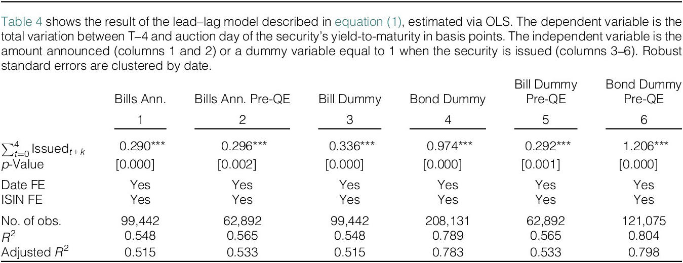
One way to neutralize the behavior of the DMO between the announcement and the actual auction is to use the range of the amount to be issued, which is communicated to the market when it announces which security it will issue. This range is unfortunately only available for bills on an ISIN-by-ISIN basis. We thus replace our independent variable with the middle of the range announced for each T-bill. The results are displayed in columns 1 and 2 of Table 4. These are close, if not identical coefficients, to our baseline.

TABLE 4 Long description
The table consists of 6 columns of results.
Header Row 1: Columns are numbered 1 through 6.
Header Row 2: 1 Bills Ann., 2 Bills Ann. Pre-Q E, 3 Bill Dummy, 4 Bond Dummy, 5 Bill Dummy Pre-Q E, 6 Bond Dummy Pre-Q E.
Row 1 (Summation of Issued sub t plus k from t equals 0 to 4):
- Column 1: 0.290***
- Column 2: 0.296***
- Column 3: 0.336***
- Column 4: 0.974***
- Column 5: 0.292***
- Column 6: 1.206***
Row 2 (p-Value):
- Column 1: [0.000]
- Column 2: [0.002]
- Column 3: [0.000]
- Column 4: [0.000]
- Column 5: [0.001]
- Column 6: [0.000]
Row 3 (Date F E): Yes for all columns.
Row 4 (I S I N F E): Yes for all columns.
Row 5 (No. of obs.):
- Column 1: 99,442
- Column 2: 62,892
- Column 3: 99,442
- Column 4: 208,131
- Column 5: 62,892
- Column 6: 121,075
Row 6 (R-squared):
- Column 1: 0.548
- Column 2: 0.565
- Column 3: 0.548
- Column 4: 0.789
- Column 5: 0.565
- Column 6: 0.804
Row 7 (Adjusted R-squared):
- Column 1: 0.515
- Column 2: 0.533
- Column 3: 0.515
- Column 4: 0.783
- Column 5: 0.533
- Column 6: 0.798
In order to look at bonds, we run regressions where instead of using the amounts issued as the right-hand side variables, we employ a dummy equal to 1 when the ISIN is re-issued, and 0 otherwise. In this way, we measure the impact of an average issuance, which is dictated by long-term budgetary considerations rather than the effect of a specific issuance, which may be strategic. This second strategy is similar to Lou et al. (Reference Lou, Yan and Zhang2013), even if there are important differences due to the institutional setup, notably re-issuances. We employ the same method with bills for comparison.
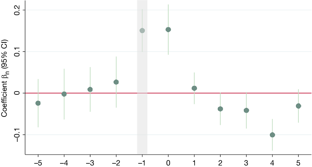
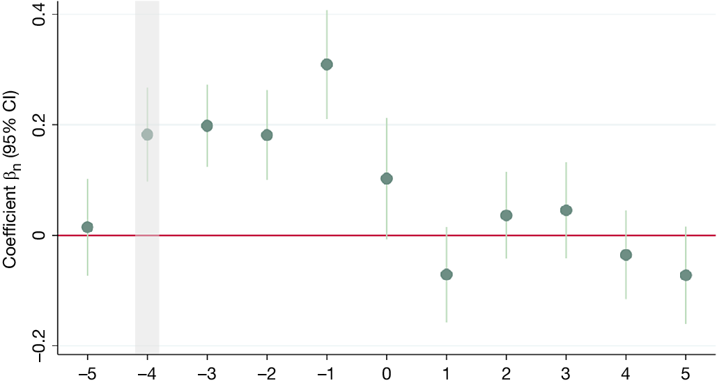
The coefficient plots for regressions using dummy variables are shown in Figures 7 and 8, and display similar patterns as per-billion auction. Coefficients are divided by 1.89, the average size of an auction in billions of euros for comparison with the baseline. The pattern for bonds seems somehow cleaner, with a nearly exact same increase at T–4, T–3, and T–2.
Figure 7 plots the yield change (in basis points) on each day prior to and after the issuance of a specific security (defined at the ISIN level). Auction day is day 0. The shaded areas mark announcement day (T–1 for bills and T–4 for bonds). Issuance is defined as a dummy variable equal to 1 when there is an issuance, and 0 otherwise. Coefficients are then divided by the average size of an auction (1.89 billion euro) to make these coefficients directly comparable to the baseline.

FIGURE 7 Long description
The x-axis represents days relative to the auction day 0, ranging from minus 5 to 5. The y-axis represents Coefficient beta sub n 95 percent C I, ranging from minus 0.1 to 0.2. A horizontal red line is fixed at 0.
Data points are represented by green circles with vertical error bars indicating the 95 percent confidence interval.
* From day minus 5 to minus 2, coefficients are near zero with wide error bars crossing the red line.
* A vertical light gray shaded area highlights day minus 1, the announcement day, where the coefficient rises significantly to approximately 0.15.
* On day 0, the auction day, the coefficient remains high at approximately 0.16.
* From day 1 to day 5, the coefficients drop back toward or below zero. Day 4 shows a notable dip to approximately minus 0.1 before returning toward zero on day 5.
Figure 8 plots the yield change (in basis points) on each day prior to and after the issuance of a specific security (defined at the ISIN level). Auction day is day 0. The shaded areas mark announcement day (T–1 for bills and T–4 for bonds). Issuance is defined as a dummy variable equal to 1 when there is an issuance, and 0 otherwise. Coefficients are then divided by the average size of an auction (1.89 billion euro) to make these coefficients directly comparable to the baseline.

FIGURE 8 Long description
The Y-axis is labeled Coefficient beta sub n open parenthesis 95 percent C I close parenthesis, with a scale from minus 0.2 to 0.4. A horizontal red line marks the zero baseline. The X-axis represents a timeline of discrete events from minus 5 to 5.
Data points are represented by green circles with vertical error bars indicating the 95 percent confidence interval.
* At minus 5, the coefficient is near zero.
* A vertical gray shaded band highlights the period at minus 4, where the coefficient rises to approximately 0.18.
* From minus 3 to minus 2, the coefficients remain elevated near 0.2.
* At minus 1, the coefficient peaks at approximately 0.3.
* At 0, the coefficient drops to 0.1.
* At 1, the coefficient falls below the zero line to approximately minus 0.08.
* From 2 to 3, the coefficients rise slightly above zero.
* At 4 and 5, the coefficients fall back below the zero line to approximately minus 0.05.
Table 4 shows in columns 3 and 4 the daily increases in the yields of bills and bonds, respectively, cumulated over the 4 days preceding the auction, for the whole sample. Coefficients are slightly higher than in the case of the baseline, suggesting a small bias toward 0 in the baseline. Yields on bonds are still found to react by around three times as much as for bills, at 0.974 basis points versus 0.336. The difference between bills and bonds increases during the pre-QE period, where the coefficient on the latter is more than four times larger than the coefficient on the former (0.292 vs. 1.206) as shown in columns 3 and 4.
Overall, results of Table 4 suggest that there is little if no systematic change in the plans of the DMO between the announcement and the actual auction, but that in any case bonds react more strongly to additional supply than bills. In theory, the market could be anticipating the issuance of a given security, even before it is announced, which would again lead us to underestimate the impact of issuances on yields, as part of the increase would already be priced in when the announcement comes. However, there is at one point in time a comparable number of bills, medium-term bonds, and long-term bonds, around 20 of each type (see Figure 3 in the Supplementary Material), and thus there is no reason that one category of securities could be better anticipated than another ahead of the auctions dedicated to that type of security. While slightly more information is revealed for bonds on auction days (the range to be issued is available only for bills), most, if not all, of the yield increase occurs prior to the auction, especially for bonds, suggesting that most of the effect comes from whether a bond will be re-issued or not. Information revealed on auction day, such as how much is actually issued, seems to play little if no role.
E. The Role of Duration Risk
Standard intuition would suggest that bond supply raises yields because it increases the amount of duration risk that the market has to bear, the exact opposite of QE (Greenwood and Vayanos (Reference Greenwood and Vayanos2014)). One way to look at this question is by examining the spread between the yield of a security of a specific maturity and the OIS rates of the same maturity, a measure of the asset swap spread. OIS should carry both expectations of future interest rates and the price of duration risk, that is, the term premium in euros. If increases in the supply of bonds raise their yields through a change in the term premium, the yield-OIS spread should not react to news of future issuance. OIS are among the most liquid euro-denominated fixed income instruments and are used in the context of high-frequency identification (Altavilla, Brugnolini, Gürkaynak, Motto, and Ragusa (Reference Altavilla, Brugnolini, Gürkaynak, Motto and Ragusa2019)).
We construct daily swap curves from standard OIS maturities retrieved from Bloomberg. Using the Nelson–Siegel–Svensson model, we compute the term structure for each day at 1-month interval and match these monthly nodes of the swap curve with each security based on its residual maturity. We then run our baseline regressions using the asset swap spread on the left-hand side and billion issued on the right-hand side with day and ISIN fixed effects.
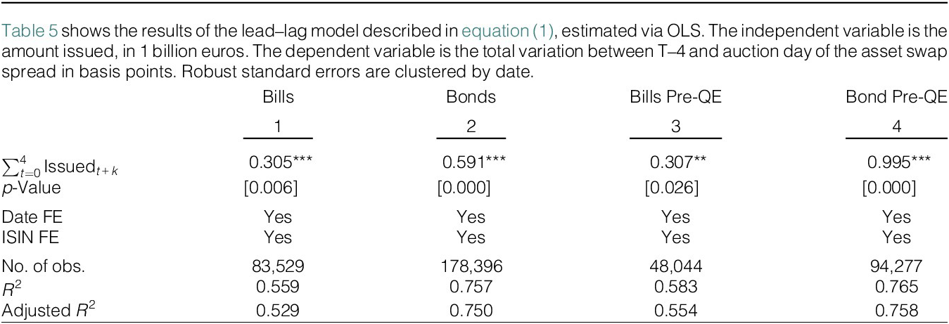
Results are shown in Table 5. For comparisons, we run regressions on the same sample (Table 3 in the Supplementary Material) given that OIS were not available in the early days of the euro area. As expected, coefficients drop for bonds but remain positive, significant, and larger than for bills. In the pre-QE period, 1 billion issuance increases the asset swap spread by 0.995 basis points, which is slightly less than the 1.16 basis points for bond yields (column 4 of Table 3 in the Supplementary Material) but remains really close. This suggests that most of the effect of issuance on yields does not come from a rise in the term premium, which is the price of duration risk (Vayanos and Vila (Reference Vayanos and Vila2021)).

TABLE 5 Long description
The table consists of four columns numbered 1 through 4.
Column 1: Bills.
Column 2: Bonds.
Column 3: Bills Pre-Q E.
Column 4: Bond Pre-Q E.
Row 1: Summation from t equals 0 to 4 of Issued sub t plus k. Values are 0.305 with three asterisks for Bills, 0.591 with three asterisks for Bonds, 0.307 with two asterisks for Bills Pre-Q E, and 0.995 with three asterisks for Bond Pre-Q E.
Row 2: p-Value. Values in brackets are 0.006, 0.000, 0.026, and 0.000 respectively.
Row 3: Date F E. All columns are marked Yes.
Row 4: I S I N F E. All columns are marked Yes.
Row 5: Number of observations. Values are 83,529, 178,396, 48,044, and 94,277 respectively.
Row 6: R-squared. Values are 0.559, 0.757, 0.583, and 0.765 respectively.
Row 7: Adjusted R-squared. Values are 0.529, 0.750, 0.554, and 0.758 respectively.
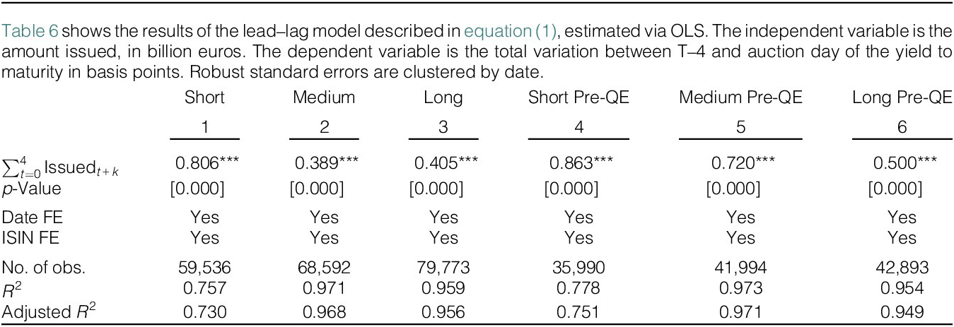
To confirm that all the bond yields’ increases do not come only from the term premium, we run our regressions on a subsample of bonds of different maturities. We cut our bond sample into three, according to residual maturity. We call “short” bonds all those with less than 3-year of residual maturity, the standard maturity for the shortest bonds issued by the French Treasury. We then call “medium” bonds those between 3 and 8 years of residual maturity, thus capturing the standard 5-year bond but not any 10-year bond issued in previous years. Lastly, the “long” bonds category includes all bonds with residual maturity of 8 years or more. These thresholds at standard maturities allow to have a comparable number of observations in each bucket. Results of these regressions for the whole sample and the pre-QE period are displayed in Table 6.

TABLE 6 Long description
The table consists of six columns numbered 1 through 6. The columns are: 1 Short, 2 Medium, 3 Long, 4 Short Pre-Q E, 5 Medium Pre-Q E, and 6 Long Pre-Q E.
Row 1: Summation of Issued sub t plus k from t equals 0 to 4. Values are 0.806, 0.389, 0.405, 0.863, 0.720, and 0.500. All values are marked with three asterisks indicating significance.
Row 2: p-Value. All columns show 0.000 in brackets.
Row 3: Date F E. All columns show Yes.
Row 4: I S I N F E. All columns show Yes.
Row 5: Number of observations. Values are 59,536; 68,592; 79,773; 35,990; 41,994; and 42,893.
Row 6: R-squared. Values are 0.757, 0.971, 0.959, 0.778, 0.973, and 0.954.
Row 7: Adjusted R-squared. Values are 0.730, 0.968, 0.956, 0.751, 0.971, and 0.949.
One can see that actually the effect of issuance on bond yields does not increase with maturity, but quite the opposite, especially in the pre-QE period. In the full-sample regressions, the effect of issuance for the shortest maturity bonds is nearly twice as large as for the longest maturity bonds (columns 1 and 3 of Table 6). Moreover, the bonds most affected by QE seem to be those of medium maturity (columns 2 and 5). This makes sense given that ECB QE portfolio for France had a weighted average maturity between 6 and 7 years, suggesting heavy purchase on that segment.Footnote 11 This result is all the more surprising because the so-called “short” bonds are not some very old and illiquid securities recently re-issued. On average, the initial maturity of old bonds is 7 years, compared to 9.7 years for “medium” bonds and 25.2 years for “long” bonds.
Such a pattern is consistent with the notion of preferred habitat, that is, markets are segmented as some agents want a specific asset with specific maturity to match their needs. Demand elasticity may not decrease monotonously with duration risk as would be the case in the absence of preferred habitat, with agents willing to bear only limited duration risk (Vayanos and Vila (Reference Vayanos and Vila2021)).Footnote 12 In Section V, we will present evidence that bonds are indeed held by investors who may have specific needs along the yield curve, while bill investors may care less about maturity.
Incidentally, the secondary role played by duration risk suggests that primary dealers are not the only force behind the price dynamics we observe around auctions. Dealers have no reason to be attached to specific points of the yield curve and should only try to avoid taking excessive duration risk with their inventories, as explained by Fleming, Nguyen, and Rosenberg (Reference Fleming, Nguyen and Rosenberg2024). In line with Jansen, Li, and Schmid (Reference Jansen, Li and Schmid2024), we classify primary dealers as risk-averse arbitrageurs in the sense of Vayanos and Vila (Reference Vayanos and Vila2021), at least when it comes to their own inventory holdings. We thus conclude that at least part of the impacts we observe is due to the presence of preferred habitat investors.
F. Spillover from Other Securities Issuance
Up to now, we have focused on the effect of issuance on a security’s own yield. However, in the presence of preferred habitat and limited risk-bearing capacity, supply and demand shocks should have effects on other securities of similar maturity (Selgrad (Reference Selgrad2023), Ray et al. (Reference Ray, Droste and Gorodnichenko2024)). Such interactions are particularly important in the context of French Treasury auctions where three of four securities of the same type (bonds or bills) are issued on the same day.
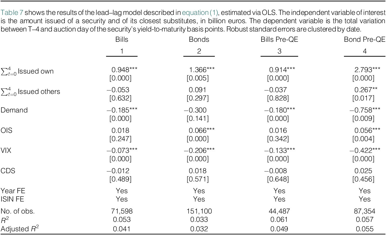
In order to control for cross-security spillovers, we add as explanatory variables the issued amount of all securities of the same type (all bonds and all bills) on those days. This requires removing date fixed effects. We use year fixed effects instead to control for changes in GDP, the general price level, and the fiscal deficit.Footnote 13
Because we do not have high-frequency controls for the demand of bonds and bills in the form of date fixed effects, we include the total amount of bids at auctions for each ISIN. This is very close to Ray et al. (Reference Ray, Droste and Gorodnichenko2024) or Kacperczyk et al. (Reference Kacperczyk, Pérignon and Vuillemey2021) who use the bid-to-cover ratio. We just include the numerator and denominator separately. Like them, we assume that demand impacts the market when it is revealed, on auction day. We also control for other important high-frequency variables, such as changes to the term structure of interest rates using OISs for each maturity, general risk aversion using the VIX, and credit risk using the 5-year Credit Default Swap (CDS) on France. All these control variables are taken in first difference, just like yields.
Results are shown in Table 7. In general, coefficients for “own issuance” are significantly larger than for regressions with date fixed effects. In the pre-QE period, bond issuance impact yields by 2.793 basis points. Like in the baseline, this number is between three and four times larger than the impact on bills (0.914 basis points). Once again, we find that QE had little effect on bills but a large impact on bonds, with the yield impact nearly two times as large during the period where the central bank is absent compared to the full sample (columns 2 and 4).

TABLE 7 Long description
The table consists of four columns labeled 1 through 4, representing Bills, Bonds, Bills Pre-Q E, and Bond Pre-Q E respectively.
Row-by-row data:
- Summation of t equals 0 to 4 Issued own: Column 1 is 0.948*** [0.000]; Column 2 is 1.366*** [0.005]; Column 3 is 0.914*** [0.000]; Column 4 is 2.793*** [0.000].
- Summation of t equals 0 to 4 Issued others: Column 1 is -0.053 [0.632]; Column 2 is 0.091 [0.297]; Column 3 is -0.037 [0.828]; Column 4 is 0.267** [0.017].
- Demand: Column 1 is -0.185*** [0.000]; Column 2 is -0.300 [0.141]; Column 3 is -0.180*** [0.000]; Column 4 is -0.758*** [0.009].
- O I S: Column 1 is 0.018 [0.247]; Column 2 is 0.066*** [0.000]; Column 3 is 0.016 [0.342]; Column 4 is 0.056*** [0.004].
- V I X: Column 1 is -0.073*** [0.000]; Column 2 is -0.206*** [0.000]; Column 3 is -0.133*** [0.000]; Column 4 is -0.422*** [0.000].
- C D S: Column 1 is -0.012 [0.489]; Column 2 is 0.018 [0.571]; Column 3 is -0.008 [0.648]; Column 4 is 0.025 [0.456].
- Year F E: Yes for all columns.
- I S I N F E: Yes for all columns.
- Number of observations: Column 1 is 71,598; Column 2 is 151,100; Column 3 is 44,487; Column 4 is 87,354.
- R-squared: Column 1 is 0.053; Column 2 is 0.033; Column 3 is 0.061; Column 4 is 0.057.
- Adjusted R-squared: Column 1 is 0.041; Column 2 is 0.032; Column 3 is 0.049; Column 4 is 0.055.
As expected, demand (measured by the total amount of bids) is negatively signed and OIS is positive and significant for bonds. CDS is not significant, while VIX is. These two coefficients suggest that France benefited from safe-haven flows in times of stress as yields reacted negatively to market-wide stress (VIX) and was not sensitive to France’s perceived sovereign risk (CDS). We discuss further the role of crisis periods in our robustness section.
The overall increase in the coefficient associated with a security’s own issuance suggests that date fixed effects absorb large portions of the change in yields in a given day. This is most likely because date fixed effects suppressed the average increase of all bond (resp. bill) yields on a given auction day. Removing date fixed effects and replacing them by our high-frequency controls, and in particular OIS rates of the same maturity, allows us to have a more precise estimate of the increase in yields following a surprise issuance.
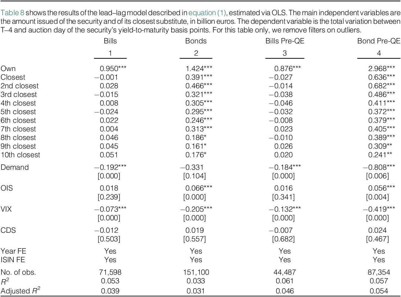
However, the coefficient associated with the issuance of other securities is in general not significant. How can this be? We show in Table 8 that one needs to take a more granular approach to capture spillovers.

TABLE 8 Long description
The table presents O L S regression results for four models labeled 1 through 4.
Column headers are:
1. Bills
2. Bonds
3. Bills Pre-Q E
4. Bond Pre-Q E
Row-wise data for ‘Own’ issuance shows positive coefficients across all models: 0.950, 1.424, 0.876, and 2.968, all significant at the 0.01 level.
For ‘Closest’ to ‘10th closest’ substitutes:
- Bills (Model 1) and Bills Pre-Q E (Model 3) show mostly non-significant, near-zero coefficients.
- Bonds (Model 2) and Bond Pre-Q E (Model 4) show consistently positive and significant coefficients ranging from 0.161 to 0.682.
Control variables include:
- Demand: Negative coefficients across all models, significant except for Model 2.
- O I S: Positive and significant for Bonds (0.066) and Bond Pre-Q E (0.056).
- V I X: Negative and significant across all models, ranging from -0.073 to -0.419.
- C D S: Non-significant across all models.
Fixed Effects (F E) for Year and I S I N are included (‘Yes’) for all models.
Model Statistics:
- Number of observations: 71,598 (Model 1); 151,100 (Model 2); 44,487 (Model 3); 87,354 (Model 4).
- R-squared values range from 0.033 to 0.061.
- Adjusted R-squared values range from 0.031 to 0.054.
More specifically, we do not test for the total amount of bonds (resp. bills) being issued but rather for the issuance of the closest ones in terms of maturity. For each bond (resp. bills), we select the two bonds that are the closest in terms of maturity: one with higher maturity and one with lower maturity, thus one bond is in “between” its two closest bonds. Then, we select the second closest ones and so on. For each security, we select 10 pairs of bonds and take the sum of the issued amount of these two bonds.
As shown in columns 2 and 4 of Table 8, the impact of issuance of securities of similar maturity on a bond yield is positive, significant, and generally decreases with their distance to the bond on the yield curve. In fact, with the exception of the 2nd and the 7th closest securities for the whole sample and of the 3rd and 5th closest securities for the pre-QE sample, the impact of issuance decreases monotonously with the distance on the yield curve. Significance decreases monotonously for the 10 pairs in all cases.
For bills, the issuance of neighboring securities has no impact. This makes sense, as T-bills have by construction low duration risk and are close substitutes for cash. For that reason, one should expect the influence of preferred habitat investors on T-bills to be less pronounced. This is in line with the theory of Vayanos and Vila (Reference Vayanos and Vila2021) which states that when there is no constraint to arbitrage, preferred habitat investors have no impact. This is also in line with the mechanisms and elasticities found in Jansen et al. (Reference Jansen, Li and Schmid2024).Footnote 14 This is evidence that bond market investors are more attached to specific maturity points on the yield curve, while T-bill investors do not care much about maturity, given that they are anyway fairly short.Footnote 15 Moreover, these results also show that the issuance of one bond impacts the yield of other bonds, suggesting that bond yields are not determined in isolation, which would happen if there were only preferred habitat investors in the market without any risk-averse arbitrageurs. We thus conclude that the two types of agents are present in the French debt market.
Incidentally, removing date fixed effects enables us to identify larger impacts (3.06 basis points) but is very much credible when compared to rest of the literature. For instance, Lou et al. (Reference Lou, Yan and Zhang2013) find that the 5-day increase before auctions in bond yields to be between 2.3 and 4.3 basis points per billion euro issued for U.S. bond auctions. For the United Kingdom, Lengyel (Reference Lengyel2022) finds that issuance shocks cause 0.8 to 1.2 basis points increase in yields per billion euro issued.Footnote 16
G. Robustness
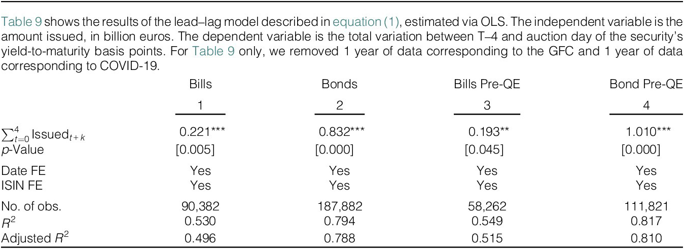
The first and most important test to demonstrate the solidity of our results is to run our regressions taking out periods of acute crises, which one may suspect to be the driver of the low impact of bills issuance on yields, as governments could exploit safe asset demand in times of stress. Thus, we re-run our baseline without the GFC and COVID-19. To avoid using arbitrary dates, we take out all observations for 1 full year starting on Sept. 15, 2008, when Lehman Brothers failed, for the GFC, and 1 full year starting on Mar. 11, 2020, when the WHO characterizes COVID-19 outbreak as a pandemic. Results are shown in Table 9.

TABLE 9 Long description
A table with four columns of data: 1 Bills, 2 Bonds, 3 Bills Pre Q E, and 4 Bond Pre Q E.
Row 1: Summation from t equals 0 to 4 of Issued sub t plus k.
- Bills: 0.221 with three asterisks.
- Bonds: 0.832 with three asterisks.
- Bills Pre Q E: 0.193 with two asterisks.
- Bond Pre Q E: 1.010 with three asterisks.
Row 2: p-Value.
- Bills: open bracket 0.005 close bracket.
- Bonds: open bracket 0.000 close bracket.
- Bills Pre Q E: open bracket 0.045 close bracket.
- Bond Pre Q E: open bracket 0.000 close bracket.
Row 3: Date F E. All columns show Yes.
Row 4: I S I N F E. All columns show Yes.
Row 5: Number of observations.
- Bills: 90,382.
- Bonds: 187,882.
- Bills Pre Q E: 58,262.
- Bond Pre Q E: 111,821.
Row 6: R squared.
- Bills: 0.530.
- Bonds: 0.794.
- Bills Pre Q E: 0.549.
- Bond Pre Q E: 0.817.
Row 7: Adjusted R squared.
- Bills: 0.496.
- Bonds: 0.788.
- Bills Pre Q E: 0.515.
- Bond Pre Q E: 0.810.
Table 9 shows results extremely close to the baseline, and in fact the difference between bills and bonds is slightly larger when crisis observations are removed. In the pre-QE period, the coefficient for bonds is now more than five times larger than the coefficient for bills. In Table 4 in the Supplementary Material, we show that if we are even more conservative and take out the full years 2008, 2009, 2020, and 2021, the conclusion is the same. That is, the gap we have shown between bills and bonds in terms of price impact at issuance is in fact slightly larger than in the baseline and we can thus be confident that it is not at all a by-product of crisis years.
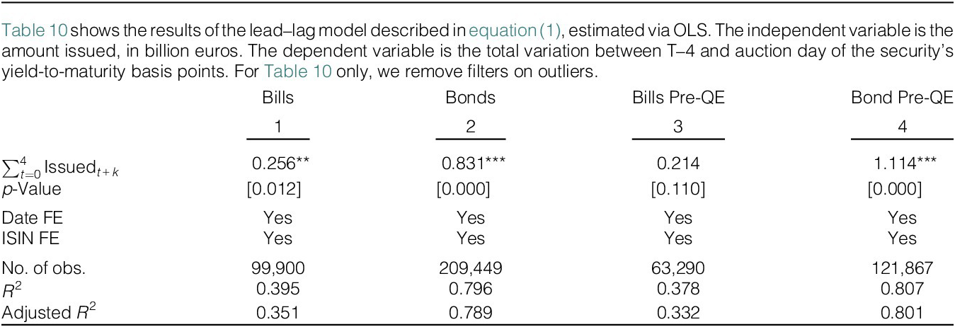
In our second robustness test, we run our regressions but this time including outliers, that is, including the 0.5% of observations on each side of the distribution that were previously removed. Results are shown in Table 10. Once again, the difference between bills and bonds in terms of coefficient size and significance tends to grow, and is more than 1 to 5 in the pre-QE period. If anything, this result stresses the conservativeness of our baseline when estimating the difference in the price impact of bills versus bonds.

TABLE 10 Long description
The table consists of four columns of data labeled 1 through 4. Column 1 is Bills, Column 2 is Bonds, Column 3 is Bills Pre-Q E, and Column 4 is Bond Pre-Q E.
* The first row shows the summation of Issued sub t plus k from t equals 0 to 4. The values are: 0.256 with two asterisks for Bills, 0.831 with three asterisks for Bonds, 0.214 for Bills Pre-Q E, and 1.114 with three asterisks for Bond Pre-Q E.
* p-Value row: Bills [0.012], Bonds [0.000], Bills Pre-Q E [0.110], Bond Pre-Q E [0.000].
* Date F E row: Yes for all four columns.
* I S I N F E row: Yes for all four columns.
* Number of observations: Bills 99,900; Bonds 209,449; Bills Pre-Q E 63,290; Bond Pre-Q E 121,867.
* R-squared: Bills 0.395, Bonds 0.796, Bills Pre-Q E 0.378, Bond Pre-Q E 0.807.
* Adjusted R-squared: Bills 0.351, Bonds 0.789, Bills Pre-Q E 0.332, Bond Pre-Q E 0.801.
V. Who Are the Preferred Habitat Investors?
In previous sections, we showed that bills and bonds react differently to supply shocks, a pattern consistent with the presence of preferred habitat investors. In this section, we shed some light on who these different investors are and why they may prefer bonds over bills or vice versa.
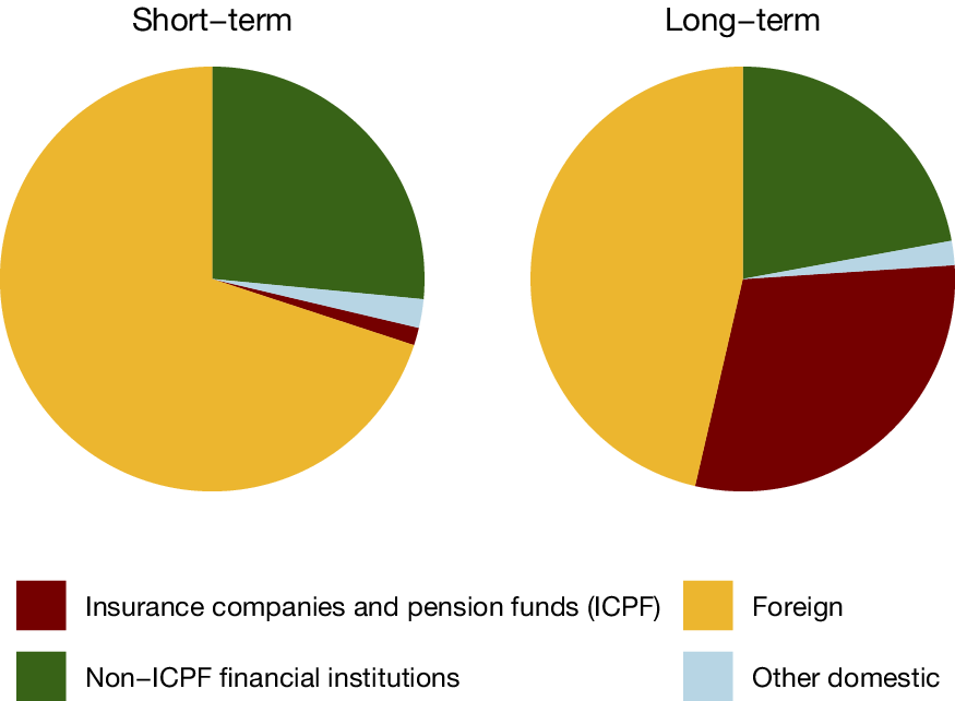
We start our investigation by looking at the ECB securities holdings statistics (SHS) database. This data set gives information for each government securities market of the euro area and splits holders for bills and for bonds separately since 2013. Holders are grouped by categories such as insurance companies and pension funds (ICPF), monetary and financial institutions (Banks), nonresidents, and others. We graph the investor base (excluding the Eurosystem) in Figure 9. The graph reveals stark differences. While ICPF are the single largest holders of French bonds, they represent only a modest fraction of T-bills outstanding. The latter category of securities is largely held by foreign institutions.
Figure 9 shows non-ICPF financial institutions, including banks and all non-foreign financial institutions such as mutual funds. Foreign includes all nonresidents (public and private). Other domestic includes nonfinancial corporations and households. Source: ECB’s securities holdings statistics (SHS) and quarterly sector accounts (QSA) statistics. Average over 2013 (first observations) to 2020. Eurosystem purchases under the public sector purchase program (PSPP) have been excluded using ECB monthly reporting.

FIGURE 9 Long description
The y-axis is labeled Coefficient beta sub n 95 percent C I, with a scale from minus 0.2 to 0.4. A horizontal red line marks the zero baseline. The x-axis ranges from minus 5 to 5 in integer increments.
Data points are represented by green circles with vertical error bars.
* At minus 5, the point is near 0.
* At minus 4, which is highlighted by a vertical gray shaded bar, the point rises to approximately 0.18.
* At minus 3 and minus 2, points remain elevated near 0.2.
* At minus 1, the coefficient peaks at approximately 0.3.
* At 0, the point drops to 0.1.
* At 1, the point falls below the zero line to approximately minus 0.08.
* At 2 and 3, points return to slightly above zero.
* At 4 and 5, points fall back below the zero line to approximately minus 0.05 and minus 0.08 respectively.
Confidence intervals are widest at minus 1 and 0, and narrowest at minus 5.
The presence of ICPF in the bond market is noteworthy as their preferred habitat behavior has been widely recognized in the literature. On the theoretical front, Vayanos and Vila (Reference Vayanos and Vila2021) use pension funds to exemplify preferred habitat investors. On the empirical side, Koijen et al. (Reference Koijen, Koulischer, Nguyen and Yogo2021) or Arrata et al. (Reference Arrata, Nguyen, Rahmouni-Rousseau and Vari2020) show that asset purchase programs have a greater impact on yield or repo rates when ICPFs are present, stressing their price inelasticity. Jansen et al. (Reference Jansen, Li and Schmid2024) show a similar result for the U.S. bond market. Symmetrically, it is plausible to think that securities held mostly by this type of investors should see a greater price impact when they are issued.
ICPF may have different demand curves at different maturity points, and it may not be possible to know a priori how demand changes with duration. In the short run, they cannot expand their balance sheet beyond the insurance premia they receive from customers, a sticky flow. Kubitza (Reference Kubitza2026) shows empirically that premia payments significantly move the bond demand of insurance companies. Moreover, ICPF have strict duration targets they need to adhere to. Investing in assets of duration higher or lower than their liabilities exposes them to a maturity mismatch (Guibaud, Nosbusch, and Vayanos (Reference Guibaud, Nosbusch and Vayanos2013)). The duration of their portfolios is also heavily influenced by regulation (Greenwood and Vissing-Jorgensen (Reference Greenwood and Vissing-Jorgensen2019), Jansen (Reference Jansen2025)).
The situation for T-bill investors is radically different. The share of ICPF in the holding structure of short-term debt is significantly lower than for long-term debt. Conversely, the share of foreign investors is significantly higher. Foreign investors may be private or public, such as foreign central banks. The crucial role of foreign investors in the U.S. Treasury market and other government bond markets has been stressed by Somogyi, Wallen, and Xu (Reference Somogyi, Wallen and Xu2025).
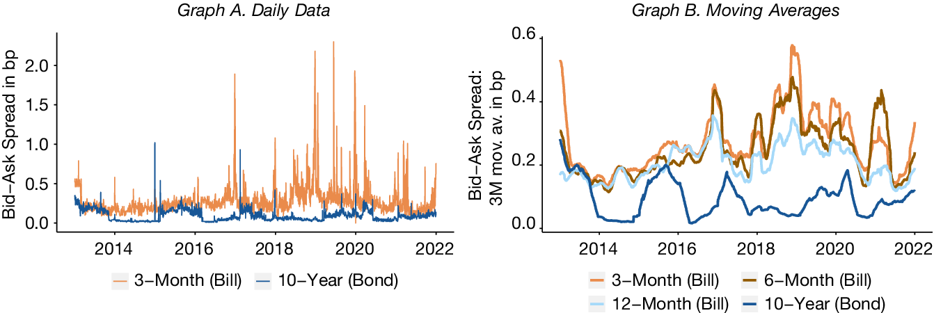
Why do foreign investors hold French Treasury bills? A natural argument is that bills are supposed to be more liquid on the secondary market than bonds (e.g., Nagel (Reference Nagel2016)). However, we show in Figure 10 that French T-bills are in general less liquid than bonds when using the standard bid–ask spread measure. Indeed, one can see that bid–ask spreads for bills are in general higher than for bonds (Figure 10) and the 1-year tenor is consistently the most liquid of the bills.
Figure 10 plots the bid–ask spread for the on-the-run 3-month and 10-year security issued by the French government. 3.b plot uses 3-month moving average for all French on-the-run T-bills (3-, 6-, and 12-month initial maturity). Using moving average smooths out volatility and allows to plot more securities while keeping the graph readable. Source: Bloomberg.

FIGURE 10 Long description
The figure consists of two panels.
Left panel titled Short-term. The pie chart shows four segments. Starting from the top and moving clockwise, a dark green segment representing Non-I C P F financial institutions occupies approximately one-quarter of the chart. A very thin light blue segment for Other domestic and a sliver of dark red for Insurance companies and pension funds I C P F follow. The remaining majority, roughly two-thirds of the chart, is a large yellow segment representing Foreign investors.
Right panel titled Long-term. The pie chart shows a different distribution. The dark green segment for Non-I C P F financial institutions remains at approximately one-quarter. A thin light blue segment for Other domestic follows. The dark red segment for I C P F is significantly larger here, occupying nearly one-third of the chart. The yellow Foreign segment is reduced compared to the short-term chart, making up the remaining portion of slightly less than half.
Legend at the bottom.
Left column. Dark red square for Insurance companies and pension funds I C P F. Dark green square for Non-I C P F financial institutions.
Right column. Yellow square for Foreign. Light blue square for Other domestic.
This suggests that it may actually be more expensive to buy and sell a bill on the secondary market than a bond, contrary to the standard intuition from the safe assets literature. This feature may not be specific to France and has been hinted at in the case of the United States some time ago by Fleming (Reference Fleming2001), who showed T-bill bid–ask spreads to be higher than for bonds, and trading frequency to be higher for the latter category of securities.Footnote 17 This incidentally shows that our results cannot simply be explained by differences in secondary market liquidity. It is possible that this phenomenon is related to bid–ask spreads generally widening (in yield terms) as securities approach maturity, as documented by Fleming (Reference Fleming2002).
It must therefore be noted that the main feature of bills and the reason they are sought after is not their secondary market liquidity but, more probably, their low interest and credit risk. Foreign investors may need to redeploy any cash inflows, coming from the sale or the payment from an asset in safe cash-like assets like repo or Treasury bills. Foreign central banks need to receive steady inflows of cash to be able to intervene on the FX market and may thus be looking for assets with redemption liquidity. They may accumulate a T-bill portfolio with staggered repayments to get cash regularly.
To be sure, France during our period of study redeemed one bill every week and was considered safe. As can be seen in Figure 11, French and German T-bills showed similar flight-to-safety properties during the pandemic, at the opposite of Spain and Italy. Logically, the IMF Sovereign Debt Investor Base for Advanced Economies reveals that an average of 17% of French debt is held by foreign central banks, compared to just 9% for Spain and 5% for Italy.
Figure 11 plots the yield-to-maturity of 3-month (thick lines) and 12-month (dashed lines) T-bills for the four largest euro-area countries. Each color corresponds to a country. Source: Bloomberg.

FIGURE 11 Long description
The figure consists of two panels.
Graph A, titled Daily Data, features a horizontal x-axis representing years from 2014 to 2022 and a vertical y-axis labeled Bid-Ask Spread in b p, ranging from 0.0 to 2.0. It plots two datasets. The 3-Month Bill, shown in orange, exhibits high volatility with several sharp spikes reaching above 1.5 b p, particularly around 2017, 2019, and 2020. The 10-Year Bond, shown in dark blue, remains relatively stable near 0.2 b p, with one notable spike near 1.0 b p in 2015.
Graph B, titled Moving Averages, uses the same x-axis but a y-axis labeled Bid-Ask Spread 3 M mov. av. in b p, ranging from 0.0 to 0.6. This panel includes four datasets. The 3-Month Bill in orange and 6-Month Bill in brown follow similar fluctuating paths, peaking near 0.5 b p in 2019. The 12-Month Bill in light blue shows a smoother trend, generally staying between 0.1 and 0.3 b p. The 10-Year Bond in dark blue shows the lowest overall spread, frequently dipping toward 0.0 b p between 2014 and 2016 and again in 2017, before rising to fluctuate between 0.1 and 0.2 b p through 2022.
VI. Conclusion
In this article, we documented that when a government needs to raise a large amount of money quickly, it will favor the short-term debt market. This feature of debt management is visible in the data and in statements made by DMOs and Treasury officials. Based on the rich setup offered by French Treasury debt auctions, we have shown empirically, in the largest euro-denominated T-bill market, that indeed short-term debt issuances have a lower price impact than long-term debt issuances. The latter raise yields by four times as much as the former. This difference is not a by-product of crisis times and remains even when several years of crises are removed from the sample. Central bank purchases in the bond market consistently lower the price impact of auctions on yields.
The larger price impact of bond auctions compared to bill auctions cannot be explained only by duration risk. This is evidenced, for instance, by the fact that bonds with relatively short maturity have larger price impacts than longer-term bonds. Asset swap spreads react similarly to bond yields, suggesting that the price of duration risk is not the main driver of our results. Moreover, bond auctions have local effects on bonds of similar maturities, which is consistent with the presence of preferred habitat investors in the market for French debt.
The large share of ICPF in the French bond market corroborates this intuition. Indeed, these categories of investors are largely recognized in the literature as having strong preferences for some segment of the yield curve, and little leeway on how much they can invest at a given point in time. By contrast, T-bill investors are mostly foreign institutions, which are likely to be more flexible and more diverse.
Appendix. Statements from National Debt Management Offices
“Like during previous crises, short-term borrowing is a tool to respond to unexpected shocks on financing needs. In 2020, the stock of [bills] will however remain way below the levels reached during the 2008–2009 crisis.” Agence France Trésor, December 2020.Footnote 18
“A large part of the additional borrowing requirement was financed via securities with maturities of less than 1 year—so-called non-interest-bearing federal Treasury bonds or Bubills. Compared to the original planning from December 2019, the issue volume of these instruments was roughly tripled. During the financial crisis in 2009/2010, the federal government had already used this very flexible instrument to cover its high borrowing requirements.” Bundesfinanzministerium, February 2021.Footnote 19
“The [Treasury Borrowing Advisory] Committee generally agreed that while T-bills would need to act as a shock absorber in the near term, Treasury should increase the supply of [bonds] over time to mitigate the increase in roll over risk.” Treasury Borrowing Advisory Committee, May 2020.
“As the deficit has risen, the US Treasury has found it increasingly hard to finance via long-term debt without causing an uncomfortable rise in borrowing costs. It has boosted the share of short-term debt it issues—but analysts warned it risks hitting the limits of demand.” Financial Times, June 2024.
Supplementary Material
To view supplementary material for this article, please visit http://doi.org/10.1017/S0022109026102993.