

1. Introduction
‘Warming of the climate system is unequivocal, as is now evident from observations of increases in global average air and ocean temperatures’ (IPCC, 2007a). The future accumulation of greenhouse gases is very likely to further exacerbate warming (IPCC, 2007a). It is consequently quite important to understand what will happen as temperatures rise. One of the most critical climate-sensitive sectors is agriculture (IPCC, 2007b). Specifically, agriculture in Africa is of great concern because it is very important to the region's economy, accounting for 13.1 per cent of gross domestic product (GDP) in the continent as a whole and 20.3 per cent in sub-Saharan Africa, compared to 3 per cent for the world economy (World Bank, 2009). Further, hundreds of millions of Africans depend heavily on what is grown locally for food and income. Finally, many parts of Africa are already hot and dry and therefore very vulnerable to further warming (IPCC, 2007b). In this paper, we develop a new approach to valuing the agricultural impacts of climate change using agro-ecological zones (AEZs) across the vast landscape of Africa.
Several methods have been used to measure the impact of climate change on African agriculture (see review by Mendelsohn and Dinar, Reference Mendelsohn and Dinar2009). Crop simulation models have been used to examine the direct effect of climate change on individual crops (Rosenzweig and Parry, Reference Rosenzweig and Parry1994; Parry et al., Reference Parry, Rosenzweig, Iglesias, Livermore and Fischer2004). These studies found that yields of major grains cultivated in Africa would fall precipitously with warming. The Ricardian method uses an empirical cross-sectional approach to measure the relationship between net revenues and climate (Mendelsohn et al., Reference Mendelsohn, Nordhaus and Shaw1994). Ricardian studies in Africa have found that hot and dry climate scenarios would reduce crop net revenues in Africa (Kurukulasuriya et al., Reference Kurukulasuriya and Mendelsohn2006; Kurukulasuriya and Mendelsohn, Reference Kurukulasuriya and Mendelsohn2008). Both methods, however, are limited by the scant data available for Africa.
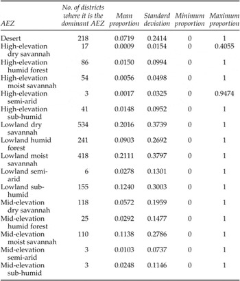
This study develops a completely different approach to measure climate impacts on agricultural revenues using AEZs as the cornerstone of the analysis. One advantage of relying on AEZs is that they are already available for all of Africa. We estimate climate impacts by measuring how climate change alters the distribution of AEZs. An earlier study of Kenya used AEZs to identify starting conditions for farms (Fischer and Van Velthuizen, Reference Fischer and Van Velthuizen1996), but then relied on crop models to predict climate change effects. In this study, we rely on changes of the AEZs themselves to measure climate change effects. AEZs were developed to estimate the underlying agricultural productivity of lands based on their soils and climate (FAO, 1978). The zones were intended to capture the length of the growing season, taking into account soil moisture. The AEZs were based on an assumption that the longer the growing season, the more productive the land would be for crops. The FAO classified every district in Africa using this AEZ methodology and identified the proportion of each AEZ within a district. As shown in table 1, there are a total of 16 AEZs in the continent. Table 1 provides an overview of the frequency of these AEZs. Column 2 indicates the number of districts in which a particular AEZ is dominant (most common). Columns 3–6 provide summary statistics of the contributions of each AEZ to the proportions of the districts we study. Lowland dry savannah and lowland moist savannah are the two most dominant AEZ types in Africa, accounting for 40 per cent of the land. Other common AEZ types include desert, lowland humid forest, lowland sub-humid forest, and mid-elevation dry savannah, which make up an additional 40 per cent of the land.
Current AEZ distribution in Africa

We assume that, ceteris paribus, agricultural productivity is constant within each AEZ. Controlling for market access, we estimate the percentage of land that is cropland and the net revenue per hectare of cropland that is earned in each AEZ. We then analyze how climate affects the allocation of land into each AEZ. We predict how climate change would reallocate land across AEZs. The change in cropland and net revenue per ha is calculated by looking at how the AEZs change over the landscape as climate changes.
There are several assumptions that are required for this analysis to give a representative picture of changes in net returns to agriculture due to climate change in 2070–2100. First, the relationship between AEZs and the fraction of cropland will remain the same. Rising populations may lead to increasing intensification on current cropland as well as expansion of arable land. If the expansion of arable land follows the same pattern as it does currently with respect to AEZs, i.e., the marginal change in the proportion of a district that is cropland with respect to the proportion that is a particular AEZ doesn't change, our analysis suggests that cropland declines in most regions for all climate scenarios. If, however, there is adaptation, our results are an overestimate of the potential impacts.
Second, relative prices and technology are assumed not to change. There have been several previous studies (Reilly et al., Reference Reilly, Hohmann and Kane1994; Adams et al., Reference Adams, Fleming, Chang, McCarl and Rosenzweig1995; Darwin, Reference Darwin2004; Parry et al., Reference Parry, Rosenzweig, Iglesias, Livermore and Fischer2004; Hertel et al., Reference Hertel, Burke and Lobell2010) that found that, once global trade is accounted for, prices of most commodities rise very little or not at all due to climate change for mild to intermediate global warming, although the extent of price impacts depends on the extent of warming and the model assumptions. For more extreme climate change scenarios, this may no longer hold, and prices may rise. If price rises do occur, net seller households in Africa would benefit, leading to increased producer surplus, and net buying households would suffer due to a loss in consumer surplus. If prices do rise, in the case of net selling households, our estimates would overstate the harm to net crop incomes. Regarding technological change and diffusion, it is likely that some adaptation will occur, and trade may increase as climate change occurs, which may mitigate some of the rise in prices. The introduction of new technologies better suited to the new climate would imply that our estimates are a lower bound on the impact on the net crop revenues to agriculture.
Third, since the farm-level data set we rely on for net returns to agriculture is comprised of small-scale and large farms in a manner currently representative of African agriculture, we assume that the current distribution of small and large-scale farms remains constant. If the proportion of large-scale farms in this distribution increases as agriculture is increasingly commercialized, and they are relatively more productive, the actual impacts will be lower than estimated. If the converse occurs due to land fragmentation, they will be higher than estimated.
Overall, we would suggest interpreting our results as the potential changes in cropland and net returns to agriculture – net revenues per ha and overall crop income – if projected climate change were to occur in 2070–2100 and African agriculture in terms of prices, technology and cropping pattern were to remain unchanged. As we mentioned, there are conditions under which this may overstate or understate true damages. However, we consider a careful analysis of the available data, and several of our assumptions are not untenable for mild to moderate climate change. Our results indicate the importance of adaptation to climate change in Africa, as we find that, even under mild climate change, there is a negative impact to crop income of US$ 14–30 billion in 2070–2100. Furthermore, we are able to obtain country-level and regional estimates drawing on the limited data that are currently available, and believe these estimates form an important contribution to the literature on the impacts of climate change.
The underlying AEZ data is composed of the proportions of each AEZ in a district, including some districts that are entirely one AEZ. To take account of both the discrete observations and the proportions in the data set, we use an extension of a generalized linear model (GLM) detailed in Papke and Wooldridge (Reference Papke and Wooldridge1996) (henceforth PW) to estimate the baseline proportions of every AEZ in each of the 2,032 districts in the 48 African countries under consideration.Footnote 1 We also use the GLM model to estimate the baseline proportion of cropland in each district as a function of its AEZ proportions. Baseline net revenue per ha of cropland is estimated using an Ordinary Least Squares (OLS) regression. District-level baseline agricultural revenues are then estimated using each district's net revenue per ha of cropland, and the area as well as proportion of cropland in that district.
We then consider how these AEZ proportions and the proportion of cropland will shift under climate change. For example, climate change may shift a semi-arid AEZ into desert. In theory, changing climates could lead to new types of AEZs being created. However, at least for the next century, it is most likely that land will simply shift from one type of AEZ to another. We assume that a typical farm in a particular AEZ will continue to perform as it does today. As more land leaves one AEZ and shifts to another, both cropland and crop income per ha of cropland will change. Ideally, we would also have liked to measure livestock income per ha and grazing land, but reliable estimates of grazing land are not available in Africa. We use this model to examine the impact of climate change on expected crop net revenue using three very different climate scenarios for 2070–2100.
Section 2 details the methodology and estimation procedure. Section 3 contains an overview of the data. Section 4 presents the empirical results and section 5 describes the results of the climate scenarios. We conclude with the policy implications of the analysis and a summary of the results.
2. Methods
2.1. Theory
We model two crucial decisions made by farmers: a land-use decision to determine the amount of cropland, and a farm management decision to determine net revenue per ha of cropland. We assume that farmers maximize net revenues in both decisions subject to external conditions. Each decision depends on the underlying productivity of the land which is captured by the AEZ, and economic conditions which are captured by market access.
We assume that each parcel of land i could be either cropland or a competing land use. Each land use j generates an associated net present value. We assume that land within districts is heterogeneous and we are not able to observe all relevant site characteristics. The profit πij in choosing to allocate land parcel i to land use j therefore has a random component εj as well as a deterministic component V ij, where V ij is a function of the underlying productivity of the land K i and economic factors s i which include input prices, output prices and interest rates.
 $$\pi _{ij} = V_{ij}\lpar K_{i}\comma \; s_{i}\rpar + \epsilon_{j}\lpar K_{i}\comma \; s_{i}\rpar$$
Defining Z i = (K i, s i), the farmer will choose cropland j over an alternative land use m if:
 $$\pi _{ij}\lpar Z_{i}\rpar \gt \pi _{im}\lpar Z_{i}\rpar \quad \forall m\neq j.$$
When j = cropland, therefore, the probability of choosing cropland is:
 $$P_{ij} = Pr\lsqb \epsilon _{m}\lpar Z_{i}\rpar - \epsilon_{j}\lpar Z_{i}\rpar \lt V_{ij} - V_{im}\rsqb \quad \forall m\neq j \, \hbox{where} \, V_{ij} = V_{ij}\lpar Z_{i}\rpar . \eqno\lpar 1\rpar$$
The second decision by the farmer is to maximize the net revenue of cropland. We assume that the farmer maximizes annual net revenue R i, which is gross revenue minus costs. Gross revenue is output Q i times price P Q and costs are inputs W i times the price of inputs P w. Output is a function of the exogenous crop productivity K i of that parcel and inputs W i. K is used to represent the vector of AEZ-specific productivity profiles.
 $$R_{i} = P_{i}Q_{i}\lpar K_i\comma \; W_i\rpar - P_{W}W_i \eqno\lpar 2\rpar$$
Maximizing (2) with respect to inputs and choosing the crop that yields the highest net revenue leads to a locus of maximum net revenues that are a function of the exogenous variables alone.
 $$R_{i} = F\lpar K_i\comma \; P_{Q}\comma \; P_{W}\rpar \eqno\lpar 3\rpar$$
Equation (3) is the reduced form net revenue regression.
2.2. Empirical approach
The first step in our analysis is to estimate a model that predicts the district-level baseline AEZ proportions as a function of climate, elevation and latitude. Note that this equation is not a farmer's choice model but rather is a prediction of what determines AEZs. It is a description of the ecological production function. The purpose of the AEZ methodology is to classify agricultural productivity by AEZs (K) as well as by economic variables (P Q, P X), which we capture using market access variables. We use household-level survey data measuring net revenue per ha from 11 African countries to estimate net revenue effects and remote sensing cropland data and AEZ classifications for all of Africa to estimate cropland effects.
The AEZ data and the data on the proportion of land in cropland contain both zeroes and ones as well as proportions. There are several methods to estimate a dependent variable that is a proportion (Cox and Wermuth, Reference Cox and Wermuth1996; PW, Reference Papke and Wooldridge1996; Kieschnick and McCullough, Reference Kieschnick and McCullough2003; Ospina and Ferrari, Reference Ospina and Ferrari2010). These include parametric approaches – for instance, using the log-odds transformation or assuming that the dependent variable under consideration has a beta distribution, as well as semi-parametric methods such as the fractional logit approach using quasi-likelihood estimation (PW, Reference Papke and Wooldridge1996). The log-odds transformation requires arbitrary conversions to accommodate values that are zero or one, whereas the beta distribution assigns a probability of zero to {0, 1}, and hence may also be problematic to apply to data sets that have a non-trivial proportion of boundary values. While we could assume an inflated beta distribution (Ospina and Ferrari, Reference Ospina and Ferrari2010) which could accommodate boundary values, this includes the condition that the process by which the boundary values are generated are structurally different from the non-boundary values, a condition which does not hold in our data.
Since the 16 AEZs encompass all the possible states of nature, the sum of the AEZ proportions in a district should add up to one. This is assured in a multivariate logit regression of a linear combination of the independent variables (Aitchinson, Reference Aitchison2003) or with the Dirichlet distribution, which is a multivariate generalization of the beta distribution. Unfortunately, these techniques require making several assumptions for the variance-covariance structures of the dependent variables. Since we are interested in predicting mean AEZ proportions and not the full distributions of the AEZ proportions, we can avoid making these assumptions by relying on a generalization of the PW semi-parametric method.
In order to estimate the proportion of each of the 16 AEZs in the 2,032 districts, we use a GLM with a binomial link function to estimate a proportional dependent variable. GLM models provide a flexible approach to estimate the mean of a dependent variable by assuming a link function that determines the relationship between the dependent variable and the linear index of independent variables. An OLS regression provides the simplest case of a GLM with the identity function as the link function. The resulting estimator is consistent and  $\sqrt{N}$ asymptotically normal. The GLM with binomial link function was outlined in McCullagh and Nelder (Reference McCullagh and Nelder1989). PW use the GLM framework as a general approach to estimate the mean of proportional dependent variables, consider the logit link function in particular, and provide robust variance estimators as well as goodness of fit estimates for this specification. This model is capable of dealing with {0,1} values as well as proportions. Extending the PW approach for multivariate estimation thus provides a flexible and tractable estimation method, incorporates boundary values (0 and 1), and only requires that the link function be correctly specified. This estimation strategy leads to predicted values that lie between zero and one, and which sum to 1. It also fulfills the requirements for quasi-likelihood estimation, since our link function, the multinomial logit, is a member of the linear exponential family (LEF).
PW lay out a general framework for using a GLM to estimate a univariate dependent variable y that is a proportion as a function of explanatory variables X, specifically using the logit link function:
 $$E\lpar y\vert X\rpar = G\lpar X\beta\rpar$$
where β is the vector of regression coefficients and 0 < G(Xβ) < 1 is strictly increasing and is usually, though not necessarily, a cumulative distribution function. With the logit link function, we obtain
 $$E\lpar y\vert X\rpar = G\lpar X\beta\rpar = {\displaystyle{\exp \lpar X\beta \rpar }\over{1 + \exp \lpar X\beta \rpar }}.$$
The Bernoulli log likelihood function used in PW is given by
 $$l_{i} = y_{i}\ln \lsqb G\lpar x_{i}\beta \rpar \rsqb + \lpar 1 - y_{i}\rpar \ln \lsqb 1 - G\lpar x_{i}\beta \rpar \rsqb . \eqno\lpar 4\rpar$$
Since the logit function is a member of the LEF, the quasi-maximum likelihood estimator (QMLE) of β is consistent and asymptotically normal, irrespective of the actual distribution of y conditional on X.
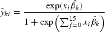
We extend the binomial GLM in PW with the multinomial logit as a link function to estimate the different AEZ proportions. This ensures that each of the predicted AEZ proportions for a given district lie in the unit interval and the sum of the predicted AEZ proportions for each district equal 1. The predicted proportion ŷ ki of AEZ k for district i is thus given by
 $$\hat{y}_{ki} = {\displaystyle{\exp \lpar x_{i}\hat{\beta _{k}}\rpar }\over{1 + \exp \left(\sum_{j=0}^{15}x_{i}\hat{\beta}_{k}\right)}} \eqno\lpar 5\rpar$$
where βk is a vector of coefficients for AEZ k and x i is a vector of seasonal temperature and precipitation variables, elevation and latitude. Since the multinomial logit link function is a member of the LEF, we can follow the PW approach and apply the quasi-likelihood maximization procedure.
We generalize (4) and use a multinomial log-likelihood function, L(X, y, β). For district i:
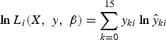 $$\ln L_{i}\lpar X\comma \; y\comma \; \beta \rpar = \sum_{k=0}^{15}y_{ki}\ln \hat{y}_{ki} \eqno\lpar 6\rpar$$
where the expression for ŷ ki is given by (5). The quasi-likelihood estimator  $\hat{\beta}$ is thus the solution to
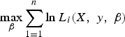 $$\max_{\beta }\sum_{1=1}^{n}\ln L_{i}\lpar X\comma \; y\comma \; \beta\rpar$$
which is consistent and asymptotically normal.Footnote 2 The standard errors reported are robust to heteroskedasticity.
We estimate the proportion of cropland in each district, as a function of observed AEZ proportions in each district. We use the binomial GLM model to estimate the proportion of cropland. Note that the proportion of cropland is a logit analysis and uses the binomial function as a link function in the GLM. Thus, equation (5) is the predicted mean cropland proportion and (6) the corresponding log-likelihood:
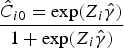 $$\hat{C}_{i0} = \displaystyle{\exp \lpar Z_{i}\hat{\gamma}\rpar }\over{1 + \exp \lpar Z_{i}\hat{\gamma}\rpar }$$
where Z is are the AEZ proportions in the ith district, Ĉ i0 is the baseline predicted fraction of cropland in the ith district and γ is the vector of coefficients.
The log-likelihood function is given by
 $$L_{i}\lpar Z_{i}\comma \; C_{i}\comma \; \gamma \rpar = \lsqb C_{i}\ast \ln F\lpar Z\hat{\gamma}\rpar \rsqb + \lsqb \lpar 1-C_{i}\rpar \ast\lcub \ln \lpar 1 - F\lpar Z\hat{\gamma}\rpar \rpar \rcub \rsqb .$$
Thus, the vector of estimators,  $\hat{\gamma}$, is consistent and is given by the solution to
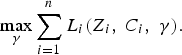 $$\max_{\gamma }\sum_{i=1}^{n}L_{i}\lpar Z_{i}\comma \; C_{i}\comma \; \gamma\rpar .$$
In addition to the AEZ proportions, we include the annual mean flow of water in each district as an explanatory variable to measure potential water availability for irrigation. This is an exogenous measure of potential water availability and does not reflect any decisions by farmers. However, it likely influences whether or not cropland is chosen. As suggested in (1), we also include the influence of market prices. Because this is a cross-sectional analysis, we assume that the underlying global market prices are constant. We assume that all the variation in local market prices is due to differential market access such as the distance to the nearest port and the distance to the nearest major city.
Finally, we estimate the net revenue per ha of cropland R i, using an OLS regression, where the net revenue data is taken from 395 districts in the 11 countries where the household survey was conducted. The AEZ proportions y ik, annual mean flow f i, and market access variables m i are the independent variables. We use the natural log of R i as the dependent variable:
 $$\ln R_{i} = \beta_{y}\hat y_{ik} + \beta_{f}f_i + \beta_{m}m_i+\mu\comma \; \ k=1\comma \; 2\comma \; \ldots 16.$$
Because we are interested in predicting the value of net revenue from the predicted values of ln(net revenue), we include a correction term αi for the log transformation that uses the standard error of the predicted value σ (Goldberger, Reference Goldberger1968; Kennedy, Reference Kennedy1983):
 $$\alpha_{i} = \lpar \sigma^{2}/2\rpar \Rightarrow \hat{R}_{I} = \exp \lpar Z\hat{\beta} + w_{i}\rpar .$$
We then use the coefficients of the OLS regression above to calculate the predicted net revenue values of all 2,032 districts. This is the baseline predicted net revenue per ha in a district, and is a function of the proportion of each AEZ, the mean flow and market access in that district.
3. Data
Data on net returns to agriculture were obtained from a 2002–2004 household-level survey conducted in 11 African countriesFootnote 3 as part of a collaborative project undertaken by several institutions and country partners. There is a great deal of climate variation across the continent, and the districts within the 11 countries were chosen to be representative of ‘all key agroclimatic zones and farming systems in Africa’ (Dinar et al., Reference Dinar, Hassan, Mendelsohn and Benhin2008). Since the data is representative of the current farming systems, including the composition of small-scale and commercial farms, we take the mean of the net revenue at the district level as our measure of district-level crop income. Within each country, 30–50 districts were selected to capture representative farms across diverse agroclimatic conditions.Footnote 4 Sampling was clustered in villages, with villages randomly selected within chosen districts. In each selected village, surveys were conducted in 2002–2004 of randomly selected farms (seven countries were surveyed in the 2002–2003 season and four countries were added in 2003–2004). A total of 9,597 surveys were administered. The final number of surveys with usable information on crop production was 9,064. Of these, 7,238 farms had dryland crops and 1,221 had irrigated crops. The total number of farm surveys per country varied from 222 in South Africa to 1,288 in Burkina Faso. The relative importance of rainfed and irrigated crops varies considerably. For instance, Egypt is entirely dependent on irrigated crops because the climate is too dry to support crops without irrigation. In contrast, most farms in East Africa and the Sahel have very little irrigated agriculture.
Data on climate was gathered from two sources. Temperature data came from polar orbiting satellites operated by the Department of Defense (Basist et al., Reference Basist, Grody, Peterson and Williams1998). The precipitation data came from interpolations between weather stations made by the National Oceanic and Atmospheric Association's Climate Prediction Center – Africa Rainfall and Temperature Evaluation System (ARTES) (World Bank, 2003), which has been used for several previous studies on climate change impacts (Kurukulasuriya et al., Reference Kurukulasuriya and Mendelsohn2006; Kurukulasuriya and Mendelsohn, Reference Kurukulasuriya and Mendelsohn2008). We defined the seasons in the northern hemisphere as the average of November, December and January for winter, the next three months as spring, the three months after that as summer, and August, September and October as fall. We then adjusted for the fact that seasons in the southern and northern hemispheres occur at exactly the opposite months of the year – so the average of November, December and January would be defined as summer in the southern hemisphere. While this causes a discontinuity in the definition of seasons near the equator, in practice, the climate in all four seasons around the equator is very similar, particularly temperature. Thus, the measurement error due to the way that seasons are defined above and below the equator is likely to be quite small.
AEZs were classified by FAO (1978). Data on elevation at the centroid of each district were obtained from the United States Geological Survey (USGS, 2004), which was derived from a global digital elevation model with a horizontal grid spacing of 30 arc seconds (approximately 1 km). The University of Colorado and the International Water Management Institute (IWMI) estimated mean flow (which indicates the amount of water entering a district from higher elevation) for all the districts under consideration (IWMI/University of Colorado, 2003). Data on market access variables were obtained from the World Bank. These comprised the travel time in hours to the nearest port and the travel time in hours to the nearest major city,Footnote 5 based on extant road networks. Both are measured from the centroid of each district.
Data on the fraction of cropland at the 1 km2 scale for each district in Africa were obtained from several sources and vary widely. These differences are partially attributable to lack of consistent definitions of the categories of land useFootnote 6 and differences in measurement techniques and technologies (Lotsch, Reference Lotsch2007). This is true more generally of global land-use models. For instance, Giri et al. (Reference Giri, Zhu and Reed2005) compare two widely used global land-use models and find large differences between them for disaggregated land classes, with the extent of the discrepancies varying across biomes. Thus, there is considerable variation in definitions of what constitutes cropland, particularly for Central Africa where forest cover makes satellite data from different sources inconsistent. Cropland measures using satellite data are vulnerable to these errors, and so we rely on two widely used estimates of cropland, from the International Food Policy Research Institute (IFPRI) and the University of Maryland (UMD). The total amount of cropland in Africa is 322 million ha according to the IFPRI estimate and 132 million ha according to the UMD estimate. It is important to recognize that these two estimates of cropland are quite different, given that they refer to the exact same land base. While both the measures of cropland are widely recognized and used, we would tend to rely more on the IFPRI estimates since they were more thoroughly corroborated with secondary estimates of ground-level cropland estimates. Data on latitude was obtained from ARC-GIS software.
4. Empirical Results
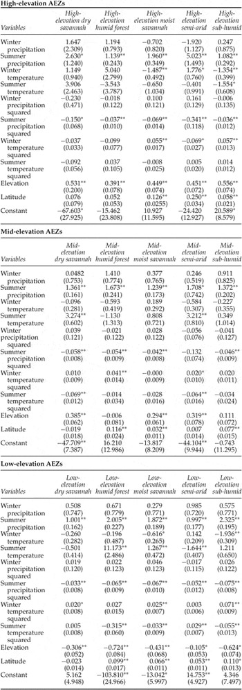
This section presents and discusses the results of the empirical model. Table 2 presents the results of the fractional multinomial logit used to predict the proportions of each AEZ in each district. The table is organized by high-, mid- and low-elevation AEZs. The omitted AEZ is the desert. Summer precipitation and summer precipitation squared are statistically significant for predicting AEZ proportions for nearly all the AEZs. Winter precipitation and winter precipitation squared are generally not significant. Winter temperature is statistically significant for predicting the proportion of high-elevation AEZs in particular, and summer temperature for predicting low-elevation AEZs. As is expected from the definitions of AEZs, elevation is also important.
Fractional multinomial logit of AEZ proportions
Log pseudo-likelihood = −1,738.6587 2(150) = 4,087.02
Mac Fadden's adjusted pseudo-R 2 = 0.62 Prob > chi2 = 0.0000
Nagelkerke/Cragg & Uhler's pseudo-R 2 = 0.99
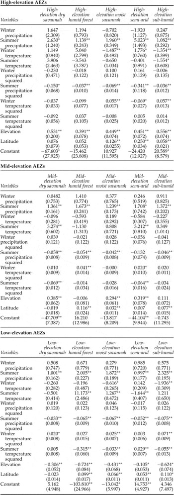
Notes: There are 2,032 observations. The omitted AEZ is desert. Robust standard errors in parentheses. **p < 0.01, *p < 0.05.
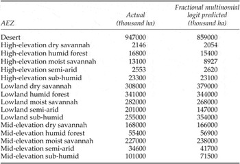
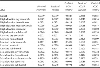
Table 3 provides the actual amount of land under each AEZ as well as the amount of land predicted by the fractional multinomial logit in each AEZ. The model predicts land under particular AEZs quite well, especially for high- and mid-elevation AEZs. However, area under desert, lowland sub-humid and mid-elevation sub-humid AEZs is not as reliably predicted.
Actual and fractional multinomial logit-predicted land under AEZs

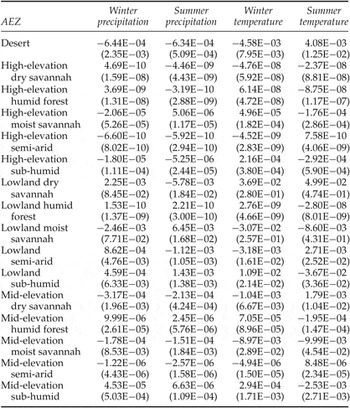
Table 4 presents the marginal climate results for the AEZ fractional multinomial logit. As expected, as summer precipitation increases, the proportion of land in deserts and dry savannah falls and the proportion of land in forests and moist savannahs generally increases. A one degree rise in summer temperature increases the predicted proportion of AEZs in desert and reduces the proportion of land in moist savannah at all elevations. But, as winter temperature rises, there is a small reduction in desert and semi-arid AEZs with a corresponding increase in forest at all elevations and moist savannah at high-elevation.
Marginal climate effects on AEZ proportions

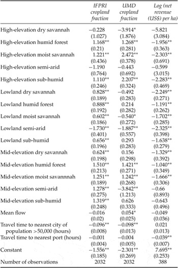
Table 5 presents the fractional logit results of the cropland model for both cropland measures. The independent variables include (actual) proportions of AEZs (with desert as the omitted AEZ), mean flow, travel time in hours to the nearest city with population greater than 50,000 people, and travel time in hours to the nearest port. The coefficients on proximity to the nearest city have the expected negative signs – the fraction of cropland falls as markets become less accessible. However, proximity to ports is not significant. Districts with greater mean water flow (more surface water) have more cropland using the UMD cropland measure. However, flow is not significant when the IFPRI measure of cropland is used.
Fractional logit results of cropland fraction and OLS of net revenue per hectare

Notes: Robust standard errors in parentheses. **p < 0.01, *p < 0.05
Examining the coefficients of the AEZ proportions, three AEZs – high- and low-elevation semi-arid and high-elevation dry savannah – have less cropland than desert. With the UMD cropland measure, mid-elevation semi-arid and low-elevation moist savannah have less cropland than desert as well. The remaining AEZs have more cropland than deserts. With the UMD cropland measure, high-elevation moist savannah, high-elevation sub-humid forest, and mid-elevation humid forests have the most cropland. With the IFPRI cropland measure, only mid-elevation humid forests have particularly high proportions of cropland.
Table 5 also presents the OLS regression results of logged net revenues per ha. The desert is the omitted AEZ category. Interestingly, the distance to nearest city was not significant nor was it negative. The fraction of land in cropland is higher near cities but the net revenue per ha is not. The coefficient for mean flow was also not statistically significant. The coefficient on the travel time to the nearest port is significant and negative, implying that greater proximity to a port increases net returns. A possible explanation for why the travel time to ports has a statistically significant role in explaining net revenues but not cropland is that proximity to ports affects prices positively. However, the acreage available is determined largely by geophysical variables such as climate and soils and not economic forces (inelastic supply). In contrast, net revenues per ha may be much more sensitive to prices (price elastic response) both in terms of inputs and outputs. The AEZ with the highest valued cropland is the desert. This is probably because the cropland in the desert is irrigated whereas most of the cropland in Africa is rain fed. We tested this assumption using data on irrigation status in our household-level data set, and found that the marginal effect on the probability of irrigation is highest as the proportion of desert in a district increases, relative to any other AEZ.Footnote 7 Looking across the rest of the AEZs, the next most valuable cropland was in high-elevation semi-arid, mid-elevation semi-arid, and mid-elevation sub-humid forest AEZs. The lowest valued cropland was in high-elevation dry savannah.
5. Climate Simulations
The total baseline (current) cropland net revenue of district i, T i0 is defined as:
 $$T_{i0} = A_{i}\ast C_{i0}\lpar y_{0}\rpar \ast R_{i0}\lpar y_{0}\rpar$$
where A i is the area of the district i, C i0 is the baseline proportion of cropland and R i0 is the baseline mean net revenue per ha of cropland in a given district. T i0 is dependent on the initial proportions of AEZs (y i0), the observed flow and the current market access.
With climate change, the new cropland income T i1 is dependent on the change in the AEZs for each district. As the proportion of AEZs y ik changes, both the proportion of cropland, C, and the net revenue per ha, R, will change:
 $$T_{i1} = A_{i}\ast C_{i1}\lpar y_{1}\rpar \ast R_{i1}\lpar y_{i1}\rpar .$$
We assume that the welfare effect of climate change on cropland is the change in crop net revenue (∑i=1nY i1 – ∑i=1nY i0). To the extent that aggregate cropland changes, it is not a complete welfare measure. The measure assumes a zero opportunity cost of land not used for crops and in that way overestimates the overall welfare effect. A reduction (increase) in cropland leads to an increase (decrease) in land for other uses so the true future welfare impact is higher (lower).
We use climate predictions for 2070–2100 from three different climate models: the Parallel Climate Model (PCM; Washington et al., Reference Washington, Weatherly, Meehl, Semtner, Bettge, Craig, Strand, Arblaster, Wayland, James and Zhang2000), the Centre for Climate System Research (CCSR; Emori et al., Reference Emori, Nozawa, Abe-Ouchi, Namaguti and Kimoto1999), and the Canadian Climate Centre (CCC; Boer et al., Reference Boer, Flato and Ramsden2000) models. These predictions were chosen because they span the range of likely outcomes predicted by the Fourth Assessment Report (IPCC, 2007a). We use the predicted absolute change in temperature and the percentage change in precipitation from the 2000–2010 decade to 2070–2100 from each climate model. The PCM model suggests mild temperature increases of about 2°C and small gains in precipitation in both the summer and winter months. The CCC model suggests considerable warming in 2070–2100 of over 5°C with dryer summers and wetter winters. The predictions of the CCSR lie between those of the PCM and the CCC models. In addition, there is some variation in how climate is expected to change across the continent. District changes in temperature are calculated by adding the predicted country temperature changes to the observed district temperature. Precipitation changes are calculated by multiplying predicted percentage changes in precipitation by the observed district rainfall values.
We use the coefficients from table 2 to predict the AEZ proportions of each district under current climate conditions and for each climate change scenario. Table 6 illustrates how climate change alters the AEZ proportions in 2070–2100. It presents the actual and FML-predicted baseline means of the AEZ proportions for comparison. Note that the fractional multinomial logit predicts the mean baseline AEZ proportions quite well. The key results in table 6, however, concern the predicted changes in the mean AEZ proportions under each of the three climate scenarios. Climate change increases the mean proportions of high-, mid- and low-elevation dry savannah and decreases the mean proportions of high-, mid- and low-elevation humid forest. The magnitude of the change is proportional to the magnitude of the underlying climate change. Interestingly, the amount of desert does not systematically increase with warming. It appears that the amount of desert is much more sensitive to changes in precipitation than changes in temperature. With rising precipitation, the amount of desert falls in the hottest scenario.
Mean predicted AEZ proportions – baseline and in 2070–2100

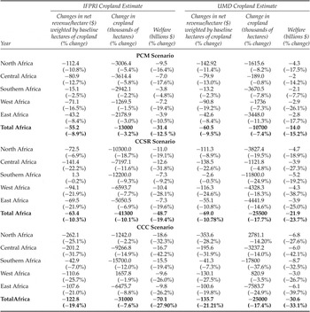
Armed with the changes in AEZs, coefficients from the first two columns of table 5 are used to examine the changes in cropland fractions. Similarly, the coefficients from the third column of table 5 are used to calculate mean district net revenue per ha of cropland. The climate change effects are the differences between the baseline and the new climate scenario outcomes. Table 7 presents the absolute and percentage changes in net revenue, cropland and welfare for each climate scenario for 2070–2100 for all of Africa and for each region.Footnote 8 There are separate estimates for the IFPRI and the UMD measures of cropland. The climate scenarios predict that cropland will generally shrink for Africa as a whole.
Projected changes in net revenue per hectare, cropland and crop income for 2070–2100

In 2070–2100, the mild PCM prediction leads to a reduction of 13 and 10 million ha with the IFPRI and UMD cropland measures, respectively. The worst cropland scenario is with the dry CCSR model. The CCSR model predicts that cropland will shrink by 41 and 25 million ha with the IFPRI and UMD cropland measures respectively. Under the very warm but wet CCC scenario, the IFPRI cropland measure falls by 31 million ha and the UMD cropland measure falls by 25 million ha. The IFPRI cropland measure is more sensitive to warming than the UMD cropland measure. Net revenue per ha is also predicted to fall by 2100 as climate changes. The more severe the increase in temperature, the larger the loss in net revenue per ha. Using the IFPRI cropland measure, the projected losses are US$ 55/ha, US$ 63/ha and US$ 123/ha under the PCM, CCSR and CCC climate scenarios, respectively. Using the UMD estimate, they are US$ 61/ha, US$ 69/ha and US$ 136/ha, respectively. Combining the change in cropland and the change in net revenue, the expected welfare impacts of climate change under all three climate scenarios are negative. Using the IFPRI cropland measure, the annual projected losses of aggregate net revenues are US$ 31 billion (12.5 per cent), US$ 49 billion (19.4 per cent) and US$ 70 billion (27.9 per cent) in the PCM, CCSR and CCC climate scenarios, respectively. Using the UMD cropland measure, the annual projected welfare losses are US$ 14 billion, US$ 22 billion and US$ 31 billion, respectively. The more severe the temperature increase in the climate scenario, the larger are the agricultural losses in Africa. The IFPRI cropland measure leads to slightly higher welfare losses than the UMD cropland measure.
Every region in Africa suffers annual welfare losses in every climate scenario. However, the magnitude of the losses varies across regions. As expected, Southern Africa, which is cooler, generally has the smallest aggregate net revenue losses of all the regions. West Africa suffers the largest aggregate net revenue losses in the PCM scenario, Central and West Africa have the largest losses in the CCSR scenario, and Central Africa has the largest losses in the CCC scenario. The relatively harsh welfare outcomes for Central and West Africa are due to large reductions in net revenue per ha in those regions. These effects are driven more by temperature than precipitation. The regional effects of climate on cropland depend on the cropland measure and the climate scenario. With the IFPRI cropland measure, West Africa and East Africa often have the smallest cropland losses (with a gain in the CCC scenario). With the UMD cropland measure, Central Africa and North Africa have the smallest losses (with a gain in the CCC scenario for North Africa). With the IFPRI cropland measure, Central Africa and North Africa have the largest cropland losses. With the UMD cropland measure, West Africa and Southern Africa have the largest cropland losses. It is not clear why the two cropland measures give such different regional cropland predictions.
The figures in the online appendix (available at http://journals.cambridge.org/EDE) provide maps showing district-level welfare impacts for all three scenarios using the IFPRI cropland measure. The maps for the UMD cropland measure look very similar to the maps shown. Overall, the welfare impacts vary widely across the continent. The mild PCM scenario results in relatively uniform and mild impacts across Africa. The CCC scenario shows more heterogeneous impacts across space. There are also consistent results in different locations. There is a band of districts in the Sahel that are quite sensitive to warming. This band expands as one moves from the PCM to CCC climate scenarios. There are also scattered locations along the Mediterranean that may benefit from warming.
6. Conclusion
This study is based on a concept first introduced by the FAO that a complex landscape could be represented as a set of homogenous production zones, AEZs. We rely on this insight to develop an alternative method to evaluate climate change impacts. For each AEZ, we estimate the net revenue per ha and cropland associated with that zone. We also predict how temperature and precipitation influence the proportion of each AEZ. The impact of climate change on agriculture is measured by the change in the proportion of each AEZ in each district. Temperature and precipitation forecasts from climate models are used to predict how AEZs will shift in each district in Africa. Warming generally causes AEZs to shift from more productive categories to less productive categories. The analysis measures the resulting damages. These changes in AEZs in turn lead to changes in both cropland and net revenue per ha of cropland. Combining these two effects leads to an estimated total change in crop net revenue. Estimates of cropland in Africa vary a great deal across measures and so two separate calculations of impacts are made for the IFPRI and the UMD measure of African cropland.
Climate change shifts the AEZs towards desert and semi-arid classifications. This generally leads to a reduction in cropland. With the IFPRI measure of cropland, climate change impacts reduce aggregate cropland in Africa by 13 million ha (−3 per cent) with the mild PCM climate scenario and by 41 million ha (−10 per cent) with the dry CCSR climate scenario. With the UMD measure of cropland, cropland falls by 11 million ha (−7 per cent) with the PCM climate scenario and by 26 million (−18 per cent) with the CCSR climate scenario.
The shifts in AEZs also cause a change in net revenue per ha. This change is more closely associated with the temperature change than the change in precipitation. With the IFPRI cropland measure, the change in net revenue per ha ranges from a loss of US$ 55/ha under the PCM scenario to a loss of US$ 123/ha under the CCC scenario. With the UMD cropland measure, the net revenue per ha losses range from US$ 61/ha to US$ 136/ha under the PCM and CCC climate scenarios, respectively.
Overall annual welfare losses are calculated by combining the change in cropland with the change in net revenue per ha. The annual losses range from US$ 31 billion to US$ 70 billion with the IFPRI cropland measure and from US$ 14 to US$ 31 billion with the UMD cropland measure. The losses get steadily larger as the climate scenario becomes more severe, moving from the PCM to the CCSR to the CCC climate scenarios.
The welfare effects are negative in every African region but the magnitude of the effects varies regionally. The percentage welfare losses are smallest in Southern Africa and largest in West Africa and Central Africa, depending on the scenario. The regional changes in welfare tend to mirror the regional net revenue per ha changes. However, the changes in cropland have different patterns. West and Central Africa have the smallest losses (and sometimes gains) in cropland, whereas Central Africa and Southern Africa have the largest cropland effects. These regional cropland effects are almost in opposite directions for the IFPRI and UMD cropland measures. The Central African results are perhaps the least reliable, possibly because the rainfall in that region leads to substantial forest cover, making satellite measures of cropland difficult.
The paper shows that measuring how climate change shifts AEZs leads to a viable measure of agricultural impacts. The results rely on limited data and are consistent with other African results from agronomic studies (Rosenzweig and Parry, Reference Rosenzweig and Parry1994; Parry et al., Reference Parry, Rosenzweig, Iglesias, Livermore and Fischer2004) and Ricardian studies (Kurukulasuriya et al., Reference Kurukulasuriya and Mendelsohn2006; Kurukulasuriya and Mendelsohn, Reference Kurukulasuriya and Mendelsohn2008). The magnitude of the impacts is similar and the sensitivity to different climate scenarios is similar.
The strength of the shifting AEZ approach is that it provides comprehensive measures of impacts across the landscape and it is relatively easy to implement. In addition, the knowledge of which AEZs become more likely under different climate scenarios and how that affects the pattern of cropland and crop incomes across Africa provides insights into possible adaptation measures such as irrigation, and is thus very policy-relevant.
However, there are also weaknesses in this new approach. As with the Ricardian and agronomic techniques, the AEZ model cannot capture the change in relative prices caused by climate change. Our results indicate that African agricultural production falls due to climate change. If this fall in production causes prices to rise, our estimates overestimate the welfare damage of climate change. While this is a weakness of the study, current literature indicates that, with international trade, global food supply and global food prices are not likely to change drastically with moderate climate change. Thus, it is plausible that the overestimate of losses to crop income is not likely to be very large. Another potential weakness of the AEZ approach is that the AEZ classifications may not capture all aspects of natural productivity. Thirdly, good measures of economic factors are not easily attainable in Africa. The absence of available data meant that we could not extend the approach to livestock. Carbon fertilization effects were not included. Finally, changes in the baseline that occur over time such as new technology (machinery, varieties, fertilizers, insecticides) could not be factored into the analysis. There is clearly room to improve the AEZ methodology and other methods with better data. These and related questions pose interesting and relevant issues for future research.
Appendix A: Countries by region
(1) North – Algeria, Egypt, Libya, Mauritania, Morocco, Sudan, Tunisia
(2) South – Angola, Botswana, Lesotho, Madagascar, Malawi, Mozambique, Namibia, South Africa, Swaziland, Zambia, Zimbabwe
(3) East – Burundi, Djibouti, Eritrea, Ethiopia, Kenya, Rwanda, Somalia, Tanzania, Uganda
(4) West – Benin, Burkina Faso, Chad, Cote d'Ivoire, Equatorial Guinea, Gambia, Ghana, Guinea, Guinea-Bissau, Liberia, Mali, Nigeria, Niger, Senegal, Togo, Central Cameroon, Central African Republic, Democratic Republic of Congo, Gabon, Republic of Congo, Sierra Leone