Nomenclature
-
 ${[}{A}_{\mathcal{M}}^{1}{]},{[}{A}_{\mathcal{M}}^{2}{]}$
-
aerodynamic mass matrices
-
${[}{A}_{\mathcal{Q}\mathcal{S}}^{1}{]},{[}{A}_{\mathcal{Q}\mathcal{S}}^{2}{]}$
-
aerodynamic quasi-steady matrices
-
${[}{A}_{\mathcal{W}}^{1}{]},{[}{A}_{\mathcal{W}}^{2}{]}$
-
aerodynamic wake matrices
-
$b$
-
half chord length
-
$C$
-
chord length
-
$C(k)$
-
Theodorsen’s function
-
${C}_{L},\text{}{C}_{M}$
-
steady lift and moment coefficients, respectively
-
$\overline{{C}_{L}},\overline{{C}_{M}}$
-
amplitudes of the unsteady lift and moment coefficients, respectively
-
${C}_{T}$
-
membrane tension coefficient =
$=T/({q}_{\infty }c)$
-
$\mathbb{D}$
-
dimension of the PCE
-
$E$
-
elastic modulus
-
$E{[\,\,]}$
-
probabilistic mean operator
-
$e$
-
exponential function
-
$\mathcal{F}$
-
basis function of the PCE
-
$\left\{{f}_{\mathcal{Q}\mathcal{S}}\right\},\left\{{f}_{\mathcal{W}}\right\},\left\{{f}_\mathcal{M}\right\}$
-
nodal aerodynamic force vectors due to quasi-steady, wake, mass and gust,
-
$\text{and}\ \{\vec{f}_{g}\}$
-
respectively
-
$h$
-
membrane thickness
-
${H}_{0}^{\left(2\right)},{H}_{1}^{\left(2\right)}$
-
Hankel functions of the second kind of the zeroth and first orders, respectively
-
${\mathbb H}_{n}$
-
basis function of the KLE of order
$\left(n\right)$
-
$\mathbb{K}$
-
correlation function of the KLE
-
$k$
-
reduced frequency of the membrane motion =
$\omega b/{V}_{\infty}$
-
${k}_{LE}$
,
${k}_{TE}$
-
stiffness coefficients of the leading edge and trailing edge springs
-
${[}{K}_{u}{]},{[}{K}_{w}{]}$
-
in-plane and out-of-plane FE stiffness matrices, respectively
-
${\unicode{x1D55D}}_{c}$
-
correlation length of the KLE series
-
${l}_{e}$
-
length of a finite element
-
${[}M{]}$
-
FE mass matrix
-
${n}_{s}$
-
number of structural elements
-
$N$
-
number of terms in the KLE series
-
$\lfloor{N}_{s}\rfloor$
-
FE shape function
-
${[}{N}_{uw}^{\left(2\right)}{]}={{[}{N}_{wu}^{\left(2\right)}{]}}^{T}$
-
in-plane and out-of-plane coupling nonlinear FE stiffness matrix
-
${[}{N}_{ww}^{\left(2\right)}{]},{[}{N}_{ww}^{\left(3\right)}{]}$
-
second-order and third-order nonlinear FE out-of-plane stiffness matrices
-
$\mathbb{O}$
-
order of the PCE series
-
${\mathcal{P}^{qs}},{\mathcal{P}^m},{\mathcal{P}^w}$
-
aerodynamic quasi-steady, mass, and wake pressure terms, respectively
-
${q}_{\infty }$
-
free stream dynamic pressure
-
$\left\{{\vec{q}}_{u}\right\}$
-
in-plane FE membrane deformation vector
-
$\left\{{\vec{q}}_{w}\right\}$
-
out-of-plane FE membrane deformation vector
-
$\Re $
-
stiffness ratio between the LE spring to the TE spring
-
$s$
-
nondimensional coordinate of a finite element
-
$S\left({k}_{g}\right)$
-
Sears’ function
-
${\mathbb{S}}_{{{\Theta}}_{i}}^{\left(1\right)},{\mathbb{S}}_{{{\Theta}}_{i}}^{\left(T\right)}$
-
first-order and total sensitivity measures, respectively
-
$t$
-
time
-
${t}^{*}$
-
nondimensional time =
$t{V}_{\infty }/b$
-
$T$
-
membrane tension force
-
$\mathcal{T}$
-
kinetic energy
-
$u$
-
membrane in-plane deformation
-
$U$
-
strain energy
-
${V}_{\infty }$
-
free stream speed
-
$Var{[}{]}$
-
probabilistic variance operator
-
$w$
-
membrane out-of-plane deformation
-
${w}_{g}$
-
free stream gust speed
-
${W}_{g}$
-
amplitude of a sinusoidal gust speed
-
$W$
-
external work
-
$x$
-
membrane chord-wise coordinate measured from the mid-chord
-
${x}^{*}$
-
membrane chord-wise nondimensional coordinate =
$x/b$
-
$Z$
-
Standard normal random variable


Greek symbols
-
$\alpha $
-
free stream angle-of-attack
-
$\delta $
-
variational operator
-
${\varepsilon }_{x}$
-
membrane strain
-
$\eta $
-
nondimensional coordinate of a finite element
-
${\Theta}$
-
input random variable
-
$\lambda $
-
eigenvalue of the correlation function in the KLE
-
${\Lambda }$
-
aerodynamic inertia function
-
$\mu $
-
probabilistic mean
-
$\xi $
-
membrane chord-wise coordinate measured from the mid-chord
-
${\xi }^{*}$
-
membrane chord-wise nondimensional coordinate =
$\xi /b$
-
$\pi $
-
Pi constant
-
${\rho }_{\infty }$
-
free stream air density
-
$\varrho $
-
membrane density per unit length
-
$\sigma $
-
probabilistic standard deviation
-
$\tau $
-
time
-
${\Upsilon }$
-
output random variable
-
$\varphi $
-
aerodynamic Wagner’s function
-
$\psi $
-
eigenfunction (Basis functions) of the KLE
-
$\omega $
-
frequency of the membrane motion
-
${\omega }_{g}$
-
frequency of the free stream gust
- Ω
-
frequency parameter in the basis functions of the KLE


Abbreviations
-
probability density function
- PCE
-
polynomial chaos expansion
- KLE
-
Karhunen-Loéve Expansion
- FE
-
finite element
- LE
-
leading edge
- TE
-
trailing edge
- CoV
-
coefficient of variation =
$\sigma /\mu $

Superscripts
-
${\left(\,\right)}^{e}\text{}$
-
refers to an elemental constant, vector, or matrix

1.0 Introduction
Aeroelastic analysis of an aerospace structure is a multidisciplinary analysis that requires studying the interactions between aerodynamic loading, a structure’s elasticity and inertial loads. The aeroelastic design of an aerial vehicle is usually done assuming deterministic design parameters and loading scenarios, but in reality, these parameters might deviate from the design values, which would affect the vehicle’s performance. These deviations can be represented probabilistically using probability density functions (PDFs), and in this case, the analysis is known as aleatoric (stochastic) aeroelastic uncertainty analysis. On the other hand, if these deviations cannot be quantified, or if the exact mathematical model representing a physical phenomenon is not known, then the analysis is known as epistemic aeroelastic uncertainty analysis. Over the past years, the study of different kinds of uncertainties in aeroelasticity has gained the interest of researchers and engineers [Reference Beran, Stanford and Schrock1–Reference Bijl, Lucor, Mishra and Schwab3]. This paper considers the uncertain aeroelastic analysis of membrane aerofoils. Therefore, in this section, a literature review is presented regarding the aeroelastic analysis and modeling of membrane aerofoils and the uncertainty analysis of membranes.
The aeroelastic analysis of membrane aerofoils and wings has evolved over the past decades, especially recently because of the increasing interest in bio-inspired micro air vehicles [Reference Tiomkin and Raveh4, Reference Lian, Shyy, Viieru and Zhang5]. The earliest attempts were based on analytical approaches and experimental methods to investigate the aerodynamic characteristics and stability of sails [Reference Jackson6–Reference Nielsen12]. Later, the work of Greenhalgh et al. [Reference Greenhalgh, Curtiss and Smith13] adopted a numerical vortex panel method to estimate the aerodynamic properties of inextensible membrane aerofoils at different angles of attack. The theoretical results were then compared to the experimental data, which showed good agreement for attached flow at small angles of attack. Scott et al. [Reference Scott, Bartels and Kandil14] developed a MATLAB code to run a fluid-structure interaction analysis to investigate the static and dynamic aeroelastic performance of membrane aerofoil at hypersonic speeds. The modeling method was based on the finite difference method for structural modeling and the third-order piston theory for aerodynamic modeling. Sygulski [Reference Sygulski15] proposed a numerical scheme based on the potential flow boundary element method and finite difference method to solve the governing aeroelastic differential equation of membrane aerofoils at low subsonic speeds. Hu et al. [Reference Hu, Tamai and Murphy16] conducted experimental analysis to assess the static aeroelastic characteristics of membrane aerofoils and wings at low Reynolds numbers for micro air vehicles applications. Tiomkin and Raveh [Reference Tiomkin and Raveh17] introduced a trigonometric series solution to the aeroelastic governing equation of membrane aerofoils. The obtained Laplace-domain system is used to predict the aeroelastic stability boundaries. Later, a dynamic mode decomposition analysis with a computational fluid dynamics scheme is used to estimate the stability performance of membrane aerofoils in laminar flow [Reference Tiomkin and Raveh18]. Alioli et al. [Reference Alioli, Masarati, Morandini, Albertani and Carpenter19] investigated the dynamic stall behaviour of membrane aerofoils using a proposed potential flow-based semiempirical model and a computational approach. Tzezana and Breuer [Reference Alon Tzezana and Breuer20] presented a theoretical method to estimate the thrust and drag of flapping membrane aerofoils. Mavroyiakoumou and Alben [Reference Mavroyiakoumou and Alben21–Reference Mavroyiakoumou and Alben24] studied the aeroelastic performance and stability of membrane aerofoils and wings with different boundary conditions. The flow field is modeled using the thin-aerofoil theory for the 2D analysis and the vortex lattice for the 3D analysis. Tiomkin and Jaworski [Reference Tiomkin and Jaworski25] investigated analytically the linear dynamic aeroelastic responses of membrane aerofoils due to chord-wise motion and gust loading. Modifications to the indicial response functions of rigid aerofoils, like the Theodorsen’s function and the Kussner’s function, are presented to take into account the membrane deformation effect. Hussein [Reference Hussein26–Reference Hussein28] analysed the static and dynamic aeroelastic responses of membrane aerofoils by proposing a finite element aeroelastic modeling technique. The effects of classical and elastic boundaries and the addition of a trailing-edge flap were investigated. Gehrke et al. [Reference Gehrke, Richeux, Uksul and Mulleners29] performed an experimental parametric analysis to find the optimal performance of flapping membrane wings.
Recently, there has been an interest in the uncertain responses of membrane structures. Tapaswini and Chakraverty [Reference Tapaswini and Chakraverty30, Reference Tapaswini, Chakraverty and Behera31] proposed a method for the linear free vibration of membranes with fuzzy uncertain initial conditions and wave velocity. Li et al. [Reference Li, Zheng, Tian, Sun, He and Lu32, Reference Li, Zheng, Yang and Zhang33] studied the uncertain vibration of circular and rectangular membrane structures under a stochastic impact loading. The considered membrane has orthotropic elastic properties and undergoes large deformations. The first-order second-moment (FOSM) reliability method and the power spectral density function were utilised to estimate the uncertainty in the maximum displacement. Liu et al. [Reference Liu, Zhao, Adhikari and Liu34] introduced an analytical dynamic stiffness method for the free vibration uncertain analysis of rectangular membranes. The elastic properties of the membrane and the tension loads are modeled as random fields. Li et al. [Reference Li, Lai, Liu, Guo, Yang and Guan35] investigated the random vibration of rectangular membrane roof structures subjected to stochastic heavy rain loading. Both theoretical and experimental methods were used for the analysis. The raindrops speed and size are considered as non-Gaussian uncertain input variables. A parametric study was introduced to assess the effects of the membrane properties, tension forces and rain intensity on the maximum displacement. Liu et al. [Reference Liu, Pan, Deng, Xie, Liu and Wang36] considered the uncertain vibration of hyperbolic/parabolic membrane structures due to random wind speed loadings. Theoretical and experimental analysis were adopted along with the Monte Carlo sampling method and the FOSM for the reliability index calculation. Iwasa et al. [Reference Iwasa, Fujibayashi, Katsumata and Higuchi37] analysed the vibration of deployable membrane structures with uncertain properties. Experimental analysis was initially performed, followed by analytical finite element uncertainty analysis. The uncertain inputs are represented by the initial shape and configuration of the membrane, the deployment force and gravity effects. Kasimala and Chakraverty [Reference Kasimala and Chakraverty38, Reference Kasimala and Chakraverty39] studied the vibration of membranes in a fuzzy, uncertain environment using a modified Adomian decomposition method.
Recently, the uncertainty analysis of aeroelastic systems attracts the interest of aerospace engineers because of its importance in the reliability-based design of air vehicle and in the robust design of control systems [Reference Beran, Stanford and Schrock1, Reference Pettit2, Reference Bijl, Lucor, Mishra and Schwab3, Reference Rezaei, Fazelzadeh, Mazidi, Friswell and Khodaparast40–Reference Hussein50]. Regarding the uncertainty analysis of aerofoils, Ying et al. [Reference Hao, Ma and Hu51] studied the stochastic flutter behaviour of a three-degrees-of-freedom aerofoil with a trailing flap. The effects of the nonlinear stiffness coefficients of the plunging and pitching motions and their order on the nonlinear flutter response and the corresponding probability density functions were presented. The Theodorsen’s unsteady aerodynamic model was adopted for the aeroelastic modeling, and an improved averaging method was used to reduce the dimension of the uncertain mathematical model. Hao et al. [Reference Hao, Guo and Fu52] also considered a three-degrees-of-freedom aerofoil with structural nonlinearity represented by the heaving, pitching and flap springs coefficients. The effects of the free stream velocity and the stochastic flow turbulence on the stochastic nonlinear flutter response were investigated. Theodorsen’s unsteady theory was utilised along with the Monte-Carlo method to obtain the probability density function of the vibration amplitude. Ghommem et al. [Reference Ghommem, Hajj and Nayfeh53] investigated the effect of the uncertain stiffness of a two-degrees-of-freedom aerofoil on the flutter and the limit cycle oscillation frequency and amplitude. The aeroelastic model was based on the quasi-steady aerodynamics, and the uncertain nonlinear response was presented using the polynomial chaos expansion method (PCE). Haiwei and Jinglong [Reference Yun and Han54] studied the robust flutter stability threshold of a two-degrees-of-freedom aerofoil with structural and aerodynamic uncertainty. The considered aerofoil was supported by a nonlinear torsional spring and a linear translational spring. A nonlinear quasi-steady aerodynamic model was used to simulate the stall effects. A non-probabilistic interval model was used to represent the uncertainty of the input parameters. Sarkar et al. [Reference Sarkar, Witteveen, Loeven and Bijl55] analysed the effect of the system uncertainty on the stall flutter response of a single-degree-of-freedom aerofoil with cubic torsional stiffness. The ONERA dynamic stall model was adopted for the aeroelastic modeling, and the PCE was used to estimate the uncertainty in the stall flutter response.
It can be seen from this literature review that the stochastic analysis of membrane aerofoils has never been studied before. Therefore, the work in this paper fills this gap by performing a parametric uncertainty propagation analysis of membrane aerofoils. The considered uncertain variables are the uncertain membrane properties such as the initial tension force, the nonlinear stiffening effect represented by the membrane elastic modulus, the elastic boundary conditions and their correlation degree and the aerodynamic loading represented by the initial angle-of-attack. The uncertainty in the aerofoil lift and moment coefficients are obtained for both the static case and the dynamic case due to gust loading.
2.0 Mathematical Modeling
2.1 The aeroelastic modeling
The membrane aerofoil considered in this work is subjected to an initial pretension force (
 $T$
) and supported by two boundary springs at the leading edge (
 ${k}_{LE}$
) and the trailing edge (
 ${k}_{TE}$
), which simulates the stiffness of the supporting structure as shown in Fig. 1. The membrane is made of a material with an elastic modulus (
 $E$
) and a thickness (
 $h$
). The aerofoil is subjected to a free stream flow with a speed (
 ${V}_{\infty }$
) and at an angle-of-attack (
 $\alpha $
). Beside this steady flow, a sinusoidal gust with a vertical speed (
 ${w}_{g}$
) is affecting the aerofoil. This aerodynamic loading causes the aerofoil to deform vertically with a displacement (
 $w$
) and chordwise with a displacement (
 $u$
), while the aerofoil chord length (
 $C$
) remains fixed.
The membrane aerofoil nomenclature.

The aerofoil displacement field is represented using the finite element method by discretising the aerofoil into (
 ${n}_{s}$
) linear elements with nodal displacement vectors
 ${\left\{{q}_{w}\right\}}_{e}\,\text{and}\,{\left\{{q}_{u}\right\}}_{e}$
and a shape function matrix
 $\lfloor{N}_{s}\rfloor$
as follows [Reference Hussein27]:
 \begin{align}w=\begin{array}{cc}\lfloor1-s\quad s\rfloor\end{array}\left\{\begin{array}{c}{w}_{e1}\\ {w}_{e2}\end{array}\right\}=\lfloor{N}_{s}\rfloor{\left\{{\vec{q}}_{w}\right\}}_{e}\end{align}
 \begin{align}u=\begin{array}{cc}\lfloor 1-s\quad s\rfloor\end{array}\left\{\begin{array}{c}{u}_{e1}\\ {u}_{e2}\end{array}\right\}=\lfloor{N}_{s}\rfloor{\left\{{\vec{q}}_{u}\right\}}_{e}\\[-8pt]\nonumber\end{align}
The axial strain (
 ${\varepsilon}_{x}$
) due to this displacement field can be written as follows:
 \begin{align}{\varepsilon}_{x}=u{,}_{x}+\frac{1}{2}w{,}_{x}{}^{2}\end{align}
Therefore, the internal strain energy (
 $U$
) and its variation (
 $\delta U$
) due to the membrane deformation and the boundary springs will be as follows:
 \begin{align}U=\frac{Eh}{2}\int_{0}^{c}{\varepsilon}_{x}^{2}dx+\frac{1}{2}{k}_{LE}\,w{\left(0\right)}^{2}+\frac{1}{2}{k}_{TE}\,w{\left(C\right)}^{2},\end{align}
 \begin{align}\delta U=\int_{0}^{c}\delta\! w{,}_{x}\,w{,}_{x}\,T\,dx+Eh\int_{0}^{c}\!\left(\delta u{,}_{x}+\delta w{,}_{x}\,w{,}_{x}\right)\left(\!u{,}_{x}+\frac{1}{2}w{,}_{x}{}^{2}\!\right)dx+{k}_{LE}\,w\!\left(0\right)\delta w\!\left(0\right)+{k}_{TE}\,w\!\left(C\right)\delta w\!\left(C\right)\\[-3pt]\nonumber\end{align}
The variation in the internal energy can be written in a matrix form in terms of the global nodal displacement vectors using Equations (1) and (2) as follows:
 \begin{align}\delta U&={\left\{\delta {\vec{q}}_{w}\right\}}^{T}[{K}_{w}]\left\{{\vec{q}}_{w}\right\}+{\left\{\delta {\vec{q}}_{u}\right\}}^{T}[{K}_{u}]\left\{{\vec{q}}_{u}\right\}\nonumber\\&+{\left\{\delta {\vec{q}}_{u}\right\}}^{T}[{N}_{uw}^{\left(2\right)}]\left\{{\vec{q}}_{w}\right\}+{\left\{\delta {\vec{q}}_{w}\right\}}^{T}[{N}_{wu}^{\left(2\right)}]\left\{{\vec{q}}_{u}\right\}+{\left\{\delta {\vec{q}}_{w}\right\}}^{T}[{N}_{ww}^{\left(2\right)}]\left\{{\vec{q}}_{w}\right\}+{\left\{\delta {\vec{q}}_{w}\right\}}^{T}[{N}_{ww}^{\left(3\right)}]\left\{{\vec{q}}_{w}\right\}\\&+\delta w\!\left(0\right){k}_{LE}\,w\!\left(0\right)+\delta w\!\left(C\right){k}_{TE}\,w\!\left(C\right)\nonumber\end{align}
The expressions for the elemental linear stiffness matrices (
 ${[}{K}_{w}],[{K}_{u}{]}$
) and the nonlinear matrices are
 $\text{}\left([{N}_{uw}^{\left(2\right)}],[{N}_{wu}^{\left(2\right)}],[{N}_{ww}^{\left(2\right)}],[{N}_{ww}^{\left(3\right)}]\right)$
as follows:
 \begin{align}{[{K}_{w}]}^{e}&=\frac{T}{{l}_{e}}\int_{0}^{1}\lfloor{N}_{s,s}\rfloor^{T}\lfloor{N}_{s,s}\rfloor ds\nonumber\\[10pt]{[{K}_{u}]}^{e}&=\frac{h}{{l}_{e}}\int_{0}^{1}\lfloor{N}_{s,s}\rfloor^{T}{N}_{s,s}ds\nonumber\\[10pt]{[{N}_{uw}^{\left(2\right)}]}^{e}&=\frac{Eh}{2{l}_{e}}\int_{0}^{1}\lfloor{N}_{s,s}\rfloor^{T}w{,}_{x}\lfloor{N}_{s,s}\rfloor ds\nonumber\\[10pt]{[{N}_{wu}^{\left(2\right)}]}^{e}&=\frac{Eh}{2{l}_{e}}\int_{0}^{1}\lfloor{N}_{s,s}\rfloor^{T}w{,}_{x}\lfloor{N}_{s,s}\rfloor ds\nonumber\\[10pt]{[{N}_{ww}^{\left(2\right)}]}^{e}&=\frac{Eh}{2{l}_{e}}\int_{0}^{1}\lfloor{N}_{s,s}\rfloor^{T}u{,}_{x}\lfloor{N}_{s,s}\rfloor ds\nonumber\\[10pt]{[{N}_{ww}^{\left(3\right)}]}^{e}&=\frac{Eh}{2{l}_{e}}\int_{0}^{1}\lfloor{N}_{s,s}\rfloor^{T}w{,}_{x}^{2}\lfloor{N}_{s,s}\rfloor ds,\end{align}
where (
 ${l}_{e}$
) is the element length. The Kinetic energy of the membrane and its variation can be written in terms of the density per unit length (
 $\varrho $
) as follows:
 \begin{align}\text{}\mathcal{T}=\frac{\varrho }{2}\int_{0}^{c}[{\dot{w}}^{2}+{\dot{u}}^{2}]dx,\quad\quad \delta \mathcal{T}=\varrho \int_{0}^{c}\text{}[\delta w\dot{w}+\delta u\dot{u}]dx.\end{align}
Similarly, the finite element matrix form will be as follows:
 \begin{align}\delta \mathcal{T}={\left\{\delta {\vec{q}}_{w}\right\}}^{T}[M]\left\{{\vec{\dot{q}}}_{w}\right\}+{\left\{\delta {\vec{q}}_{u}\right\}}^{T}[M]\left\{{\vec{\dot{q}}}_{u}\right\}\end{align}
The expression for the elemental mass matrix (
 ${[}M{]}$
) can be written as follows:
 \begin{align}\text{}{[M]}_{e}=\varrho {l}_{e}\int_{0}^{1}\lfloor{N}_{s}{}\rfloor^{T}\lfloor{N}_{s}\rfloor ds\end{align}
Finally, the variational external work done by the aerodynamic pressure (
 $\mathcal{P}$
) has three parts as defined by Theodorsen’s unsteady theory: the quasi-steady pressure (
 ${\mathcal{P}^{qs}}$
), the added mass pressure (
 ${\mathcal{P}^m}$
) and the wake effect pressure (
 ${\mathcal{P}^w}$
) as follows [Reference Bisplinghoff, Ashley and Halfman56]:
 \begin{align}\delta W = \mathop \int \nolimits_0^c \delta W \;[ {\;{\mathcal{P}^{qs}}\left( {x,t} \right) + {\mathcal{P}^m}\left( {x,t} \right) + {\mathcal{P}^w}\left( {x,t} \right)\;} ]\;dx.\end{align}
The expressions of these pressure contributions are as follows:
 \begin{align}{\mathcal{P}^{qs}}\left( {{x^*},k} \right) = {q_\infty }\frac{4}{\pi }\sqrt {\frac{{1 - {x^*}}}{{1 + {x^*}}}} \mathop \int \nolimits_{ - 1}^1 \sqrt {\frac{{1 + {\xi ^*}}}{{1 - {\xi ^*}}}} \;\;\frac{{\dot w + {V_\infty }w{,_x} - {V_\infty }\alpha }}{{\left( {{x^*} - {\xi ^*}} \right){V_\infty }}}d{\xi ^*},\end{align}
 \begin{align}{\mathcal{P}^m}\left( {{x^*},k} \right) = - {q_\infty }\frac{{4b}}{{\pi {V_\infty }}}\mathop \int \nolimits_{ - 1}^1 {\rm{\Lambda }}\left( {{x^*},{\xi ^*}} \right)\;\frac{{\ddot w + {V_\infty }\dot w{,_x} - {V_\infty }\dot \alpha }}{{{V_\infty }}}d{\xi ^*},\end{align}
 \begin{align}{\mathcal{P}^w}\left( {{x^*},k} \right) = {q_\infty }\frac{4}{\pi }[ {1 - C\left( k \right)} ]\sqrt {\frac{{1 - {x^*}}}{{1 + {x^*}}}} \mathop \int \nolimits_{ - 1}^1 \sqrt {\frac{{1 + {\xi ^*}}}{{1 - {\xi ^*}}}} \;\;\frac{{\dot w + {V_\infty }w{,_x} - {V_\infty }\alpha }}{{{V_\infty }}}d{\xi ^*}.\\[-6pt]\nonumber\end{align}
The function
 $\Lambda\left({x}^{*},{\xi }^{*}\right)$
is called the inertia function, while the function
 $C\left(k\right)$
is called Theodorsen’s function, which is a function of the membrane’s motion reduced frequency (
 $k={\omega b}\left/V_{\infty}\right.$
). The non-dimensional coordinates (
 ${x}^{*},\text{}{\xi }^{*}$
) are defined from the membrane mid-point and normalised by the half chord (
 $b$
).
 \begin{align}C\left(k\right)=\frac{{H}_{1}^{\left(2\right)}}{{H}_{1}^{\left(2\right)}+i{H}_{0}^{\left(2\right)}},\end{align}
 \begin{align}\Lambda\left({x}^{*},{\xi }^{*}\right)=\frac{1}{2}\mathrm{ln}\frac{1-{x}^{*}{\xi }^{*}+\sqrt{\left(1-{x}^{*}{}^{2}\right)\left(1-{\xi }^{*}{}^{2}\right)}}{1-{x}^{*}{\xi }^{*}-\sqrt{\left(1-{x}^{*}{}^{2}\right)\left(1-{\xi }^{*}{}^{2}\right)}}\\[4pt]\nonumber\end{align}
where
 ${H}_{1}^{\left(2\right)}$
and
 ${H}_{0}^{\left(2\right)}$
are the Hankel function of the second kind. Transformation from the frequency domain to the time domain is more suitable for the solution of the nonlinear system. Therefore, the time domain finite element matrix form of the aerodynamic external work can be derived as done in [Reference Hussein27] to be in the following form:
 \begin{align*}\delta W=-\frac{1}{2}{\rho }_{\infty }{b}^{2}&{\left\{\delta {\vec{q}}_{w}\right\}}^{T}\big[{A}_\mathcal{M}^{1}\big]\left\{{\ddot{\vec{q}}}_{w}\right\}+\frac{{q}_{\infty }}{{V}_{\infty }}{\left\{\delta {\vec{q}}_{w}\right\}}^{T}\left([{A}_{\mathcal{Q}\mathcal{S}}^{2}]+b[{A}_\mathcal{M}^{2}]+\frac{b}{2}[{A}_{\mathcal{W}}^{1}]\right)\left\{{\dot{\vec{q}}}_{w}\right\}\\&+{\left\{\delta {\vec{q}}_{w}\right\}}^{T}\left({q}_{\infty }[{A}_{\mathcal{Q}\mathcal{S}}^{1}]+\frac{{q}_{\infty }}{2}[{A}_{\mathcal{W}}^{2}]\right)\left\{{\vec{q}}_{w}\right\}\end{align*}
 \begin{align} - {q_\infty }{\left\{ \delta\vec{q}_{w} \right\}^T}\mathop \int \nolimits_0^t &\left( {{b \over {{V_\infty }}}[ {A_\mathcal{W}^1} ]\left\{ \dot{\vec{q}}_{w} \right\} + [ {A_\mathcal{W}^2} ]\left\{ \vec{q}_{w} \right\}} \right)\dot \varphi \left( {t - \tau } \right)d\tau \nonumber\\ &+ {q_\infty }{\left\{\delta\vec{q}_{w} \right\}^T}{\rm{\;}}\left( {\left\{ {{f_{\mathcal{Q}\mathcal{S}}}} \right\} + {1 \over 2}\left\{ {{f_\mathcal{W}}} \right\} + \left( {{b \over {{V_\infty }}}} \right)\left\{ {{f_\mathcal{M}}} \right\} - \left\{ {{f_\mathcal{W}}} \right\}\mathop \int \nolimits_0^t \dot \varphi \left( {t - \tau } \right)d\tau } \right)\\[-6pt]\nonumber\end{align}
The expressions for the aerodynamic matrices can be found in the appendix. The function
 $\varphi(t)$
is called the Wagner’s function which is the unit step response obtained from the transformation from the frequency domain to the time domain utilizing the Theodorsen’s function and is given as follows [Reference Bisplinghoff, Ashley and Halfman56]:
 \begin{align}\varphi \left({t}^{*}\right)=1-0.165{e}^{-0.0455{t}^{*}}-0.335{e}^{-0.3{t}^{*}},\text{}{t}^{*}=\frac{t{V}_{\infty }}{b}\end{align}
Similarly, the loading vector due to a gust
 $\left\{{\vec{f}}_{g}\right\}$
can be written as follows:
 \begin{align}\left\{ {{{\vec f}_g}} \right\} = \left( {{1 \over 2}{\rho _\infty }{b^2}[ {A_\mathcal{M}^1} ]} \right)\left\{ {\mathop {\overrightarrow {{w_g}} }\limits^. } \right\} - {{{q_\infty }} \over {{V_\infty }}}\left( {[ {A_{\mathcal{Q}\mathcal{S}}^2} ] + {b \over 2}[ {A_\mathcal{W}^1} ]} \right)\left\{ {{{\vec w}_g}} \right\} + {q_\infty }\mathop \int \nolimits_0^t \left( {{b \over {{V_\infty }}}[ {A_\mathcal{W}^1} ]\left\{ {{{\vec w}_g}} \right\}} \right)\dot \varphi \left( {t - \tau } \right)d\tau\end{align}
The nodal gust speed vector
 $\left\{{\vec{w}}_{g}\right\}$
can be found for a sinusoidal gust with a gust frequency (
 ${\omega }_{g}$
) and a gust amplitude (
 ${W}_{g}$
) using the following equation:
 \begin{align}{w}_{g}\!\left(x,t\right)={W}_{g}\mathrm{sin}\left({\omega }_{g}\left(t-\frac{x}{{V}_{\infty }}\right)\right)\end{align}
The aeroelastic governing system of equations of the membrane aerofoil can be obtained by applying Hamilton’s principle [Reference Hussein27]:
 \begin{align}\underset{{t}_{1}}{\overset{{t}_{2}}\int}\delta\!\left(\mathcal{T}-U+W\right)dt=0\end{align}
Which will yield the following equations:
 \begin{align*}&\left([M]+\frac{1}{2}{\rho }_{\infty }{b}^{2}[{A}_\mathcal{M}^{1}]\right)\left\{{\ddot{\vec{q}}}_{w}\right\}-\frac{{q}_{\infty }}{{V}_{\infty }}\left([{A}_{\mathcal{Q}\mathcal{S}}^{2}]+b[{A}_\mathcal{M}^{2}]+\frac{b}{2}[{A}_{\mathcal{W}}^{1}]\right)\left\{{\dot{\vec{q}}}_{w}\right\}\\&\quad\quad\quad\quad\quad\quad\,+\left([{K}_{w}]+[{N}_{ww}^{\left(2\right)}]+[{N}_{ww}^{\left(3\right)}]+[{N}_{wu}^{\left(2\right)}]{[{K}_{u}]}^{-1}[{N}_{uw}^{\left(2\right)}]-{q}_{\infty }[{A}_{\mathcal{Q}\mathcal{S}}^{1}]\right.\\&\quad\quad\quad\quad\quad\quad\,\left.-\frac{{q}_{\infty }}{2}[{A}_{\mathcal{W}}^{2}]\right)\left\{{\vec{q}}_{w}\right\}\end{align*}
 \begin{align}\nonumber +{q}_{\infty }\int_{0}^{t}&\left(\frac{b}{{V}_{\infty }}\big[{A}_{\mathcal{W}}^{1}\big]\left\{{\dot{\vec{q}}}_{w}\right\}+\big[{A}_{\mathcal{W}}^{2}\big]\left\{{\vec{q}}_{w}\right\}\right)\dot{\varphi}\left(t-\tau \right)d\tau \\&\quad\quad\,\,\quad={q}_{\infty }\left(\left\{{f}_{\mathcal{Q}\mathcal{S}}\right\}+\left(\frac{b}{{V}_{\infty }}\right)\left\{{f}_\mathcal{M}\right\}+\frac{1}{2}\left\{{f}_{\mathcal{W}}\right\}-\int_{0}^{t}\left\{{f}_{\mathcal{W}}\right\}\dot{\varphi}\left(t-\tau \right)d\tau \right)+\left\{{\vec{f}}_{g}\right\}\end{align}
2.2 The polynomial chaos expansion (PCE) for uncertainty propagation
The nonlinear aeroelastic uncertainty analysis can be done by utilising a surrogate uncertain model to efficiently estimate the uncertainty in the aerodynamic coefficients of the aerofoil using a low number of runs, especially when the actual model is computationally expensive. The polynomial chaos expansion method is a well-established method that represents an uncertain output (
 $\Upsilon$
) in terms of the normalised uncertain independent input variables (
 ${\Theta}_{i}$
) of dimension (
 $\unicode{x1D555}$
) as follows [Reference Crestaux, Le Matre and Martinez57]:
 \begin{align}\nonumber\Upsilon={\unicode{x1D553}}_{\text{o}}{\mathcal{F}}_{o}&+\mathop{\displaystyle \sum }\limits_{i=1}^{\unicode{x1D555}}{\unicode{x1D553}}_{i}\,{\mathcal{F}}_{i}\!\left({\Theta}_{i}\right)+\mathop{\displaystyle \sum }\limits_{i=1}^{\unicode{x1D555}}\mathop{\displaystyle \sum }\limits_{j=1}^{i}{\unicode{x1D553}}_{ij}\,{\mathcal{F}}_{ij}\!\left({\Theta}_{i},{\Theta}_{j}\right)\\&\quad\quad\quad+\mathop{\displaystyle \sum }\limits_{i=1}^{\unicode{x1D555}}\mathop{\displaystyle \sum }\limits_{j=1}^{i}\mathop{\displaystyle \sum }\limits_{k=1}^{j}{\unicode{x1D553}}_{ijk}\,{\mathcal{F}}_{ijk}\!\left({\Theta}_{i},{\Theta}_{j},{\Theta}_{k}\right)+\dots\end{align}
where the basis functions
 ${\mathcal{F}}_{i}\left({\Theta}_{i}\right)$
,
 ${\mathcal{F}}_{ij}\left({\Theta}_{i},{\Theta}_{j}\right)$
, and
 ${\mathcal{F}}_{ijk}\left({\Theta}_{i},{\Theta}_{j},{\Theta}_{k}\right)$
are first-order, second- order and third-order orthogonal functions with zero mean values, respectively. The orthogonality is with respect to the joint probability distribution function of the input random variables. The number of terms in this expansion is
 $\left(\unicode{x1D555}+\unicode{x1D560}\right)!/\left(\unicode{x1D555}!\,\unicode{x1D560}!\right)$
, whereas (
 $\unicode{x1D560}$
) is the order of the expansion. For Gaussian random variables, the basis functions are the product of the Hermite functions (
 ${\mathbb H}_{n}$
) of each variable. The expressions for the Hermite functions are given in the appendix. The probabilistic properties of the output variable (the mean
 $\left(\mu \right)$
, and the standard deviation
 $\left(\sigma \right)$
) can then be written as follows:
 \begin{align}\nonumber{\mu }_{\Upsilon}&=E[\Upsilon]={\unicode{x1D553}}_{\text{o}}\nonumber\\{\sigma }_{\Upsilon}^{2}&=Var[\Upsilon]=E[{\left(\Upsilon-{\mu }_{\Upsilon}\right)}^{2}]\nonumber\\&=\mathop{\displaystyle \sum }\limits_{i=1}^{\unicode{x1D555}}{\unicode{x1D553}}_{i}^{2}\,E[{F}_{i}^{2}\left({\Theta}_{i}\right)]+\mathop{\displaystyle \sum }\limits_{i=1}^{\unicode{x1D555}}\mathop{\displaystyle \sum }\limits_{j=1}^{i}{\unicode{x1D553}}_{ij}^{2}\,E\big[{\mathcal{F}}_{ij}^{2}\left({\Theta}_{i},{\Theta}_{j}\right)\big]\nonumber\\&+\mathop{\displaystyle \sum }\limits_{i=1}^{\unicode{x1D555}}\mathop{\displaystyle \sum }\limits_{j=1}^{i}\mathop{\displaystyle \sum }\limits_{k=1}^{j}{\unicode{x1D553}}_{ijk}^{2}\,E\big[{\mathcal{F}}_{ijk}^{2}\left({\Theta}_{i},{\Theta}_{j},{\Theta}_{k}\right)\big]+\dots\end{align}
where
 $E[.]$
means the probabilistic mean measure. The coefficients of the expansion can be estimated using the least-square method. The output variables are evaluated at sample points which are chosen in the random space using the Latin hyper cube sampling (LHS) method. The contribution of each random input to the uncertainty level in the output parameters can be estimated through a sensitivity analysis using the first-order sensitivity Sobol indices (
 ${\mathbb{S}}^{\left(1\right)}$
) and the total sensitivity Sobol indices (
 ${\mathbb{S}}^{\left(T\right)}$
), which are defined as follows [Reference Crestaux, Le Matre and Martinez57, Reference Saltelli, Annoni, Azzini, Campolongo, Ratto and Tarantola58]:
 \begin{align}{\mathbb{S}}_{{\Theta}_{i}}^{(1)}=\frac{Var[{E}_{\Theta\sim \text{i}}[\Upsilon|{\Theta}_{i}]]}{{\sigma }_{\Upsilon}^{2}},{\mathbb{S}}_{{\Theta}_{i}}^{(T)}=\frac{{E}_{\Theta\sim \text{i}}[Va[\Upsilon|{\Theta}_{\sim i}]]}{{\sigma }_{\Upsilon}^{2}}\end{align}
The symbol
 $\Theta\sim \textrm{i}$
means all random variables except
 ${\Theta}_{i}.\text{}$
For the PCE representation, these indices can be written as follows:
 \begin{align}{\sigma }_{\Upsilon}^{2}\,\,{\unicode{x1D564}}_{{\Theta}_{i}}^{\left(1\right)}&={\unicode{x1D553}}_{i}^{2}E[{F}_{i}^{2}\left({\Theta}_{i}\right)\!]+{\unicode{x1D553}}_{ii}^{2}\,E[{\mathcal{F}}_{ii}^{2}\left({\Theta}_{i},{\Theta}_{i}\right)]+{\unicode{x1D553}}_{iii}^{2}\,E[{\mathcal{F}}_{iii}^{2}\left({\Theta}_{i},{\Theta}_{i},{\Theta}_{i}\right)\!]+\dots\nonumber\\{\sigma }_{\Upsilon}^{2}\,\,{\unicode{x1D564}}_{{\Theta}_{i}}^{\left(T\right)}&={\unicode{x1D553}}_{i}^{2}E[{F}_{i}^{2}\left({\Theta}_{i}\right)\!]+\mathop{\displaystyle \sum }\limits_{j=1}^{\unicode{x1D555}}{\unicode{x1D553}}_{ij}^{2}\,E[{\mathcal{F}}_{ij}^{2}\left({\Theta}_{i},{\Theta}_{j}\right)]+\mathop{\displaystyle \sum }\limits_{j=1}^{\unicode{x1D555}}\mathop{\displaystyle \sum }\limits_{k=1}^{j}{\unicode{x1D553}}_{ijk}^{2}\,E\big[{\mathcal{F}}_{ijk}^{2}\left({\Theta}_{i},{\Theta}_{j},{\Theta}_{k}\right)\!\big]+\dots\end{align}
2.3 The Karhunen-Loéve expansion (KLE) for random field modeling
The random inputs to a physical system can be represented by a random field rather than a random variable, which models the spatial randomness with a specified correlation length (
 ${\unicode{x1D55D}}_{c}$
). For a membrane aerofoil, the material’s uncertain elastic modulus can be modeled as a random variable or a random field using the KLE, which represents the spatial randomness vis independent normal variables (
 ${Z}_{i}^{\prime}s$
) and a set of orthogonal functions (
 ${\psi }_{i}\left(x\right)$
) as follows [Reference Alexanderian59]:
 \begin{align}E\left(x\right)={\mu }_{E}+{\sigma }_{E}\mathop{\displaystyle \sum }\limits_{i=1}^{N}{Z}_{i}\sqrt{{\lambda }_{i}}\text{}{\psi }_{i}\left(x\right)\end{align}
The functions
 ${\psi }_{i}\left(x\right)$
and the coefficients (
 ${\lambda }_{i}$
) are the eigenfunctions and eigenvalues of the covariance function
 $\mathbb{K}\left({x}_{i}-{x}_{j}\right)$
which are given in the appendix:
 \begin{align}\int \mathbb{K}\left(x-x\right)\psi \left(x\right)dx=\lambda \psi \left(x\right)\end{align}
The covariance function is assumed to be an exponential function as follows:
 \begin{align}\mathbb{K}\left( {{x}_{i}}-{{x}_{j}} \right)={{e}^{-\frac{\left| {{x}_{i}}-{{x}_{j}} \right|}{\unicode{x1D55D}{{}_{c}}}}}.\end{align}
3.0 Code Verification
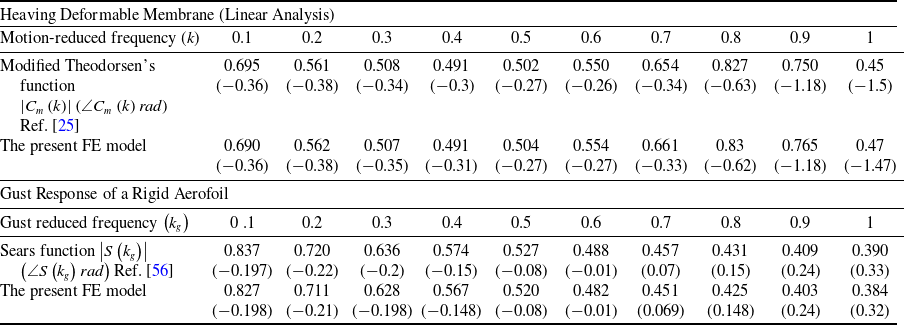
The verification of the present finite element model and the code implementation is done by considering two cases. The first case is a flexible membrane aerofoil with a tension coefficient of 2.5 experiencing a heaving harmonic motion. The ratio between the unsteady circulatory lift of the deformable membrane to the quasi-steady lift is defined by Tiomkin and Jaworski [Reference Tiomkin and Jaworski25] as the modified membrane Theodorsen’s function
 ${C}_{m}\left(k\right)$
which is compared with the present FE formulation using a linear structural model. The second case is the circulatory lift of a rigid flat plate under a sinusoidal gust loading, which is modeled by the well-known Sears function
 $S\left({k}_{g}\right)$
[Reference Bisplinghoff, Ashley and Halfman56]. The analysis is done by discretising the aerofoils into 50 elements. It can be seen from the results in Table 1 that the present model is in a good agreement with the published results.
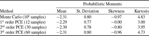
The uncertainty quantification code is verified by comparing the results of the PCE code with the standard Monte Carlo simulation for the standard short column test function given by the following equation [60]:
 \begin{align}f=1-\frac{4\mathbb{M}}{1125\mathbb{Y}}-\frac{{\mathbb{P}}^{2}}{5625{\mathbb{Y}}^{2}}\end{align}
Verification of the present FE model against published results of deformable membrane aerofoils and rigid flat aerofoil

The uncertain variables (
 $\mathbb{M},\mathbb{P}\,\text{and}\,\mathbb{Y}$
) are normal random variables with the following parameters:
 $\mathbb{M}\sim N\left(2000,400\right),\mathbb{P}\sim N\left(500,100\right)\,and\,\mathbb{Y}\sim N\left(5,0.5\right)$
. The probabilistic moments of the function are given in Table 2 that shows good agreement between the PCE with Latin hyper cube sampling and the Monte Carlo simulation with 106 samples.
Verification of the PCE code against the traditional Monte Carlo simulation for the short column test function

4.0 Results and Discussions
This section presents a parametric uncertainty aeroelastic analysis of a membrane aerofoil. When investigating the effect of one parameter, the rest of the parameters assume the following values; the considered membrane has a chord length of 1 m and is subjected to a free stream with a speed of
 ${V}_{\infty }=15\text{}\text{m}/\text{s}$
and an air density of
 ${\rho }_{\infty }=1.225\text{}\text{kg}/{\text{m}}^{3}$
. The membrane is supported by two springs at the leading edge and the trailing edge as shown in Fig. 1 with
 ${k}_{LE}=\Re *4000\text{}\text{N}/\text{m}$
and
 ${k}_{TE}=4000\text{}\text{N}/\text{m}$
, where
 $\Re $
is the spring ratio and has a value of 0.6. The membrane is made of material with an elastic modulus of
 $E=10\text{}\text{MPa}$
and has a thickness of
 $h=1\text{}\text{mm}$
. The initial tension force coefficient applied to the membrane of
 ${C}_{T}=2$
. The tension coefficient is defined as the ratio between the initial tension force and the free stream dynamic pressure (
 ${C}_{T}=T/c{q}_{\infty }$
). All of the considered uncertain variables follow Gaussian distributions with a coefficient of variation (CoV =
 $\sigma /\mu $
) of 0.1.
4.1 The static uncertain aeroelastic analysis
The effect of the input parameters’ uncertainty on the aerofoil’s static lift coefficient (
 ${C}_{L}$
) and moment coefficient (
 ${C}_{M}$
) about the quarter chord is studied in this section. Five random inputs are considered: the tension coefficient (which actually represents the uncertainty in the initial tension force and the free stream speed), the membrane elastic modulus, the stiffness coefficients of the two support springs and the angle-of-attack. Initially, the individual effect of each uncertain input is presented, followed by the combined effects of all uncertain inputs. Starting with the uncertain tension coefficient effect, Fig. 2(a) shows the variation of the uncertainty level (represented by the coefficient of variation) in the aerofoil lift coefficient and moment coefficient with respect to the mean tension force coefficient. It can be seen that the uncertainty in the aerodynamic coefficients strongly depends on the mean tension force coefficient with a peak at a moderate mean tension force coefficient value (around 2.25). This can be explained by Fig. 3 that shows the fact that at high mean tension coefficients, the membrane becomes very stiff resulting in small variations in the aerodynamic coefficients due to the tension coefficient uncertainty. On the other hand, for low mean tension coefficients, the 6-sigma range of the tension coefficient is small, which leads to small variations in the aerodynamic coefficients, and at the same time, the mean aerodynamic coefficients are high due to the increased membrane deformation which leads to low uncertainty levels (low CoV). The nonlinear stiffening effect represented by the elastic modulus also plays an important role for moderate tension coefficient values, but for low tension coefficient values (
 ${C}_{T} \lt 1$
) and high-tension coefficient values (
 ${C}_{T} \gt 4$
), this role becomes insignificant. The peak of the lift coefficient uncertainty quadruples as the membrane elastic modulus decreases 40 times from 40 MPa to 1 MPa, while the peak of the moment coefficient uncertainty only doubles. It can also be concluded that the uncertainty in the moment coefficient is more sensitive to the uncertainty in the tension coefficient compared to the uncertainty in the lift coefficient. For an elastic modulus of 1 MPa, the uncertainty level in the moment coefficient is triple the uncertainty level in the tension coefficient, while the uncertainty level in the lift coefficient is double the uncertainty level in the tension coefficient.
The variation of the lift and moment CoV with respect to the mean tension force coefficient (
 $\boldsymbol{\sigma}_{{C}_{T}}/\boldsymbol{\mu}_{{C}_{T}}=0.1$
) (a) for different deterministic elastic modulus values, (b) for different deterministic angles of attack and (c) for different deterministic spring ratios.

The variation of the lift and moment coefficients (deterministic analysis) with respect to the initial tension force different mean values of the tension force (a) lift coefficient (b) moment coefficient.

Similarly, the effects of the angle-of-attack and the springs’ stiffness ratio on the uncertainty in the aerodynamic coefficients due to the uncertain tension coefficient are shown in Fig. 2(b) and (c). Smaller angles of attack cause higher uncertainty levels in the aerodynamic coefficients, while the spring stiffness ratio has minimal effect except for the lift coefficient with a high mean tension coefficient (
 ${C}_{T} \gt 3$
). Figures 4 and 5 show the probability density functions (histograms) of the lift coefficient and moment coefficient due to uncertain tension coefficient for different membrane’s elastic modulus. For low elastic modulus, the PDFs of the aerodynamic coefficients are highly skewed similar to a Weibull distribution and then approach the Gaussian distribution as the modulus increases.
The histogram of the aerofoil lift coefficient due to the uncertain tension coefficient (
 $\boldsymbol{\mu}_{{C}_{T}}=2,\boldsymbol{\sigma}_{{C}_{T}}/{\mu }_{{C}_{T}}=0.1$
) for different elastic modulus values. (a)
 $E=1\,\text{MPa}$
, (b)
 $E=5\,\text{MPa}$
, (c)
 $E=10\,\text{MPa}$
and (d)
 $E=30\,\text{MPa}$
.

The histogram of the aerofoil moment coefficient due to the uncertain tension coefficient (
 $\boldsymbol{\mu}_{{C}_{T}}=2,\boldsymbol{\sigma}_{{C}_{T}}/{\mu }_{{C}_{T}}=0.1$
) for different elastic modulus values. (a)
 $E=1\,\text{MPa}$
, (b)
 $E=5\,\text{MPa}$
, (c)
 $E=10\,\text{MPa}$
and (d)
 $E=30\,\text{MPa}$
.

Moving to the effect of the uncertain elastic modulus, Fig. 6(a) shows the variation of the uncertainty levels in the aerodynamic coefficients with respect to the elastic modulus mean value for different deterministic tension coefficients. The uncertain modulus has a much lower effect on the aerodynamic coefficient compared to the effect of the uncertain tension coefficient. Approximately, for tension coefficients less than 2, the uncertainty levels in the aerodynamic coefficients decrease as the mean value of the elastic modulus increases, and vice versa for tension coefficients greater than 2. For certain cases, the mean elastic modulus seems to have no effect on the uncertainty of the lift coefficient or the moment coefficient. This discrepancy in the effect can be explained by examining how the nonlinear stiffening effect contributes to the deformation of the membrane and subsequently to the aerodynamic coefficients. For low tension coefficients (
 ${C}_{T} \lt 2$
), the membrane deformation tends to be large, and the nonlinear stiffening effect is significant, so for low mean Young’s modulus, the deformation is large and more sensitive to the Young’s modulus value, but as the mean Young’s modulus increases, the deformation decreases and becomes less sensitive to the Young’s modulus value. On the other hand, for large tension coefficient (
 ${C}_{T} \gt 2$
), the deformation tends to be small and the linear stiffness is more dominant when the Young’s modulus is low which justifies the negligible CoV, but as the mean Young’s modulus increases, the nonlinear stiffening effect increases even for small deformation which increases the deformation sensitivity with respect to the Young’s modulus.
The effect of the angle-of-attack on the aerodynamic coefficients due to uncertain elastic modulus is shown in Fig. 6(b). Unlike the case of the uncertain tension coefficient, the maximum uncertainty level in the aerodynamic coefficient is half the uncertainty level in the elastic modulus. The effect of the springs’ ratio is negligible as for the case of the uncertain tension coefficient, so it will not be repeated again. The membrane elastic modulus does not necessarily have a uniform value along the chord length, then the elastic modulus can be modeled as a random field instead of a random variable. Table 3 shows the effect of the random field correlation length (
 ${\unicode{x1D55D}}_{c}$
) on the aerodynamic coefficients’ uncertainty. As the correlation length decreases, the uncertainty also decreases in a cubic relation. For a correlation length of 0.1
 $C$
, the uncertainty drops to half compared to the case of random variable modeling.
The effect of the elastic modulus random field correlation length on the uncertainty in the aerodynamic coefficients. (
 ${C}_{T}=1,\alpha ={3}^{o}$
)

R.V. stands for random variable representation.
The variation of the lift and moment CoV with respect to the mean elastic modulus (
 $\boldsymbol{\sigma}_{E}/\boldsymbol{\mu}_{E}=0.1$
) (a) for different deterministic initial tension coefficients, and (a) for different deterministic angles of attack.

The third and fourth random inputs to the aeroelastic system are the spring stiffness coefficients of the trailing and leading edges, which represent the uncertainty in the underlying structure that supports the membrane aerofoil. These two coefficients can be probabilistically correlated with a correlation coefficient (
 $-1\le {\rho }_{c}\le 1$
). Figure 7(a) show the effects of the uncertain springs’ stiffness coefficients on the lift and moment coefficients for different spring ratios. It can be seen that the lift is the one affected by the spring stiffness uncertainty, while the moment has negligible uncertainty because the moment is mainly affected by the membrane camber caused by the deformation and not by the end points deflections. The highest uncertainty in the lift occurs with inversely perfectly correlated springs’ coefficients (
 ${\rho }_{c}=-1$
) and then decreases as the correlation increases. Additionally, increasing the spring ratio reduces the uncertainty in the lift coefficient. This is because increasing the spring ratio leads to the reduction of the angle-of-attack, and hence the lift becomes less sensitive to the spring stiffness uncertainty. Figure 7(b) and (c) show the effect of the tension coefficient and the angle-of-attack on the uncertainty of the aerodynamic due to the uncertain springs’ stiffness coefficients. The reason that perfectly correlated springs’ stiffness coefficients lead to a negligible uncertainty in the aerodynamic coefficients is the fact that changing the springs’ stiffness, in the case of perfect correlation, will mainly change the rigid body translation of the aerofoil upward or downward, which does not affect the aerodynamic coefficients. The effect of the elastic modulus value is negligible, so there is no need to present it here. Similar to the previous case of the uncertain elastic modulus, the uncertainty level in the aerodynamic coefficients is, at most, less than the half of the uncertainty level in the spring stiffness coefficients.
The effect of the correlation coefficient of the uncertain springs’ coefficients (
 $\boldsymbol{\sigma}_{k}/\boldsymbol{\mu}_{k}=0.1$
) on the aerodynamic coefficients CoV (a) for different spring ratios, (b) for different deterministic initial tension coefficients and (c) for different deterministic angles of attack.

The last and fifth uncertain random variable to be considered in this section is the uncertain free stream angle-of-attack. Figure 8 shows the variation of the uncertainty in the aerodynamic coefficients with respect to the mean angle-of-attack. Opposite to the case of the uncertain elastic modulus, for tension coefficients less than 2, the uncertainty in the aerodynamic coefficients increases as the mean angle-of-attack increases, and vice versa for tension coefficients greater than 2. It can be seen from Fig. 8(a) that the uncertainty level in the aerodynamic coefficients can reach the same uncertainty level in the angle-of-attack for low-mean angles of attack and high-tension coefficients. The deterministic value of the elastic modulus has an effect on the uncertainty level in the aerodynamic coefficients as the mean angle-of-attack changes only when the elastic modulus is very low about 1 MPa as can be seen from Fig. 8(b).
The variation of the lift and moment CoV with respect to the mean angle-of-attack (
 $\boldsymbol{\sigma}_{\alpha }/\boldsymbol{\mu }_{\alpha}=0.1$
) (a) for different deterministic initial tension coefficients and (b) for different deterministic elastic moduli.

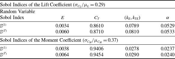
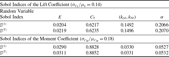
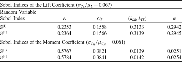
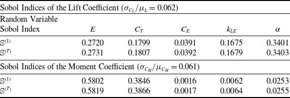
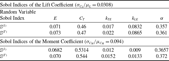
Now the combined effects of all five random input variables can be analysed through the sensitivity analysis given in Tables 4, 5, 6 and 7. The results in Tables 4, 5 and 6 are for the perfectly inversely correlated spring stiffness coefficients to maximise their contribution, while no correlation is assumed in Table 7. It can be seen that the contribution of each random variable depends mainly on the mean tension coefficient value and the elastic modulus as shown in the three cases in Tables 4, 5 and 6. Also, it seems that the interaction terms in the PCE have negligible effect as the first-order Sobol indices are almost equal to the total Sobol indices. Each uncertain input can have more effect on one aerodynamic coefficient than the other. For example, in case 3 in Table 6, the elastic modulus contributes with a round 24% in the uncertainty of the lift coefficient and 58% in the uncertainty of the moment coefficient, while the angle-of-attack and the springs’ stiffness contribute with around 30% in the uncertainty of the lift and have a negligible effect on the moment coefficient. Comparing the results in Tables 6 and 7, the contribution of the spring stiffness coefficients in the lift uncertainty drops by 30% when no correlation is assumed, and the leading-edge stiffness coefficient has the dominant effect (four times the contribution of the trailing edge stiffness coefficient).
The sensitivity analysis of the uncertain static aeroelastic system due to all five random inputs with perfectly inversely correlated springs’ coefficients; case 1 (
 $\text{}{\mu }_{{C}_{T}}=2,{}\text{}{\mu }_{E}=1\,{\text{MPa}}_{\text{}},{\mu }_{\alpha }={2}^{o},\text{}{\mu }_{{k}_{LE}}{}_{\text{}}={\mu }_{{k}_{TE}}=4000\,\text{N}/\text{m},\text{}\Re =0.6$
,
 ${\rho }_{c}=-1$
)

The sensitivity analysis of the uncertain static aeroelastic system due to all five random inputs with perfectly inversely correlated springs’ coefficients; case 2 (
 $\text{}{\mu }_{{C}_{T}}=2,{}\text{}{\mu }_{E}=10\,{\text{MPa}}_{\text{}},\text{}{\mu }_{\alpha }={2}^{},\text{}{\mu }_{{k}_{LE}}{}_{\text{}}={\mu }_{{k}_{TE}}=4000\,\text{N}/\text{m},\text{}\Re =0.6$
,
 ${\rho }_{c}=-1$
)

The sensitivity analysis of the uncertain static aeroelastic system due to all five random inputs with perfectly inversely correlated springs’ coefficients; case 3 (
 $\text{}{\mu }_{{C}_{T}}=1,{}\text{}{\mu }_{E}=20\,{\text{MPa}}_{\text{}},{\mu }_{\alpha }={2}^{o},\text{}{\mu }_{{k}_{LE}}{}_{\text{}}={\mu }_{{k}_{TE}}=4000\,\text{N}/\text{m},\text{}\Re =0.6$
,
 ${\rho }_{c}=-1$
)

The sensitivity analysis of the uncertain static aeroelastic system due to all five random inputs with uncorrelated springs’ coefficients (
 $\text{}{\mu }_{{C}_{T}}=1,\text{}{\mu }_{E}=20\,{\text{MPa}}_{\text{}},{}{\mu }_{\alpha }={2}^{o},\text{}{\mu }_{{k}_{LE}}{}_{\text{}}={\mu }_{{k}_{TE}}=4000\text{}\text{N}/\text{m},\text{}\Re =0.6$
,
 ${\rho }_{c}=0$
)

4.2 The dynamic uncertain aeroelastic analysis
This section deals with the uncertain dynamic response of the membrane aerofoil under sinusoidal gust loadings. The gust is assumed to have a vertical speed amplitude of 0.5 m/s and a frequency of 1 Hz. The fourth-order Runge Kutta method is used for the time simulation of the aeroelastic system with a time step of 0.002 s. Figure 9 shows the variation of the uncertainty level in the lift coefficient amplitude (
 ${\overline{C}}_{L}$
) and the moment coefficient amplitude (
 ${\overline{C}}_{M}$
) due to the uncertain tension coefficient. Similar to the static case, the moment coefficient is more sensitive to the uncertainty in the tension coefficient, but the maximum level of uncertainty is far less than the static case for the same uncertainty level in the tension coefficient. Opposite to the static case, there is a dip in the uncertainty level of the aerodynamic coefficients for mean tension coefficients between 2 and 2.5. This dip can be justified by investigating the variations of the aerodynamic coefficients’ amplitudes with respect to the tension coefficient as shown in Fig. 10, which shows that the maximum amplitude occurs for a tension coefficient around 2.25. Therefore, it is logical for the uncertainty to reduce as the mean tension coefficient approaches this value. It was found that this behaviour is unchanged for several angles of attack, but the peak amplitude increases slightly for lower angles of attack. Also, the behaviour (not the values) is unaffected by the gust amplitude and for gust frequencies range 0 Hz- 2.8 Hz, which corresponds to a gust reduced frequency range 0–0.3. The probability density functions (histograms) of the lift coefficient amplitude for different mean tension coefficient values are shown in Fig. 11. These histograms are obtained using up to a 6th-order PCE and the LHS method. It can be seen that the probability nature strongly depends on the mean tension coefficient, and it varies from a Gaussian distribution for very low or very high mean tension coefficients to an exponential-like distribution for a mean tension coefficient near 2.
The variation of the lift and moment amplitudes CoV with respect to the mean tension force coefficient (
 $\boldsymbol{\sigma }_{{C}_{T}}/\boldsymbol{\mu }_{{C}_{T}}=0.1$
) under a sinusoidal gust loading for different deterministic elastic modulus values (a) lift amplitude CoV, (b) moment amplitude CoV.

(deterministic analysis) The variation of the lift and moment coefficients’ amplitudes with respect to the tension coefficient under a sinusoidal gust loading (
 ${W}_{g}=0.5\text{}\text{m}/\text{s},\alpha ={2}^{o}$
) for different elastic modulus values (a) lift coefficient amplitude (b) moment coefficient amplitude.

The histograms of the membrane aerofoil lift coefficient amplitude due to uncertain tension coefficient (
 $\boldsymbol{\sigma}_{{C}_{T}}/\boldsymbol{\mu}_{{C}_{T}}=0.1,E=1\,\textrm{MPa}$
) under a sinusoidal gust loading (a)
 ${\mu }_{{C}_{T}}=1$
, (b)
 ${\mu }_{{C}_{T}}=1.6$
, (c)
 ${\mu }_{{C}_{T}}=2$
, (d)
 ${\mu }_{{C}_{T}}=2.5$
, (e)
 ${\mu }_{{C}_{T}}=3$
(f)
 ${\mu }_{{C}_{T}}=5$
.

Figure 12 shows the uncertainty in the amplitudes of the aerodynamic coefficient due to the uncertain elastic modulus. The uncertainty in the lift coefficient is considered negligible, and the uncertainty in the moment coefficient amplitude is small with a maximum value of 25% of the uncertainty in the elastic modulus. It can be observed that the uncertainty reaches the maximum value when the tension coefficient is near 2, which is opposite to the previous case of the uncertain tension coefficient, and it is almost invariant with respect to the mean elastic modulus value. Moving on to the effects of uncertain spring coefficients, Fig. 13 shows the variation of the uncertainty in the lift amplitude and the moment amplitude with the springs’ correlation coefficient. The effect is exactly the same as in the case of the uncertain elastic modulus. But unlike the static case, the springs’ uncertainty has an effect on the moment amplitude. This may be due to the effect of the added mass in the unsteady pressure distribution. The effect of the mean spring coefficient is shown in Fig. 14, which indicates inverse linear relationships between the mean spring coefficient value and the uncertainty in the aerodynamic coefficients’ amplitudes. Interestingly, as the tension coefficient increases, the uncertainty in the lift amplitude due to the uncertain springs’ coefficients increases, while the moment amplitude uncertainty drops when the tension coefficient is near 2 and then increases as the tension increases. Finally, the effect of the uncertain angle-of-attack is shown in Fig. 15. The uncertainty in the aerodynamic coefficients’ amplitudes increases as the mean angle-of-attack increases. Similar to the case of uncertain elastic modulus, the maximum uncertainty occurs when the tension coefficient is near 2.
The variation of the lift and moment amplitudes CoV with respect to the mean elastic modulus (
 ${\sigma }_{E}/{\mu }_{E}=0.1$
) under a sinusoidal gust loading for different deterministic initial tension coefficients (a) lift amplitude CoV (b) moment amplitude CoV.

The variation of the lift and moment amplitudes CoV with respect to the correlation coefficient of the uncertain springs’ coefficients (
 ${\sigma }_{k}/{\mu }_{k}=0.1$
) under a sinusoidal gust loading for different spring ratios (a) lift amplitude CoV (b) moment amplitude CoV.

The variation of the lift and moment amplitudes CoV with respect to the mean spring stiffness coefficient (
 ${\sigma }_{k}/{\mu }_{k}=0.1,\text{}{\rho }_{c}=-1$
,
 ${k}_{LE}=\Re *k$
and
 ${k}_{TE}=k$
,
 $\Re =0.6$
) under a sinusoidal gust loading for different initial tension coefficients (a) lift amplitude CoV (b) moment amplitude CoV.

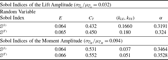
The last point to be addressed in this paper is the uncertainty sensitivity analysis of the membrane aerofoil under sinusoidal gust loading. The mean tension coefficient is chosen to be 2 to increase the contribution of the other parameters. Tables 8 and 9 show the sensitivity analysis results for the case of correlated and uncorrelated spring coefficients, respectively. The contribution of each uncertain input is similar to the static case with an increased effect of the angle-of-attack.
The sensitivity analysis of the uncertain dynamic aeroelastic system due to all five random inputs with perfectly inversely correlated springs’ coefficients (
 $\text{}{\mu }_{{C}_{T}}=2,\text{}{\mu }_{E}=10\,{\text{MPa}}_{\text{}},{\mu }_{\alpha }={2}^{o},\text{}{\mu }_{{k}_{LE}}{}_{\text{}}={\mu }_{{k}_{TE}}=4000\text{}\text{N}/\text{m},\text{}\Re =0.6$
,
 ${\rho }_{c}=-1$
)

The sensitivity analysis of the uncertain dynamic aeroelastic system due to all five random inputs with uncorrelated springs’ coefficients (
 $\text{}{\mu }_{{C}_{T}}=1,{}{\mu }_{E}=20\,{\text{MPa}}_{\text{}},{\mu }_{\alpha }={2}^{o},\text{}{\mu }_{{k}_{LE}}{}_{\text{}}={\mu }_{{k}_{TE}}=4000\text{}\text{N}/\text{m},\text{}\Re =0.6$
,
 ${\rho }_{c}=0$
)

The variation of the lift and moment amplitudes CoV with respect to the mean angle-of-attack (
 ${\sigma }_{}/{\mu }_{\alpha }=0.1$
) under a sinusoidal gust loading for different initial tension coefficients (a) lift amplitude CoV, (b) moment amplitude CoV.

5.0 Conclusions
The uncertain static and dynamic nonlinear aeroelasticity of membrane aerofoils is studied in this paper. The uncertain input variables are the initial tension coefficient, the membrane elastic modulus, the stiffness of the supporting springs at the trailing edge and the leading edge and the free stream angle-of-attack. The aerofoil moment coefficient is more sensitive to uncertainties in the inputs compared to the lift coefficient (experiencing higher uncertainty levels). Additionally, the uncertainty levels in the aerodynamic coefficients for the static case are higher than the dynamic case.
The tension coefficient plays the master role in the uncertainties of the aerodynamic coefficients and in the contribution of the other uncertain inputs. There is a linear relationship between the uncertainty levels of the aerodynamic coefficients and the uncertainty levels of the random inputs. The probability distribution functions of the aerodynamic coefficients strongly depend on the case study (static or dynamic) and the mean values of the input parameters.
For the static case, the probability distribution functions can vary from a Gaussian distribution to a highly skewed Weibull distribution, while for the dynamic case, the probability distribution functions can have any general distribution depending mainly on the mean tension coefficient value. The maximum uncertainty levels in the aerodynamic coefficients due to each random input separately can reach multiples of the uncertainty levels of the tension coefficient, similar to the uncertainty level of the angle-of-attack, and half the uncertainty levels of the supporting springs and the elastic modulus.
The mean tension coefficient range between 2 and 3 is the most critical range, which causes maximum uncertainty levels in the aerodynamic coefficients for the static case, but minimum uncertainty levels for the dynamic case. The correlation between the leading-edge spring and the trailing edge spring has a significant effect with maximum uncertainty is reached when they are inversely perfectly correlated. The uncertainty of the leading-edge supporting spring has four times the effect of the uncertainty of the trailing-edge supporting spring.
Conflict of interests
The author states that there is no conflict of interest of any kind regarding the work presented in this paper.
Appendix
A.1 Aerodynamic matrices
By defining a coordinate transformation as
 ${x}^{*}=-cos\theta $
, then the finite element formulation of the quasi-steady aerodynamic loading can be written as follows [Reference Hussein26, Reference Hussein27]:
 \begin{align}{[{A}_{\mathcal{Q}\mathcal{S}}^{1}]}^{}{}_{2\times \left({n}_{s}+1\right)}=4{l}_{e}\int_{0}^{1}\lfloor{N}_{s}\rfloor{}^{T}\text{}\begin{array}{ccc}\Big\lfloor\frac{1+\mathrm{cos}\left(\theta \right)}{\mathrm{sin}\left(\theta \right)} {} \mathrm{sin}\left(\theta \right) {} \begin{array}{cc}\begin{array}{cc}\quad {}\quad {} \dots\,\,\, \end{array} {} \mathrm{sin}\left({n}_{a}\theta \right)\end{array}\Big\rfloor\end{array}[{\mathbb{P}}_{s}]ds\end{align}
 \begin{align}{[{A}_{\mathcal{Q}\mathcal{S}}^{2}]}^{e}{}_{2\times \left({n}_{s}+1\right)}=4{l}_{e}\int_{0}^{1}\lfloor{N}_{s}\rfloor{}^{T}\text{}\begin{array}{ccc}\Big\lfloor\frac{1+\mathrm{cos}\left(\theta \right)}{\mathrm{sin}\left(\theta \right)} {} \mathrm{sin}\left(\theta \right) {} \begin{array}{cc}\begin{array}{cc}\quad\quad\!\! \dots\,\, \end{array} {} \mathrm{sin}\left({n}_{a}\theta \right)\end{array}\Big\rfloor\end{array}[{\mathbb{P}}_{d}]ds\end{align}
 \begin{align}{\left\{{f}_{\mathcal{Q}\mathcal{S}}\right\}}^{e}{}_{2\times 1}=\text{}4{l}_{e}\int_{0}^{1}\alpha \lfloor{N}_{s}\rfloor{}^{T}\text{}\frac{1+\mathrm{cos}\left(\theta \right)}{\mathrm{sin}\left(\theta \right)}ds\end{align}
 \begin{align}{[{\mathbb{P}}_{s}]}_{{n}_{a}\times \text{}({n}_{s}+1)}=\frac{{\mathcal{C}}^{\left(m\right)}}{\pi }\frac{1}{{l}_{e}}\int_{{\theta }_{j1}}^{\theta {j}_{2}}\lfloor{N}_{s,s}\rfloor\mathrm{cos}\left(m\theta \right)d\theta ,m=1\to {n}_{a}\,and\,j=1\to {n}_{s}\end{align}
 \begin{align}{[{\mathbb{P}}_{d}]}_{{n}_{a}\times \text{}({n}_{s}+1)}=\frac{{\mathcal{C}}^{\left(m\right)}}{\pi }\int_{{\theta }_{j1}}^{\theta {j}_{2}}\lfloor{N}_{s}\rfloor\mathrm{cos}\left(m\theta \right)d\theta\end{align}
 \begin{align}{\mathcal{C}}^{\left(m\right)}=\bigg\{\begin{array}{c}\begin{array}{cc}-1 {} m=0\end{array}\\ \begin{array}{cc}\text{}2 {} m\ne 0\end{array}\end{array}\\[-3pt]\nonumber\end{align}
The added mass and the wake-effect aerodynamic loading finite element matrices, which represents the interaction between any two elements along the chord, can be written as follows:
 \begin{align}{[{A}_\mathcal{M}^{1}]}^{e}{}_{2\times 2}=\frac{4{l}_{e}^{2}}{\pi {b}^{2}}\underset{0}{\overset{1}\int}\underset{0}{\overset{1}\int}\bigg\lceil\begin{array}{c}1-s\\ s\end{array}\bigg\rceil\Lambda\left({x}^{*},{\xi }^{*}\right)\text{}\lfloor\begin{array}{cc}1-\eta\quad {} \eta \end{array}\rfloor\ ds\ d\eta ,\end{align}
 \begin{align}{[{A}_\mathcal{M}^{2}]}^{e}{}_{2\times 2}=-\frac{4{l}_{e}}{\pi b}\underset{0}{\overset{1}\int}\underset{0}{\overset{1}\int}\bigg\lceil\begin{array}{c}1-s\\ s\end{array}\bigg\rceil\Lambda\left({x}^{*},{\xi }^{*}\right)\ [\begin{array}{cc}-1\quad 1\end{array}]\ ds\ d\eta\end{align}
 \begin{align}{\left\{{f}_\mathcal{M}\right\}}^{e}{}_{2\times 1}=\frac{4{l}_{e}^{2}}{\pi b}\underset{0}{\overset{1}\int}\underset{0}{\overset{1}\int}\dot{\alpha }\bigg\lceil\begin{array}{c}1-s\\ s\end{array}\bigg\rceil\Lambda\left({x}^{*},{\xi }^{*}\right)ds\ d\eta\end{align}
 \begin{align}{[{A}_{\mathcal{W}}^{1}]}^{e}{}_{2\times 2}=\frac{4{l}_{e}^{2}}{\pi {b}^{2}}\underset{0}{\overset{1}\int}\underset{0}{\overset{1}\int}\bigg\lceil\begin{array}{c}1-s\\ s\end{array}\bigg\rceil\sqrt{\frac{1-{x}^{*}}{1+{x}^{*}}}\sqrt{\frac{1+{\xi }^{*}}{1-{\xi }^{*}}}\,\,\,\,\lfloor\begin{array}{cc}1-\eta\quad\eta \end{array}\rfloor\ ds\ d\eta\end{align}
 \begin{align}{[{A}_{\mathcal{W}}^{2}]}^{e}{}_{2\times 2}=\frac{4{l}_{e}}{\pi b}\underset{0}{\overset{1}\int}\underset{0}{\overset{1}\int}\bigg\lceil\begin{array}{c}1-s\\ s\end{array}\bigg\rceil\sqrt{\frac{1-{x}^{*}}{1+{x}^{*}}}\sqrt{\frac{1+{\xi }^{*}}{1-{\xi }^{*}}}\,\,\,[\begin{array}{cc}-1\quad1\end{array}]\ ds\ d\eta\end{align}
 \begin{align}{\left\{{f}_{\mathcal{W}}\right\}}^{e}{}_{2\times 1}=\frac{-4{l}_{e}^{2}}{\pi b}\underset{0}{\overset{1}\int}\underset{0}{\overset{1}\int}\alpha \bigg\lceil\begin{array}{c}1-s\\ s\end{array}\bigg\rceil\sqrt{\frac{1-{x}^{*}}{1+{x}^{*}}}\sqrt{\frac{1+{\xi }^{*}}{1-{\xi }^{*}}}\ ds\ d\eta,\end{align}
A.2. PCE orthogonal functions for Gaussian distribution (Hermite polynomials)
 \begin{align}\nonumber{\mathbb H}_{n}\left(Z\right)&=Z{\mathbb H}_{n-1}\left(\right)-\text{}\left(-1\right){\mathbb H}_{n-2}\left(Z\right),\nonumber\\{\mathbb H}_{o}\left(Z\right)&=1,\nonumber\\ {\mathbb H}_{1}\left(Z\right)&=Z,\nonumber\\ {\mathbb H}_{2}\left(Z\right)&={Z}^{2}-1,\nonumber\\{\mathbb H}_{3}\left(Z\right)&={Z}^{3}-3,\nonumber\\ {\mathbb H}_{4}\left(Z\right)&={Z}^{4}-6{Z}^{2}+3,\nonumber\\ {\mathbb H}_{5}\left(Z\right)&={Z}^{5}-10{Z}^{3}+15Z,\nonumber\\ {\mathbb H}_{6}\left(Z\right)&={Z}^{6}-15{Z}^{4}+45{Z}^{2}-15\end{align}
A.3. KLE basis functions for exponential covariance
 \begin{align}\psi \left({x}^{*}\right)=\left\{\begin{array}{c}\begin{array}{cc}\frac{cos({\Omega}_{i}{x}^{*})}{\sqrt{1+\frac{sin\left(2{\Omega}_{i}\right)}{2{\Omega}_{i}}}} {} i=1,3,5,\dots \end{array}\\ \begin{array}{cc}\frac{sin({\Omega}_{i}{x}^{*})}{\sqrt{1-\frac{sin\left(2{\Omega}_{i}\right)}{2{\Omega}_{i}}}} {} i=2,4,6,\dots \end{array}\end{array}\right.\end{align}
 \begin{align}{\lambda }_{i}=\frac{2{\unicode{x1D55D}}_{c}^{*}}{1+{\unicode{x1D55D}}_{c}^{*}{}^{2}{\Omega}_{i}^{2}},\text{}{\unicode{x1D55D}}_{c}^{*}=\frac{{\unicode{x1D55D}}_{c}}{C}\end{align}
Where
 ${\omega}_\textrm{i}$
is obtained by solving the following equation:
 \begin{align}\left(\Omega+\frac{1}{{\unicode{x1D55D}}_{c}^{*}}tan\left(\Omega\right)\right)\left(\frac{1}{{\unicode{x1D55D}}_{c}^{*}}-\Omega tan\left(\Omega\right)\right)=0.\end{align}