2 Spectral vector determines D

Let q be a prime power and $f \in {\mathbb {F}}_q[x]$ a monic polynomial. As we explain in [Reference Mináč, Nguyen and Tân14, Section 6], there is a direct analogy between the character theory of ${\mathbb {Z}}/n$ and that of ${\mathbb {F}}_q[x]/f$ . More specifically, while the character theory of ${\mathbb {Z}}/n$ can be fully described once we fix a primitive nth root of unity, the character theory of ${\mathbb {F}}_q[x]/f$ is similarly determined by a fixed nondegenerate functional on ${\mathbb {F}}_q[x]/f$ . As a result, the spectra of gcd-graphs in both cases have explicit descriptions via Ramanujan sums. For the case of gcd-graphs over ${\mathbb {Z}}$ , we refer readers to [Reference Klotz and Sander10, Section 4]. For ${\mathbb {F}}_q[x]$ , we now recall the definition of the Ramanujan sums that describe the spectra of gcd-graphs.

Definition 2.1 (See [Reference Mináč, Nguyen and Tân14, Section 6.2]).

Let $f \in {\mathbb {F}}_q[x]$ be a monic polynomial. For each $g \in {\mathbb {F}}_q[x]$ , the Ramanujan sum $c(g,f)$ is defined as

$$ \begin{align*} c(g,f) = c_{\psi}(g,f) = \sum_{a \in ({\mathbb{F}}_q[x]/f)^{\times}} \zeta_p^{{\text{Tr}}(\psi(ga))}. \end{align*} $$

Here, $\psi : {\mathbb {F}}_q[x]/f \to {\mathbb {F}}_q$ is a nondegenerate functional on ${\mathbb {F}}_q[x]/f$ and ${\text {Tr}}: {\mathbb {F}}_q \to {\mathbb {F}}_p$ is the trace map.

While the above definition looks rather complicated, we can show that $c(g,f)$ has a simple expression almost analogous to the case of Ramanujan sums over ${\mathbb {Z}}$ . In particular, $c(g,f)$ does not depend on the choice of $\psi $ as long as we make sure that it is nondegenerate. More precisely, by [Reference Mináč, Nguyen and Tân14, Section 6.2], we have

(2-1) $$ \begin{align} c(g,f) = \mu(t) \dfrac{\varphi(f)}{\varphi(t)} \quad \text{where} \ t = \dfrac{f}{\gcd(f,g)}. \end{align} $$

Here, $\varphi (f)=|({\mathbb {F}}_q[x]/f)^{\times }|$ is the analog of the classical Euler function and $\mu (t)$ is the analog of the classical Mobius function (see [Reference Rosen16] for some further discussions about these functions).

The following definition is inspired by the work [Reference Sander and Sander18] of Sander and Sander on gcd-graphs over ${\mathbb {Z}}.$

Definition 2.2. Let ${\mathrm{Div}}(f)$ be the set of monic divisors of f. Let $D \subset {\mathrm{Div}}(f)$ such that $f \not \in D$ . The spectral vector of the gcd-graph $G_{f}(D)$ is defined to be the following vector:

$$ \begin{align*} \vec{\lambda}(f,D) = (\lambda_{g}(f,D) )_{g \in {\mathbb{F}}_q[x]/f}, \end{align*} $$

where

(2-2) $$ \begin{align} \lambda_{g} (f,D) = \sum_{d \in D} c\bigg(g, \frac{f}{d} \bigg). \end{align} $$

By the main result in [Reference Mináč, Nguyen and Tân14, Section 6], the components of this spectral vector are precisely the eigenvalues of $G_{f}(D)$ counted with multiplicity. The following theorem is a direct analog of [Reference Sander and Sander18, Theorem 1.2].

To prove Theorem 2.3, we adapt the strategy employed in [Reference Schlage-Puchta19], which deals with gcd-graphs over ${\mathbb {Z}}$ . More precisely, we introduce and study a matrix similar to that defined in [Reference Schlage-Puchta19]. Let $g,h \in {\mathbb {F}}_q[x]$ and $c(g,h)$ be the Ramanujan sum. Let $C_f = (c(g,h))_{g,h \in {\mathrm{Div}}(f)}.$ In [Reference Schlage-Puchta19, Theorem 1], the author solves the weak conjecture of Sander and Sander by showing that the determinant of $C_n$ is not zero. In the case of ${\mathbb {F}}_q[x]$ , we have a similar statement.

Proposition 2.4. Let $|f|$ be the norm of f; that is, $|f|$ is the order of the finite ring ${\mathbb {F}}_q[x]/f.$ Then,

$$ \begin{align*} \det(C_f)= \pm |f|^{({\tau(f)}/{2})} .\end{align*} $$

Here, $\tau (f)$ is the number of monic divisors of $f.$ In particular, $\det (C_f) \neq 0.$

We remark that the sign of $\det (C_f)$ depends on the ordering of ${\mathrm{Div}}(f).$ For our application, this sign is not important.

Proof. We proceed by induction on the number of monic irreducible factors of f. If $\deg f=0$ , then $f=1$ and $\det (C_1)=1$ . Now, let $\deg f>0$ and P be a monic irreducible polynomial coprime to f. Let n be a positive integer. Let $f_1,f_2,\ldots , f_r$ be the monic divisors of f; here, $r=\tau (f)$ . We list the monic divisors of $P^nf$ as

$$ \begin{align*} f_1,f_2,\ldots,f_r,Pf_1,Pf_2,\ldots,Pf_r, \ldots,P^2f_1,P^2f_2,\ldots,P^2f_r,\ldots, P^nf_1,P^nf_2,\ldots,P^nf_r. \end{align*} $$

Then, $C_{P^nf}$ is an $(n+1)\times (n+1)$ -block matrix

$$ \begin{align*} \begin{bmatrix} C_{00}&C_{01}&\cdots&C_{0n}\\ C_{10}&C_{11}&\cdots&C_{1n}\\ \vdots&\vdots&\cdots&\vdots\\ C_{n0}&C_{n1}&\cdots&C_{nn} \end{bmatrix}, \end{align*} $$

where $C_{ij}$ is an $r\times r$ -matrix whose $(k,l)$ -entry is

$$ \begin{align*} (C_{ij})_{kl}=c(P^id_k,P^jd_l). \end{align*} $$

Clearly, $C_{00}=C_f$ . If $j\geq i+2$ , then

$$ \begin{align*} c(P^id_k,P^jd_l)=\dfrac{\varphi(P^jd_l)}{\varphi\Big(\frac{P^jd_l}{\gcd(P^id_k,P^jd_l)}\Big)}\mu\bigg(\dfrac{P^jd_l}{\gcd(P^id_k,P^jd_l)}\bigg)=0. \end{align*} $$

This is because ${P^jd_l}/({\gcd (P^id_k,P^jd_l)})$ is divisible by $P^2$ .

If $j=i+1$ , then

$$ \begin{align*} \begin{aligned} c(P^id_k,P^jd_l)&=\dfrac{\varphi(P^jd_l)}{\varphi\Big(\frac{P^jd_l}{\gcd(P^id_k,P^jd_l)}\Big)}\mu\bigg(\dfrac{P^jd_l}{\gcd(P^id_k,P^jd_l)}\bigg)\\&=\dfrac{\varphi(P^{i+1})}{\varphi(P)} \dfrac{\varphi(d_l)}{\varphi\Big(\frac{d_l}{\gcd(d_k,d_l)}\Big)}\mu(P)\mu\bigg(\dfrac{d_l}{\gcd(d_k,d_l)}\bigg)\\&=-|P|^i \dfrac{\varphi(d_l)}{\varphi\Big(\frac{d_l}{\gcd(d_k,d_l)}\Big)}\mu\bigg(\dfrac{d_l}{\gcd(d_k,d_l)}\bigg)=-|P|^ic(d_k,d_l), \end{aligned} \end{align*} $$

and, hence, $C_{i,i+1}=-|P|^iC_f.$

If $j\leq i$ , then

$$ \begin{align*} \begin{aligned} c(P^id_k,P^jd_l)&=\dfrac{\varphi(P^jd_l)}{\varphi\Big(\frac{P^jd_l}{\gcd(P^id_k,P^jd_l)}\Big)}\mu\bigg(\dfrac{P^jd_l}{\gcd(P^id_k,P^jd_l)}\bigg)\\&=\dfrac{\varphi(P^j)\varphi(d_l)}{\varphi\Big(\frac{d_l}{\gcd(d_k,d_l)}\Big)} \mu\bigg(\dfrac{d_l}{\gcd(d_k,d_l)}\bigg) =\varphi(P^j)c(d_k,d_l), \end{aligned} \end{align*} $$

and, hence, $C_{ij}=\varphi (P^j)C_f$ . Thus,

$$ \begin{align*} C_{P^nf}= \begin{bmatrix} C_f&-C_f&0&0&\cdots&0\\C_f&\varphi(P)C_f&-|P|C_f&0&\cdots&0\\C_f&\varphi(P)C_f&\varphi(P^2)C_f&-|P|^2C_f&\cdots&0\\\vdots&\vdots&\vdots&\vdots\\C_f&\varphi(P)C_f&\varphi(P^2)C_f&\varphi(P^3)C_f&\cdots&-|P|^{n-1}C_f\\C_f&\varphi(P)C_f&\varphi(P^2)C_f&\varphi(P^3)C_f&\cdots&\varphi(P^n)C_f \end{bmatrix}. \end{align*} $$

Subtracting the nth row from the $(n+1)$ th row and noting that $\varphi (P^n)+|P|^{n-1}=|P^n|$ ,

$$ \begin{align*} \begin{aligned} \det (C_{P^nf})&=\pm \det\begin{bmatrix} C_f&-C_f&0&0&\cdots&0\\ C_f&\varphi(P)C_f&-|P|C_f&0&\cdots&0\\ C_f&\varphi(P)C_f&\varphi(P^2)C_f&-|P|^2C_f&\cdots&0\\ \vdots&\vdots&\vdots&\vdots\\ C_f&\varphi(P)C_f&\varphi(P^2)C_f&\varphi(P^3)C_f&\cdots&-|P|^{n-1}C_f\\ 0&0&0&0&\cdots&|P|^nC_f& \end{bmatrix}. \end{aligned}\end{align*} $$

Expanding along the last block row gives

$$ \begin{align*} \begin{aligned} \det (C_{P^nf})&=\pm |P|^{rn}\det(C_f)\det\begin{bmatrix} C_f&-C_f&0&0&\cdots&0\\ C_f&\varphi(P)C_f&-|P|C_f&0&\cdots&0\\ C_f&\varphi(P)C_f&\varphi(P^2)C_f&-|P|^2C_f&\cdots&0\\ \vdots&\vdots&\vdots&\vdots\\ C_f&\varphi(P)C_f&\varphi(P^2)C_f&\varphi(P^3)C_f&\cdots&\varphi(P^{n-1})C_f \end{bmatrix}. \end{aligned} \end{align*} $$

Repeating this argument, we obtain

$$ \begin{align*} \begin{aligned} \det (C_{P^nf}) &=\pm |P|^{rn}\det(C_f) |P|^{r(n-1)}\det(C_f)\cdots|P^r|\det(C_f)\\ &=\pm |P|^{({n(n+1)}/{2})\tau(f)}(\det C_f)^{n+1}. \end{aligned} \end{align*} $$

By the induction hypothesis,

$$ \begin{align*} \det (C_{P^nf})=\pm |P|^{({n(n+1)}/{2})\tau(f)}(|f|^{({\tau(f)}/{2})})^{n+1}=\pm(|P|^n|f|)^{({(n+1)\tau(f)}/{2})}=\pm|P^nf|^{({\tau(P^nf)}/{2})} \end{align*} $$

and we are done.

We can now give a proof of Theorem 2.3.

Proof. Assume that $G_{f}(D_1)$ and $G_{f}(D_2)$ have the same spectral vector $\vec {\lambda }(f,D_1) = \vec {\lambda }(f, D_2)$ . Then, the subvectors $(\lambda _{g} (f,D_1))_{g \mid f}$ and $(\lambda _{g} (f,D_2))_{g \mid f}$ indexed by divisors of f are also equal. For each $i \in \{1, 2\}$ , we define the following indicator vector of size $|\tau (f)| \times 1$ :

$$ \begin{align*} (v_i)_{h} = \begin{cases} 1 & \text{if } f/h \in D_i, \\ 0 & \text{if } f/h \not \in D_i. \\ \end{cases}\end{align*} $$

We then see that the vectors $(\lambda _{g} (f,D_1))_{g \mid f}$ (respectively $(\lambda _{g} (f,D_2))_{g \mid f}$ ) are precisely $C_f v_1$ (respectively $C_f v_2$ ). Since $C_f$ is invertible, we conclude that $v_1 = v_2$ and, therefore, $D_1 = D_2.$

3 Gcd-graphs associated with prime powers I: graph-theoretic properties of $G_{P^k}(D)$

In this section, we study the gcd-graphs $G_{f}(D)$ in the case where f is a prime power; that is, $f=P^k$ , where $P \in {\mathbb {F}}_q[x]$ is an irreducible polynomial and $k \geq 1.$ In this case, a subset D of ${\mathrm{Div}}(P^k)$ can be written uniquely in the form ${D = \{P^{k_1}, P^{k_2}, \ldots , P^{k_s}\}}$ , where

$$ \begin{align*} 0 \leq k_1 <k_2 < \cdots < k_s <k. \end{align*} $$

We fix this notation throughout this section.

We first discuss some fundamental graph-theoretic properties of $G_{P^k}(D)$ . Recall that for each $f \in {\mathbb {F}}_q[x]$ , $|f| = q^{\deg (f)}$ is the order of the finite ring ${\mathbb {F}}_q[x]/f$ .

Proposition 3.1. $G_{P^k}(D)$ has exactly $|P|^{k_1}$ connected components and each component is isomorphic to $G_{P^{k-k_1}}(D')$ , where

$$ \begin{align*} D' = \{1, P^{k_2-k_1}, \ldots, P^{k_s-k_1} \} .\end{align*} $$

In particular, $G_{P^k}(D)$ is connected if and only if $k_1=0.$

Proof. Suppose that $G_{P^k}(D)$ is a bipartite graph. By [Reference Mináč, Nguyen and Tân14, Corollary 4.2], we must have ${\mathbb {F}}_q={\mathbb {F}}_2$ and $\gcd (P^k, x(x+1)) \neq 1.$ Since P is irreducible, we conclude that either $P=x$ or $P=x+1.$ By [Reference Mináč, Nguyen and Tân14, Theorem 4.3], we also know that for each ${1 \leq i \leq s}$ , ${\gcd (P^k, x(x+1)) \nmid P^{k_i}.}$ This happens only if $k_i=0$ ; or equivalently, $D= \{1 \}.$ Conversely, if all of the above conditions are satisfied, then by [Reference Mináč, Nguyen and Tân14, Theorem 4.3], $G_{P^k}(D)$ is bipartite. In this case, we can in fact provide a concrete bipartite partition of $G_{P^k}(D)$ as follows:

$$ \begin{align*} V(G_{P^k}(D)) = A_0 \sqcup A_1, \end{align*} $$

where

$$ \begin{align*} A_0 = \{ h \in {\mathbb{F}}_q[x]/P^k \mid P \text{ divides } h \} \end{align*} $$

and

$$ \begin{align*}\begin{aligned} A_1 = \{ h \in {\mathbb{F}}_q[x]/P^k \mid P \text{ does not divide } h \}. \end{aligned}\\[-34pt] \end{align*} $$

We now discuss the decomposition of $G_{P^k}(D)$ into the wreath product (also known as the lexicographic product) of simpler graphs. First, we recall the definition of the wreath product and homogeneous sets (see [Reference Hammack, Imrich and Klavžar8, Section 2]).

As shown in [Reference Chudnovsky, Cizek, Crew, Mináč, Nguyen, Spirkl and Tân7, Section 3], the existence of a homogeneous set in a Cayley graph is almost equivalent to the existence of a decomposition of G into a wreath product. In [Reference Mináč, Nguyen and Tân14, Section 5], we describe the necessary and sufficient conditions for the existence of homogeneous sets in the gcd-graphs $G_{f}(D)$ over ${\mathbb {F}}_q[x].$ When $f=P^k$ , the situation is relatively simple. In fact, by [Reference Mináč, Nguyen and Tân14, Theorem 5.5], we have the following theorem.

Theorem 3.5. Suppose that $k \geq 2.$ Let $I = \langle P^{k-1} \rangle $ be the ideal of ${\mathbb {F}}_q[x]/P^k$ generated by $P^{k-1}$ . Then, I is a homogeneous set in $G_{P^k}(D).$ Furthermore,

$$ \begin{align*} G_{P^k}(D) \cong \begin{cases} G_{P^{k-1}}(D_1) * K_{|P|} & \text{if } P^{k-1} \in D, \\ G_{P^{k-1}}(D_1) * E_{|P|} & \text{if } P^{k-1} \not \in D. \\ \end{cases}\end{align*} $$

Here, $D_1 = D \setminus \{P^{k-1}\}$ , $*$ is the wreath product, and $K_m$ (respectively $E_m$ ) is the complete graph (respectively the co-complete graph) on m nodes.

We discuss various consequences of Theorem 3.5. First, let us briefly recall the definitions of some graph concepts. Let G be a graph. The clique number $\omega (G)$ of G is the maximum number of vertices in a complete subgraph of G. The chromatic number $\chi (G)$ is the minimum number of colors needed to color the vertices of G so that adjacent vertices receive different colors. The independence number $\alpha (G)$ is the maximum number of vertices in an independent set of G; that is, a set of vertices, no two of which are adjacent. We refer readers to [Reference Hammack, Imrich and Klavžar8, Section 2.3] for some further discussions and results regarding these numbers. Graph G is said to be perfect if for every induced subgraph of G, the clique number equals the chromatic number.

It is known that the wreath product $G_1 * G_2$ is perfect if and only if both $G_1, G_2$ are perfect (see [Reference Lovász11]). Since complete and co-complete graphs are perfect, by mathematical induction, we conclude the following corollary from Theorem 3.5.

Next, we discuss the clique, chromatic, and independent numbers of $G_{P^k}(D)$ . By [Reference Hammack, Imrich and Klavžar8], we know that the clique number $\omega (G)$ of a graph G behaves well with respect to wreath products: $ \omega (G_1 * G_2) = \omega (G_1) \omega (G_2)$ . Therefore, we have the following conclusion.

Proof. By Theorem 3.5, we know that

$$ \begin{align*} G_{P^k}(D) \cong \begin{cases} G_{P^{k-1}}(D_1) * K_{|P|} & \text{if } P^{k-1} \in D, \\ G_{P^{k-1}}(D_1) * E_{|P|} & \text{if } P^{k-1} \not \in D. \\ \end{cases}\end{align*} $$

Here, $D_1 = D \setminus \{P^{k-1}\}$ . Since the clique number behaves well with respect to the wreath product, we have

$$ \begin{align*} \omega(G_{P^k}(D)) = \begin{cases} |P| \omega(G_{P^{k-1}}(D_1)) & \text{if } P^{k-1} \in D, \\ \omega(G_{P^{k-1}}(D_1)) & \text{if } P^{k-1} \not \in D. \\ \end{cases}\end{align*} $$

By induction, we conclude that $\omega (G_{P^k}(D))=|P|^{s}.$ Since $G_{P^k}(D)$ is perfect, its chromatic number is also equal to $|P|^s.$

Finally, the wreath product also behaves well with respect to taking complements: $(G_1 * G_2)^c = (G_1)^c * (G_2)^c$ (see [Reference Hammack, Imrich and Klavžar8, page 44]). Therefore, by an identical argument, we also have the following corollary.

4 Gcd-graphs associated with prime powers II: spectral properties of $G_{P^k}(D)$

We now focus on the spectral properties of $G_{P^k}(D)$ . While several of the results in this section are similar to those in [Reference Sander17, Reference Sander and Sander18], many are new, thanks to insights inspired by the experimental data that we generate for this project.

4.1 Spectral descriptions for $G_{P^k}(D)$

We first have the following observation about Ramanujan sums.

Lemma 4.1. Suppose that $P \in {\mathbb {F}}_q[x]$ is a monic irreducible polynomial. Let $m,k$ be two nonnegative integers. Then,

$$ \begin{align*} c(P^m, P^k) = \begin{cases} \varphi(P^k) & \text{if } m \geq k, \\ -|P|^m & \text{if } k-m=1, \\ 0 & \text{if } k- m \geq 2. \end{cases} \end{align*} $$

Proof. This follows directly from (2-1) and from the formula $\varphi (P^e)=|P|^{e-1} (|P|-1).$

Let us introduce the following notation which is inspired by a counterpart over ${\mathbb {Z}}$ (see [Reference Sander and Sander18, Theorem 1.1]).

Definition 4.2. We define the following function:

$$ \begin{align*} \chi(P^k, D, t) = \begin{cases} 1 & \text{if } k_i = k -t -1 \text{ for some } 1 \leq i \leq s, \\ 0 & \text{else.} \end{cases}\end{align*} $$

With this notation, we can now calculate the spectrum of $G_{P^k}(D)$ explicitly. The following statement is a direct analog of [Reference Sander and Sander18, Theorem 1.1] in the function-field setting.

Theorem 4.3. Let $g \in {\mathbb {F}}_q[x]/P^k$ and $P^t = \gcd (P^k, g).$ Let $\lambda _{g}(P^k,D)$ be the eigenvalue of $G_{P^k}(D)$ as described in (2-2). Then, we have the following:

$$ \begin{align*} \lambda_{g}(P^k, D) &= \lambda_{P^t}(P^k, D) = -\chi(P^k, D, t)|P|^t + \sum_{k_i \geq k-t} \varphi(P^{k-k_i}) \\ &= -\chi(P^k, D, t)|P|^t + (|P|-1) \sum_{k_i \geq k-t} |P|^{k-k_i-1}. \end{align*} $$

Proof. By (2-2), we know that $c(g,f) = c(\gcd (f,g),f)$ for all f and g. In particular, we have $\lambda _{g}(P^k, D) = \lambda _{P^t}(P^k, D)$ . We then have

$$ \begin{align*} \lambda_{P^t}(P^k, D) = \sum_{i=1}^s c(P^t, P^{k-k_i}).\end{align*} $$

By Lemma 4.1 and the definition of $\chi (P^k,D,t)$ , we conclude that

$$ \begin{align*} \lambda_{P^t}(P^k, D) = -\chi(P^k, D, t)|P|^t + \!\sum_{k_i \geq k-t} \varphi(P^{k-k_i}) = -\chi(P^k, D, t)|P|^t + (|P|-1) \!\sum_{k_i \geq k-t} |P|^{k-k_i-1}, \end{align*} $$

and we are done.

We now use Theorem 4.3 to describe various arithmetic and algebraic properties of the spectrum of $G_{P^k}(D).$

4.2 Congruence of eigenvalues of $G_{P^k}(D)$

In this subsection, by using Theorem 4.3, we investigate some congruence properties of eigenvalues of $G_{P^k}(D)$ . We then give an explicit criterion for a number m to be an eigenvalue of $G_{P^k}(D)$ for some choice of D. In particular, we show that every integer m can be realized as an eigenvalue of $G_{P^k}(D)$ for appropriate choices of P and $D.$ We start this section with an observation that is suggested by our numerical data.

Proposition 4.4. Let $\lambda \in {\mathbb {Z}}$ be an eigenvalue of $G_{P^k}(D).$ Then,

$$ \begin{align*} \lambda \equiv \begin{cases} 0\, \pmod{\,|P|-1} & \text{if } \lambda \geq 0, \\ -1\, \pmod{\,|P|-1} & \text{if } \lambda <0. \end{cases} \end{align*} $$

Proof. Suppose that $\lambda = \lambda _g(P^k, D)$ for some g, where we keep the same notation as in Theorem 4.3. We have

$$ \begin{align*} \lambda_{g}(P^k, D) = \lambda_{P^t}(P^k, D) = -\chi(P^k, D, t)|P|^t + \sum_{k_i \geq k-t} \varphi(P^{k-k_i}). \end{align*} $$

We have

$$ \begin{align*} 0 \leq \sum_{k>k_i \geq k-t} \varphi(P^{k-k_i}) \leq \sum_{i=1}^t \varphi(P^i) = (|P|-1) \frac{|P|^{t}-1}{|P|-1} = |P|^{t}-1.\end{align*} $$

Additionally, since $\chi (P^k, D, t) \in \{0, 1 \}$ , we conclude that $\lambda \geq 0$ if and only if $\chi (P^k, D, t) = 0$ . Therefore,

(4-1) $$ \begin{align} \lambda = \begin{cases}\displaystyle \sum_{k_i \geq k-t} \varphi(P^{k-k_i}) = (|P|-1) \sum_{k_i \geq k-t} |P|^{k-k_i-1} & \text{if } \lambda \geq 0, \\\displaystyle -|P|^t + \sum_{k_i \geq k-t} \varphi(P^{k-k_i}) =-|P|^t + (|P|-1) \sum_{k_i \geq k-t} |P|^{k-k_i-1} & \text{if } \lambda <0. \\ \end{cases} \end{align} $$

We then conclude that

$$ \begin{align*} \lambda=\begin{cases} 0 \, \pmod{\,|P|-1} & \text{if } \lambda \geq 0, \\ -1 \, \pmod{\,|P|-1} & \text{if } \lambda < 0. \end{cases} \end{align*} $$

This completes the proof.

We have a direct corollary of Proposition 4.4.

Corollary 4.5. Let $\lambda $ be an integer satisfying the congruence condition

$$ \begin{align*} \lambda \equiv \begin{cases} 0\, \pmod{\,|P|-1} & \text{if } \lambda \geq 0, \\ -1\, \pmod{\,|P|-1} & \text{if } \lambda <0. \\ \end{cases} \end{align*} $$

Let $\lambda _0$ be a nonnegative integer defined by the following rule:

$$ \begin{align*} \lambda_0 = \begin{cases} \dfrac{\lambda}{|P|-1} & \text{if } \lambda \geq 0, \\[6pt] \dfrac{|\lambda+1|}{|P|-1} & \text{if } \lambda <0. \\ \end{cases} \end{align*} $$

Then, $\lambda $ is an eigenvalue of $G_{P^k}(D)$ for some k and D if and only if each digit in the base- $|P|$ representation of $\lambda _0$ is either $0$ or $1.$

Proof. Let us keep the same notation as in the proof of Theorem 4.3. Then,

$$ \begin{align*} \lambda = \begin{cases}\displaystyle (|P|-1) \sum_{k_i \geq k-t} |P|^{k-k_i-1} & \text{if } \lambda \geq 0, \\ \displaystyle -|P|^t + (|P|-1) \sum_{k_i \geq k-t} |P|^{k-k_i-1} & \text{if } \lambda <0. \\ \end{cases}\end{align*} $$

Consequently,

$$ \begin{align*} \lambda_0 = \begin{cases}\displaystyle \sum_{k_i \geq k-t} |P|^{k-k_i-1} & \text{if } \lambda \geq 0,\\ \displaystyle\sum_{i=0}^{t-1} |P|^i - \sum_{k_i \geq k-t} |P|^{k-k_i-1} & \text{if } \lambda <0. \\ \end{cases} \end{align*} $$

We can see that the statement follows directly from this formula.

If $|P|=2$ , then we can see that the congruence condition mentioned in Proposition 4.4 is trivial. As a result, we have the following proposition.

Proposition 4.6. For each integer m, there exists an integer k and a subset ${D \subset {\mathrm{Div}}(P^k)}$ with $P=x \in {\mathbb {F}}_2[x]$ such that m is an eigenvalue of $G_{P^k}(D).$

4.2.1 Some special eigenvalues of $G_{P^k}(D)$

We now discuss the existence of small eigenvalues. Specifically, for each $\lambda \in \{-1, 0, 1\}$ , we find the necessary and sufficient conditions for $\lambda $ to be an eigenvalue of $G_{P^k}(D).$ Quite surprisingly, we see that $0$ and $-1$ cannot simultaneously be eigenvalues of $G_{P^k}(D)$ (see Corollary 4.9). We start our discussion with the eigenvalue $0.$

Proposition 4.7. The following statements are equivalent:

1. (1) $P^{k-1} \not \in D$ ;

2. (2) $0$ is an eigenvalue of $G_{P^k}(D).$

Consequently, there are exactly $2^{k-1}$ graphs in the family $G_{P^k}(D)$ that have $0$ as an eigenvalue.

Proof. Let us first show that $(1) \implies (2).$ Let $\lambda = \lambda _{P^0}(P^k, D).$ Since $P^{k-1} \not \in D$ , we know that $\chi (P^k, D, 0)=0$ . Consequently, by Theorem 4.3, we conclude that $\lambda =0.$

Conversely, let us assume that $\lambda = \lambda _{P^t}(P^k, D)= 0$ is an eigenvalue of $G_{P^k}(D).$ Suppose to the contrary that $P^{k-1} \in D$ . By the proof of Proposition 4.4, we know that $\chi (P^k, D, t)=0$ and

$$ \begin{align*} \sum_{k_i \geq k-t} |P|^{k-k_i-1}=0.\end{align*} $$

Since $P^{k-1} \in D$ , this implies that $t=0.$ However, this would imply that $\chi (P^k, D, 0)=1$ , which is a contradiction. We conclude that $P^{k-1} \not \in D.$

For the eigenvalue $-1$ , we have the following proposition.

Proposition 4.8. The following statements are equivalent:

1. (1) $P^{k-1} \in D$ ;

2. (2) $-1$ is an eigenvalue of $G_{P^k}(D).$

Consequently, there are exactly $2^{k-1}$ graphs in the family $G_{P^k}(D)$ that have $-1$ as an eigenvalue.

Proof. Let us first show that $(1) \implies (2).$ Since $P^{k-1} \in D$ , we conclude that $\chi (P^k, D, 0) =1.$ By Theorem 4.3, we conclude that $\lambda _{P^0}(P^k, D)=-1.$

Conversely, suppose that $\lambda = \lambda _{P^t}(P^k, D)=-1$ is an eigenvalue of $G_{P^k}(D).$ Then, $\chi (P^k, D, t)=1$ and $-1= \lambda = -|P|^t + (|P|-1) \sum _{k_i \geq k-t} |P|^{k-k_i-1}.$ This implies that

$$ \begin{align*} \sum_{i=0}^{t-1} |P|^{i}= \sum_{k_i \geq k-t} |P|^{k-k_i-1}. \end{align*} $$

We conclude that $P^{k-1} \in D.$

By combining Propositions 4.8 and 4.7, we have the following rather surprising corollary.

Corollary 4.9. For each D, exactly one of the values $\lambda =0$ or $\lambda =-1$ is an eigenvalue of $G_{P^k}(D).$

Our numerical data suggest that $1$ is an eigenvalue of $G_{P^k}(D)$ under some very special conditions. We remark that by Proposition 3.1, we only need to consider the case where $G_{P^k}(D)$ is connected; that is, $1 \in D.$

Proposition 4.10. Suppose that $1 \in D$ . Then, $1$ is an eigenvalue of $G_{P^k}(D)$ if and only if the following conditions hold:

1. (1) ${\mathbb {F}}_q= {\mathbb {F}}_2;$

2. (2) $\deg (P)=1;$

3. (3) $P^{k-1} \in D;$

4. (4) $P^{k-2} \not \in D.$

We remark that when $k=1$ , Condition (4) is understood as vacuous.

Proof. First, let us assume that $\lambda =1$ is an eigenvalue of $G_{P^k}(D)$ . Then, the congruence relation described in Proposition 4.4 implies that $|P|-1$ is a divisor of $\lambda .$ This happens only if $2=|P|=q^{\deg (P)}.$ We conclude that $q=2$ and $\deg (P)=1.$ Furthermore, by (4-1), we can find t such that $\chi (P^k, D, t)=0$ and

$$ \begin{align*} 1= \sum_{k_i \geq k-t} |P|^{k-k_i-1}.\end{align*} $$

The summands are distinct powers of $2$ and, therefore, there is only one summand equal to $2^0=1$ . Hence, $P^{k-1}\in D$ . If $t=1$ , then $\chi (P^k,D,1)$ gives $ P^{k-2}\notin D.$ If $t\geq 2$ and $P^{k-2}\in D$ , then $ k-2\geq k-t$ , so the term corresponding to $P^{k-2}$ occurs in the displayed sum and it contributes $2^{k-(k-2)-1}=2$ , which is a contradiction to the value of the sum being $1$ . Therefore, $P^{k-2}\notin D$ in all cases. For the other direction, we can see that if all of the above conditions are satisfied, then $\lambda _{P^1}(P^k,D)=1.$

4.2.2 Some estimates for the eigenvalues of $G_{P^k}(D)$

In this subsubsection, we discuss some estimates on the eigenvalues of $G_{P^k}(D).$ Here, we provide a direct analog of [Reference Sander and Sander18, Section 3]. Keeping the notation as in Theorem 4.3, we have the following proposition (compare with [Reference Sander and Sander18, Corollary 2.1]).

Proposition 4.11. Let $0 \leq u \leq v <k$ . Then,

$$ \begin{align*} |\lambda_{P^u}(P^k, D)| \leq |\lambda_{P^v}(P^k, D)|. \end{align*} $$

Furthermore, $\lambda _{P^k}(P^k, D)$ is the degree of $G_{P^{k}}(D)$ , which is also its largest eigenvalue.

Proof. This statement follows directly from (4-1) and the fact that for each $t \geq 1$ ,

$$ \begin{align*}\begin{aligned} |P|^t> (|P|-1) \sum_{i=0}^{t-1} |P|^i. \end{aligned}\\[-45pt] \end{align*} $$

Remark 4.12. The proof for [Reference Sander and Sander18, Corollary 2.1] is somewhat more complicated because the authors allow loops in $G_{P^k}(D)$ , that is, they consider the possibility that $P^k \in D.$

We now discuss some corollaries of Proposition 4.11. The first corollary concerns the largest eigenvalue in $G_{f}(D).$

Corollary 4.13. Let $D_1, D_2$ be two subsets of ${\mathrm{Div}}(P^k)$ such that $G_{P^{k}}(D_1)$ and $G_{P^k}(D_2)$ have the same largest eigenvalue. Then, $D_1 = D_2.$

Proof. Let $D_1=\{P^{k_1},P^{k_2}, \ldots , P^{k_s}\}$ and $D_2 = \{P^{h_1}, P^{h_2}, \ldots , P^{h_t}\}$ . Suppose that $G_{P^k}(D_1)$ and $G_{P^k}(D_2)$ have the same largest eigenvalue. Then, $\sum _{i=1}^s |P|^{k-k_i} = \sum _{i=1}^t |P|^{k-h_i}.$ Let u be the last index such that $k_u \neq h_u$ . Then,

$$ \begin{align*} \sum_{i=u}^s |P|^{k-k_i} = \sum_{i=u}^t |P|^{k-h_i}.\end{align*} $$

If $u=s$ or $u=t$ , then we must have $s=t$ and $D_1 = D_2.$ Otherwise, suppose that ${u < \min (s,t)}$ . Without loss of generality, we can also assume that $k-k_{u}>k-h_u.$ We have then

$$ \begin{align*} \sum_{i=u}^s |P|^{k-k_i} \geq |P|^{k-k_u} \geq |P|^{k-h_u+1} \geq \sum_{i=0}^{k-h_u}|P|^i \geq \sum_{i=u}^t |P|^{k-h_i}. \end{align*} $$

We conclude that $D_1= D_2.$

Remark 4.14. Similar to the case of gcd-graphs over ${\mathbb {Z}}$ (see [Reference Sander and Sander18, Section 1] for an example in this case), Corollary 4.13 is false if f is not a prime power. For example, let $f=x^2(x+1) \in {\mathbb {F}}_3[x]$ , $D_1 = \{1\}$ and $D_2 = \{x, x+1, x(x+1) \}.$ Then, the characteristic polynomials of $G_{f}(D_1)$ and $G_{f}(D_2)$ are respectively

$$ \begin{align*} (x - 12) (x - 3)^4 (x + 6)^4 x^{18} \end{align*} $$

and

$$ \begin{align*} (x - 12) (x - 6)^2 (x - 3)^2 (x + 3)^{10} x^{12} .\end{align*} $$

We see that $G_{f}(D_1)$ and $G_{f}(D_2)$ have the same largest eigenvalue, which is 12, but they are not isomorphic since they do not have the same spectrum.

We discuss another corollary of Proposition 4.11, which we found by investigating our numerical data.

Corollary 4.15. Suppose that $D \neq \emptyset $ . Then, $G_{P^k}(D)$ has at least two distinct eigenvalues. Furthermore, $G_{P^k}(D)$ has exactly two eigenvalues if and only if

$$ \begin{align*} (k_1, k_2, \ldots, k_s) = (k_1, k_1+1, \ldots, k_1+s-1). \end{align*} $$

In this case, $G_{P^k}(D)$ is the disjoint union of $|P|^{k_1}$ copies of $K_{m}$ , where $m=|P|^{k-k_1}$ and its eigenvalues are $-1$ and $|P|^{k-k_1}-1.$

Proof. We know that the largest eigenvalue of $G_{P^k}(D)$ is its degree, that is

$$ \begin{align*} \lambda_{P^k}(P^k,D) =(|P|-1) \sum_{i} |P|^{k-k_i-1}>0. \end{align*} $$

Furthermore, since the sum of all eigenvalues of $G_{P^k}(D)$ is $0$ , there must be an eigenvalue that is negative. Therefore, $G_{P^k}(D)$ must have at least two distinct eigenvalues. We note that this part holds true for all undirected simple graphs.

Suppose that $G_{P^k}(D)$ has exactly two eigenvalues. We need to show that $k_{i+1}-k_i = 1$ for $1 \leq i \leq s-1.$ Suppose that this is not the case. Then, we can find $1 \leq i \leq s-1$ such that $k_{i+1}-k_{i}>1.$ We then see that $\chi (P^k, D, k-k_{i+1})=0$ since there is no j such that $k_j = k-(k-k_{i+1})-1 = k_{i+1}-1.$ We then see that

$$ \begin{align*} \lambda_{P^{k-k_{i+1}}}(P^k,D) = (|P|-1) \sum_{j \geq i+1} |P|^{k-k_j-1}.\end{align*} $$

Since $\lambda _{P^{k-k_{i+1}}}(P^k, D)>0$ and $G_{P^k}(D)$ has exactly two eigenvalues, we must have $\lambda _{P^{k-k_{i+1}}}(P^k, D) = \lambda _{P^k}(P^k,D)$ . Therefore, $\sum _{i} |P|^{k-k_i-1} = \sum _{j \geq i+1} |P|^{k-k_j-1}$ , which is impossible. We conclude that $k_{i+1}-k_i = 1$ for all $1 \leq i \leq s-1.$

Finally, we remark that $P^{k-1}$ must be in $D.$ In fact, if this is not the case, then by Proposition 4.7, $0$ would be another eigenvalue of $G_{P^k}(D).$

Conversely, if $(k_1, k_2, \ldots , k_s) = (k_1, k_1+1, \ldots , k_1+s-1)$ , by Proposition 3.1, we can see that $G_{P^k}(D)$ is the disjoint union of $|P|^{k_1}$ copies of $K_{m}$ , where $m=|P|^{k-k_1}.$ Therefore, it has exactly two eigenvalues, namely $-1$ and $|P|^{k-k_1}-1.$

We now conclude this section with the main theorem, which says that D is determined by the spectrum of $G_{P^k}(D).$

Theorem 4.16. Let $D_1, D_2$ be two subsets of ${\mathrm{Div}}(P^k)$ . Then, the following statements are equivalent:

1. (1) $D_1 =D_2;$

2. (2) $G_{P^k}(D_1)$ and $G_{P^k}(D_2)$ are isomorphic;

3. (3) $G_{P^k}(D_1)$ and $G_{P^k}(D_2)$ are isospectral.

Proof. By definition, $(1) \implies (2) \implies (3).$ Let us show that $(3) \implies (1)$ . In fact, suppose that $G_{P^k}(D_1)$ and $G_{P^k}(D_2)$ are isospectral. Then, in particular, they share the same largest eigenvalue. By Corollary 4.13, we must have $D_1 = D_2.$

5 Isomorphic gcd-graphs

In this section, we provide several constructions of isomorphic gcd-graphs over ${\mathbb {F}}_q[x]$ that have different generating sets.

5.1 Isomorphic unitary Cayley graphs in the family ${\mathbb {F}}_q[x]/f$

Let R be a finite commutative ring. The unitary Cayley graph $G_R$ on R is defined as the graph whose vertex set is R and two vertices $a,b$ are adjacent if $a-b \in R^{\times }.$ Let $\mathrm {Rad}(R)$ be the Jacobson radical of R and $R^{\text {ss}} = R/\mathrm {Rad}(R)$ be the semi-simplification of $R.$ In [Reference Chudnovsky, Cizek, Crew, Mináč, Nguyen, Spirkl and Tân7, Section 4], it is shown that $\mathrm {Rad}(R)$ is a homogeneous set in R. Furthermore, $G_{R}$ is isomorphic to the wreath product $G_{R^{\text {ss}}} * E_m$ , where $m = |\mathrm {Rad}(R)|.$ In [Reference Kiani and Aghaei9, Theorem 5.3], Kiani and Aghaei show that for two commutative rings $R_1,R_2$ , if $G_{R_1} \cong G_{R_2}$ , then $R_1^{\text {ss}} \cong R_2^{\text {ss}}$ . Combining these two facts, we have the following proposition.

Proposition 5.1. Suppose that $R_1, R_2$ are two commutative rings. Then, the following conditions are equivalent:

1. (1) $G_{R_1} \cong G_{R_2}$ ;

2. (2) $|R_1| = |R_2|$ and $R_{1}^{\text {ss}} \cong R_2^{\text {ss}}.$

We use Proposition 5.1 to classify isomorphism classes of unitary graphs in the family ${\mathbb {F}}_q[x]/f$ , where f is a monic polynomial of fixed degree $n.$ We remark that $G_{{\mathbb {F}}_q[x]/f}$ is nothing but $G_{f}(\{1 \}).$ Let $\mathrm {rad}(f)$ be the radical of f, that is, the product of all distinct prime factors of f. Then, the Jacobson radical of ${\mathbb {F}}_q[x]/f$ is precisely the ideal generated by $\mathrm {rad}(f).$ Consequently,

$$ \begin{align*} ({\mathbb{F}}_q[x]/f)^{\text{ss}} \cong {\mathbb{F}}_q[x]/\mathrm{rad}(f).\end{align*} $$

By Proposition 5.1, the isomorphism class of $G_{f}(\{1\})$ depends only on $\mathrm {rad}(f)$ . We remark, however, that two polynomials with different radicals can still give rise to isomorphic unitary graphs. For instance, take the following examples: $f_1 = x^2$ , ${f_2 = (x+1)^2.}$ Then, $\mathrm {rad}(f_1)=x, \mathrm {rad}(f_2) = x+1$ , but

$$ \begin{align*} {\mathbb{F}}_q[x]/\mathrm{rad}(f_1) \cong {\mathbb{F}}_q[x]/\mathrm{rad}(f_2) \cong {\mathbb{F}}_q.\end{align*} $$

Consequently, $G_{f_1}(\{1\}) \cong G_{f_2}(\{1\})$ even though $f_1, f_2$ have different radicals. In general, Galois theory for ${\mathbb {F}}_q$ implies that if $g_1$ and $g_2$ are two irreducible polynomials of the same degree, then ${\mathbb {F}}_q[x]/g_1 \cong {\mathbb {F}}_q[x]/g_2.$ Motivated by this observation, we introduce the following definition.

Definition 5.2. Let $f \in {\mathbb {F}}_q[x]$ be a monic polynomial of degree n. We define the factorization type of f as the n-tuple $(a_1, a_2, \ldots , a_n)$ , where $a_i$ is the number of distinct irreducible factors of f of degree i.

Example 5.3. Let $f = x^2(x+1)(x^2+1) \in {\mathbb {F}}_3[x]$ . Then, the degree of f is $5$ and the factorization type of f is $(2, 1, 0, 0, 0)$ .

By Proposition 5.1 and the previous discussion, we have the following proposition.

Proposition 5.4. Let $f_1, f_2 \in {\mathbb {F}}_q[x]$ be two monic polynomials. The unitary graphs $G_{f_1}(\{1\})$ and $G_{f_2}(\{1\})$ are isomorphic if and only if $\deg (f_1) = \deg (f_2)$ and $f_1, f_2$ have the same factorization type.

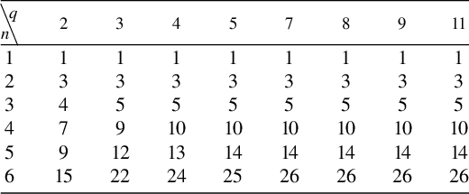
We now use Proposition 5.4 to study the number of isomorphism classes of unitary graphs in the family ${\mathbb {F}}_q[x]/f$ , where $f \in {\mathbb {F}}_q[x]$ and $\deg (f)=n.$ Table 1 shows this number for various values of n and q. As we can observe from this dataset, once we fix n, the number of isomorphism classes seems to stabilize when q gets bigger. In fact, we have the following proposition.

Table 1

The number of isomorphism classes of unitary graphs in the family ${\mathbb {F}}_q[x]/f$ , where $\deg (f)=n$ for various values of n and q.

Table 1 Long description

The table consists of a header row and six data rows. The header row lists the variable n in the first cell, followed by values of q: 2, 3, 4, 5, 7, 8, 9, and 11.

* Row 1: n equals 1. For all values of q from 2 to 11, the result is 1.

* Row 2: n equals 2. For all values of q from 2 to 11, the result is 3.

* Row 3: n equals 3. For q equals 2, the result is 4. For all other values of q from 3 to 11, the result is 5.

* Row 4: n equals 4. For q equals 2, the result is 7. For q equals 3, the result is 9. For all other values of q from 4 to 11, the result is 10.

* Row 5: n equals 5. For q equals 2, the result is 9. For q equals 3, the result is 12. For q equals 4, the result is 13. For all other values of q from 5 to 11, the result is 14.

* Row 6: n equals 6. For q equals 2, the result is 15. For q equals 3, the result is 22. For q equals 4, the result is 24. For q equals 5, the result is 25. For all other values of q from 7 to 11, the result is 26.

Proposition 5.5. Let n be a fixed number. Then, there exist constants $q_n, C_n$ depending only on n such that if $q \geq q_n$ , then the number of isomorphism classes of unitary graphs of the form $G_{f}(\{1 \})$ , where $f \in {\mathbb {F}}_q[x]$ and $\deg (f)=n$ , is exactly $C_n.$

To provide a proof for Proposition 5.5, we recall that for fixed $m,q$ , the number $S(m,q)$ of irreducible polynomials of degree m over ${\mathbb {F}}_q[x]$ is given by the following Gauss’s formula (see [Reference Chebolu and Mináč5] for a proof of this formula using the inclusion-exclusion principle):

(5-1) $$ \begin{align} S(m,q)=\frac{1}{m} \sum_{d \mid m} \mu(m/d)q^d. \end{align} $$

By (5-1), we see that for fixed n, $S(m,q)$ is asymptotically equivalent to $q^m/m$ for all $m \leq n.$ In particular, $S(m,q) \geq n$ for all q sufficiently large. We can now give a proof for Proposition 5.5.

Proof. Let $f \in {\mathbb {F}}_q[x]$ be a monic polynomial of degree n and let $(a_1, a_2, \ldots ,a_n)$ be its factorization type. Then,

$$ \begin{align*} \sum_{m=1}^n m a_m \leq n.\end{align*} $$

In particular, this shows that $a_m \leq n$ for all $1 \leq m \leq n.$ We can find a number $q_n$ such that for $q \geq q_n$ , we have $n \leq S(m,q)$ . Consequently, $a_m \leq S(m,q)$ as well. We then see that, as long as this condition is satisfied, there are sufficiently many irreducible polynomials of each degree m to realize every factorization type that occurs for a monic polynomial of degree n. Thus, the collection of possible factorization types is independent of q for all $q\ge q_n$ .

Remark 5.6. After the submission of this paper, we completed another paper studying the monotonicity of $S(m,q)$ with respect to both q and m; see [Reference Chebolu, Mináč, Nguyen and Tân6]. In particular, [Reference Chebolu, Mináč, Nguyen and Tân6, Theorem 5.5] shows that $ S(m,q)\geq S(1,q)=q$ unless $(m,q)=(2,2)$ . Therefore, in Proposition 5.5, we may take $q_n=n$ , as suggested by Table 1.

5.2 Isomorphic gcd-graphs

In the previous section, we discussed necessary and sufficient conditions for two unitary Cayley graphs to be isomorphic. In this section, we extend this further to the case of gcd-graphs. The case where f is a prime power is studied exclusively in Section 4, so we focus on the case where f has at least two distinct factors in this section. Since many of our insights arise from analyzing experimental data, we begin this section with a concrete numerical example.

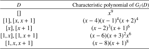
Example 5.7. Let $f= x(x+1) \in {\mathbb {F}}_3[x].$ Table 2 describes the isomorphism classes in the family of $G_{f}(D)$ , where D runs over the collection of subsets of ${\mathrm{Div}}(f)$ . We remark that we group these graphs by their characteristic polynomials; that is, by isospectral classes, but we have checked that elements in the same class are isomorphic as well. This is consistent with a conjecture of So for gcd-graphs over ${\mathbb {Z}}$ saying that two gcd-graphs $G_{f}(D_1)$ and $G_f(D_2)$ are isomorphic if and only if they are isospectral (see [Reference So20]).

Table 2

Isomorphism classes in the family $G_{f}(D)$ for $f=x(x+1)$ .

Table 2 Long description

The table consists of two columns. The first column is labeled D and the second column is labeled Characteristic polynomial of E sub z of D.

* Row 1: D is open bracket x close bracket. The characteristic polynomial is x to the 9 power.

* Row 2: D is open bracket 1 close bracket comma open bracket x comma x plus 1 close bracket. The characteristic polynomial is open parenthesis x minus 4 close parenthesis open parenthesis x minus 1 close parenthesis to the 4 power open parenthesis x plus 2 close parenthesis to the 4 power.

* Row 3: D is open bracket x close bracket comma open bracket x plus 1 close bracket. The characteristic polynomial is open parenthesis x minus 2 close parenthesis cubed open parenthesis x plus 1 close parenthesis to the 6th power.

* Row 4: D is open bracket 1 comma x close bracket comma open bracket 1 comma x plus 1 close bracket. The characteristic polynomial is open parenthesis x minus 6 close parenthesis open parenthesis x plus 3 close parenthesis squared x to the 6th power.

* Row 5: D is open bracket 1 comma x comma x plus 1 close bracket. The characteristic polynomial is open parenthesis x minus 8 close parenthesis open parenthesis x plus 1 close parenthesis to the 8th power.

Looking closely at the data, we have the following observation. While the isomorphism between $G_{f}(\{x\})$ and $G_{f}(\{x+1\})$ as well as the isomorphism between $G_{f}(\{1, x\})$ and $G_{f}(\{1, x+1\})$ are evident (via a substitution of variables), the isomorphism between $G_{f}(\{1\})$ and $G_{f}(\{x, x+1\})$ is less so. In fact, this isomorphism appears like a coincidence. More precisely, let us consider $f=x(x+1) \in {\mathbb {F}}_q[x]$ for a generic value of q. Then, the degree $G_{f}(\{1\})$ is $(q-1)^2$ and the degree of $G_{f}(\{x,x+1\}) = 2(q-1).$ These two degrees are equal only in the case $q=3.$

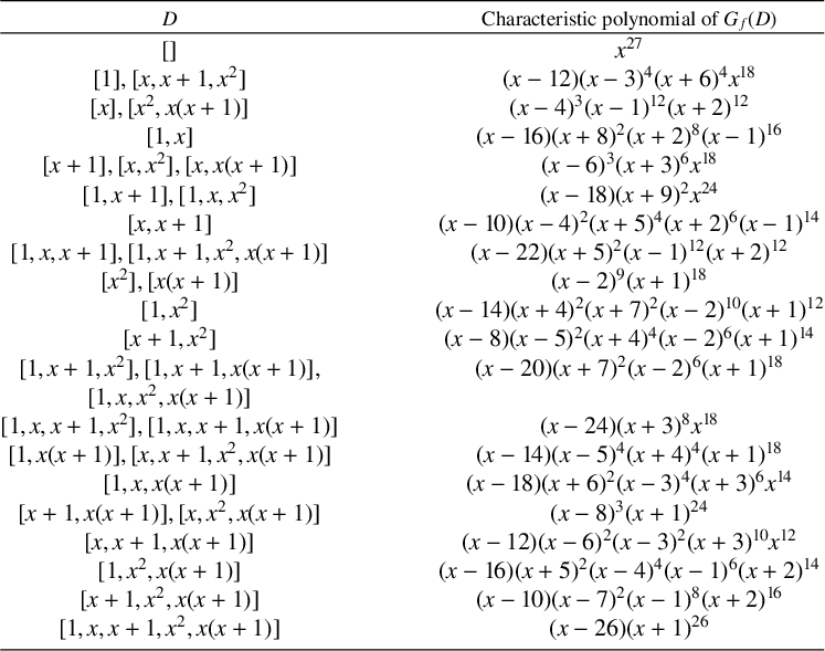
We discuss a more complicated example (see Table 3).

Example 5.8. Let $f = x^2(x+1) \in {\mathbb {F}}_3[x].$ As expected, there are more isomorphism classes in this family. We remark, however, that similar to the previous example, some isomorphisms depend on the fact that $q=3.$ More precisely, if we let ${f = x^2(x+1) \in {\mathbb {F}}_5[x]}$ , then we no longer have an isomorphism between the graphs ${G_{f}(\{1, x, x + 1\})}$ and ${G_{f}(\{1, x + 1, x^2, x (x + 1)\})}$ . However, some isomorphisms persist when we change q. For example, using the Python library NetworkX, we find the following two phenomena.

1. (1) For every $q \leq 5$ and $f = x^2(x+1) \in {\mathbb {F}}_q[x]$ , the two graphs $G_{f}(\{1,x,x^2\})$ and ${G_{f}(\{1, x+1\})}$ are isomorphic.

2. (2) For every $q \leq 5$ and $f= x^2(x+1) \in {\mathbb {F}}_q[x]$ , the graphs $G_{f}(\{1, x+1, x^2\})$ and $G_{f}(\{1, x+1, x(x+1)\})$ are also isomorphic.

Table 3

Isomorphism classes in the family $G_{f}(D)$ for $f=x^2(x+1) \in {\mathbb {F}}_3[x]$ .

Table 3 Long description

The table consists of 21 rows of data under two headers: D and Characteristic polynomial of E sub f open parenthesis D close parenthesis.

* Row 1: D is empty brackets [ ]. Polynomial is x super 27.

* Row 2: D is [ 1 ], [ x, x + 1, x super 2 ]. Polynomial is (x - 12)(x - 3) super 4 (x + 6) super 4 x super 18.

* Row 3: D is [ x ], [ x super 2, x(x + 1) ]. Polynomial is (x - 4) super 3 (x - 1) super 12 (x + 2) super 12.

* Row 4: D is [ 1, x ]. Polynomial is (x - 16)(x + 8) super 2 (x + 2) super 8 (x - 1) super 16.

* Row 5: D is [ x + 1 ], [ x, x super 2 ], [ x, x(x + 1) ]. Polynomial is (x - 6) super 3 (x + 3) super 6 x super 18.

* Row 6: D is [ 1, x + 1 ], [ 1, x, x super 2 ]. Polynomial is (x - 18)(x + 9) super 2 x super 24.

* Row 7: D is [ x, x + 1 ]. Polynomial is (x - 10)(x - 4) super 2 (x + 5) super 4 (x + 2) super 6 (x - 1) super 14.

* Row 8: D is [ 1, x, x + 1 ], [ 1, x + 1, x super 2, x(x + 1) ]. Polynomial is (x - 22)(x + 5) super 2 (x - 1) super 12 (x + 2) super 12.

* Row 9: D is [ x super 2 ], [ x(x + 1) ]. Polynomial is (x - 2) super 9 (x + 1) super 18.

* Row 10: D is [ 1, x super 2 ]. Polynomial is (x - 14)(x + 4) super 2 (x + 7) super 2 (x - 2) super 10 (x + 1) super 12.

* Row 11: D is [ x + 1, x super 2 ]. Polynomial is (x - 8)(x - 5) super 2 (x + 4) super 4 (x - 2) super 6 (x + 1) super 14.

* Row 12: D is [ 1, x + 1, x super 2 ], [ 1, x + 1, x(x + 1) ]. Polynomial is (x - 20)(x + 7) super 2 (x - 2) super 6 (x + 1) super 18.

* Row 13: D is [ 1, x, x super 2, x(x + 1) ]. Polynomial is blank.

* Row 14: D is [ 1, x, x + 1, x super 2 ], [ 1, x, x + 1, x(x + 1) ]. Polynomial is (x - 24)(x + 3) super 8 x super 18.

* Row 15: D is [ 1, x(x + 1) ], [ x, x + 1, x super 2, x(x + 1) ]. Polynomial is (x - 14)(x - 5) super 4 (x + 4) super 4 (x + 1) super 18.

* Row 16: D is [ 1, x, x(x + 1) ]. Polynomial is (x - 18)(x + 6) super 2 (x - 3) super 4 (x + 3) super 6 x super 14.

* Row 17: D is [ x + 1, x(x + 1) ], [ x, x super 2, x(x + 1) ]. Polynomial is (x - 8) super 3 (x + 1) super 24.

* Row 18: D is [ x, x + 1, x(x + 1) ]. Polynomial is (x - 12)(x - 6) super 2 (x - 3) super 2 (x + 3) super 10 x super 12.

* Row 19: D is [ 1, x super 2, x(x + 1) ]. Polynomial is (x - 16)(x + 5) super 2 (x - 4) super 4 (x - 1) super 6 (x + 2) super 14.

* Row 20: D is [ x + 1, x super 2, x(x + 1) ]. Polynomial is (x - 10)(x - 7) super 2 (x - 1) super 8 (x + 2) super 16.

* Row 21: D is [ 1, x, x + 1, x super 2, x(x + 1) ]. Polynomial is (x - 26)(x + 1) super 26.

We tried various other examples and found the following statement that explains the first phenomenon described in Example 5.8.

Proposition 5.9. Let $f = f_1 f_2$ , where $\gcd (f_1, f_2)=1.$ Assume further that $\mathrm {rad}(f_1)$ and $\mathrm {rad}(f_2)$ have the same factorization type. Let

$$ \begin{align*} D_1 = {\mathrm{Div}}(f_1), \quad D_2 = {\mathrm{Div}}(f_2) .\end{align*} $$

Then, $G_{f}(D_1)$ and $G_f(D_2)$ are isomorphic. In fact, they are both isomorphic to the wreath product $G_{{\mathbb {F}}_q[x]/\mathrm {rad}(f_1)}(\{1\}) * E_{m}$ , where $m= {|f|}/{|\mathrm {rad}(f_1)|}.$

Proof. By the Chinese remainder theorem,

$$ \begin{align*} R = {\mathbb{F}}_q[x]/(f_1f_2) \cong {\mathbb{F}}_q[x]/f_1 \times {\mathbb{F}}_q[x]/f_2.\end{align*} $$

Under this isomorphism and by the definition of $D_1$ , we can see that

$$ \begin{align*} (x_1, y_1), (x_2, y_2) \in {\mathbb{F}}_q[x]/f_1 \times {\mathbb{F}}_q[x]/f_2 \end{align*} $$

are adjacent in $G_{f}(D_1)$ if and only if $y_1-y_2 \in ({\mathbb {F}}_q[x]/f_2)^{\times }.$ We then see that $G_{f}(D_1)$ is isomorphic to the wreath product $G_{f_2}(\{1\}) * E_{m_1}$ , where $m_1=|f_1|.$ We remark that we can also get this isomorphism by observing that $f_2R$ is a homogeneous set in $G_{f}(D_1)$ and the required isomorphism follows from [Reference Mináč, Nguyen and Tân14, Theorem 5.5].

By the result from the previous section, we further have

$$ \begin{align*} G_{f_2}(\{1\}) \cong G_{\mathrm{rad}(f_2)}(\{1\}) * E_{m_2}, \end{align*} $$

where $m_2=|f_2|/|\mathrm {rad}(f_2)|.$ Since the wreath product is associative,

$$ \begin{align*} G_{f}(D_1) \cong G_{\mathrm{rad}(f_2)}(\{1\})* E_m ,\end{align*} $$

where $m= {|f|}/{|\mathrm {rad}(f_2)|}.$ An identical argument and the fact that $\mathrm {rad}(f_1), \mathrm {rad}(f_2)$ have the same factorization type show that $G_{f}(D_2)$ is isomorphic to $G_{\mathrm {rad}(f_1)}(\{1\}) * E_m$ as well. We conclude that $G_{f}(D_1) \cong G_f(D_2).$

Remark 5.10. We thank Professor Ki-Bong Nam for some discussion that led to the statement for Proposition 5.9. Specifically, Professor Nam suggested that we study generalized Euler numbers, which we now recall. Let A be a PID, $n \in A$ , and let m be a divisor of n. The generalized Euler number $\varphi _{m}(n)$ is the number of elements in the following set:

$$ \begin{align*} U_m(n) = \{ a \in A/n \mid \gcd(a,m) =1 \}.\end{align*} $$

When $m=n$ , $|U_m(n)|$ is precisely the Euler totient function of $n.$ In the setting of Proposition 5.9, $S_{D_1} = U_{f_2}(f_1f_2)$ , where $S_{D_1}$ is the generating set of the gcd-graph $G_{f}(D_1).$

We have the following corollary, which is a by-product of the proof for Proposition 5.9. We first introduce a standard notation. Suppose that g is an irreducible polynomial; we write $g^a \mid \mid f$ if $g^a \mid f$ , but $g^{a+1} \nmid f.$

Corollary 5.11. Let f be a polynomial. Suppose that f has distinct irreducible factors $f_1, f_2$ of the same degree. Let $a_1, a_2$ be two positive integers such that $f_1^{a_1} \mid \mid f$ and $f_2^{a_2} \mid \mid f.$ Let

$$ \begin{align*} D_1 = {\mathrm{Div}}(f_1^{a_1}) , \quad D_2 = {\mathrm{Div}}(f_2^{a_2}) .\end{align*} $$

Then, $G_{f}(D_1) \cong G_{f}(D_2).$

Proof. For $i \in \{1,2 \}$ , let $h_i=f/f_i^{a_i}$ . By the same argument as in the proof of Proposition 5.9 applied to $f = f_i^{a_i} h_i$ , we know that

$$ \begin{align*} G_{f}(D_i) \cong G_{\mathrm{rad}(h_i)}(\{1\}) * E_{|f/\mathrm{rad}(h_i)|}.\end{align*} $$

By definition, we know that $\mathrm {rad}(h_1)$ and $\mathrm {rad}(h_2)$ have the same factorization type. Furthermore, we also know that $|{\mathbb {F}}_q[x]/(f/\mathrm {rad}(h_1))|= |{\mathbb {F}}_q[x]/(f/\mathrm {rad}(h_2))|$ . Therefore, $G_{f}(D_1) \cong G_{f}(D_2).$

For the second phenomenon described in Example 5.8, we found the following generalization.

Proposition 5.12. Let $f_1, f_2$ be two distinct irreducible polynomials of the same degree. Let $n \geq 2$ be a positive integer, $f=f_1^nf_2$ ,

$$ \begin{align*} D_1 = \{1, f_2, f_1^2, \ldots, f_1^{n} \},\end{align*} $$

and

$$ \begin{align*} D_2 = \{1, f_2, f_1 f_2 \}.\end{align*} $$

Then, $G_{f}(D_1)$ and $G_{f}(D_2)$ are isomorphic.

Proof. By [Reference Mináč, Nguyen and Tân14, Theorem 5.5], the ideal $I_{f_1}$ generated by $f_1$ is a homogeneous set in $G_{f}(D_1)$ as well as $G_{f}(D_2).$ Furthermore,

$$ \begin{align*} G_{f}(D_1) \cong G_{f_1}(\{1\}) * G_{f_1^{n-1}f_2}(\{f_1, f_1^2, \ldots, f_1^{n-1}\}).\end{align*} $$

Similarly, we also have

$$ \begin{align*} G_{f}(D_2) \cong G_{f_1}(\{1\}) * G_{f_1^{n-1}f_2}(\{f_2\}).\end{align*} $$

Therefore, to complete the proof, we only need to show that

$$ \begin{align*} G_{f_1^{n-1}f_2}(\{f_1, f_1^2, \ldots, f_1^{n-1}\}) \cong G_{f_1^{n-1}f_2}(\{f_2\}) .\end{align*} $$

We observe that $G_{f_1^{n-1}f_2}(\{f_1, f_1^2, \ldots , f_1^{n-1}\})$ is isomorphic to $|f_1|$ disjoint copies of $G_{f_1^{n-2}f_2}(\{1, f_1, \ldots , f_1^{n-2}\})$ and $G_{f_1^{n-1}f_2}(\{f_2\})$ is isomorphic to $|f_2|$ disjoint copies of $G_{f_1^{n-1}}(\{1 \}).$ By Theorem 3.5 and the proof of Proposition 5.9,

$$ \begin{align*} G_{f_1^{n-2}f_2}(\{1, f_1, \ldots, f_1^{n-2}\}) \cong K_{|f_1|} * E_{|f_1|^{n-2}} \cong G_{f_1^{n-1}}(\{1 \}).\end{align*} $$

Summarizing all these isomorphisms, we conclude that $G_{f}(D_{1})$ and $G_{f}(D_{2})$ are isomorphic.

Remark 5.13. A by-product of the above proof is that if $f_1$ and $f_2$ are two distinct irreducible polynomials of the same degree, then for each $m \geq 1$ ,

$$ \begin{align*} G_{f_1^{m}f_2}(\{1, f_1, \ldots, f_1^{m}\}) \cong K_{|f_1|} * E_{|f_1|^{m}} \cong G_{f_1^{m+1}}(\{1 \}).\end{align*} $$

This isomorphism provides a simple construction of two isomorphic gcd-graphs with different moduli.

Remark 5.14. A conjecture of So [Reference So20, Conjecture 7.3] says that if n is an integer and $D_1, D_2$ are two distinct subsets of ${\mathrm{Div}}(n)$ , then the two gcd-graphs over ${\mathbb {Z}}$ , $G_n(D_1)$ and $G_n(D_2)$ , are not isomorphic.

As we have shown, this conjecture is not true if we consider gcd-graphs over ${\mathbb {F}}_q[x].$ We remark, however, that our constructions of isomorphic gcd-graphs of the form $G_{f}(D)$ , where f is fixed, are based on a crucial fact that f has two irreducible factors of the same degree. This could happen over ${\mathbb {F}}_q[x]$ but not over ${\mathbb {Z}}.$ As a result, we wonder whether So’s conjecture still holds for the family $G_{f}(D)$ under the additional assumption that irreducible factors of f have different degrees.