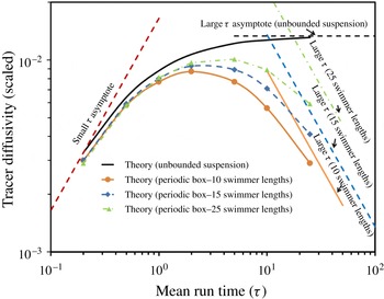
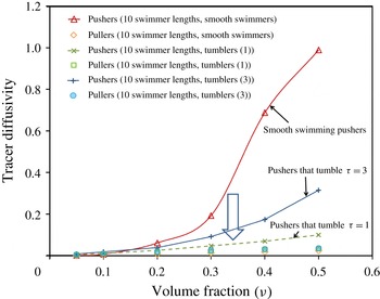
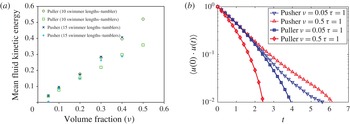
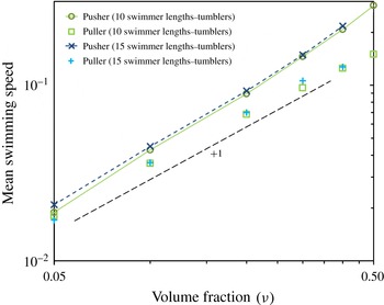
1. Introduction
The study of swimming microorgansims has, for a long time, been a fascinating field of research in fluid mechanics and transport phenomena. The early research in this field largely focused on the detailed swimming mechanism of single organisms, given the constraints imposed by a low Reynolds number fluid ambient (Gray & Hancock Reference Gray and Hancock1955; Gray Reference Gray1958; Brennen & Winet Reference Brennen and Winet1977; Purcell Reference Purcell1977). Single swimmer kinematics continues to be an area of interest (Lauga & Powers Reference Lauga and Powers2009). More recently, however, a great deal of interest has also been generated in this field due to observations of ‘collective behaviour’, especially in moderately concentrated suspensions of swimming bacteria. Experiments with suspensions of Escherichia coli (Wu & Libchaber Reference Wu and Libchaber2000) and Bacillus subtilis (Mendelson et al. Reference Mendelson, Bourque, Wilkening, Anderson and Watkins1999; Dombrowski et al. Reference Dombrowski, Cisneros, Chatkaew, Goldstein and Kessler2004; Sokolov et al. Reference Sokolov, Aranson, Kessler and Goldstein2007; Cisneros et al. Reference Cisneros, Kessler, Ganguly and Goldstein2011; Dunkel et al. Reference Dunkel, Heidenreich, Drescher, Wensink, Bär and Goldstein2013), for example, have revealed large scale fluid motions in the form of vortices and jets; the relevant scales being much larger than the size of individual organisms, although still smaller than those relevant to bio-convection (Hill & Pedley Reference Hill and Pedley2005). Other related observations include swimming speeds much greater than that of an isolated swimmer (Sokolov et al. Reference Sokolov, Aranson, Kessler and Goldstein2007), enhanced swimmer and tracer diffusivities (Wu & Libchaber Reference Wu and Libchaber2000; Soni et al. Reference Soni, Ali, Hatwalne and Shivashankar2003; Wu et al. Reference Wu, Roberts, Kim, Koch and DeLisa2006) and efficient fluid mixing (Sokolov et al. Reference Sokolov, Goldstein, Feldchtein and Aranson2009). A common feature of the above experiments is that they all involve rear-actuated swimmers or pushers. In contrast, Leptos et al. (Reference Leptos, Guasto, Gollub, Pesci and Goldstein2009) observed only a small increase in the diffusivities of colloidal tracer particles in a suspension of algae Chlamydomonas reinhardtii, a front-actuated swimmer or puller, that may be explained using scaling arguments based on binary tracer–algae interactions. This is consistent with theoretical predictions (discussed below) that suspensions of pushers are linearly unstable to coupled long-wavelength velocity and orientation perturbations, whereas suspensions of pullers are stable (Saintillan & Shelley Reference Saintillan and Shelley2007; Underhill, Hernandez-Ortiz & Graham Reference Underhill, Hernandez-Ortiz and Graham2008; Subramanian & Koch Reference Subramanian and Koch2009).
The role of long-ranged hydrodynamic interactions between swimmers in the collective behaviour in swimmer suspensions was first recognized by Simha & Ramaswamy (Reference Simha and Ramaswamy2002), who proposed continuum field equations for orientationally ordered swimmer suspensions with the individual swimmers modelled as force dipoles in light of the force-free constraint that applies to any athermal Stokesian swimmer. They showed that an initial state with either polar or nematic order is unstable to sufficiently long wavelength orientation perturbations. The stability of an isotropic base state, which is more relevant to bacterial suspensions at lower volume fractions, was analysed by Saintillan & Shelley (Reference Saintillan and Shelley2008a ), who found that this base state was unstable only for a suspension of slender pushers. That this hydrodynamic instability may underlie observations of collective motion has been confirmed via both particle-level simulations (Saintillan & Shelley Reference Saintillan and Shelley2007; Underhill et al. Reference Underhill, Hernandez-Ortiz and Graham2008; Saintillan & Shelley Reference Saintillan and Shelley2012) and simulations of the continuum field equations (Saintillan & Shelley Reference Saintillan and Shelley2008b ). The swimmers in these simulations change their orientations due to hydrodynamic and steric (short-range repulsive) interactions with other swimmers, although only the former are relevant for the volume fractions under consideration. None of the above efforts consider the effects of intrinsic orientation decorrelation mechanisms, however, and these are a key feature of bacterial motion on the micro-scale. For example, an isolated bacterium such as an E. coli executes a run-and-tumble motion where it swims in a directed sense for a certain amount of time (a run), and this is followed by a sharp change in orientation termed a tumble (Berg Reference Berg1993, Reference Berg2004). Even during a run, the bacterium deviates from a straight path due to imperfections in the flagellar bundle, and the resulting small-amplitude orientation fluctuations, resemble a rotary diffusion process (Berg Reference Berg1993; Koch & Subramanian Reference Koch and Subramanian2011). The run-and-tumble motility paradigm applies to other micro-scale swimmers including other bacteria, both uniflagellated (C. crescentus; Liu et al. Reference Liu, Gulino, Morse, Tang, Powers and Breuer2014) and peritrichously flagellated (B. subtilis; Rao, Kirby & Arkin Reference Rao, Kirby and Arkin2004, S. typhimurium; Stocker Reference Stocker2011) ones, and eukaryotes (C. reinhardtii; Polin et al. Reference Polin, Tuval, Drescher, Gollub and Goldstein2009), although the underlying mechanisms for the tumble events are varied. In what follows, swimmers which lack any intrinsic orientation relaxation mechanisms, and only change their orientation due to hydrodynamic interactions, as in the simulations quoted above, are termed straight swimmers. In this work, we present the first particle-based simulations of a suspension of hydrodynamically interacting swimmers with intrinsic orientation relaxation mechanisms.
One of the motivations for the current work is that consideration of only straight swimmers, as in earlier efforts (Saintillan & Shelley Reference Saintillan and Shelley2007; Underhill et al.
Reference Underhill, Hernandez-Ortiz and Graham2008; Saintillan & Shelley Reference Saintillan and Shelley2008b
, Reference Saintillan and Shelley2012), leads to an unbounded suspension of pushers being unstable at any non-zero concentration. Experiments with bacterial suspensions, however, report the onset of collective motion only above a finite concentration threshold (Wu et al.
Reference Wu, Roberts, Kim, Koch and DeLisa2006; Sokolov et al.
Reference Sokolov, Aranson, Kessler and Goldstein2007, Reference Sokolov, Goldstein, Feldchtein and Aranson2009; Sokolov & Aranson Reference Sokolov and Aranson2012); for instance, Sokolov & Aranson (Reference Sokolov and Aranson2012) report the threshold for collective motion corresponding to a B. subtilis concentration of approximately
 $10^{10}~\text{cm}^{-3}$
. Subramanian & Koch (Reference Subramanian and Koch2009) were the first to analyse a suspension of bacteria that that execute a run-and-tumble motion, via a long-wavelength linear stability analysis. They derived a critical value for the swimmer concentration beyond which the instability sets in which depends on only the intrinsic swimming parameters (the swimmer length
 $L$
, the swimming speed in isolation
 $U$
, the average tumble frequency
 ${\it\tau}^{-1}$
and the rotary diffusivity during a run
 $D_{r}$
). The critical hydrodynamic volume fraction for a suspension of tumblers is given by:
 $$\begin{eqnarray}nL^{3}|_{crit}=\frac{\displaystyle \frac{5}{C\mathscr{F}({\it\gamma})}\left(\frac{L}{U{\it\tau}}\right)}{\displaystyle \left(1-\frac{5\mathscr{G}({\it\gamma})}{2C\mathscr{F}({\it\gamma})}\left(\frac{L}{U{\it\tau}}\right)\right)},\end{eqnarray}$$
and, for a suspension of rotary diffusers, the threshold is given by:
 $$\begin{eqnarray}nL^{3}|_{crit}=\frac{\displaystyle \frac{30}{C\mathscr{F}({\it\gamma})}\left(\frac{D_{r}L}{U}\right)}{\displaystyle \left(1-\frac{15\mathscr{G}({\it\gamma})}{C\mathscr{F}({\it\gamma})}\left(\frac{D_{r}L}{U}\right)\right)}.\end{eqnarray}$$
The general expression, when tumbling and rotary diffusion act together, may be obtained by using
 $({\it\tau}^{-1}+6D_{r})$
as the effective rate of relaxation instead of
 ${\it\tau}^{-1}$
in (1.1). In the above equations,
 $C$
is a constant characterizing the intrinsic swimming dipole,
 $\mathscr{F}({\it\gamma})$
is a dimensionless function of the aspect ratio
 ${\it\gamma}$
that characterizes the rotation of the swimmer in a linear flow and
 $\mathscr{G}({\it\gamma})$
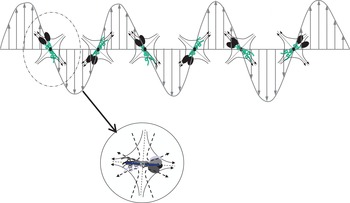
is related to the induced dipole arising from the bacterium inextensibility. The physical mechanism underlying the instability is shown in figure 1. An anisotropy in the swimmer orientation distribution, in response to a long wavelength velocity perturbation, leads to the intrinsic force dipoles driving a flow that reinforces the original perturbation. The instability arises thus from the mutual reinforcement of long-wavelength orientation and velocity fluctuations. In the limit of long wavelengths, the response of the orientation anisotropy to the local shearing perturbation may be interpreted in terms of a negative contribution to the effective shear viscosity (Hatwalne et al.
Reference Hatwalne, Ramaswamy, Rao and Simha2004; Subramanian & Koch Reference Subramanian and Koch2009). An instability sets in when the sum of the solvent and bacterial contributions to the shear viscosity equals zero. The reduction in shear viscosity, in the stable regime, has been confirmed by experiments (Sokolov & Aranson Reference Sokolov and Aranson2009; Gachelin et al.
Reference Gachelin, Miño, Berthet, Lindner, Rousselet and Clément2013).
Physical mechanism of instability in a suspension of pushers, illustrating coupled orientation and velocity fluctuations. The inset highlights the alignment of the slender swimmers along the local extensional axis.

For the simulations in this paper,
 $\mathscr{F}({\it\gamma})=1$
, since we consider the swimmers to be slender rods for which
 ${\it\gamma}\rightarrow \infty$
. Further,
 $\mathscr{G}({\it\gamma})$
is zero since we neglect the effects of the induced dipole in our simulations. Thus, the threshold for a suspension of tumblers relevant to the present simulations is given by:
 $$\begin{eqnarray}nL^{3}|_{crit}=\frac{5}{C}\left(\frac{L}{U{\it\tau}}\right),\end{eqnarray}$$
and that for a suspension of rotary diffusers is given by:
 $$\begin{eqnarray}nL^{3}|_{crit}=\frac{30}{C}\left(\frac{LD_{r}}{U}\right).\end{eqnarray}$$
From (1.3) and (1.4), we see that in the dilute limit, the non-dimensional parameter characterizing the instability is
 $nUL^{2}{\it\tau}$
for tumblers, and
 $nUL^{2}/D_{r}$
for rotary diffusers. It is important to note that there remains a sensible theoretical prediction for the stability of a swimmer suspension to compare to, even with the neglect of induced stresses. The aforementioned stability thresholds vanish in the limiting case of straight swimmers (
 ${\it\tau},D_{r}^{-1}\rightarrow \infty$
), implying that a suspension of such swimmers is always unstable, as mentioned above. The confirmation of the above results using computations should serve as a valuable guide for experiments which can sweep through a sequence of volume fractions or mean-run-times (
 ${\it\tau}$
) to detect the onset of collective behaviour. The volume fraction and swimming speeds have been varied in earlier experiments (Sokolov & Aranson Reference Sokolov and Aranson2009, Reference Sokolov and Aranson2012), while the experimental realization of different values of the mean-run-time has been shown to be possible by tailoring different mutant strains of E. coli (Karmakar et al.
Reference Karmakar, Gulvady, Tirumkudulu and Venkatesh2014).
Apart from the long-wavelength analysis of Subramanian & Koch (Reference Subramanian and Koch2009) for run-and-tumble bacteria, the complete (discrete) spectrum has been analysed by Saintillan & Shelley (Reference Saintillan and Shelley2008b
) for straight swimmers, by Subramanian, Koch & Fitzgibbon (Reference Subramanian, Koch and Fitzgibbon2011) for random tumblers (also see Subramanian & Nott Reference Subramanian and Nott2012), and by Hohenegger & Shelley (Reference Hohenegger and Shelley2010) for rotary diffusers. The main result for straight swimmers is that, for any swimmer volume fraction, there exists a critical wavenumber below which there are unstable (growing) modes and it is given by
 $k_{m}^{\prime }=0.09CnL^{2}$
. In simulations, however, the size of the simulation box imposes a restriction on the maximum wavelength (or minimum wavenumber) of the perturbation. Thus, for small enough box sizes and swimmer concentrations, the minimum unstable wavenumber will be greater than the critical wavenumber
 $k_{m}^{\prime }$
(which scales as
 $O(nL^{3})^{-1}$
), implying that the suspension will be artificially stabilized by the imposed periodicity. An estimate of the finite critical concentration above which a periodic suspension is unstable may be calculated by equating the critical wavenumber
 $k_{m}^{\prime }$
with the inverse box size, which can in turn be rearranged to give the critical volume fraction as:
 $$\begin{eqnarray}\displaystyle n_{crit}\left(\frac{L}{2}\right)^{3}={\it\nu}_{crit}=\frac{1}{0.72C}\frac{L}{L_{box}}, & & \displaystyle\end{eqnarray}$$
where we have used
 $L/2$
to define the volume fraction to ensure consistency with earlier efforts (Saintillan & Shelley Reference Saintillan and Shelley2007, Reference Saintillan and Shelley2012). The unbounded suspension result of
 ${\it\nu}_{crit}=0$
is recovered by letting
 $L/L_{box}\rightarrow 0$
. It must be noted that even in simulations of straight swimmers, the swimmers inevitably undergo orientation decorrelation due to hydrodynamic interactions. However, for large aspect ratios, as shown by Subramanian & Koch (Reference Subramanian and Koch2009), the rate of orientation decorrelation, as characterized by a hydrodynamic rotary diffusivity, is too weak to stabilize the suspension. This then leads to the aforementioned unconditional instability of a suspension of slender-bodied straight swimmers.
A common feature of the above theoretical efforts is the assumption of diluteness (
 $nL^{3}\ll 1$
) so that pair (and higher order) correlations between swimmers may be neglected. Each swimmer only sees the effects of others as an imposed mean field. Particle-level simulations are therefore necessary to test the validity of the continuum theories, and more importantly, to study the dynamics in swimmer suspensions at higher concentrations when
 $nL^{3}\sim O(1)$
. Indeed, the experimentally observed threshold number density of
 $O(10^{10}~\text{cm}^{-3})$
(Sokolov & Aranson Reference Sokolov and Aranson2012), mentioned earlier, corresponds to
 $nL^{3}\sim 10$
(accounting for the total B. subtilis length of
 $O(10~{\rm\mu}\text{m})$
), when the dilute regime theory may no longer be quantitatively valid. Additionally, simulations allow us easier control of certain parameters than experiments, especially since the experimental preparation of swimmer suspensions, with parameters in a narrow range, remains a delicate task. Earlier simulation efforts concerning straight-swimmer suspensions, with a rigorous treatment of hydrodynamic interactions, cover a range of geometries and models for the actuation.
Hernandez-Ortiz, Stoltz & Graham (Reference Hernandez-Ortiz, Stoltz and Graham2005) first proposed a dumbbell model for force-free swimmers consisting of point forces (beads) connected by an inextensible rod, with actuation applied to one of the beads. At large length scales, such swimmers interact via dipolar velocity fields. However, the singular near field associated with the point dipole led to erroneously enhanced swimmer diffusivities at higher volume fractions. Using regularized dipoles instead, Underhill et al. (Reference Underhill, Hernandez-Ortiz and Graham2008) later simulated both pusher and puller suspensions in a spatially periodic setting. For pushers, the diffusivity of non-Brownian tracer particles was found to increase with the simulation domain size; the tracer diffusivities were seen to be much smaller for pullers. The large magnitudes and the box-size-dependence of tracer diffusivities in pusher suspensions are consistent with the notion of a linear instability (Saintillan & Shelley Reference Saintillan and Shelley2008b ; Subramanian & Koch Reference Subramanian and Koch2009). A drawback of the regularized dipole model is that many of the predictions end up depending on the length scale of regularization.
The above unattractive feature can be eliminated by considering large-aspect-ratio swimmers with interactions governed by viscous slender-body theory. Such slender swimmer models were considered by Saintillan & Shelley (Reference Saintillan and Shelley2007), who simulated a suspension of self-propelled rods with a specified tangential stress that causes a rod to swim in either a pusher or puller configuration. In addition to confirming the instability of an initial orientationally ordered state, Saintillan & Shelley (Reference Saintillan and Shelley2007) found that the saturated state for pushers and pullers, resulting from the instability, showed very different local order, with neighbouring pairs of pushers and pullers preferring parallel and anti-parallel alignment, respectively. Interestingly, even in the unstable regime, the swimmer translational diffusivity was seen to be well approximated by
 $U^{2}/(6D_{r})$
, obtained from Taylor dispersion theory,
 $D_{r}^{-1}$
here being the decorrelation time due to hydrodynamic interactions. Swimmer transport is thus primarily governed by the swimming motion along with orientation decorrelations and is not a reliable indicator of an instability. More recently, Saintillan & Shelley (Reference Saintillan and Shelley2012) have presented a detailed simulation study of straight swimmers contrasting pushers and pullers. They identified several features of the instability for pushers such as enhanced swimming speeds, fluid velocity fluctuations, fluid mixing and enhanced tracer diffusivities. The tracer diffusivity was found to be a sensitive measure of the onset of collective motion.
Pedley and co-workers have studied the dynamics and rheology of suspensions of spherical squirmers (Ishikawa, Locsei & Pedley Reference Ishikawa, Locsei and Pedley2008; Ishikawa & Pedley Reference Ishikawa and Pedley2008) via an extension of the original Stokesian dynamics algorithm (Brady & Bossis Reference Brady and Bossis1988). Squirmers swim due to a specified surface tangential velocity and may be accurate models for P. caudatum and Volvox which swim by waving hair-like projections on their surface (cilia for P. caudatum and outward facing flagella in case of Volvox). The squirmers simulated have a surface velocity that corresponds to a dipole–quadrupole combination at their centres, the dipole again being contractile or extensile in character. The spherical shape, however, makes the behaviour of squirmers very different from the slender swimmers discussed above since there is no means of inducing an orientational anisotropy by virtue of an imposed extensional flow. In contrast to the studies above, squirmers show interesting behaviour for the case of pullers. There is a local ordering with neighbouring pullers swimming parallel to one another (Ishikawa et al. Reference Ishikawa, Locsei and Pedley2008), and recent work has found a globally ordered polar phase of spherical squirmers (pullers) driven solely by hydrodynamic interactions (Evans et al. Reference Evans, Ishikawa, Yamaguchi and Lauga2011). These features are opposite to the anti-parallel orientation of nearby pairs seen for rod-like pullers in simulations by Saintillan & Shelley (Reference Saintillan and Shelley2007). Further, as indicated above, the swimmer suspension instability is crucially related to a decrease in the zero shear viscosity, with increasing volume fraction, of a dilute suspension of anisotropic pushers. However, a reduction in viscosity of a squirmer suspension is only observed in a gravitational field (Ishikawa & Pedley Reference Ishikawa and Pedley2007). Another work dealing with spherical swimmers is by Mehandia & Nott (Reference Mehandia and Nott2008), who used Stokesian dynamics to model a monolayer of hydrodynamically interacting spherical swimmers. A more detailed discussion of these efforts may be found in the reviews by Koch & Subramanian (Reference Koch and Subramanian2011) and Subramanian & Nott (Reference Subramanian and Nott2012).
Our aim here is to study the effects of intrinsic decorrelation mechanisms on the swimmer suspension dynamics and estimate (numerically) a threshold for the onset of instability in a pusher suspension which is solely a function of the intrinsic swimming parameters, and unlike (1.5), is independent of the simulation box size. The rest of the paper is organized as follows. In § 2, we present a detailed account of the simulation methodology. Starting from our model for the individual swimmers, we move on to describing our approach for calculating the hydrodynamic interactions between them in a spatially periodic setting. We use simplifying assumptions which lead to a kinematic particle-level simulation with substantial savings in computational effort, allowing us to explore large simulation box sizes. Our largest simulations involve over 25 000 swimmers in a 40-swimmer-length box, corresponding to a hydrodynamic volume fraction of
 $N(L/2L_{box})^{3}=0.05$
, where
 $N$
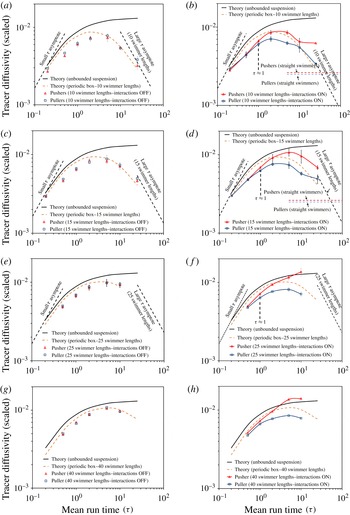
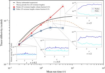
is the number of swimmers. We also describe the modelling approaches used for tumbling and rotary diffusion in this section, and validate these by comparison with theory. In § 3, we validate our kinematic simulation methodology by performing simulations of straight slender swimmers, and comparing our results with earlier simulations of such swimmers by Saintillan & Shelley (Reference Saintillan and Shelley2007, Reference Saintillan and Shelley2012), and with the simulations of regularized dipole swimmers by Underhill et al. (Reference Underhill, Hernandez-Ortiz and Graham2008). Next, in § 4, we study suspensions of swimmers which tumble and rotary diffuse in addition to interacting hydrodynamically with other swimmers. In § 4.1 we develop an analytical expression for the tracer diffusivity in a spatially periodic swimmer suspension of tumblers. Periodicity leads to a non-monotonic dependence of the predicted tracer diffusivity on the orientation relaxation time, a feature reproduced in our simulations that lie in the stable regime. While the non-monotonicity is a crucial feature of our simulations involving weakly interacting slender swimmers at dilute volume fractions, in general, the degree of non-monotonicity depends on the strength of hydrodynamic interactions; it is shown that the tracer diffusivity transitions to a nearly monotonic behaviour when the hydrodynamic orientation decorrelation time becomes comparable to or smaller than the time required for a swimmer to traverse the simulation box. A key aspect of the periodic-box theory is that the tracer diffusivities are identical for both pusher and puller suspensions in the dilute regime, and this allows one to detect the onset of instability in the simulations as a bifurcation in the tracer diffusivity curves with the pusher diffusivities being larger beyond the threshold. We show, through our simulations in §§ 4.2 and 4.3, that the threshold for the onset of collective motion depends on both the suspension concentration and rate of intrinsic orientation decorrelation. Consistent with theory, the dimensionless parameters
 $nUL^{2}{\it\tau}$
and
 $nUL^{2}/D_{r}$
control the stability threshold in suspensions of tumblers and rotary diffusers, respectively. The numerical estimates for the box-size-independent thresholds obtained from our simulations however fall consistently below the theoretical predictions. In § 5, we present a summary of the main results, and comment on future extensions.
2. Simulation method
We consider rod-like swimmers which operate at low Reynolds numbers, and hence, are force-free at all times. The passive portions of such a swimmer drag the fluid along as it swims, while the propulsive parts push fluid in the opposite direction. Therefore, the disturbance velocity due to a swimmer is dipole-like at long distances, and decays as
 $1/r^{2}$
, where
 $r$
is the distance from the swimmer. Importantly, the divergence of the disturbance velocity in the near field (scales much smaller than
 $L$
) is weaker, being
 $O(\log r)$
, which eliminates the dependence on the regularization length scale, a feature of the force dipoles simulated by Graham and co-workers (Underhill et al.
Reference Underhill, Hernandez-Ortiz and Graham2008). Since the collective behaviour we are interested in studying is solely attributed to the intrinsic stresses that arise due to swimming in isolation, we neglect the induced stresses that arise due to the swimmer inextensibility. The intrinsic stress can be specified a priori based only on the isolated swimming parameters, and as a result, the swimmer disturbance fields are known beforehand. One only has to now convect and rotate each slender swimmer in a known ambient (due to all other swimmers), and in a manner consistent with viscous slender-body theory (Batchelor Reference Batchelor1970). This makes our simulations kinematic in nature since the translational and angular velocities of the swimmers can be calculated explicitly, at each instant in time, as a function of the swimmer configurations. Our interest in studying the threshold for collective motion in a swimmer suspension motivates us to study two types of swimmers, namely, pushers and pullers, described in the following section.
2.1. Single swimmer model
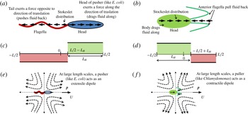
Micro-scale swimmers such as E. coli and Chlamydomonas use flagella, whip-like attachments to the cell body, to swim in a viscous fluid ambient. They differ in their swimming mechanism, however, and are classified as pushers and pullers, respectively. Pushers have a propulsive part (the posterior flagellar bundle in E. coli) which pushes the head of the organism through the fluid, leading to an extensile intrinsic dipole (see figure 2
a). Pullers have the propulsive portion (the pair of anterior flagella in Chlamydomonas) pulling the head through the fluid with the aid of a breast-stroke-like motion, leading to a contractile dipole (see figure 2
b). Typical pushers and puller velocity fields are shown in figure 2(e,f). We model these swimmers as (infinitely) slender rods which, given the large aspect ratios of typical pushers (
 ${\sim}6$
for E. coli), is a fairly good approximation. The intrinsic force distribution is taken to be a line distribution of Stokeslets (Leal Reference Leal2007) with the Stokeslets being parallel (anti-parallel) to the swimming direction on the passive (propulsive) portion. The distribution is parameterized by
 ${\it\alpha}_{1}=L_{H}/L$
, where
 $L_{H}$
and
 $L$
are the head and total swimmer lengths, and is of the form
 $f(s)\boldsymbol{p}$
, with:
 $$\begin{eqnarray}f(s)=\left\{\begin{array}{@{}ll@{}}\displaystyle \frac{-F_{D}}{(1-{\it\alpha}_{1})L}\quad & \text{for }-L/2<s<L(1/2-{\it\alpha}_{1}),\\ \displaystyle \frac{F_{D}}{{\it\alpha}_{1}L}\quad & \text{for }L(1/2-{\it\alpha}_{1})<s<L/2,\end{array}\right.\end{eqnarray}$$
for pushers, where
 $F_{D}$
is the drag force on the head. Here,
 $\boldsymbol{p}$
denotes the swimmer orientation, and
 $s$
is the coordinate along the swimmer axis measured from the centre (see figure 2
c,d). The model above does not aim to elucidate the actual swimming mechanism, but merely assumes one to exist and that it leads to a non-trivial swimming velocity and force distribution. Thus, features of the velocity field specific to a given propulsion mechanism are neglected. For instance, in E. coli, the counter-rotation of the head and the propelling flagellar bundle leads to an additional torque dipole or a vortlet singularity (Ghose & Adhikari Reference Ghose and Adhikari2014), and the associated
 $O(1/r^{3})$
velocity field is neglected here (a reasonable approximation for slender swimmers since the singularity strength must scale with the much smaller head diameter). The puller model is the same as (2.1), but with the force distribution reversed. Again, our intention in modelling pullers is not to describe specific organisms such as Chlamydomonas, whose near-field velocity may be complicated by unsteady stroke kinematics and the presence of closed streamlines (Guasto, Johnson & Gollub Reference Guasto, Johnson and Gollub2010; Drescher et al.
Reference Drescher, Dunkel, Cisneros, Ganguly and Goldstein2011), but to study the effect of the contractile nature of the dipole on collective motion. The main role for the puller simulations is to serve as a baseline for contrast.
Schematic of the single swimmer model. (a,b) depict the Stokeslet distribution used to model a pusher and puller, respectively. The corresponding variations of the linear force density along the swimmer axis are shown in (c,d). (e,f) Show the dipole velocity field at large length scales; the dipole has an extensile character for the pusher and is contractile in nature for the puller.

The results presented here are for fore–aft symmetric swimmers
 $({\it\alpha}_{1}=1/2)$
with a Heaviside force density profile. The value of
 $F_{D}$
in (2.1) is obtained from equating the drag on a spheroidal E. coli head to that on a slender rod moving with the same speed. This leads to an aspect ratio of
 $6$
for the fore–aft symmetric swimmers simulated. Changes in
 ${\it\alpha}_{1}$
do not qualitatively alter the results. We have also considered a sinusoidally varying force density, and again find no qualitative differences.
2.2. Hydrodynamic interactions in a swimmer suspension
The swimmers, as they swim along, ‘stir’ the suspending fluid, and thereby, affect the motion of other swimmers. In the low Reynolds number regime, relevant to most micro-scale swimmers (for E. coli,
 $L\approx 12~{\rm\mu}\text{m}$
and
 $U\approx 10~{\rm\mu}\text{m}~\text{s}^{-1}$
, so that the Reynolds number,
 $Re={\it\rho}UL/{\it\eta}$
, is
 $O(10^{-4})$
for swimming in an aqueous medium. The
 $Re$
’s characterizing the coherent structures, such as the vortices and jets, that dominate the collective dynamics, continues to remain small (Tuval et al.
Reference Tuval, Cisneros, Dombrowski, Wolgemuth, Kessler and Goldstein2005)), the governing equations are the Stokes equations with an additional forcing term due to the swimmers and the continuity equation for an incompressible fluid. This set of equations, in dimensionless form, can be written as:
 $$\begin{eqnarray}\displaystyle & \displaystyle -\boldsymbol{{\rm\nabla}}p+{\rm\nabla}^{2}\boldsymbol{u}=\unicode[STIX]{x1D63D}, & \displaystyle\end{eqnarray}$$
 $$\begin{eqnarray}\displaystyle & \displaystyle \boldsymbol{{\rm\nabla}}\boldsymbol{\cdot }\boldsymbol{u}=0, & \displaystyle\end{eqnarray}$$
 $p$
and
 $\boldsymbol{u}$
are the pressure and velocity fields, and
 $$\begin{eqnarray}\unicode[STIX]{x1D63D}=-\mathop{\sum }_{m=1}^{\infty }\int _{-1}^{1}{\it\delta}(\boldsymbol{x}-\boldsymbol{x}_{m}-\boldsymbol{p}_{m}s)f(s)\boldsymbol{p}_{m}\,\text{d}s,\end{eqnarray}$$
is the forcing term due to the suspended swimmers. Here,
 $\boldsymbol{x}_{m}$
and
 $\boldsymbol{p}_{m}$
are the position and orientation of the
 $m$
th swimmer. We have used the following scales for non-dimensionalization: the length scale is
 $l_{c}=L/2$
; the time scale is
 $t_{c}=L/(2U)$
; and forces are scaled by
 $F_{c}={\it\mu}UL/2$
. Henceforth, we will be using dimensionless variables with the same notation as before. In dimensionless terms, the swimmer length is
 $2$
and its isolated swimming speed is unity.
The simulation domain is a cubic unit cell of side length
 $L_{box}$
having
 $N$
swimmers with centres at
 $\boldsymbol{x}_{1},\boldsymbol{x}_{2},\ldots ,\boldsymbol{x}_{N}$
, and with orientations
 $\boldsymbol{p}_{1},\boldsymbol{p}_{2},\ldots ,\boldsymbol{p}_{N}$
, supplemented by periodic boundary conditions. With this arrangement, the summation term in (2.4) can be written:
 $$\begin{eqnarray}\unicode[STIX]{x1D63D}=-\mathop{\sum }_{\boldsymbol{l}}\mathop{\sum }_{i=1}^{N}\int _{-1}^{1}{\it\delta}(\boldsymbol{x}-\boldsymbol{x}_{i}-\hat{\boldsymbol{p}}_{i}s-\boldsymbol{l})f(s)\boldsymbol{p}_{i}\,\text{d}s,\end{eqnarray}$$
where the inner summation denotes a sum over the simulation box (
 $\boldsymbol{l}=0$
), and the outer summation involving the lattice vector
 $\boldsymbol{l}$
is over the periodic images. For numerical purposes, the swimmer line force distribution is specified using point forces at discrete points along the swimmer axis and the integrals involving the force distribution are computed using Gaussian quadrature. With each swimmer being discretized as
 $M$
quadrature points, (2.5) can be written as:
 $$\begin{eqnarray}\unicode[STIX]{x1D63D}=-\mathop{\sum }_{\boldsymbol{l}}\mathop{\sum }_{i=1}^{N}\boldsymbol{p}_{i}\mathop{\sum }_{j=1}^{M}{\it\delta}(\boldsymbol{x}-\boldsymbol{x}_{i}-\boldsymbol{p}_{i}s_{j}-\boldsymbol{l})w_{j}\,f(s_{j}),\end{eqnarray}$$
where
 $f(s_{j})\boldsymbol{p}_{i}$
is the
 $j$
th Stokeslet on the
 $i$
th swimmer in the simulation box, and the
 $w_{j}$
’s are the quadrature weights. Absorbing the quadrature weights into the force density (Saintillan, Darve & Shaqfeh Reference Saintillan, Darve and Shaqfeh2005), the momentum equation, using (2.6), is given by:
 $$\begin{eqnarray}\displaystyle -\boldsymbol{{\rm\nabla}}p+{\rm\nabla}^{2}\boldsymbol{u}=-\mathop{\sum }_{\boldsymbol{l}}\mathop{\sum }_{i=1}^{N}\boldsymbol{p}_{i}\mathop{\sum }_{j=1}^{M}{\it\delta}(\boldsymbol{x}-\boldsymbol{x}_{i}-\boldsymbol{p}_{i}s_{j}-\boldsymbol{l})f(s_{j}). & & \displaystyle\end{eqnarray}$$
One has to, in effect, solve the Stokes equations for
 $N\times M$
interlacing simple cubic arrays of point forces. A solution for a single simple cubic array of point forces was first derived by Hasimoto (Reference Hasimoto1959). Hasimoto’s approach has been extended to the case of interlacing arrays in the context of simulating suspensions of slender fibres (Mackaplow & Shaqfeh Reference Mackaplow and Shaqfeh1998; Butler & Shaqfeh Reference Butler and Shaqfeh2002). Using a different approach, interlacing cubic arrays of finite-sized spheres corresponding to a random array in the original unit cell were analysed by Beenakker (Reference Beenakker1986), and this alternate approach has been adopted by Brady and co-workers in their Stokesian dynamics algorithm (Brady & Bossis Reference Brady and Bossis1988; Brady et al.
Reference Brady, Phillips, Lester and Bossis1988). These two approaches are, of course, equivalent (Krishnamurthy Reference Krishnamurthy2014), and we follow Hasimoto (Reference Hasimoto1959).
As indicated above, the derivation of the disturbance velocity field in an infinite spatially periodic swimmer suspension, accounting for the re-normalization of the long-ranged hydrodynamic interactions, is now standard and follows the literature for passive suspensions (Brady et al.
Reference Brady, Phillips, Lester and Bossis1988). Briefly, the velocity and pressure gradients are expanded in a Fourier series with the
 $\boldsymbol{k}=0$
terms being excluded due to the total force per unit cell being balanced by a mean pressure gradient. From a numerical point of view, one needs to exclude the
 $\boldsymbol{k}=0$
terms even for a suspension of force-free swimmers (these terms correspond to a specification of the particle stress in a homogeneous isotropic swimmer suspension). Once the
 $\boldsymbol{k}=0$
terms are interpreted correctly, an exact periodic solution to the Stokes equations, in terms of a slowly convergent series in wavenumber space, results. This series is only conditionally convergent at large
 $k$
, reflecting the fact that the Fourier transforms of the physical space singularities (force-multipoles) must be interpreted as generalized functions. The slow convergence in
 $k$
is resolved in the usual manner by using the Ewald summation technique (Ewald Reference Ewald1921; Hasimoto Reference Hasimoto1959; Beenakker Reference Beenakker1986), which involves splitting the original sum into real and Fourier space sums, with a cutoff parameter or Ewald coefficient,
 ${\it\alpha}$
, tuned such that the total cost of the computation is minimized. The final result for the disturbance velocity in terms of the real and Fourier sums is:
 $$\begin{eqnarray}\displaystyle \boldsymbol{u}(\boldsymbol{x}) & = & \displaystyle \frac{1}{4{\rm\pi}}\left[\mathop{\sum }_{\boldsymbol{l}}\mathop{\sum }_{i=1}^{N}\mathop{\sum }_{j=1}^{M}\unicode[STIX]{x1D63C}({\it\alpha},\boldsymbol{x}-\boldsymbol{x}_{i}-\boldsymbol{p}_{i}s_{j}-\boldsymbol{l})\boldsymbol{\cdot }f(s_{j})\boldsymbol{p}_{i}\right.\nonumber\\ \displaystyle & & \displaystyle +\,\left.\mathop{\sum }_{\boldsymbol{k}\neq 0}\unicode[STIX]{x1D63D}({\it\alpha},\boldsymbol{k})\boldsymbol{\cdot }\hat{\boldsymbol{F}}(\boldsymbol{k})\exp (-2{\rm\pi}\text{i}\boldsymbol{k}\boldsymbol{\cdot }\boldsymbol{x})\right],\end{eqnarray}$$
where the tensors
 $\unicode[STIX]{x1D63C}$
and
 $\unicode[STIX]{x1D63D}$
are given by:
 $$\begin{eqnarray}\displaystyle & \displaystyle \unicode[STIX]{x1D63C}({\it\alpha},\boldsymbol{x})={\rm\pi}{\it\alpha}^{-3/2}{\it\phi}_{1/2}({\rm\pi}r^{2}/{\it\alpha})(\unicode[STIX]{x1D644}r^{2}+\boldsymbol{x}\boldsymbol{x})-2{\it\alpha}^{-1/2}\exp (-{\rm\pi}r^{2}/{\it\alpha})\unicode[STIX]{x1D644}, & \displaystyle\end{eqnarray}$$
 $$\begin{eqnarray}\displaystyle & \displaystyle \unicode[STIX]{x1D63D}({\it\alpha},\boldsymbol{k})=\frac{{\rm\pi}{\it\alpha}^{2}{\it\phi}_{1}({\rm\pi}{\it\alpha}k^{2})}{V}[\unicode[STIX]{x1D644}k^{2}-\boldsymbol{k}\boldsymbol{k}], & \displaystyle\end{eqnarray}$$
 $\unicode[STIX]{x1D644}$
being the identity tensor. The function
 ${\it\phi}_{{\it\nu}}$
in (2.9) and (2.10) is the incomplete Gamma function (Abramowitz & Stegun Reference Abramowitz and Stegun1972) and:
 $$\begin{eqnarray}\displaystyle & \displaystyle {\it\phi}_{1/2}(x)=\frac{\exp (-x)}{x}+\frac{\sqrt{{\rm\pi}}}{2x^{3/2}}\text{erfc}(\sqrt{x}), & \displaystyle\end{eqnarray}$$
 $$\begin{eqnarray}\displaystyle & \displaystyle {\it\phi}_{1}(x)=\frac{\exp (-x)}{x^{2}}(1+x). & \displaystyle\end{eqnarray}$$
2.3. Swimmer kinematics
The coupling between the disturbance velocity and swimmer kinematics, for our slender swimmer model, is achieved through viscous slender-body theory (Batchelor Reference Batchelor1970; Leal Reference Leal2007). The swimmer force balance involves the zeroth moment of the disturbance velocity field along its length, and leads to the following swimmer translational velocity:
 $$\begin{eqnarray}\dot{\boldsymbol{x}}_{GC}=\boldsymbol{p}+\frac{1}{2}\left(\int _{-1}^{1}\boldsymbol{u}\,\text{d}s\right),\end{eqnarray}$$
where
 $\boldsymbol{x}_{GC}$
denotes the swimmer centre, and
 $\boldsymbol{u}$
is the ambient field due to all other swimmers. The latter is obtained by subtracting the ‘self’ contribution from the total disturbance velocity field obtained above, since the intrinsic swimming velocity associated with this self-contribution is included separately. The torque balance involves the first moment of the ambient field, and leads to the following expression for the swimmer angular velocity:
 $$\begin{eqnarray}{\it\bf\Omega}=\frac{3}{2}\,\boldsymbol{p}\times \int _{-1}^{1}s\boldsymbol{u}(s)\,\text{d}s.\end{eqnarray}$$
The relations (2.13) and (2.14) are used to update the swimmer positions and orientations at each time step.
2.4. Tumbling and rotary diffusion models
A novel aspect of this work is the inclusion of intrinsic decorrelation mechanisms found in biological swimmers. Micro-scale swimmers in nature rarely swim in a straight line, even in isolation, orientation decorrelations being an integral feature of their motion. We study two such decorrelation mechanisms, tumbling and rotary diffusion, a combination of which is observed in bacterial motion.
2.4.1. Tumbling
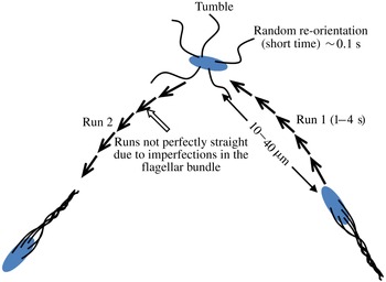
A bacterium typically runs in a directed sense for a certain time interval before changing its orientation abruptly, and by a large amount. It then runs in a new direction, possibly correlated to the old one. The change in orientation is termed a tumble, and is usually of a much smaller duration. For wild-type E. coli, the mean-run-time is
 ${\it\tau}\sim O(1~\text{s})$
, while the tumbles are almost instantaneous lasting only approximately 0.1 s (see figure 3). In a chemically homogeneous medium, the run-and-tumble statistics are well approximated by a Poisson process (Berg Reference Berg1993), the time between successive tumbles being exponentially distributed with a mean
 ${\it\tau}$
. A second parameter,
 ${\it\beta}$
, characterizes the correlation between the pre (
 $\boldsymbol{p}$
)- and post (
 $\boldsymbol{p}^{\prime }$
)-tumble orientations, being defined by
 $\langle \boldsymbol{p}\boldsymbol{\cdot }\boldsymbol{p}^{\prime }\rangle =(\coth {\it\beta}-1/{\it\beta})$
. The run-and-tumble motion, on large scales, is characterized by a translational diffusivity given by
 $({\it\beta}/(3[({\it\beta}+1)-{\it\beta}\coth {\it\beta}]))U^{2}{\it\tau}$
with
 ${\it\beta}=\infty$
and
 ${\it\beta}=0$
corresponding to perfectly correlated and random tumbles, respectively. Subramanian & Koch (Reference Subramanian and Koch2009) found that the threshold concentration for collective motion changed little for
 ${\it\beta}=1$
(the forward correlation observed in E. coli; Berg (Reference Berg1993)) relative to its value for random tumbles. Thus, in our simulations we assume that the tumbles are instantaneous and perfectly random with the long-time translational diffusivity, due to tumbles alone, being given by
 $U^{2}{\it\tau}/3$
.
A schematic of the run-and-tumble motion executed by peritrichously flagellated swimmers such as E. coli (Subramanian & Nott Reference Subramanian and Nott2012).

The implementation of the Poissonian statistics makes use of the fact that the probability per unit time that a given run ends is constant. Defining the mean tumble frequency as
 ${\it\lambda}=1/{\it\tau}$
, the probability of a tumble occurring in a given interval
 ${\rm\Delta}t$
is
 ${\it\lambda}{\rm\Delta}t$
. Although this expression is strictly valid only when
 ${\rm\Delta}t$
is a differential quantity, the time step used in our simulations is small enough for this relation to hold. To decide whether a swimmer tumbles during a given time step, a uniform random variable in the interval
 $(0,1)$
is generated. If this number is less than
 ${\it\lambda}{\rm\Delta}t$
, then a tumble is implemented by choosing a new swimmer orientation with a uniform probability on the unit sphere.
2.4.2. Rotary diffusion
While tumbling causes large impulsive changes in swimmer orientation, there are small-amplitude orientation fluctuations even during a run (see figure 3), attributed to imperfections in the flagellar bundle in the case of E. coli (Subramanian & Nott Reference Subramanian and Nott2012); E. coli tracks between successive tumbles show a mean deviation of around 27 degrees from a straight line (Berg Reference Berg1993). These small changes in orientation can be modelled as a rotary diffusion process. We simulate rotary diffusion via a two-dimensional random walk on the local tangent plane. The angular displacement in a time
 ${\rm\Delta}t$
is added as a random displacement of amplitude
 $A$
(Grassia, Hinch & Nitsche Reference Grassia, Hinch and Nitsche1995),
 ${\rm\Delta}{\it\theta}=AR_{n}$
, where
 $R_{n}$
is uniformly distributed in the interval
 $[-1/2,1/2]$
. As a result,
 $\langle ({\rm\Delta}{\it\theta})^{2}\rangle =A^{2}\langle R_{n}^{2}\rangle =A^{2}/12=4D_{r}{\rm\Delta}t$
, which gives
 $A=(48D_{r}{\rm\Delta}t)^{1/2}$
. This specifies a cone of half-angle
 ${\rm\Delta}{\it\theta}$
about the swimmer’s initial orientation, and the additional angle
 ${\it\phi}$
that specifies the location on this cone is uniformly distributed in
 $[0,2{\rm\pi}]$
.
Both the tumbling and rotary diffusion models described above have been validated by comparing the swimmer mean-square-displacement and orientation decorrelation functions
 $\langle \boldsymbol{p}(0)\boldsymbol{\cdot }\boldsymbol{p}(t)\rangle$
and
 $\langle [\boldsymbol{p}(0)\boldsymbol{\cdot }\boldsymbol{p}(t)]^{2}\rangle$
with known theoretical results (
 $\langle r^{2}(t)\rangle =2(U{\it\tau})^{2}[t/{\it\tau}-1+\exp (-t/{\it\tau})]$
,
 $\langle \boldsymbol{p}(0)\boldsymbol{\cdot }\boldsymbol{p}(t)\rangle =\exp (-t/{\it\tau})$
,
 $\langle [\boldsymbol{p}(0)\boldsymbol{\cdot }\boldsymbol{p}(t)]^{2}\rangle =(2\exp (-t/{\it\tau})+1)/3$
, for tumbling;
 $\langle r^{2}(t)\rangle =(U/2D_{r})^{2}[2D_{r}t-1+\exp (-2D_{r}t)]$
,
 $\langle \boldsymbol{p}(0)\boldsymbol{\cdot }\boldsymbol{p}(t)\rangle =\exp (-2D_{r}t)$
for rotary diffusion).
2.5. Simulation algorithm
The initial condition is specified by initializing the swimmer positions (
 $\boldsymbol{X}\equiv \{\boldsymbol{x}_{1},\boldsymbol{x}_{2}\ldots \boldsymbol{x}_{N}\}$
) and orientations (
 $\boldsymbol{P}\equiv \{\boldsymbol{p}_{1},\boldsymbol{p}_{2}\ldots \boldsymbol{p}_{N}\}$
) in the simulation box. The positions are uniformly distributed in the simulation box and the orientations are uniformly distributed on the unit sphere. Note that the swimmers are assumed to be infinitely slender, and excluded volume considerations do not come into play in the choice of the initial configuration. In light of the known results for passive rod suspensions (Larson Reference Larson1988), we neglect their role in the dynamics also, since the volume fractions examined here are within the dilute regime. With the positions and orientations known, we can compute the velocity disturbance at the quadrature points along the length of each swimmer using (2.8). Once the velocity disturbance is known along the length of all swimmers, we can use (2.13) and (2.14) to calculate the translational and angular velocities. Formally, one may write the evolution equations as:
 $$\begin{eqnarray}\displaystyle \dot{\boldsymbol{X}} & = & \displaystyle \mathscr{F}(\boldsymbol{X},\boldsymbol{P}),\end{eqnarray}$$
 $$\begin{eqnarray}\displaystyle \dot{\boldsymbol{P}} & = & \displaystyle \mathscr{G}(\boldsymbol{X},\boldsymbol{P}),\end{eqnarray}$$
 $\mathscr{F}$
and
 $\mathscr{G}$
are known functionals of the velocity disturbance field. The positions and orientations of all the swimmers are updated using a second-order Runge–Kutta scheme (Wheatley & Gerald Reference Wheatley and Gerald1984), with a time step small enough to ensure converged results. For tumblers, the swimmers which tumble during the current time step are updated with a new orientation according to the model in § 2.4.1. For rotary diffusers, a small noise is added to the orientation vector of all the swimmers according to the model in § 2.4.2. The updated positions and orientations are used in the next time step, and so on.
3. Collective motion in a suspension of straight swimmers; model validation
In this section we discuss the results for straight swimmers, the main motivation being to validate our simulation methodology; specifically, the assumption that the intrinsic stress alone is sufficient to capture the salient aspects of collective motion. Earlier efforts have focused on such straight swimmers modelled either as slender rods with the inclusion of both intrinsic and induced stresses (Saintillan & Shelley Reference Saintillan and Shelley2007, Reference Saintillan and Shelley2012), or as regularized point dipoles (Underhill et al. Reference Underhill, Hernandez-Ortiz and Graham2008; Hernandez-Ortiz, Underhill & Graham Reference Hernandez-Ortiz, Underhill and Graham2009). We will present results for both pushers and pullers, with pullers serving only as a contrast that helps identify the onset of collective motion. We use various statistical measures involving the swimmers, the suspending fluid and passive tracer particles to compare our results with earlier efforts. Since linear stability theory predicts a long wavelength instability for an unbounded suspension of straight swimmers (pushers) for any non-zero volume fraction, it is only the finite size simulation box that stabilizes a straight-swimmer suspension. It is therefore crucial to study the effects of varying box size, and compare the box-size-dependent threshold for straight-swimming pushers, obtained from our simulations, with (1.5) in § 1.
The
 $x_{1}x_{2}$
projections of fluid velocity vectors lying in the midplane (with respect to
 $x_{3}$
) of the simulation box, for (a,b)
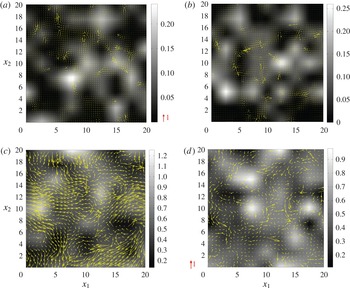
 ${\it\nu}=0.05$
(400 swimmers) and (c,d)
 ${\it\nu}=0.5$
(4000 swimmers), for both pushers and pullers (
 $L_{box}=10L$
). The grey-scale denotes the swimmer number density fields at the same instant. The red arrow denotes a vector of magnitude 1.

3.1. Fluid velocity statistics
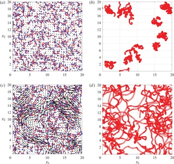
Figure 4(a–d) show typical fluid velocity fields and the associated number density fields in suspensions of pushers and pullers, with volume fractions of
 $0.05$
and
 $0.5$
, at a single time instant in the statistical steady state. At the lower volume fraction, the velocity fluctuations are only those due to individual uncorrelated swimmers which die off rapidly as one moves away from the particular swimmer (figure 4
a,b). In the suspension of pushers, as one moves to larger volume fractions, one begins to see coherent jets and vortices in the fluid on length scales larger than the swimmer size (see figure 4
c), similar to those observed in experiments (Mendelson et al.
Reference Mendelson, Bourque, Wilkening, Anderson and Watkins1999; Dombrowski et al.
Reference Dombrowski, Cisneros, Chatkaew, Goldstein and Kessler2004; Sokolov et al.
Reference Sokolov, Aranson, Kessler and Goldstein2007), and in agreement with previous simulations (Saintillan & Shelley Reference Saintillan and Shelley2007, Reference Saintillan and Shelley2012). Pullers, however, continue to show an uncorrelated velocity field at larger volume fractions dominated by small-scale fluctuations corresponding to individual swimmers (figure 4
d). Although not shown here, the number density fluctuations for pushers and pullers at both volume fractions adhere closely to Poissonian statistics with
 $\langle N^{2}\rangle ^{1/2}\sim \langle N\rangle ^{1/2}$
; we find no evidence of the giant number density fluctuations predicted/observed in other realizations of active matter (Simha & Ramaswamy Reference Simha and Ramaswamy2002; Narayan, Ramaswamy & Menon Reference Narayan, Ramaswamy and Menon2007) either in the stable or unstable regimes (for pushers).
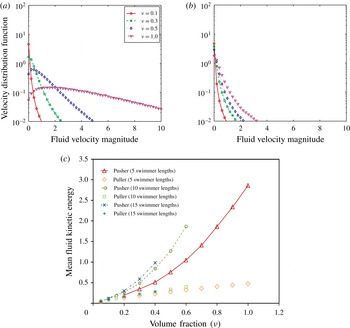
The above qualitative observations are confirmed on examination of the probability distributions of the individual fluid velocity components (not shown) as well as the magnitude. Both measures indicate much larger fluctuations for pushers at higher volume fractions. In particular, the probability density for the velocity magnitude (figure 5
a,b) displays clear evidence of bulk fluid motion since, beyond a critical volume fraction, the distribution peaks at a non-zero speed of order unity. In contrast, the peak for pullers seems to occur at a much smaller value not resolved in the plots shown. The enhancement for pushers can also be seen in the plot of the mean fluid kinetic energy versus volume fraction in figure 5(c). The pusher kinetic energy curve diverges from the puller curve with increasing volume fraction, with larger boxes leading to larger kinetic energies and a steeper rate of increase with
 ${\it\nu}$
. This is consistent with linear stability theory in that the larger box sizes allow a greater range of unstable wavelengths, and thus a more intense fluid motion. Pullers do not display a noticeable trend with box size.
Fluid velocity statistics. (a,b) Probability distribution function of fluid disturbance velocity magnitude (
 $L_{box}=10L$
). (c) Mean fluid kinetic energy plotted with respect to
 ${\it\nu}$
, for pushers and pullers, for three box sizes (
 $L_{box}=5L,10L$
and
 $15L$
). The volume fraction
 ${\it\nu}=1.0$
corresponds to 1000, 8000 and 27 000 swimmers for the box sizes of
 $5L$
,
 $10L$
and
 $15L$
, respectively.

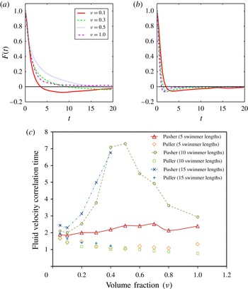
(a,b) The fluid velocity autocorrelation function,
 $F(t)$
, plotted for pushers and pullers at different volume fractions. (c) The correlation times for pushers and pullers plotted with respect to
 ${\it\nu}$
for
 $L_{box}=5L$
,
 $10L$
and
 $15L$
. The volume fraction
 ${\it\nu}=1.0$
corresponds to 1000, 8000 and 27 000 swimmers for the three box sizes
 $5L$
,
 $10L$
and
 $15L$
, respectively.

Further evidence of differences between pushers and pullers can be seen from plots of the Eulerian fluid velocity correlation, shown in figure 6(a,b), for pushers and pullers at different volume fractions. Figure 6(c) shows the correlation times, extracted from figure 6(a,b) by assuming an exponential decay, plotted as a function of the volume fraction (there is no rigorous basis for expecting an exponential decay since the correlation functions clearly change sign for intermediate times; the simple exponential fit nevertheless gives reasonable estimates). For pushers, the correlation time shows an initial increase with volume fraction reaching a maximum around
 ${\it\nu}=0.5$
. At these volume fractions, correlated fluid motions are persistent over time scales much larger than the single swimmer time scale of
 $L/2U$
(
 $7$
times larger at
 ${\it\nu}=0.5$
for the
 $10$
-swimmer-length box). Further increase in the volume fraction leads to a decrease in the correlation times due to the dominant effect of a given point in space randomly sampling swimmer velocity fields at an increased frequency. The trend for pullers is clearly different in that puller suspensions show a monotonic decrease in the correlation times with volume fraction as seen in figure 6(b). This decrease may be attributed to the same effect which caused the decrease in pusher correlation times for higher volume fractions, mentioned above. The effect of box size can again be seen in figure 6(c) with larger simulation boxes (
 $10$
and
 $15$
-swimmer-lengths) leading to much larger correlation times. Our focus, in trying to identify a stability threshold, will henceforth be restricted to
 ${\it\nu}\leqslant 0.6$
where the pusher correlation times increase with increasing volume fraction.
3.2. Swimmer statistics
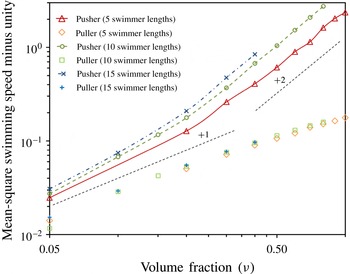
The swimmer speed in a suspension deviates from its isolated value (of unity) owing to hydrodynamic interactions. To quantify this, in figure 7, the enhancement in the mean-squared swimming speed versus volume fraction, for pushers and pullers, is shown for three different box sizes. Beyond a critical volume fraction, there is a clear pusher–puller bifurcation. The pushers transition from a linear to a quadratic scaling with increasing volume fraction, while the pullers exhibit a linear increase over the entire range of volume fractions considered. The linear increase is consistent with the enhancement arising due to convection by the fluid velocity field which in turn may be estimated from an independent-swimmer argument. This latter observation is consistent with the findings of Hernandez-Ortiz et al. (Reference Hernandez-Ortiz, Underhill and Graham2009) for regularized dipole swimmers in a confined domain. Further, unlike pullers, the effect of box size on pusher speeds is noticeable in figure 7. Note that the increase in puller speed with volume fraction found here is unlike the weak decrease reported by Saintillan & Shelley (Reference Saintillan and Shelley2012), a discrepancy that may arise from the neglect of induced stresses.
Mean-square swimming speed minus unity plotted with respect to
 ${\it\nu}$
, for pushers and pullers, for
 $L_{box}=5L$
,
 $10L$
and
 $15L$
.

Next, we look at the polar pair orientation correlation defined as (Saintillan & Shelley Reference Saintillan and Shelley2007):
 $$\begin{eqnarray}C_{1}(r)=\frac{\displaystyle \left\langle \mathop{\sum }_{i\neq j}\boldsymbol{p}_{i}\boldsymbol{\cdot }\boldsymbol{p}_{j}{\it\delta}(|\boldsymbol{x}_{i}-\boldsymbol{x}_{j}|-r)\right\rangle }{\displaystyle \left\langle \mathop{\sum }_{i\neq j}{\it\delta}(|\boldsymbol{x}_{i}-\boldsymbol{x}_{j}|-r)\right\rangle },\end{eqnarray}$$
for both pushers and pullers. The polar correlation function above distinguishes between parallel (
 $C_{1}=1$
) and anti-parallel (
 $C_{1}=-1$
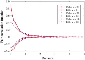
) swimmer alignments. We see from figure 8 that pushers and pullers show strong positive and negative correlations, respectively, at the volume fractions examined, and for separations of order the swimmer length. These aligning tendencies likely arise from pair interactions in the stable regime, and the decrease in the near-contact value of the correlation with increasing
 $nL^{3}$
suggests that higher volume fractions impede the effects of pair interactions for both pushers and pullers. Since our results compare well with Saintillan & Shelley (Reference Saintillan and Shelley2007) we conclude that the intrinsic stresses alone are sufficient to capture the main effects of the pair correlations, even in the stable regime. The general features of the orientation correlations, such as the opposing signs for pushers and pullers and the secondary role of the induced stresses, are consistent with what one might expect from viscous slender body theory at leading logarithmic order. A careful examination of figure 8 also reveals subtle signatures of the instability. Pushers show stronger correlations at a given separation, larger correlation lengths and importantly, the correlation length increases with increasing volume fraction, indicative of contributions arising from long-wavelength velocity fluctuations.
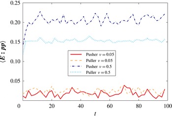
Another statistical measure of interest is the degree of alignment of a given swimmer along the local extensional axis of the ‘ambient’ rate-of-strain tensor resulting from the cumulative effect of the velocity disturbances due to all other swimmers. In the case of pushers, as discussed earlier, this alignment leads to an orientational anisotropy which reinforces the velocity disturbance, leading to an exponential instability (see Subramanian & Koch Reference Subramanian and Koch2009). In figure 9, we plot
 $\boldsymbol{E}\boldsymbol{ : }\boldsymbol{p}\boldsymbol{p}$
averaged over all the swimmers with respect to time. Both pushers and pullers show a weak parallel alignment at the lower volume fraction. At the higher volume fraction, the alignment is greater for pushers, consistent with the mutual reinforcement of velocity and orientation fluctuations that underlies the linear stability scenario (Subramanian & Koch Reference Subramanian and Koch2009; Subramanian & Nott Reference Subramanian and Nott2012).
The polar pair-correlation function as a function of distance from the test swimmer for
 ${\it\nu}=0.1$
,
 ${\it\nu}=0.5$
and
 ${\it\nu}=1.0$
;
 $L_{box}=10L$
(
 ${\it\nu}=1.0$
corresponds to 8000 swimmers).

 $\langle \boldsymbol{E}\boldsymbol{ : }\boldsymbol{p}\boldsymbol{p}\rangle$
, a measure of the swimmer alignment with the local extensional axis, as a function of time;
 $L_{box}=10L$
(
 ${\it\nu}=0.5$
corresponds to 4000 swimmers).

3.3. Tracer transport
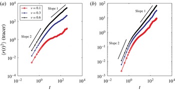
In this section we study the transport of passive non-Brownian tracer particles convected by the swimmer disturbance fields, motivated by one of the earliest experiments on bacterial suspensions by Wu & Libchaber (Reference Wu and Libchaber2000) which involved the measurement of tracer diffusivities to characterize the presence of large-scale correlated motion in a freely standing soap film with swimming bacteria. Figure 10 shows the time evolution of tracer mean-square displacements. An initial ballistic regime is followed by long-time diffusive behaviour. The mean-square displacements in pusher and puller suspensions are comparable at low volume fractions (
 ${\it\nu}=0.1$
). However, there is a remarkable increase for pushers at higher volume fractions with the displacements exceeding those of pullers by around two orders of magnitude at
 ${\it\nu}=0.6$
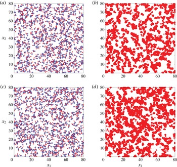
. This is consistent with dramatic differences between the tracer trajectories in pusher and puller suspensions (figure 11). For pullers, the tracer particles execute a random walk with no significant persistence (figure 11
a,b). In striking contrast, the tracer trajectories in pusher suspensions show significant correlated motions, filling up the entire field of view (figure 11
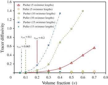
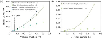
c,d). The tracer diffusivities are plotted as a function of the swimmer volume fraction in figure 12, wherein the pusher curves show a clear bifurcation beyond a critical volume fraction with diffusivities that are much larger than those for pullers. Importantly, the simulation box size has a marked effect, with the bifurcation point shifting to lower volume fractions as the box size is increased. This is due to tracer diffusivities for pushers, at a given volume fraction (beyond the bifurcation point), increasing with increasing box size. The bifurcation point is in good agreement with that predicted by the linear theory (see (1.5)). The puller curves seem fairly box-size-independent, pointing to the absence of any instability and collective motion. While this is the case for the straight swimmers examined here, a non-trivial box-size-dependence will be seen to arise later in the presence of an intrinsic decorrelation mechanism (see §§ 4.2.2 and 4.3).
Among all statistical measures considered here, the tracer diffusivity is the most sensitive measure of the onset of collective motion. This can be seen by comparing figure 12 with earlier plots of the mean fluid kinetic energy (figure 5
c) and fluid velocity correlation times (figure 6
c), and is consistent with earlier simulations by Saintillan & Shelley (Reference Saintillan and Shelley2012); the diffusivity values and fluid velocity fluctuations in our simulations are consistently greater than those in Saintillan & Shelley (Reference Saintillan and Shelley2012) owing to our neglect of induced stresses. The tracer diffusivity scales as
 $D_{tracer}\sim \langle u^{2}\rangle {\it\tau}_{corr}$
. Both the fluid velocity magnitude (
 $\langle u^{2}\rangle ^{1/2}$
) and correlation time (
 ${\it\tau}_{corr}$
) show an increasing trend with volume fraction after the onset of collective motion, and the combined effect is to cause an even larger increase in the trace diffusivity for pushers. Underhill et al. (Reference Underhill, Hernandez-Ortiz and Graham2008) find similar results in their simulations with the tracer diffusivity in pusher suspensions exhibiting a pronounced box-size-dependence; in their case, however, the box-size-dependence is primarily due to a similar dependence of the correlation time. In what follows, we will use the tracer diffusivity to identify the box-size-independent threshold for instability in a suspension of pushers that undergo a run-and-tumble motion. As will be seen, the pusher–puller bifurcation in this case is much more subtle, and the choice of a sensitive statistical measure is indeed crucial.
To summarize, based on the fluid, swimmer and tracer statistics for straight-swimmer suspensions, our kinematic simulations appear to faithfully capture most of the salient features of the collective motion for pusher suspensions, as reported in earlier simulation efforts (Saintillan & Shelley Reference Saintillan and Shelley2007, Reference Saintillan and Shelley2012; Underhill et al. Reference Underhill, Hernandez-Ortiz and Graham2008), and this remains true for both the stable and unstable regimes.
Mean-square displacements for the tracer particles plotted with respect to time for (a) pushers and (b) pullers;
 $L_{box}=10L$
.

Simulation snapshots showing the (straight) swimmer positions (blue circles), orientations (red arrows) and the fluid disturbance velocity vectors (black arrows) on (a,c) at
 $t=100$
and tracer trajectories, integrated over the period
 $t=0{-}100$
, on (b,d). (a,b) Puller suspension and (c,d) pusher suspension;
 $L_{box}=10L$
with
 ${\it\nu}=0.5$
(4000 swimmers). The figures only display swimmers and tracers in a slab of size
 $20\times 20\times 3$
in the
 $x_{1}$
,
 $x_{2}$
and
 $x_{3}$
directions, respectively, centred around the midplane of the simulation box (along
 $x_{3}$
). The fluid velocity vectors are projected onto this midplane.

Tracer diffusivities as a function of
 ${\it\nu}$
, for pushers and pullers, for
 $L_{box}=5L$
,
 $10L$
and
 $15L$
. The vertical lines indicate the box-size-dependent theoretical predictions given by (1.5).

4. Collective motion in a suspension of tumblers and rotary diffusers
In this section our main focus will be the impact of intrinsic orientation relaxation mechanisms on the onset of collective motion in pusher suspensions. We seek to identify the stability thresholds for suspensions of both tumblers and rotary diffusers based on our simulations, and to compare the same with the box-size-independent thresholds predicted by Subramanian & Koch (Reference Subramanian and Koch2009). As already noted, this box-size-independence is in sharp contrast to the case of straight swimmers.
4.1. Theory for tracer diffusion in a suspension of tumblers
Prior to discussing the simulation results, we discuss existing theoretical work related to tracer transport in a dilute stable swimmer suspension. Lin, Thiffeault & Childress (Reference Lin, Thiffeault and Childress2011) considered tracer transport in a suspension of spherical squirmers that execute a run-and-tumble motion with constant run lengths (
 $U{\it\tau}$
constant) using a kinetic theory approach first employed by Thiffeault & Childress (Reference Thiffeault and Childress2010). In the limit
 $U{\it\tau}\gg L$
, the dominant contribution to the tracer diffusivity was found to come from the
 $O(1/r^{2})$
stresslet velocity field, and scaled as
 $nUL^{4}$
,
 $n$
being the swimmer number density, and was therefore independent of
 ${\it\tau}$
. Interestingly, Pushkin & Yeomans (Reference Pushkin and Yeomans2013) showed that the tracer diffusivity in a suspension of swimming (point) force dipoles, that undergo a similar run-and-tumble motion, is, in fact, independent of
 ${\it\tau}$
for any
 $U{\it\tau}/L$
, on account of the self-similar nature of the
 $O(1/r^{2})$
velocity field associated with a point dipole, a conclusion also reached by Kasyap, Koch & Wu (Reference Kasyap, Koch and Wu2014). Miño et al. (Reference Miño, Dunstan, Rousselet, Clément and Soto2013) considered tracer diffusion arising in a suspension of straight swimmers, and surprisingly, the leading-order scaling for the diffusivity differed from the large-
 ${\it\tau}$
scaling of Lin et al. (Reference Lin, Thiffeault and Childress2011). The difference arises from the vanishing of the tracer displacement in the Eulerian approximation (fixed tracer location), due to the symmetry of the swimmer-induced displacements; indeed, even the classical calculation of the drift induced by a translating passive particle (Darwin Reference Darwin1953), with a fore–aft symmetric potential flow field, crucially relies on the Lagrangian asymmetry resulting from the convection of the tracer particle. As shown by Kasyap et al. (Reference Kasyap, Koch and Wu2014), and explained below, the discrepancy between Lin et al. (Reference Lin, Thiffeault and Childress2011) and Miño et al. (Reference Miño, Dunstan, Rousselet, Clément and Soto2013) points to the deterministic swimmer not being the same as a tumbler in the limit of a vanishingly small tumble frequency. In other words, the limit of vanishingly small stochasticity is a singular one as far as the tracer diffusivity scaling is concerned. More recently, Morozov & Marenduzzo (Reference Morozov and Marenduzzo2014), have again considered dipolar swimmers characterized by a constant path length, and find a tracer diffusivity
 $D=AnU{\it\sigma}^{4}$
similar to Lin et al. (Reference Lin, Thiffeault and Childress2011). Based on numerical simulations, the authors show that the prefactor
 $A$
goes to zero for large
 $U{\it\tau}/L$
. It was shown by Pushkin & Yeomans (Reference Pushkin and Yeomans2014) that this is due to the finite system size in the simulations, but a clear explanation for this non-trivial effect was not given, and neither was an expression for the tracer diffusivity in a periodic-box derived by rigorously accounting for hydrodynamic interactions with image swimmers.
The tracer diffusivity calculation most relevant to a suspension of slender-bodied swimmers that undergo a run-and-tumble dynamics, with the run-lengths governed by a Poisson distribution, is that of Kasyap et al. (Reference Kasyap, Koch and Wu2014). The diluteness assumption allowed the authors to neglect swimmer–swimmer and swimmer–tracer correlations, and each tracer particle is, at any given time, convected by the velocity field due to a single swimmer. As pointed out earlier in the context of the simulations by Graham and co-workers, a slender swimmer model, apart from being a more faithful representation of bacteria such as E. coli or B. subtilis, has the additional important advantage of avoiding a regularization length scale. Kasyap et al. (Reference Kasyap, Koch and Wu2014) found the tracer diffusivity to be of the form
 $D_{h}=nUL^{4}\widetilde{D}_{h}$
, where
 $\widetilde{D}_{h}$
is a monotonically increasing function of the non-dimensional mean-run-time
 $U{\it\tau}/L$
with
 $\widetilde{D}_{h}\rightarrow 1/(768{\rm\pi}M^{2})$
for
 $U{\it\tau}/L\rightarrow \infty$
(
 $M$
here being the mobility of the swimmer head). For nearly straight swimmers (
 $U{\it\tau}/L\gg 1$
), the contribution to the tracer diffusivity comes from length scales much larger than the swimmer length, or equivalently, from asymptotically small wavenumbers in the tracer diffusion integral (see (4.1) below) where tumbling remains important. This peculiarity implies, as mentioned above, that the limit of a vanishing rate of relaxation (either tumbling or rotary diffusion) is a singular one. This also raises an interesting question regarding the tracer diffusivity in a periodic-box, relevant to our simulations, where the finite contribution due to distant tumbles will not occur once the swimmer trajectory exceeds the box dimensions.
Starting from equation (21) in Kasyap et al. (Reference Kasyap, Koch and Wu2014) for the tracer diffusivity in an unbounded swimmer suspension, given by the following integral of the Fourier transformed swimmer velocity field:
 $$\begin{eqnarray}D_{h}=\frac{n}{12{\rm\pi}}\int \text{d}\boldsymbol{p}\int \text{d}\boldsymbol{k}\frac{\hat{\boldsymbol{U}}(\boldsymbol{k})\boldsymbol{\cdot }\hat{\boldsymbol{U}}(-\boldsymbol{k})}{\displaystyle (2{\rm\pi}k)^{2}D+2{\rm\pi}\text{i}\boldsymbol{k}\boldsymbol{\cdot }\boldsymbol{p}U+\frac{1}{{\it\tau}}},\end{eqnarray}$$
the tracer diffusivity in a spatially periodic setting is given by:
 $$\begin{eqnarray}D_{h}=\frac{n}{12{\rm\pi}L_{box}^{3}}\int \text{d}\boldsymbol{p}\mathop{\sum }_{\boldsymbol{k}\neq 0}\frac{\hat{\boldsymbol{U}}(\boldsymbol{k})\boldsymbol{\cdot }\hat{\boldsymbol{U}}(-\boldsymbol{k})}{\displaystyle (2{\rm\pi}k)^{2}D+2{\rm\pi}\text{i}\boldsymbol{k}\boldsymbol{\cdot }\boldsymbol{p}U+\frac{1}{{\it\tau}}},\end{eqnarray}$$
where the integral over wavenumber space is simply replaced by a summation over discrete wavevectors normalized by the volume of the simulation box. Here,
 $\hat{\boldsymbol{U}}(\boldsymbol{k})=\int \text{d}\boldsymbol{x}\,\boldsymbol{u}^{\prime }(\boldsymbol{x})\text{e}^{-2{\rm\pi}\text{i}\boldsymbol{k}\boldsymbol{\cdot }\boldsymbol{x}}$
,
 $\boldsymbol{u}^{\prime }(\boldsymbol{x})$
being the spatially periodic velocity field due to an infinite cubic array of swimmers. The tracer above is considered to be Brownian with a diffusivity
 $D$
. The expression for
 $\hat{\boldsymbol{U}}(\boldsymbol{k})$
is given by:
 $$\begin{eqnarray}\hat{\boldsymbol{U}}(\boldsymbol{k})=\frac{UL_{box}^{3}}{Mk^{2}}\left[\boldsymbol{p}-\frac{(\boldsymbol{k}\boldsymbol{\cdot }\boldsymbol{p})\boldsymbol{k}}{k^{2}}\right]F(\boldsymbol{k}\boldsymbol{\cdot }\boldsymbol{p}),\end{eqnarray}$$
where
 $F(\boldsymbol{k}\boldsymbol{\cdot }\boldsymbol{p})$
is related to the swimmer (line) force distribution, and is given by Kasyap et al. (Reference Kasyap, Koch and Wu2014):
 $$\begin{eqnarray}F(\boldsymbol{k}\boldsymbol{\cdot }\boldsymbol{p})=-\frac{1}{\text{i}\boldsymbol{k}\boldsymbol{\cdot }\boldsymbol{p}}\left\{\text{e}^{-((\text{i}{\it\alpha}_{1}\boldsymbol{k}\boldsymbol{\cdot }\boldsymbol{p})/2)L/L_{box}}-\frac{1}{1-{\it\alpha}_{1}}\text{e}^{((\text{i}{\it\alpha}_{1}\boldsymbol{k}\boldsymbol{\cdot }\boldsymbol{p})/2)L/L_{box}}+\frac{{\it\alpha}_{1}}{1-{\it\alpha}_{1}}\text{e}^{\text{i}[1-{\it\alpha}_{1}/2]\boldsymbol{k}\boldsymbol{\cdot }\boldsymbol{p}L/L_{box}}\right\}.\vphantom{\mathop{\sum }_{a}}\end{eqnarray}$$
In (4.3) and (4.4), the wavevector is scaled by the factor
 $(2{\rm\pi}L_{box})^{-1}$
. Substituting (4.3) and (4.4) in (4.2), and rescaling the terms in the denominator, we obtain:
 $$\begin{eqnarray}\displaystyle D_{h}=nL^{3}UL\left(\frac{L_{box}}{L}\right)^{3}\frac{1}{12{\rm\pi}M^{2}}\int \text{d}\boldsymbol{p}\mathop{\sum }_{\boldsymbol{k}\neq 0}\frac{[k^{2}-(\boldsymbol{k}\boldsymbol{\cdot }\boldsymbol{p})^{2}]F(\boldsymbol{k}\boldsymbol{\cdot }\boldsymbol{p})F(-\boldsymbol{k}\boldsymbol{\cdot }\boldsymbol{p})}{k^{6}\left[\displaystyle \frac{k^{2}}{Pe}\frac{L^{2}}{L_{box}^{2}}+\text{i}\boldsymbol{k}\boldsymbol{\cdot }\boldsymbol{p}\frac{L}{L_{box}}+\frac{2}{{\it\tau}}\right]}, & & \displaystyle\end{eqnarray}$$
where we have rescaled
 ${\it\tau}$
by
 $L/(2U)$
, and
 $Pe=UL/D$
. For our simulations,
 ${\it\alpha}_{1}=1/2$
, and one obtains:
 $$\begin{eqnarray}F(\boldsymbol{k}\boldsymbol{\cdot }\boldsymbol{p})F(-\boldsymbol{k}\boldsymbol{\cdot }\boldsymbol{p})=\frac{16\sin ^{4}\left(\displaystyle \frac{\boldsymbol{k}\boldsymbol{\cdot }\boldsymbol{p}}{4}\frac{L}{L_{box}}\right)}{(\boldsymbol{k}\boldsymbol{\cdot }\boldsymbol{p})^{2}}.\end{eqnarray}$$
Substituting the above expression in (4.5), and considering
 $Pe\rightarrow \infty$
(a non-Brownian tracer, as is the case in the simulations), we find:
 $$\begin{eqnarray}\widetilde{D}_{h}=\frac{4}{3{\rm\pi}M^{2}}\left(\frac{1}{L^{\ast }}\right)^{3}\int \text{d}\boldsymbol{p}\mathop{\sum }_{\boldsymbol{k}\neq 0}\frac{\displaystyle [k^{2}-(\boldsymbol{k}\boldsymbol{\cdot }\boldsymbol{p})^{2}]\sin ^{4}\left(\frac{L^{\ast }\boldsymbol{k}\boldsymbol{\cdot }\boldsymbol{p}}{4}\right)}{\displaystyle (\boldsymbol{k}\boldsymbol{\cdot }\boldsymbol{p})^{2}k^{6}\left[\text{i}\boldsymbol{k}\boldsymbol{\cdot }\boldsymbol{p}L^{\ast }+\frac{2}{{\it\tau}}\right]},\end{eqnarray}$$
where we have denoted the ratio
 $L/L_{box}=L^{\ast }$
. Interchanging the integral and summation, and using a polar coordinate system aligned with
 $\hat{\boldsymbol{k}}$
, we have
 $\boldsymbol{k}\boldsymbol{\cdot }\boldsymbol{p}=k\cos {\it\theta}$
and
 $\text{d}\boldsymbol{p}=\sin {\it\theta}\,\text{d}{\it\theta}\,\text{d}{\it\phi}$
, and (4.7) can be written as:
 $$\begin{eqnarray}\widetilde{D}_{h}=\frac{8}{3M^{2}}\left(\frac{1}{L^{\ast }}\right)^{3}\mathop{\sum }_{\boldsymbol{k}\neq 0}\frac{1}{k^{6}}\int _{-1}^{1}\,\text{d}m\left(\frac{1-m^{2}}{m^{2}}\right)\frac{\displaystyle \sin ^{4}\left(\frac{kL^{\ast }m}{4}\right)}{\displaystyle \left[\text{i}kmL^{\ast }+\frac{2}{{\it\tau}}\right]},\end{eqnarray}$$
with
 $m=\cos {\it\theta}$
, which is the final expression for the non-dimensional tracer diffusivity in a spatially periodic (dilute) swimmer suspension.
For arbitrary
 ${\it\tau}$
, the integral and the
 $\boldsymbol{k}$
-summation in (4.8) are performed numerically. The analytical forms for
 ${\it\tau}\rightarrow 0$
and
 ${\it\tau}\rightarrow \infty$
follow immediately from (4.8). Considering first the
 ${\it\tau}\rightarrow 0$
limit, and expanding the denominator
 $(\text{i}kmL^{\ast }{\it\tau}/2+1)$
for small
 ${\it\tau}$
, gives:
 $$\begin{eqnarray}\widetilde{D}_{h}=\frac{8}{3M^{2}}\left(\frac{1}{L^{\ast }}\right)^{3}{\it\tau}\mathop{\sum }_{\boldsymbol{k}\neq 0}\frac{1}{k^{6}}\int _{0}^{1}\,\text{d}m\left(\frac{1-m^{2}}{m^{2}}\right)\sin ^{4}\left(\frac{kL^{\ast }m}{4}\right),\end{eqnarray}$$
where we have used the fact that the integrand is an even function of
 $m$
. From (4.9), the dimensional tracer diffusivity for small
 ${\it\tau}$
scales as
 $O(nL^{3})U^{2}{\it\tau}$
. An analogous small-
 ${\it\tau}$
asymptote may be obtained for an unbounded domain from (4.1), and corresponds to
 $D_{h}=1/(576{\rm\pi}M^{2})(nL^{3})U^{2}{\it\tau}$
. In either case, the tracer is convected, with a probability of
 $O(nL^{3})$
by a bacterium velocity field of
 $O(U)$
that decorrelates after a (short) time of
 $O({\it\tau})$
. With decreasing
 $L^{\ast }$
, the periodic-box asymptote approaches the unbounded estimate, implying that periodicity is a regular effect for
 ${\it\tau}\rightarrow 0$
.
For
 ${\it\tau}\rightarrow \infty$
, we rewrite (4.8) as:
 $$\begin{eqnarray}\widetilde{D}_{h}=\frac{8}{3M^{2}}\left(\frac{1}{L^{\ast }}\right)^{3}\mathop{\sum }_{\boldsymbol{k}\neq 0}\frac{1}{k^{6}}\int _{-1}^{1}\,\text{d}m\left(\frac{1-m^{2}}{m^{2}}\right)\frac{\displaystyle \sin ^{4}\left(\frac{kL^{\ast }m}{4}\right)}{\displaystyle \text{i}kmL^{\ast }\left[1+\frac{2}{\text{i}kmL^{\ast }{\it\tau}}\right]}.\end{eqnarray}$$
Expanding the denominator
 $[1+2/(\text{i}kmL^{\ast }{\it\tau})]$
for large
 ${\it\tau}$
, we obtain:
 $$\begin{eqnarray}\widetilde{D}_{h}=\frac{8}{3M^{2}}\left(\frac{1}{L^{\ast }}\right)^{3}\mathop{\sum }_{\boldsymbol{k}\neq 0}\frac{1}{k^{6}}\int _{-1}^{1}\,\text{d}m\left(\frac{1-m^{2}}{m^{2}}\right)\frac{\displaystyle \sin ^{4}\left(\frac{kL^{\ast }m}{4}\right)}{\displaystyle \text{i}kmL^{\ast }}\left[1-\frac{2}{\text{i}kmL^{\ast }{\it\tau}}\right].\end{eqnarray}$$
The integral in the first term is odd in
 $m$
and hence is zero. The second term, therefore, gives the leading-order contribution to the diffusivity as:
 $$\begin{eqnarray}\widetilde{D}_{h}=\frac{32}{3M^{2}}\left(\frac{1}{L^{\ast }}\right)^{5}\frac{1}{{\it\tau}}\mathop{\sum }_{\boldsymbol{k}\neq 0}\frac{1}{k^{8}}\int _{0}^{1}\,\text{d}m\left(\frac{1-m^{2}}{m^{4}}\right)\sin ^{4}\left(\frac{kL^{\ast }m}{4}\right).\end{eqnarray}$$
This leads to the counter-intuitive conclusion that the periodic-box tracer diffusivity vanishes in the limit
 ${\it\tau}\rightarrow \infty$
(nearly straight swimmers). This prediction (4.12) is in contrast to an unbounded suspension where a finite diffusivity emerges in this limit (Lin et al.
Reference Lin, Thiffeault and Childress2011; Kasyap et al.
Reference Kasyap, Koch and Wu2014). The mathematical reason for this can be deduced from (4.1) (see Kasyap et al.
Reference Kasyap, Koch and Wu2014) where, in the limit of large
 ${\it\tau}$
, the integral requires a Cauchy principal-value interpretation, the dominant contribution coming from wavenumbers of
 $O(1/U{\it\tau})$
or smaller. Physically, this corresponds to a sufficiently large number of distant tumbles continuing to break the symmetry of the (deterministic) swimmer–tracer interaction at leading order. However, in a periodic-box, we see from the denominator of (4.8) that the smallest wavenumber is
 $O(L^{\ast })$
. For
 $1/{\it\tau}\ll L^{\ast }$
(
 $(U{\it\tau})^{-1}\ll L_{box}^{-1}$
in dimensional terms), the dominant contribution in the unbounded case is not captured by the discrete sum over
 $\boldsymbol{k}$
. Thus, rather interestingly, the artefact of periodicity, inherent in any numerical simulation, renders the limit of vanishingly small stochasticity a regular one, in the sense of the large-
 ${\it\tau}$
limit being consistent with the zero tracer diffusivity obtained in the Eulerian fixed tracer approximation applied to a suspension of straight swimmers (Miño et al.
Reference Miño, Dunstan, Rousselet, Clément and Soto2013; Pushkin, Shum & Yeomans Reference Pushkin, Shum and Yeomans2013). It may be shown that the leading-order tracer diffusivity vanishes even for
 ${\it\alpha}_{1}\neq 1/2$
, and the above comments therefore remain valid for swimmers with asymmetric force distributions (as must be the case, since all such swimmers appear as point force dipoles in the far-field). The dimensionless (non-Brownian) tracer diffusivity is plotted in figure 13 for a number of box sizes along with the result for an unbounded suspension. The latter increases monotonically with
 ${\it\tau}$
with an
 $O(nUL^{4})$
large-
 ${\it\tau}$
asymptote. The periodic-box diffusivity, however, is non-monotonic with a maximum of
 $O(nUL^{4})$
at a finite
 ${\it\tau}$
of
 $O(L/U)$
; note that this maximum should spread out into a broad plateau in the range
 $L/U\ll {\it\tau}\ll L_{box}/U$
with increasing
 $L_{box}$
. The small and large
 ${\it\tau}$
asymptotes given by (4.9) and (4.12) are also shown.
Theoretical predictions for the tracer diffusivity in an unbounded suspension and in a periodic array of swimmers (
 $L_{box}=10L,15L$
and
 $25L$
). In the former case, the diffusivity monotonically increases to a
 ${\it\tau}$
-independent limit (solid black curve). The periodic-box results show a non-monotonic trend, with the small
 ${\it\tau}$
and large
 ${\it\tau}$
asymptotes being
 $O({\it\tau})$
and
 $O(1/{\it\tau})$
, respectively.

The non-trivial role of periodicity above is evidently relevant to our simulations. The
 $O(1/{\it\tau})$
scaling of the periodic-box tracer diffusivity, leading to the aforementioned non-monotonicity, results from two approximations in the above analysis – the approximation of a fixed tracer location and the neglect of hydrodynamic interactions between swimmers. As already pointed out, accounting for the tracer displacement during a swimmer–tracer interaction will lead to a non-zero tracer diffusivity as
 ${\it\tau}\rightarrow \infty$
, even in a spatially periodic setting, and such displacements occur naturally in the simulations discussed below; this effect is, however, small in the limit of slender swimmers owing to the weak disturbance field that convects the tracer. More importantly, in the presence of inter-swimmer hydrodynamic interactions, the decrease in the periodic-box tracer diffusivity, for large
 ${\it\tau}$
, will be cutoff once the rate of swimmer orientation decorrelation due to tumbles becomes comparable to that arising from hydrodynamic interactions. In other words, for large enough
 ${\it\tau}$
, the tracer diffusivity must approach a plateau controlled by the hydrodynamically induced orientation decorrelation arising from (weak) swimmer interactions. In the dilute regime, and for large aspect ratios (
 ${\it\gamma}\gg 1$
), this decorrelation arises from the cumulative effects of small
 $O(\ln {\it\gamma})^{-1}$
orientation changes associated with successive pair interactions, and may be characterized by a rotary diffusivity (Rahnama, Koch & Shaqfeh Reference Rahnama, Koch and Shaqfeh1995). This hydrodynamic rotary diffusivity
 $(D_{rh})$
for slender-bodied swimmers was calculated by Subramanian & Koch (Reference Subramanian and Koch2009), who found it to be
 $O[nUL^{2}/(\ln {\it\gamma})^{2}]$
for an unbounded domain. Now, from (4.12), the large-
 ${\it\tau}$
asymptote of the periodic-box tracer diffusivity is
 $O(nUL^{4}{\it\tau}^{-1})$
, or in dimensional terms
 $O(nL^{5}/{\it\tau})$
, and this decrease with
 ${\it\tau}$
will continue until
 ${\it\tau}\sim O(D_{rh}^{-1})$
when the tracer diffusivity curve should turn around, eventually saturating at a value of
 $O(nL^{5}D_{rh})\sim ((nL^{3})/(\ln {\it\gamma})^{2})O(nUL^{4})$
for
 ${\it\tau}D_{rh}\gg 1$
(on use of the above infinite-domain estimate for
 $D_{rh}$
valid for
 $L_{box}>O(UD_{rh}^{-1})$
). Thus, the non-monotonic box-size-dependence predicted above arises essentially due to the hydrodynamic orientation decorrelation being much weaker than the intrinsic decorrelation (due to tumbling or rotary diffusion) for the slender swimmers considered here, corresponding to
 $nL^{3}\ll O(\ln {\it\gamma})^{2}$
for large enough box sizes. In the other extreme, where the hydrodynamic interactions are strong and induce a decorrelation on a time scale much shorter than the
 $O(L_{box}/U)$
scale corresponding to periodicity, the rate of orientation decorrelation is given by
 $[1/{\it\tau}+2D_{rh}]^{-1}$
, and an estimate of the tracer diffusivity is obtained as
 $(nL^{3})U^{2}[1/{\it\tau}+2D_{rh}]^{-1}$
with
 ${\it\tau},D_{rh}^{-1}\ll L_{box}/U$
. This expression implies a monotonic increase of the tracer diffusivity with
 ${\it\tau}$
with a large-
 ${\it\tau}$
plateau of
 $O(nL^{3}U^{2}/D_{rh})$
. The decorrelation due to strong hydrodynamic interactions is not a diffusive process in orientation space, and
 $D_{rh}^{-1}$
here must merely be regarded as the inverse of a hydrodynamic decorrelation time (
 ${\it\tau}_{hyd}$
). Thus, for strong hydrodynamic interactions, the periodic-box tracer diffusivity must rise monotonically to its large-
 ${\it\tau}$
asymptote. It is clear then that the behaviour of the tracer diffusivity, as a function of
 ${\it\tau}$
, in a spatially periodic swimmer suspension, depends on the strength of the inter-swimmer hydrodynamic interactions; the interactions may be termed weak or strong depending on the magnitude of the hydrodynamic orientation decorrelation time in relation to the time scale associated with periodicity. The strength of the inter-swimmer hydrodynamic interactions is a sensitive function of the swimmer model with earlier simulations having considered both weakly (Saintillan & Shelley Reference Saintillan and Shelley2007, Reference Saintillan and Shelley2012) and strongly (Underhill et al.
Reference Underhill, Hernandez-Ortiz and Graham2008) interacting swimmers. Towards the end of this section, we show, in our simulations, that there is indeed a transition of the tracer diffusivity curves from a non-monotonic to a monotonic variation with
 ${\it\tau}$
with decreasing hydrodynamic decorrelation time.
Tracer diffusivities for both straight swimmers and tumblers with
 ${\it\tau}=1$
and
 ${\it\tau}=3$
, plotted as a function of volume fraction;
 $L_{box}=10L$
.

For slender swimmers, the above discussion shows that there exists an upper limit of
 ${\it\tau}\sim O(L_{box}/U)$
above which box size effects lead to a non-monotonic dependence of
 $D_{h}$
on
 $U{\it\tau}/L$
. However, the threshold criterion discussed earlier implies that
 ${\it\tau}$
must be greater than
 $O(nUL^{2})^{-1}$
for instability in a suspension of run-and-tumble swimmers. Thus, for the
 ${\it\tau}$
-varying simulations, considered in §§ 4.2.2 and 4.2.3, one only has a finite
 ${\it\tau}$
-window, given by
 $(nUL^{2})^{-1}<{\it\tau}<L_{box}/U$
, available for examining the transition to instability representative of an unbounded suspension. In particular, if the volume fraction chosen is too small (with the intent of rendering swimmer–swimmer correlations vanishingly small in the stable dilute regime), the lower bound would begin to approach
 $O(L_{box}/U)$
, and effects related to periodicity would become dominant.
4.2. Simulations of suspensions of tumblers
Since the parameter
 $nUL^{2}{\it\tau}$
is predicted to govern the transition to collective motion in a suspension of run-and-tumble swimmers (Subramanian & Koch Reference Subramanian and Koch2009), one may cross-over to the unstable regime by increasing
 $nL^{3}$
at a fixed
 ${\it\tau}$
or vice versa. We discuss the volume-fraction-varying and
 ${\it\tau}$
-varying simulations in sequence.
4.2.1. Effect of varying volume fraction at fixed
 ${\it\tau}\,({\it\tau}=1\text{ and }{\it\tau}=3)$

In this section, we present results for suspensions of pushers and pullers which tumble at a fixed rate, for two different box sizes (
 $L_{box}=10L$
and
 $15L$
), with varying volume fraction. For the most part, the results below correspond to
 ${\it\tau}=1$
, this particular choice allowing us to identify a sensible threshold for instability. The tracer diffusivities alone are plotted for
 ${\it\tau}=1$
and
 ${\it\tau}=3$
(figures 14 and 17). The latter value is chosen since it falls in the typical range encountered for wild-type E. coli (Berg & Brown Reference Berg and Brown1972, see figure 3) and B. subtilis (Ordal & Goldman Reference Ordal and Goldman1976), although we find pusher suspensions to be unstable in this case even for the smallest volume fraction simulated, preventing a threshold identification. In what follows, statistical measures related to the suspending fluid and swimmers are discussed, before focusing on the tracer diffusivity since, as shown before, this is the most sensitive measure of the onset of collective motion.
The first effect of tumbling is an overall stabilization relative to suspensions of straight swimmers. There is a large decrease in the tracer diffusivities for suspensions of pushers as
 ${\it\tau}$
decreases from
 $\infty$
to
 $1$
, while puller diffusivities remain virtually unaffected (see figure 14). Small but systematic differences between pushers and pullers continue to exist beyond a critical volume fraction, even for a finite
 ${\it\tau}$
, and these are of relevance in identifying a threshold. This can be seen in figure 15(a,b), which show the mean fluid kinetic energy and the (Eulerian) velocity autocorrelation function, respectively. In figure 15(a), the difference between the pusher and puller kinetic energies grows with increasing volume fraction with pushers having kinetic energies greater by around 45 % at
 ${\it\nu}=0.5$
. Unlike straight swimmers, these differences do not show a strong trend with box size. In figure 15(b), the correlation times for pullers shows a decrease with an increase in volume fraction for reasons already discussed. For pushers, in contrast, one sees a small increase in the correlation time related to instability onset. These trends are similar to those for straight swimmers (see figure 6). Small yet systematic differences are also seen from the plot of the mean swimming speed versus the volume fraction in figure 16, where the pushers show higher swimming speeds, the pusher–puller difference again growing with volume fraction.
Fluid velocity statistics for tumblers. (a) Mean fluid kinetic energy plotted with respect to
 ${\it\nu}$
(
 ${\it\tau}=1$
) for pushers and pullers;
 $L_{box}=10L$
and
 $15L$
. (b) Eulerian fluid velocity autocorrelation function for
 ${\it\tau}=1$
, and for
 ${\it\nu}=0.05$
and
 $0.5$
;
 $L_{box}=10L$
.

Mean-square swimming speed minus unity plotted with respect to volume fraction for pushers and pullers;
 $L_{box}=10L$
and
 $15L$
.

We focus on the tracer diffusivity from here on. The smallness of the tracer diffusivities, in the presence of tumbling, has already been noted (for pusher suspensions with
 $[{\it\nu}=0.6,{\it\tau}=1]$
, they are more than an order of magnitude smaller at than those for straight swimmers). Figure 17(a,b) show a comparison between the pusher and puller tracer diffusivities for
 ${\it\tau}=1$
and
 ${\it\tau}=3$
. In both cases, the pusher curve deviates away from the puller curve above a critical volume fraction, although the pusher–puller bifurcation for
 ${\it\tau}=1$
is much more subtle than for straight swimmers (see figure 12). We now identify the threshold volume fraction from these plots based on the following argument. The dilute theory for a swimmer suspension predicts a tracer diffusivity of the form
 $UL(nL^{3})F_{1}(U{\it\tau}/L)$
, where
 $F_{1}$
is a known function of
 $U{\it\tau}/L$
that is
 $O(U{\it\tau}/L)$
for small
 $U{\it\tau}/L$
and
 $O(1)$
for
 $U{\it\tau}/L\rightarrow \infty$
. Importantly,
 $F_{1}$
is identical for both pushers and pullers (Kasyap et al.
Reference Kasyap, Koch and Wu2014), and this identity forms the basis for detecting the onset of instability. Considering the first effects of non-diluteness is equivalent to considering a volume fraction expansion for the tracer diffusivity of the form
 $UL[(nL^{3})\cdot F_{1}(U{\it\tau}/L)+(nL^{3})^{2}F_{2}(U{\it\tau}/L)+\cdots \,]$
, where the function
 $F_{2}$
will not be the same for pushers and pullers owing to differences in the nature of the pair interactions in the two systems. In the pair interaction scenario, a tracer particle simultaneously samples the disturbance velocity fields of a pair of swimmers, and the probability of pair-swimmer configurations will differ for pushers and pullers; this is evident in the orientation correlation plots for straight swimmers given earlier (see figure 8). Thus, the expected difference in the pusher and puller tracer diffusivities, for small volume fractions, is
 $UL(nL^{3})^{2}F_{2}(U{\it\tau}/L)$
. However, in the absence of a pair interactions theory for a swimmer suspension,
 $F_{2}(U{\it\tau}/L)$
remains unknown. It is reasonable to assume
 $F_{2}$
to be of the same order as
 $F_{1}$
. This is because for large
 $U{\it\tau}/L$
,
 $F_{2}$
must be
 $O(1)$
; for small
 $U{\it\tau}/L$
,
 $F_{2}$
, like
 $F_{1}$
, must again be
 $O(U{\it\tau}/L)$
since orientation correlations between swimmers in this rapid tumbling limit have only a time of
 $O({\it\tau})$
to buildup before any correlation is lost on account of a random tumble. Thus, one may write the tracer diffusivity, to
 $O(nL^{3})^{2}$
, as
 $UL(nL^{3})F_{1}(U{\it\tau}/L)[1+n(L/2)^{3}(F_{2}/F_{1})+\cdots \,]$
, where the factor of
 $8$
has been absorbed into the definition of
 $F_{2}$
, and
 $F_{2}/F_{1}$
is now
 $O(1)$
for pushers and pullers for all
 $U{\it\tau}/L$
. Denoting the pair interaction functions as
 $F_{2}$
and
 $F_{2}^{\prime }$
for pushers and pullers, respectively, the above arguments imply the following expression for the normalized difference between the tracer diffusivities:
 $$\begin{eqnarray}\frac{D_{h}^{pusher}-D_{h}^{puller}}{UL(nL^{3})F_{1}(U{\it\tau}/L)}=n\left(\frac{L}{2}\right)^{3}\frac{(F_{2}-F_{2}^{\prime })}{F_{1}}+O(nL^{3})^{2}.\end{eqnarray}$$
Since
 $(F_{2}-F_{2}^{\prime })/F_{1}$
is of order unity, to within an error of
 $O(nL^{3})$
, one may rewrite the above relation as:
 $$\begin{eqnarray}\frac{D_{h}^{pusher}-D_{h}^{puller}}{D_{h}^{puller}}={\it\nu}.\end{eqnarray}$$
In the absence of a rigorous theory of pair interactions for run-and-tumble swimmers, our identification of the threshold is based on the order-of-magnitude criterion, (4.14), regarded as an equality, with the diffusivities being determined from the simulations. Note that we have taken
 ${\it\nu}$
, rather than
 $nL^{3}$
, as the relevant measure of pair correlations above, and this is in light of known results for passive Brownian fibre suspensions where the transition from the infinitely dilute regime to the semi-dilute regime, as inferred from the volume-fraction-scaling of the fibre rotary diffusivity, only occurs when
 ${\it\nu}$
is of order unity (Larson Reference Larson1988).
Based on the above criterion, the critical volume fraction is
 ${\it\nu}_{crit}\approx 0.05$
for the volume-fraction-varying simulations with
 ${\it\tau}=1$
. Using
 ${\it\nu}_{crit}=n_{crit}=0.05$
,
 $L=2$
and
 ${\it\tau}=1$
, one obtains:
 $$\begin{eqnarray}nUL^{2}{\it\tau}|_{crit}\approx 0.2,\end{eqnarray}$$
for the stability threshold. For
 ${\it\tau}=3$
, we find, using the above threshold criterion, that even the smallest simulated volume fraction is well into the unstable regime, preventing a clear determination of the threshold.
Tracer diffusivity as a function of volume fraction for two fixed values of mean-run-time (a)
 ${\it\tau}=1$
for two different box sizes (
 $10$
- and
 $15$
-swimmer-lengths) and (b)
 ${\it\tau}=3$
for a box size of
 $10$
-swimmer-lengths.

Non-dimensional tracer diffusivity in a suspension of tumblers with
 ${\it\nu}=0.05$
for different values of
 ${\it\tau}$
. (a,c,e,g) show the results of ‘interactions-off’ simulations for
 $L_{box}=10L$
,
 $15L$
,
 $25L$
and
 $40L$
, respectively. (b,d,f,h) Show the results of ‘interactions-on’ simulations for the same box sizes. Symbols represent a mean over runs with different initial conditions and the bars represent the standard deviation. The numbers of swimmers simulated is 400, 1350, 6250 and 25 600 for the box sizes
 $10L$
,
 $15L$
,
 $25L$
and
 $40L$
, respectively.

4.2.2. Effect of varying
${\it\tau}$
at fixed volume fraction
$({\it\nu}=0.05)$


In this section, we present results for suspensions of pushers and pullers with
 ${\it\nu}=0.05$
for varying
 ${\it\tau}$
and different box sizes. The choice of volume fraction is such that hydrodynamically induced pair correlations remain weak in the stable regime, which enables an identification of the pusher instability based on the bifurcation of pusher and puller tracer diffusivity curves (the absence of significant correlations is evident from the near-coincidence of the pusher and puller curves below the threshold
 ${\it\tau}$
– see figure 18). To validate our simulations with the periodic-box theory developed in § 4.1, we first carry out simulations where the hydrodynamic interactions between swimmers are switched off. In such simulations, the swimmer orientations relax due to tumbling alone, swimming in straight lines between successive tumbles. The tracers, however, are still affected by the swimmer velocity fields. Switching off swimmer interactions implies stability. Additionally, excluding such interactions eliminates even weak pair correlations that might exist in the stable regime. Such ‘interactions-off’ simulations therefore closely mimic the assumptions underlying the theory for the tracer diffusivity calculation presented in § 4.1. We then compare these results to simulations where the swimmer interactions are switched on, allowing for the possibility of an instability beyond a critical
 ${\it\tau}$
.
The results for the dimensionless tracer diffusivities, as a function of
 ${\it\tau}$
, are plotted in figure 18 for four different box sizes (
 $L_{box}=10L$
,
 $15L$
,
 $25L$
and
 $40L$
). The left column contains the ‘interactions-off’ results, while the column on the right contains results with swimmer interactions switched on. Successive rows correspond to increasing box sizes. Looking first at the ‘interactions-off’ results, we see a reasonably good agreement between simulations and theory for a periodic suspension with the simulation diffusivities exhibiting a non-monotonic dependence on
 ${\it\tau}$
as predicted. Importantly, for the whole range of
 ${\it\tau}$
and box sizes considered here, the pusher and puller diffusivities are practically identical in a stable swimmer suspension, in agreement with the fact that, in the absence of correlations, the tracer diffusivity in a suspension of fore–aft symmetric swimmers does not depend on whether the swimming mechanism is a pusher or puller type. A small deviation from theory can be observed at the smaller
 ${\it\tau}$
’s (
 ${\it\tau}<5$
) with the simulation values being systematically lower than those predicted by theory. This is mainly due to the excluded volume between swimmer and tracer implemented in the simulations. The excluded volume leads to a decrease in the tracer diffusivity since the tracer particle cannot access the stronger velocity fields close to the swimmer. It is important to note that the theoretical calculation of the tracer diffusivity (§ 4.1) does not require the notion of an excluded volume. The near field for a line distribution of forces is only
 $O(\log ({\it\rho}))$
(
 ${\it\rho}$
being the transverse radial distance from the line singularity), and therefore weak enough for the dominant contribution to the tracer diffusivity to come from swimmer–tracer interactions at separations of
 $O(L)$
. However, when simulating swimmer–tracer interactions in the absence of an excluded volume, there was a significant proportion of events where the tracer particles were dragged along with the swimmers for distances of order the box size, leading to spuriously enhanced diffusivity values. Such ‘dragging effects’ are an artefact of the discretized representation of the line distribution of forces. This is supported by the fact that a finer discretization led to the aforementioned dragging events being postponed until a smaller excluded volume (presumably with a dimension of the order of the spacing between adjacent quadrature points). What is significant, however, is that excluded volume affects both pusher and puller diffusivities equally, and therefore, still allow for a determination of the stability threshold based on a pusher–puller bifurcation.
One can now contrast the above ‘interactions-off’ results with those in the right column of figure 18, for which the swimmer interactions are switched on. For all box sizes, the pusher curve rises above the corresponding ‘interactions-off’ curve, while the puller curve dips below. The latter is due to the hydrodynamic orientation decorrelation that occurs over and above that due to tumbling. At the smaller
 ${\it\tau}$
’s, the orientation decorrelation is dominated by tumbling events and the puller tracer diffusivities, with interactions switched off and on, are very close to each other. At larger
 ${\it\tau}$
’s, the combined decorrelation rate is perceptibly larger than that due to tumbling alone. The small decrease in the diffusivity at the smaller
 ${\it\tau}$
’s may be understood in terms of an effective decorrelation time,
 $(1/{\it\tau}+1/{\it\tau}_{hyd})^{-1}$
, with
 ${\it\tau}_{hyd}\sim O(nUL^{2})^{-1}$
arising due to pair hydrodynamic interactions and being different for pushers and pullers. The tracer diffusivity in the ‘interactions-on’ simulations is then
 $O(nL^{3})U^{2}(1/{\it\tau}+1/{\it\tau}_{hyd})^{-1}$
which, for
 ${\it\tau}_{hyd}\gg {\it\tau}$
, is smaller than the ‘interactions-off’ value by
 $O(nL^{3})(U{\it\tau}/L)U^{2}{\it\tau}$
. The straight-swimmer results for pushers and pullers for
 ${\it\nu}=0.05$
, obtained earlier, are also shown in figure 18(b,d) as horizontal dashed lines. These are much lower than the diffusivities of tumbling pullers at
 ${\it\tau}=25$
, and almost an order of magnitude lower than the large-
 ${\it\tau}$
asymptote for an unbounded domain (see figure 13). This is due to the much slower rate of orientation decorrelation due to weak hydrodynamic interactions between the slender-bodied swimmers examined here. For
 ${\it\nu}=0.05$
, the characteristic decorrelation time, as estimated from the decay of the orientation autocorrelation function, is
 ${\it\tau}_{hyd}\approx 85$
, which is much greater than the largest
 ${\it\tau}$
examined (
 ${\it\tau}=25$
). For
 ${\it\tau}_{hyd}\gg L_{box}/U$
, the periodic-box theory of § 4.1 implies lower tracer diffusivities on account of the
 $O(1/{\it\tau})$
large-
 ${\it\tau}$
asymptote (see (4.12)). This also supports our earlier observation of straight-swimmer tracer diffusivities being strongly affected by the finiteness of the simulation box. The box-size-dependence would begin to go away only beyond
 $L_{box}\approx U{\it\tau}_{hyd}$
, a box size much larger than those used in our simulations.
The pusher curves in figure 18(b,d,f,h), in addition to rising above the puller curves beyond a critical
 ${\it\tau}$
, also show an increasing trend with simulation box size. In going from figure 18(b) to (h), the large-
 ${\it\tau}$
pusher diffusivities move closer to, and eventually beyond, the theory for an unbounded suspension. The bifurcation between pushers and pullers at a critical value of
 ${\it\tau}$
, together with the sensitivity of the pusher curves to box size, leads us to conclude that one is seeing an instability in the pusher suspension. The role of differing pair interactions in the stable regime, in causing the observed difference between pushers and pullers, may be ruled out since this cannot account for the increase in the pusher diffusivity with box size at a fixed volume fraction. The threshold
 ${\it\tau}$
’s for the different box sizes may now be determined based on the criterion described in § 4.2.1, and are indicated in figure 18(b–f). The
 $10$
,
 $15$
and
 $25$
-swimmer-length boxes yield
 ${\it\tau}_{crit}\approx 1$
. The
 $40$
-swimmer-length box simulations have been run for only a single initial realization. Nevertheless, somewhat surprisingly, the difference between the tracer diffusivities in this case exceeds the threshold by a small amount for both
 ${\it\tau}=0.2$
and
 $0.5$
, while increasing considerably for
 ${\it\tau}=2$
; the reason for the apparent lack of a threshold remains unclear. Using the estimate
 ${\it\tau}_{crit}\approx 1$
with
 $n=0.05$
and
 $L=2$
, one obtains:
 $$\begin{eqnarray}nUL^{2}{\it\tau}|_{crit}\approx 0.2,\end{eqnarray}$$
as the dimensionless threshold.
The difference between the pusher and puller tracer diffusivities observed above is smaller than that seen for the case where the volume fractions are varied at a fixed
 ${\it\tau}$
(§ 4.2.1). In the volume-fraction-varying simulations, at
 ${\it\nu}=0.5$
(
 $L_{box}=10L$
; see figure 17), which is well into the unstable regime, the tracer diffusivity for pushers is around three times that of the corresponding puller value. For the
 ${\it\tau}$
-varying-simulations, at
 ${\it\tau}=5$
(
 $L_{box}=10L$
; see figure 18
b) which is in the unstable regime but not significantly affected by periodicity, the tracer diffusivity for pushers is around
 $1.3$
times that for pullers. At the same
 ${\it\tau}$
, for a box size of
 $40$
-swimmer-lengths, the relative increase for pushers is around 80 %. These latter differences are still much larger than the typical variance in the stable regime.
The differences between tracer trajectories in suspensions of pushers and pullers that execute a run-and-tumble motion is shown in figure 19 for a box size of
 $40$
-swimmer-lengths. The figure is for
 ${\it\nu}=0.05$
with
 ${\it\tau}=5$
which corresponds to the pusher suspension being unstable (see figure 18
h). When compared with figure 11, figure 19 emphasizes the subtlety of the pusher–puller bifurcation in the presence of tumbling. While there is certainly a perceptible difference between pushers and pullers, the differences are nowhere as dramatic as for straight swimmers. This is despite the tracer trajectories in the straight-swimmer case corresponding to a smaller box size. This again points to the value of using the tracer diffusivity as a signature of the stability threshold.
Simulation snapshots showing the swimmer positions (blue circles) and orientations (red arrows) (a,c) at
 $t=200$
(b,d), and trajectories of tracer particles over the time period
 $1{-}200$
(b,d). (a,b) A suspension of pullers and (c,d) a suspension of pushers, where the swimmers execute a run-and-tumble motion;
 $L_{box}=40L$
(25 600 swimmers),
 ${\it\nu}=0.05$
,
 ${\it\tau}=5$
. The figures display swimmers and tracers in a slab of size
 $80\times 80\times 3$
in the
 $x_{1}$
,
 $x_{2}$
and
 $x_{3}$
directions, respectively, and centred around the midplane of the simulation box (along
 $x_{3}$
). The fluid velocity vectors are projected onto this mid-plane.

Non-dimensional tracer diffusivity in suspensions of pushers and pullers for
 ${\it\nu}=0.15$
, as a function of
 ${\it\tau}$
;
 $L_{box}=25L$
(18 750 swimmers). The temporal plots of the fluid kinetic energies corresponding to each value of
 ${\it\tau}$
, for both pushers and pullers, are also given.

4.2.3. Effect of varying
${\it\tau}$
at fixed volume fraction
$({\it\nu}=0.15)$


We now present results for
 ${\it\tau}$
-varying-simulations with
 ${\it\nu}=0.15$
for
 $L_{box}=25L$
. The higher volume fraction allows us to go deeper into the unstable regime without being affected by periodicity, since the bifurcation is expected to happen at a lower
 ${\it\tau}$
. Figure 20 shows the tracer diffusivities as a function of
 ${\it\tau}$
, and the increase for pushers is indeed more dramatic compared to
 ${\it\nu}=0.05$
, with the relative difference between pusher and puller diffusivities being as high as 185 % at
 ${\it\tau}=5$
. Each of the
 $(D_{h},{\it\tau})$
pusher–puller pairs in this figure opens out into a subplot of the fluid kinetic energies as a function of time starting from the initial values. The initial growth in the kinetic energy for pushers alone is evident for the larger
 ${\it\tau}$
’s, and the kinetic energy plots therefore help harmonize the identification of collective motion, based on a bifurcation between the tracer diffusivities in the previous section, with the traditional notion (the existence of an initial exponential growth regime) of an instability in the pusher case.
The fluid power spectra for suspensions of pushers and pullers, for
 ${\it\nu}=0.15$
, and with
 ${\it\tau}=0.2$
and
 ${\it\tau}=5$
;
 $L_{box}=25L$
(18 750 swimmers). An expanded view of the low wavenumber region is also shown.

Other statistical measures also begin to show visible signatures of the instability at
 ${\it\nu}=0.15$
, including the fluid velocity power spectrum. The latter is isotropic, being defined as
 $E(\hat{k})=\int _{S}(\hat{\boldsymbol{U}}(\hat{\boldsymbol{k}})\boldsymbol{\cdot }\hat{\boldsymbol{U}}^{\ast }(\hat{\boldsymbol{k}})\,\text{d}S)/2$
, where
 $S$
is a spherical surface of radius
 $\hat{k}$
,
 $\hat{k}=L_{box}k$
being the non-dimensional wavenumber, and
 $\hat{\boldsymbol{U}}(\hat{\boldsymbol{k}})$
is the Fourier transformed velocity field given in (4.3), with
 $\ast$
denoting the complex conjugate. In simulations,
 $E(\hat{k})$
is calculated by summing contributions lying in a bin of a constant size
 ${\rm\Delta}\hat{k}$
. In order to have a baseline for comparison, one needs the theoretical spectra for both an unbounded and a spatially periodic suspension of swimmers. These may be calculated in the case where the swimmer positions and orientations (in a unit cell in the periodic case) are uncorrelated using (4.3), and for the sake of brevity, only the final expressions are given. The power spectrum for an unbounded swimmer suspension is given by:
 $$\begin{eqnarray}E(\tilde{k})=\frac{U^{2}NL^{4}}{2{\rm\pi}^{5}M^{2}\tilde{k}^{4}}\int _{0}^{1}\frac{\displaystyle \sin ^{4}\left(\frac{{\rm\pi}\tilde{k}t}{2}\right)(1-t^{2})}{t^{2}}\,\text{d}t,\end{eqnarray}$$
where
 $\tilde{k}=Lk$
, and the corresponding result for a periodic swimmer suspension is just the discrete wavenumber analogue of the above expression, being given by:
 $$\begin{eqnarray}E(\hat{k})=\frac{U^{2}NL_{box}^{3}}{8{\rm\pi}^{6}M^{2}}\mathop{\sum }_{\hat{k}\in (k,k+{\rm\Delta}\hat{k})}\frac{1}{\hat{k}^{6}}\int _{0}^{1}\frac{\displaystyle \sin ^{4}\left(\frac{{\rm\pi}\hat{k}Lt}{2L_{box}}\right)(1-t^{2})}{t^{2}}\,\text{d}t.\end{eqnarray}$$
The above predictions are the same for pusher and puller suspensions. Thus, for the fore–aft symmetric case, the spectrum does not depend on the swimming mechanism, again allowing for an identification of the pusher instability based on a bifurcation of the spectra. Note that, in the stable regime, (4.17) is independent of
 $\tilde{k}$
for small
 $\tilde{k}$
, and has a large-
 $\tilde{k}$
asymptote of
 $O(\tilde{k}^{-3})$
. The power spectra for the
 ${\it\tau}$
-varying-simulations at
 ${\it\nu}=0.15$
are plotted in figure 21. As expected, at
 ${\it\tau}=0.2$
, the spectra for pushers and pullers are very close and in good agreement with (4.18). However, at
 ${\it\tau}=5$
, the suspension of pushers shows a larger fraction of energy residing at length scales of
 $O(L_{box})$
on account of the long wavelength unstable modes, and this is seen from the rising of the curve for small
 $\tilde{k}$
. In the comparison given in figure 21, the same number of wavevectors is used in calculating (4.18) as that used in the simulations, to facilitate a direct comparison. In principle, one expects an agreement between the unbounded and periodic-box spectra at large
 $\hat{k}$
with both exhibiting an
 $O(\hat{k}^{-3})$
asymptote, but a deviation as soon as
 $\hat{k}$
becomes
 $O(1)$
due to the effects of periodicity. In figure 21, one observes a much more rapid decay of the periodic-box spectrum at large
 $\hat{k}$
owing to the limited number of wavevectors used in the summation in (4.18). Before moving on to suspensions of rotary diffusing swimmers in the next section, we briefly consider two of the consequences of the periodic-box theory described in § 4.1. First, the theory anticipated a transition in the tracer diffusivity from a non-monotonic to a monotonic
 ${\it\tau}$
-dependence with decreasing hydrodynamic correlation time. Figure 22, which plots the tracer diffusivity as a function of
 ${\it\tau}$
for different volume fractions (starting with
 ${\it\nu}=0.05$
), confirms this prediction. The hydrodynamic correlation time decreases with increasing swimmer volume fraction, and correspondingly, one observes a transition towards an increasingly monotonic behaviour for both pushers and pullers. For pushers (figure 22
a) this effect is more dramatic on account of the instability. For pullers (figure 22
b) the tracer diffusivity magnitudes are smaller due to the absence of an instability, but the transition is clearly observable. The trend for pullers is not entirely monotonic even at the highest volume fraction considered (
 ${\it\nu}=1$
); the associated hydrodynamic decorrelation time is
 ${\it\tau}_{hyd}\approx 10$
, and one still expects to see a peak at
 ${\it\tau}\approx 2$
with a slightly lower plateau at larger
 ${\it\tau}$
’s. The plateau values are the straight-swimmer diffusivities for the given volume fraction, and the approach of the tracer diffusivity curves towards these plateau values, especially for the higher volume fractions, helps connect the findings of the present section for finite-
 ${\it\tau}$
swimmers with those of § 3 concerning straight swimmers. A second implication of the discussion in § 4.1 was the pronounced box-size-dependence that would arise once
 ${\it\tau}$
exceeded
 $L_{box}/U$
. Figure 23 reinforces this fact by plotting both pusher and puller tracer diffusivities with varying
 $L_{box}$
for a fixed
 ${\it\tau}$
. Note that the implications of these plots are generic, and the observed dependencies are expected to remain valid even when
 ${\it\tau}$
has a hydrodynamic rather than an intrinsic origin (as is the case for the simulations by Graham and co-workers; see Underhill et al. (Reference Underhill, Hernandez-Ortiz and Graham2008)).
Tracer diffusivity, scaled by
 $nUL^{4}$
, in suspensions of (a) pushers and (b) pullers, plotted as a function of
 ${\it\tau}$
, for different volume fractions:
 ${\it\nu}=0.05$
(solid curve),
 ${\it\nu}=0.3$
(dotted),
 ${\it\nu}=0.5$
(dashed) and
 ${\it\nu}=1.0$
(dash-dot) (
 $L_{box}=10L$
).

Tracer diffusivity, scaled by
 $nUL^{4}$
, in suspensions of (a) pushers and (b) pullers plotted as a function of box size for different (fixed) values of
 ${\it\tau}$
(
 $L_{box}=10L$
).

Non-dimensional tracer diffusivity in a suspension of rotary diffusers with
 ${\it\nu}=0.05$
for different values of
 $1/D_{r}$
. (a,c,e) Show the results for ‘interactions-off’ simulations for
 $L_{box}=10L$
,
 $15L$
and
 $30L$
, respectively, and (b,d,f) show the results for ‘interactions-on’ simulations for the same box sizes. Symbols represent a mean over runs with different initial conditions and the vertical bars represent the standard deviation. The numbers of swimmers simulated is 400, 1350 and 10 800 for the box sizes
 $10L$
,
 $15L$
and
 $30L$
, respectively.

4.3. Simulations of suspensions of rotary diffusers
Our approach to studying the effects of rotary diffusion parallels that of § 4.2.2 for tumbling. We use the tracer diffusivity as the measure to estimate the stability threshold in simulations that vary the rotary diffusivity at a fixed volume fraction (
 ${\it\nu}=0.05$
). Again, we contrast the tracer diffusivities in suspensions of pushers and pullers via sets of ‘interactions-off’ and ‘interactions-on’ simulations, respectively. The results for both sets are presented in figure 24 in a format similar to that of figure 18. The results correspond to box sizes of
 $10$
-,
 $15$
- and
 $30$
-swimmer-lengths, with each row corresponding to a given box size, and the left and right columns corresponding to interactions being switched off and on, respectively. Focusing first on the ‘interactions-off’ results, for the smaller
 $D_{r}$
values, we see a trend similar to that seen in the case of tumblers in that the pusher and puller diffusivities are nearly coincident and decrease with decreasing
 $D_{r}$
. Although an analytical calculation is not available in this case, one expects the dependence of the tracer diffusivity on
 $D_{r}^{-1}$
, in an unbounded swimmer suspension, to parallel that found by Kasyap et al. (Reference Kasyap, Koch and Wu2014) for tumblers. That is to say, the tracer diffusivity is expected to be a monotonically increasing function of
 $D_{r}^{-1}$
, asymptoting to a value of
 $O(nUL^{4})$
in the deterministic limit. Although, in light of the singular nature of this limit, the numerical pre-factor will likely differ from that found for tumbling (the tracer diffusivity, in the limit of vanishing stochasticity, is expected to be of the general form
 $f({\it\tau}D_{r})nUL^{4}$
where
 $f$
takes different limiting values, both of order unity, for
 ${\it\tau}D_{r}\rightarrow 0$
and
 ${\it\tau}D_{r}\rightarrow \infty$
). Thus, the decrease in the tracer diffusivity for large
 $D_{r}^{-1}$
, and the resulting non-monotonicity observed in the ‘interactions-off’ simulations, are again due to the effects of spatial periodicity. In contrast, for large
 $D_{r}$
’s, the tracer diffusivity will be limited by diffusive decorrelation of the swimmer trajectories. This is evident from the scaling of the small-
 ${\it\tau}$
estimate which involves the swimmer translational diffusivity of
 $(U^{2}{\it\tau})/3$
arising from random tumbles. Since the long-time translational diffusivity arising from rotary diffusion is
 $U^{2}/(6D_{r})$
, the tracer diffusivity for large
 $D_{r}$
is obtained directly from (4.9) by replacing
 ${\it\tau}$
in the diffusivity scale with
 $1/(2D_{r})$
(Sandoval et al.
Reference Sandoval, Navaneeth, Subramanian and Lauga2014). However, from figure 24(a,c,e), it is clear that the ‘interactions-off’ simulations do not conform to the
 $O(D_{r}^{-1})$
scaling expected. The reasons for this discrepancy are not entirely clear. A possible reason is again the excluded volume around a swimmer leading to short-range steric interactions that appear to modify the tracer transport much more strongly for rotary diffusers than for tumblers. More importantly, the tracer diffusivities for both pushers and pullers are almost coincident at the intermediate
 $D_{r}$
’s, for the two larger box sizes (see figure 24
c,e), which is the range where the pusher–puller bifurcation occurs on turning on the swimmer interactions. Indeed, when interactions are switched on, a clear bifurcation can be seen between pushers and pullers (figure 24
b,d,f) despite the artefacts of excluded volume for large
 $D_{r}$
. Beyond a critical value of
 $1/D_{r}$
, pushers suspensions show consistently higher tracer diffusivities when compared to pullers. Significantly, the pusher tracer diffusivity, at a fixed volume fraction, shows a clear increase with increasing box size, once again pointing to hydrodynamic instability, rather than local pair interactions, as the underlying cause. In light of the large-
 $D_{r}$
numerical artefacts, the critical
 $1/D_{r}$
is identified as the value next to the cross-over point of the pusher and puller curves. For the
 $10$
and
 $30$
-swimmer-length boxes, the resulting value,
 $1/D_{r}\approx 10$
, is also the point at which the pusher diffusivities first exceed the puller ones by an amount greater than
 ${\it\nu}$
, consistent with (4.14). For the
 $15$
-swimmer-length box, application of (4.14) gives
 $1/D_{r}\approx 5$
, but this is marginal since the difference between the diffusivities only just exceeds the threshold at this point. Given the finite resolution along the
 $D_{r}$
axis, a reasonable estimate of the bifurcation corresponds to
 $1/D_{r}|_{crit}\approx 10$
. The linear stability for rotary diffusers is a critical
 $nUL^{2}/D_{r}$
, and based on the above critical
 $D_{r}$
, with
 ${\it\nu}=0.05$
, one obtains:
 $$\begin{eqnarray}\left.\frac{nUL^{2}}{D_{r}}\right|_{crit}\approx 2.\end{eqnarray}$$
5. Conclusions
In this paper, we have studied, via numerical simulations, the onset of collective motion in a suspension of swimmers with intrinsic orientation relaxation mechanisms. A particle-based simulation methodology was used to study hydrodynamically interacting rod-like swimmers in a spatially periodic setting. It was shown that the inclusion of the swimmer intrinsic stresses alone is sufficient to capture the dominant features of collective motion. This makes our simulations kinematic in nature, leading to substantial savings in computational effort. An Ewald summation method was used to calculate hydrodynamic interactions in a periodic domain, along with viscous slender-body theory to update the swimmer positions and orientations at each time step. The model was validated by first using it to study straight swimmers which lack intrinsic decorrelation mechanisms. Suspensions of straight swimming pushers alone showed a transition to collective behaviour beyond a critical volume fraction. Passive, non-Brownian, tracers in a suspension of pushers, in the unstable regime, exhibited tracer diffusivities that were larger (by up to an order of magnitude) than those in a puller suspension. The numerical estimate of the threshold for the pusher instability, based on the bifurcation of the pusher and puller tracer diffusivity curves, scaled inversely with the simulation box size in agreement with theory.
With the model thus validated, we examined swimmers with intrinsic orientation relaxation mechanisms. It was shown, via volume-fraction-varying simulations, that a suspension of pushers which tumble or rotary diffuse remains unstable beyond a critical concentration. The difference between these thresholds, and that found earlier for a suspension of straight swimming pushers, for the same box size, points to the role of both the swimmer concentration, and the time scale for orientation decorrelation, in determining the onset of collective motion. This hypothesis was tested rigorously by performing simulations with the volume fraction held constant and varying the mean-run-time (
 ${\it\tau}$
) or rotary diffusivity (
 $D_{r}$
). In the former case, we derived an analytical expression for the tracer diffusivity in a dilute spatially periodic stable swimmer suspension. Spatial periodicity led to a non-monotonic variation of the tracer diffusivity with
 ${\it\tau}$
, in the dilute regime, in contrast to the monotonic dependence predicted in an unbounded swimmer suspension; increasing swimmer volume fraction (and thereby, decreasing the hydrodynamic decorrelation time) led to a transition from a non-monotonic to a monotonic dependence on
 ${\it\tau}$
. Simulations with hydrodynamic interactions between swimmers switched off led to identical tracer diffusivities in pusher and puller suspensions, and these diffusivities showed the expected non-monotonic trend with
 ${\it\tau}(1/D_{r})$
. Switching on interactions between swimmers led to a pusher–puller bifurcation with larger tracer diffusivities for pushers thereafter. In the absence of a pair interactions theory, a simple volume-fraction-based criterion was used to estimate the critical
 ${\it\tau}(1/D_{r})$
corresponding to this bifurcation. For the case of tumblers, the volume-fraction-varying and
 ${\it\tau}$
-varying simulations allowed us two independent ways of estimating the critical
 $nUL^{2}{\it\tau}$
, and both methods lead to
 $nUL^{2}{\it\tau}|_{crit}\approx 0.2$
. The
 $D_{r}$
-varying simulations for rotary diffusers appeared consistent with
 $nUL^{2}/D_{r}|_{crit}\approx 2$
.
From Subramanian & Koch (Reference Subramanian and Koch2009), the theoretical estimate is
 $nUL^{2}{\it\tau}|_{crit}=5/C$
for a suspension of (random) tumblers where
 $C=\int _{-1}^{1}sf(s)\,\text{d}s$
(see (1.3)). The latter gives
 $C\approx 1.42$
for the swimmers examined here, in turn yielding
 $nUL^{2}{\it\tau}|_{crit,theory}\approx 3.5$
. The critical value predicted for rotary diffusers is given by
 $(nUL^{2})/D_{r}|_{crit,theory}=30/C\approx 21$
(see (1.4)). Thus, the thresholds obtained from the simulations are much smaller than that predicted by linear stability theory. The relation between the tumbling and rotary diffusion simulation thresholds is
 ${\it\tau}_{crit}\approx (10D_{r})_{crit}^{-1}$
, while the theoretical relation is
 ${\it\tau}_{crit}=(6D_{r})_{crit}^{-1}$
; given the finite resolution of the present simulations along the
 ${\it\tau}$
and
 $D_{r}$
axes, these two relations may be regarded as in reasonable agreement. The reason for the pronounced discrepancy between the theory and simulation thresholds is, however, unclear, and requires further work. A rigorous theory accounting for pair interactions between run-and-tumble swimmers, and calculation of the resulting tracer diffusivities, to
 $O(nL^{3})^{2}$
, would help better characterize the pusher–puller bifurcation observed in our simulations, and lead to a more precise estimate of the thresholds.
Acknowledgements
One of the authors (G.S.) acknowledges financial support from the Jawaharlal Nehru Centre for Advanced Scientific Research (JNCASR), Bangalore, India, for the purchase of a Hewlett-Packard Z620 workstation on which a large fraction of the swimmer suspension simulations were carried out. G.S. also thanks his colleague, Professor S. Ansumali, for allowing access to an Intel 64 core compute node where the largest simulations (40-swimmer-length box size) were carried out.