

1 Introduction
The most appropriate methods and metrics for evaluating the economic viability of public investments in tourism and their relative strengths and limitations have been subject to discussion in the literature (Burgan & Mules, Reference Burgan and Mules2001; Dwyer et al., Reference Dwyer, Forsyth and Spurr2003; Layman, Reference Layman2004; Blake, Reference Blake2005; Abelson, 2011; Dwyer et al., Reference Dwyer, Jago and Forsyth2016). Carefully defined public investment objectives are critical for determining the appropriate choice of method and metric. The main analytical techniques available include input-output modeling, computable general equilibrium (CGE) modeling, cost-benefit analysis (CBA), expenditure-based methods, and benefit scoring. The metrics used to represent benefits include gross domestic or gross regional product, net household income or consumption, employment, and welfare measures such as consumer surplus, producer surplus, and equivalent variation (EV).
This article contributes to the literature on public investment impact analysis in two ways. First, we capitalize on the strengths of two well-established analytical approaches, CGE and CBA, and develop a rigorous and integrated approach to evaluating public investments in tourism. This analysis may be undertaken from the perspective of a multilateral development bank and from the perspective of a beneficiary government. These perspectives differ in a CBA due to the timing of when costs are considered to be incurred. Second, in considering the beneficiary government’s perspective, we build-in the repayment of a concessional loan extended by a multilateral development bank to finance the investment in a temporally dynamic modeling framework. To illustrate the approach, we estimate the economic and welfare impacts of a US$6.25 million public investment in tourism in Uruguay from both the multilateral development bank and beneficiary government’s perspectives.
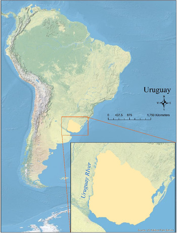
Tourism is important for Uruguay’s economy, representing 8.6 % of gross domestic product (GDP) in 2017 and generating 114,287 jobs which is approximately 6.3 % of total employment (Ministerio de Turismo, 2018). Tourism’s contribution to GDP has been on the rise since 2014 and is expected to continue to grow by 4.0 % per year until 2028 (WTTC, 2019). In 2018, Uruguay received 3.7 million tourists with 28 % visiting the capital Montevideo as their primary destination and 20 % visiting the sun and sand destination of Punta del Este. Tourism expenditure was over US$2.0 billion, with 41 % of this expenditure taking place in Punta del Este and 28 % in Montevideo (Ministerio de Turismo, 2018, 2019). This geographical concentration of tourism is one of the motives for the investment loan analyzed in this article, which aims to geographically diversify the tourism opportunities in the country. The Uruguay River Corridor was selected specifically for its potential for enhancing nautical tourism as well as ecological tourism and cultural tourism opportunities (Moreda et al., Reference Moreda, Hintze, Banerjee, Valle, Levy, Rauschert, Salazar, Bachino and Maya2017). Figure 1 presents a map of Uruguay and the Uruguay River.
Map of Uruguay.

This article is organized as follows: Section 2 provides a literature review of CGE and CBA, and details of the methods. Section 3 discusses the integration of CGE with CBA. Section 4 presents the analytical approach, scenario design, results, and analysis. Section 5 provides a discussion and the conclusions of the article.
2 Overview of the literature
2.1 CGE analysis
In the analysis of large public investments or policies that are expected to impact multiple sectors and actors in an economy with dynamic effects, a dynamic CGE approach is powerful. CGE analysis captures important intersectoral, and backward and forward linkages, and the direct, indirect, and induced benefits of an investment (Cattaneo, Reference Cattaneo2002; Dixon & Rimmer, Reference Dixon and Rimmer2002; Dwyer et al., Reference Dwyer, Forsyth and Spurr2003; Dwyer et al., Reference Dwyer, Forsyth and Spurr2005 ; Banerjee et al., Reference Banerjee, Cicowiez and Gachot2015). Pearce et al. (Reference Pearce, Atkinson and Mourato2006) suggest that where projects are large and complex, partial equilibrium frameworks are seldom sufficient and that the analytical framework should be capable of considering a wide range of impacts on all sectors that may be impacted. All project spillovers and indirect costs and benefits should be accounted for. A core strength of the CGE approach is its meticulous detail in appraising spillovers of an intervention (Pearce et al., Reference Pearce, Atkinson and Mourato2006).
Ex ante economic impact analysis with CGE models has been applied to public investments in the forestry (Banerjee & Alavalapati, Reference Banerjee, Alavalapati, Kant and Alavalapati2014; Banerjee et al., Reference Banerjee, Alavalapati and Lima2016a, Reference Banerjee, Cicowiez, Horridge and Vargas2019) and tourism sectors (Taylor, Reference Taylor2010; Taylor & Filipski, Reference Taylor and Filipski2014; UNWTO, 2014; Banerjee et al., Reference Banerjee, Cicowiez and Gachot2015, Reference Banerjee, Cicowiez and Cotta2016b, Reference Banerjee, Cicowiez, Morris and Moreda2018). Indeed, CGE analysis can be applied across a broad range of economic sectors where large public investments are concerned and intersectoral linkages are important. Beyond consideration of economic impacts of public investments, CGE models have a long history in applied policy analysis, from fiscal to trade to environmental policy analysis, with CGE models distinguishing themselves as the “workhorse” of policy analysis (Jones, Reference Jones1965; Dixon et al., Reference Dixon, Parmenter, Powell and Wilcoxen1992; Dixon & Jorgenson, Reference Dixon and Jorgenson2012). As Nobel Economist Kenneth J. Arrow stated: “…in all cases where the repercussions of proposed policies are widespread, there is no real alternative to CGE” (Arrow, Reference Arrow, Kehoe, Srinivasan and Whalley2005, p. 13).
CGE models are mathematical models that consist of systems of equations, which describe the relationships between sectors, agents, and other accounts in the underlying Social Accounting Matrix (SAM). CGE models are based on SAMs for a country, region, or for all countries linked together through trade as in the Global Trade Analysis Project database (Aguiar et al., Reference Aguiar, Narayanan and McDougall2016). A SAM provides a snapshot of an economy describing all monetary transactions between economic sectors and its agents, including households, government and enterprises, and the relationships between the modeled economy and other countries or regions of the world (King, Reference King, Pyatt and Round1985; Pyatt & Round, Reference Pyatt and Round1985).
A SAM is constructed based on a country’s System of National Accounts (European Commission et al., 2009) including integrated economic accounts, fiscal accounts and balance of payments data, and often government survey data such as household income and expenditure surveys. Recently, with the publication of the first international standard for environmental statistics, the System of Environmental-Economic Accounting Central Framework (European Commission et al., 2012), it has become possible to integrate detailed environmental information into CGE models. The development of the Integrated Economic-Environmental Modelling (IEEM) Platform has important applications for tourism investment analysis where tourism demand is a function of natural capital stocks and environmental quality (Banerjee et al., Reference Banerjee, Cicowiez, Horridge and Vargas2016c, Reference Banerjee, Cicowiez, Horridge and Vargas2019b).
CGE models are commonly used to assess economic impact and as such, some of the key indicators reported are GDP or gross regional product. As policy makers are frequently concerned with household income, consumption, and employment, these metrics are also often reported. In developing country contexts, indicators of poverty and inequality are frequently of interest, although disaggregation of households is necessary to generate meaningful results.
Indicators of changes in household welfare measured by compensating and EV may also be estimated in a CGE framework (Lofgren et al., Reference Lofgren, Harris, Robinson, Thomas and El-Said 2002). Where an intervention does not occur, EV is the amount of income an individual would have to be given to make them as well off (i.e., with the same level of utility) if the intervention did not take place.
Of course, where trade and fiscal policy shocks are the subject of analysis, impacts on exports, imports, the exchange rate, and levels of tax revenue become more relevant. With detailed representation of the environment in integrated modeling frameworks such as the IEEM Platform, measures of wealth such as genuine savings and inclusive wealth may also be reported (Stiglitz et al., Reference Stiglitz, Sen and Fitoussi2010; Arrow et al., Reference Arrow, Dasgupta, Goulder, Mumford and Oleson2012; Banerjee et al., Reference Banerjee, Cicowiez, Vargas and Horridge2019c).
2.1.1 Dynamic CGE model methods
Our CGE model combines a relatively standard recursive dynamic CGE model (see, for example, Robinson, Reference Robinson, Chenery and Srinivasan1989; Lofgren et al., Reference Lofgren, Harris, Robinson, Thomas and El-Said 2002), with additional equations and variables that can single out (i) domestic and foreign tourism demand; (ii) different modalities of tourism supply and demand; and (iii) the impact of public capital investment in infrastructure on sectoral productivity.Footnote 1 Supplementary Information for this article presents a non-technical overview mathematical statement of our model. Compared to other CGE models, this model combines policy-relevant features for the study of tourism investment or policy counterfactual scenarios in an economy.
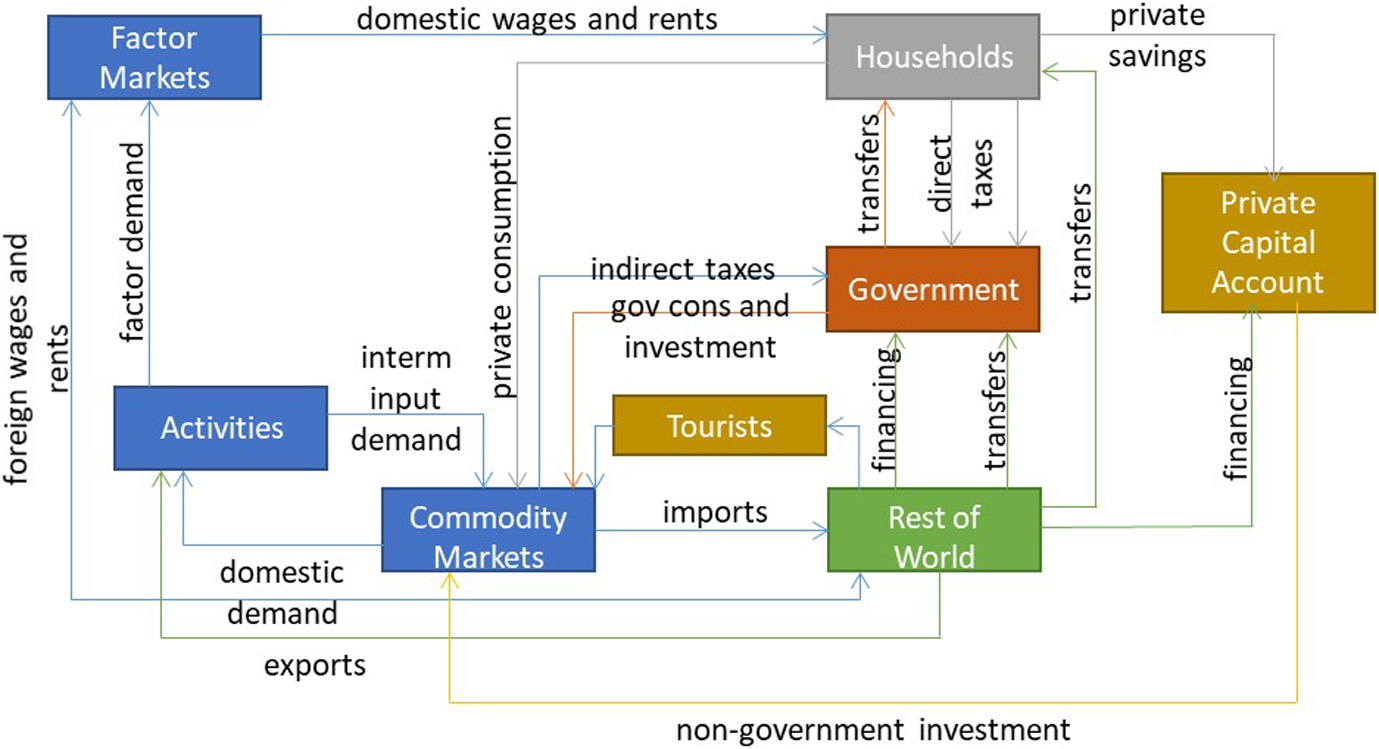
The major building blocks of a CGE model may be organized into activities which produce goods and services, markets for goods and services, markets for factors of production (labor, capital, land, and other natural resources), and three institutions, namely households, government, the rest of the world, and foreign tourists ( Figure 2).
Circular income flow in the CGE.

Activities produce goods and services, and sell their output at home or abroad and use their revenues to cover their costs of intermediate inputs, factor costs, taxes, and transfer what remains to investors as investment returns. Profit maximization drives firm decisions on levels of activity and factor use. Output of goods and services are exported and sold domestically depending on the relative prices of the output in world and national markets. For any exported commodity, exporters face either (i) export prices (free on board prices) that are exogenously determined, in which case export demand is infinitely price-elastic; or (ii) price-sensitive export demands which are defined by constant-elasticity functions with the free on board export prices linked to domestic conditions including the costs of production and the real exchange rate.
Households earn incomes from factors and transfers, which are used for consumption, direct taxes, and savings. Household consumption decisions vary in response to income and price changes. The household budget constraint ensures that the consumption value of the households equals their income net of direct taxes and savings.
The government receives receipts from taxes and transfers and uses these for consumption, transfers to households and investment. The government draws on the loanable funds market for supplementary funding, which is the case of the public investment in tourism considered in this article. To remain within its budget constraint, the government either adjusts its spending on the basis of available receipts or mobilizes additional sources of income through increasing taxes or foreign borrowing.
The rest of the world sends foreign currency to the modeled country in the form of transfers to its government and households, which in turn use these inflows to finance its imports. It is assumed that the balance of payments clears through adjustments in the real exchange rate, influencing export and import quantities and values in foreign currency. The private capital account provides investment financing from savings by households and the rest of the world, net of government financing.
Tourism demand from the rest of the world is modeled as an exogenous volume. In turn, total tourism demand is disaggregated across locally produced commodities using fixed coefficients. In the CGE model applied in this study, only foreign tourists are singled out. To do so in the SAM, an institution is added which represents foreign tourist expenditure in Uruguay. It is assumed that foreign tourists have a consumption basket that is based on fixed shares.
In domestic commodity markets, flexible prices ensure balance between demand and supply. Import prices in most cases would be exogenous, but the assumptions of the model can be adjusted for cases where import prices are endogenous. The share of imports in the national market is determined by import product prices relative to domestically produced product prices.
In factor markets, demand curves are downward-sloping reflecting the responses of production activities to changes in factor prices. In the case of labor, unemployment is endogenous. For each labor type, the model assumes an inverse relationship between the real wage and the unemployment rate (Blanchflower & Oswald, Reference Blanchflower and Oswald1994, Reference Blanchflower and Oswald2004). The model allows for different assumptions on labor mobility in response to wage differentials between the country and the rest of the world. For non-labor factors, the supply curves are vertical in any single year, that is, their quantity is fixed, but price adjusts according to the level of demand.
In our CGE, national income growth over time is endogenous. The economy grows due to the expansion of capacity determined by net fixed capital formation and labor availability as well as improvements in total factor productivity. The accumulation of private and government capital is through investment financed by local and external savings. Increased private capital is allocated across sectors according to their relative profitability. Once installed, capital becomes sector-specific and can only by adjusted through exogenously determined depreciation and the attraction of new investments.
2.2 CBA
The origins of CBA may be traced back to an application by U.S. Federal Water Agencies as early as 1808 where CBA was applied to evaluate the alternative use of public funds from an economy-wide perspective (Mishan, Reference Mishan1988; Burgan & Mules, Reference Burgan and Mules2001). Hanley and Spash (Reference Hanley and Spash1993) and Pearce et al. (Reference Pearce, Atkinson and Mourato2006) provide a brief history of the development of CBA. CBA is theoretically grounded in welfare economics where benefits are defined as increases in well-being or utility and costs are defined as reductions in utility. Thus, for an intervention to be welfare enhancing, the with-project social benefits must outweigh the social costs within a predefined geographic area.
There are two main aggregation rules that are often applied in CBA in estimating net impacts of an intervention. The first rule sums the willingness-to-pay for estimated benefits or the willingness-to-accept compensation for loss of benefits across a defined population. Willingness-to-pay and willingness-to-accept are at the core of welfare economics and correspond to compensating and EV. The second aggregation rule is applied in cases where it is appropriate to place a higher weight on the benefits or costs faced by different segments of the population such as the poor and more marginalized groups in society (Pearce et al., Reference Pearce, Atkinson and Mourato2006).
In applying CBA, the benefits accruing to a predefined population are estimated. When the population comprises several individuals or households, the benefits that would accrue to each household need to be aggregated to represent the overall benefits to the population. In other words, one needs to aggregate the individual impacts into a single impact. In doing so, different weighting schemes may be used to represent how the analyst assumes benefits will be distributed.
2.2.1 CBA methods
Following Hanley and Spash (Reference Hanley and Spash1993), CBA is conducted in seven main steps. The first step defines the project, identifies the resources to be used and for what purpose, and identifies the population expected to be affected by the intervention. The second step identifies project impacts where all resources used in the project including raw materials, capital, labor, land, and other resources are accounted for. The nature of the impacts will differ from project to project, although these impacts can range from impacts on income, output, prices, wages, and property value, to changes in environmental quality. Two important concepts in the identification of impacts are additionality and displacement. Additionality takes into consideration the marginal impact of the intervention while displacement is concerned with the reallocation of resources from an existing use, to the new intervention. Both concepts are critical in how results of the analysis are presented and interpreted.
The third step involves judgment on selection of the impacts that are economically relevant. With welfare economics underpinning CBA, the goal is to maximize a social welfare function. This function is estimated as the weighted sum of the utility of each individual in the population. In this context, utility is understood as the value of the consumption of marketed and non-marketed goods and services. A CBA should provide a decision rule for policy makers, enabling them to select the intervention that provides the greatest social utility.
The fourth step involves physical quantification of the economically relevant impacts while the fifth step is the monetary valuation of these impacts. Ascribing a monetary value to non-market goods can be challenging, although methods for doing so are continually becoming more robust. These methods are categorized as revealed preferences and stated preferences. Revealed preferences include direct methods such as damage cost and replacement cost, and indirect methods such as hedonic and random utility approaches (Pearce et al., Reference Pearce, Atkinson and Mourato2006). Stated preference approaches include contingent valuation and choice modeling; these stated preference methods are the primary approach for estimating non-use values (Champ et al., Reference Champ, Boyle and Brown2003; Pearce et al., Reference Pearce, Atkinson and Mourato2006; Johnston et al., Reference Johnston, Boyle, Adamowicz, Bennett, Brouwer, Cameron and Hanemann2017). Where ascribing a monetary value to non-market goods and services is not feasible or desirable, economic measures may be supplemented by biophysical ones (Stiglitz et al., Reference Stiglitz, Sen and Fitoussi2010; Polasky et al., Reference Polasky, Bryant, Hawthorne, Johnson, Keeler and Pennington2015).
The sixth step of the analysis applies the net present value (NPV) test, which assesses whether the sum of discounted benefits exceeds the sum of discounted costs. If the result is positive, the intervention is considered an efficient allocation of resources. Calculation of NPV involves making a decision on the rate of time preference or discount rate, and discounting the flow of costs and benefits, converting all values to present value terms.Footnote 2 This calculation is shown in Equation (1).
 $$ \mathrm{NPV}=-{I}_0+\frac{C_1}{1+r}+\frac{C_2}{{\left(1+r\right)}^2}+\cdots +\frac{C_T}{{\left(1+r\right)}^T}, $$
where NPV is net present value,
 $ {I}_0 $
is the initial investment,
 $ T $
is the final year of the period of analysis,
 $ C $
is the cash flow, and r is the discount rate.
The seventh and last step in a CBA is to undertake sensitivity analysis to assess which parameters have the strongest effect on NPV. Usually, the parameters tested in the sensitivity analysis are the physical quantities and qualities of inputs and outputs, prices, and in some cases, the discount rate and project time horizon.
3. Integration of CGE and CBA
Public investment in tourism can be motivated by the impact the investment is expected to have on income and employment, which are enhanced by increased tourism expenditure in a region. In developing country contexts, reducing poverty and inequality as well as reducing regional disparities can also drive public investment. Government investments may also be directed to correcting market failures when individual tourism sector firms are unable to capture the share of tourist expenditure that is commensurate with their expenditures and promotional, and organizational efforts (Burgan & Mules, Reference Burgan and Mules2001). Where investment is justified based on its expected benefits, it is important to define benefits precisely.
From a CBA perspective, benefits equate with welfare and the net benefit is the change in welfare, net of the real resource costs. Defining benefits as increases in tourist expenditure and evaluating these in a CBA would not be consistent with the welfare economics foundation of CBA. In an economic impact assessment framework, evaluation of the economic benefits in terms of tourism expenditure or regional product may be appropriate, although these indicators are not valid measures of benefits from a welfare economics standpoint.
As discussed in Dwyer et al. (Reference Dwyer, Jago and Forsyth2016) and Abelson (2011), while an investment with a positive impact on GDP may be welfare enhancing, GDP alone suffers from a number of limitations as a measure of welfare. GDP measures the value of all economic output. From the income approach to calculating GDP, this includes the income earned by non-resident owners of capital and non-resident labor and as such, accounts for benefits that accrue outside of the region of interest. Second, interpreted from the expenditure approach to calculating GDP, an increase in GDP can be driven by measures to mitigate additional reductions in welfare. For example, expenditure to clean up an oil spill or remove plastic waste from oceans would be recorded as positive contributions to GDP. Furthermore, while GDP captures income or expenditure flows, it does not provide indications of the sustainability of these flows (Stiglitz et al., Reference Stiglitz, Sen and Fitoussi2010; Lange et al., Reference Lange, Wodon and Carey2018).
In a partial equilibrium framework, to be compatible with the welfare underpinnings of CBA, the appropriate metrics of benefits are consumer or producer surplus. In the case of tourism, however, and particularly when enhancing foreign tourism expenditure is the aim, consumer surplus is not the appropriate indicator of welfare since the consumer is a foreign visitor. Although enhancing the foreign visitor experience is important for increasing tourism revenue, the Government’s primary policy objective will be to improve the welfare of its constituents and thus the benefits that accrue to residents of their jurisdiction, rather than the benefits perceived by individuals residing elsewhere. In a partial equilibrium framework, the relevant metric for welfare from a public policy standpoint is producer surplus where benefits to the economy are assessed as a function of increases in local production (Burgan & Mules, Reference Burgan and Mules2001).
A general equilibrium framework enables consideration of public policy and investment on households. In this framework, household welfare or utility is the appropriate measure of benefits and is readily estimated in a CGE framework (Hanley & Spash, Reference Hanley and Spash1993; Blake, Reference Blake2005; Pearce et al., Reference Pearce, Atkinson and Mourato2006; Dwyer et al., Reference Dwyer, Jago and Forsyth2016). As pointed out by Dwyer et al. (Reference Dwyer, Jago and Forsyth2016), EV translates an estimate of economic impact into a welfare measure based on assumptions made with respect to factor mobility and constraints. The CGE approach has additional advantages over partial equilibrium frameworks since the impacts of second and subsequent rounds of direct, indirect, and induced impacts generated by an investment are also captured. Furthermore, the CGE approach affords a level of internal consistency not possible in a partial equilibrium framework by balancing supply and demand for goods, services, savings, and investment and factors, subject to resource constraints.
Model assumptions on factor mobility and constraints are important considerations in interpreting net benefits estimated through a general equilibrium and a conventional partial equilibrium CBA approach. In a general equilibrium setting, if labor and capital are diverted from an existing use to a new intervention, the net benefit would only be positive if the new use generated greater welfare. A partial equilibrium approach, however, would not account for this resource diversion and thus could lead to an overestimation of net benefits. The use of estimates of welfare impacts generated through a general equilibrium approach in a CBA overcomes this limitation. This the method developed in the section that follows.
Another important consideration in both a general equilibrium and CBA framework is the opportunity cost of labor. When the opportunity cost of labor is equal to zero, the social benefit of an additional job is the wage paid to the new salaried worker. Where unemployment exists and the opportunity cost (i.e., the unemployed workers’ reservation price) is less than the minimum wage, the benefit of the additional job is the difference between the minimum wage and the worker’s reservation price (Bartik, Reference Bartik2012). In areas with high unemployment, few social safety nets and where labor is mobile between sectors and regions, it may be reasonable to assume that the opportunity cost of the unemployed worker is very close to zero. In developing country contexts, this is often the case.
Layman (Reference Layman2004) argues that for the results of general equilibrium analysis to provide meaningful information to policy makers, a recognized set of methods, assumptions, and indicators are required. For example, any additional resources used in an intervention should be accounted for and the costs associated should be deducted from gross product (Hanley & Spash, Reference Hanley and Spash1993; Layman, Reference Layman2004). Indeed, one of the strengths of the CGE approach is that it is an internally consistent framework providing a strict accounting of all market costs and benefits generated by an intervention. With increasing experience in applying CGE to public investment analysis, methods, assumptions, and indicators are becoming increasingly standardized (UNWTO, 2014; Banerjee et al., Reference Banerjee, Cicowiez, Morris and Moreda2018; Banerjee & Cicowiez, Reference Banerjee and Cicowiez2019).
Although CBA has a long history of incorporating non-market benefits in the analysis, recent efforts have improved non-market considerations in CGE analysis. Integration of non-market benefits can be achieved through the use of outputs from specialist models in a CGE and through linking different specialist models with CGE. For example, Dixon et al. (Reference Dixon, Rimmer and Waschik2017) use the outputs of a highway investment model to estimate impacts of increasing highway expenditures. The Highway Economic Requirements System model was used to estimate impacts on vehicle operating costs, travel time, and other key variables, which were later used in a CGE model to derive results for indicators such as GDP, employment, and welfare. Other work by Banerjee et al. (Reference Banerjee, Cicowiez and Dudek2019a) links the IEEM Platform with ecosystem services modeling (IEEM + ESM), which enables the estimation of the contribution of ecosystem services to economic outcomes. For example, Banerjee et al. (Reference Banerjee, Cicowiez and Dudek2019a) estimate how changes to erosion mitigation ecosystem services affect agricultural and livestock productivity, which in turn impact the overall level of economic output and growth.
4 Integration of CGE and CBA: An application to Uruguay
This section applies a CGE approach to assessing the impacts of a public investment in tourism in Uruguay and uses the results in a CBA framework. The CBA is presented from the perspective of a multilateral development bank and from the perspective of the beneficiary government. From the development bank’s perspective, on the cost side, what is of concern is the disbursement schedule of the loan. On the benefit side, the development bank is interested in increasing net social benefits for the borrowing country. From the perspective of the borrowing country, on the cost side, the government is concerned with the repayment schedule of the loan. On the benefits side, as with the development bank, the government also seeks to maximize the net social benefits accruing to its citizens. Based on the discussion above, and since we are concerned with changes in welfare of the citizens of the borrowing country, EV is the appropriate measure of welfare and it is the indicator used in the CBA.
The CGE model developed in Banerjee et al. (Reference Banerjee, Cicowiez and Gachot2015, Reference Banerjee, Cicowiez and Cotta2016b) and described in subsection 2.1.1 is calibrated with a new SAM for Uruguay with a base year of 2013 (Cicowiez, Reference Cicowiez2016). The CGE is applied to the ex ante economic analysis of a US$6.25 million public investment in tourism. This investment is supporting tourism development in the Uruguay River Corridor to create employment and income in emerging destinations and consolidate tourism opportunities to improve regional equity.
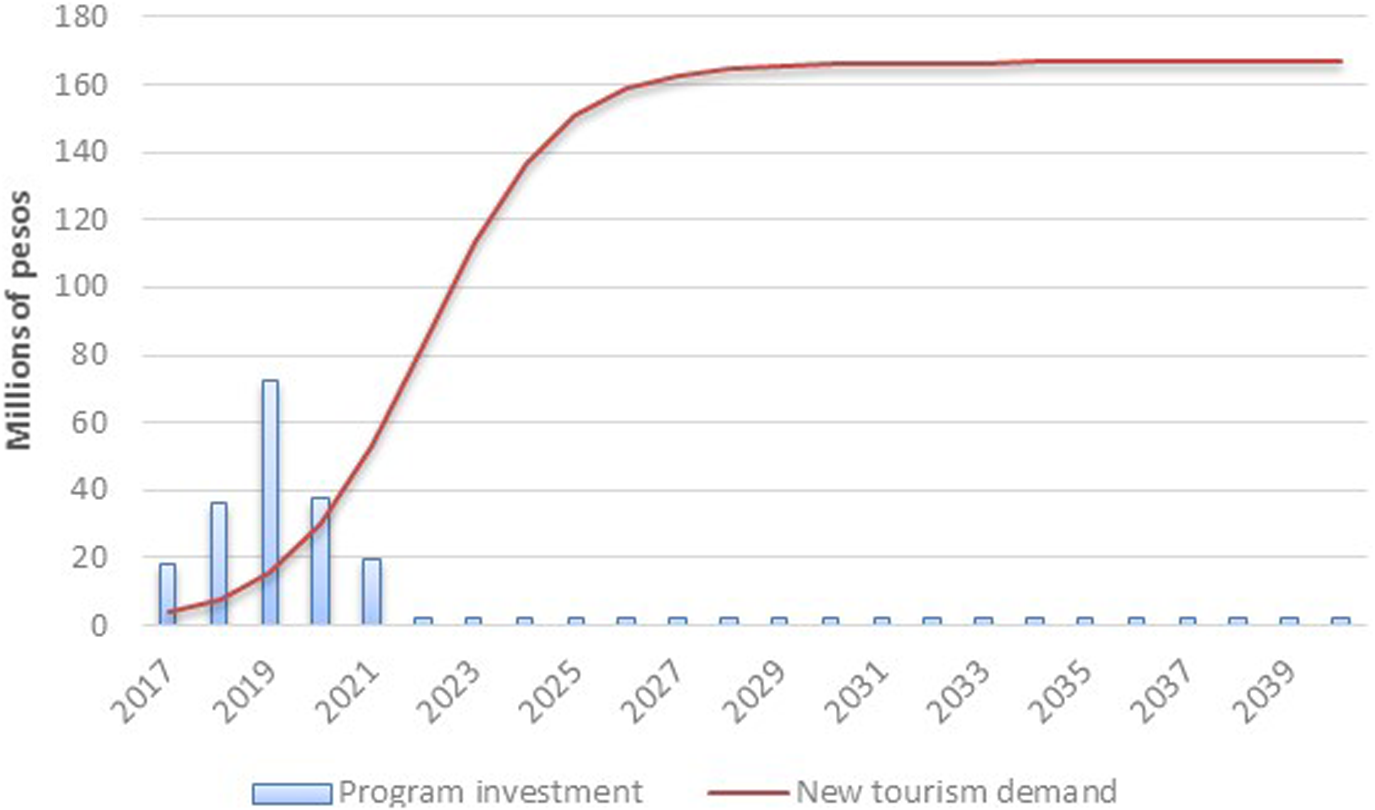
The three main objectives of the investment are to (i) create and consolidate tourism infrastructure (US$3.555 million); (ii) catalyze private sector investment in the corridor (US$950,000); and (iii) strengthen regional tourism governance (US$900,000). Operations and maintenance of new infrastructure is estimated at an annual cost of 3 % of the value of this infrastructure. Management costs of the tourism program are accounted for during the first 5 years and total US$845,000. This amount is applied proportional to the amount of infrastructure investment in the first 5 years. Figure 3 describes the distribution of the investment and operations, and maintenance costs until 2045, which is the time horizon used in this analysis.
Distribution of investment costs and projected tourism demand increase.

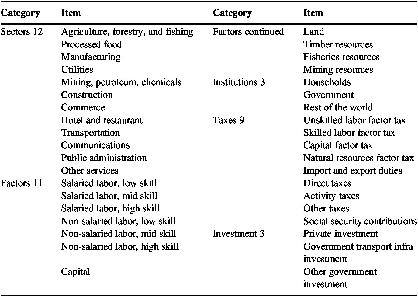
Table 1 describes the accounts in the Uruguay SAM. The SAM developed was extended to disaggregate foreign tourism demand.
Main accounts in the Uruguay SAM.

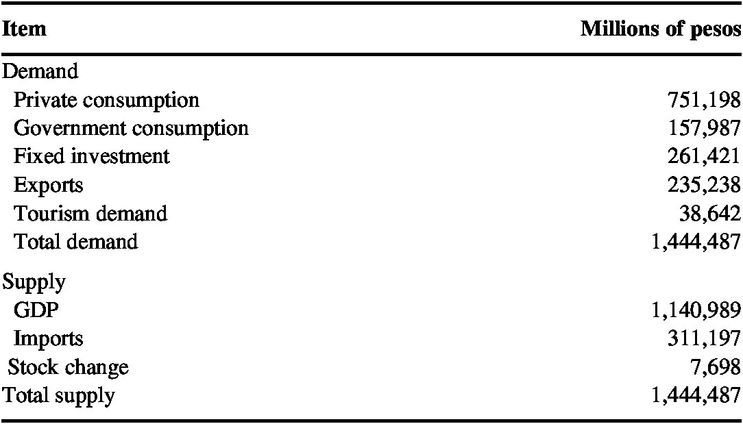
According to the SAM, Uruguay’s GDP reached 1,140,989 million pesos in 2013. Uruguay imported 75,958 million pesos more than it exported, while foreign tourism demand directly contributed to almost 3.4 % of GDP ( Table 2).Footnote 3
Uruguay, 2013, total supply and demand.

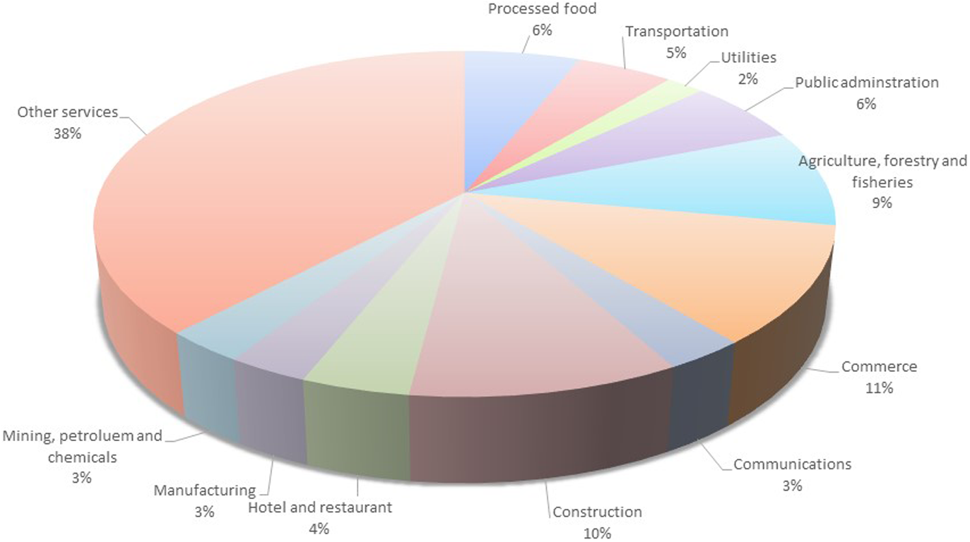
The sectoral structure of Uruguay’s economy is depicted in Figure 4. The Other services sector is the largest sector accounting for 38 % of the economy’s value added. Commerce is a far second followed by Construction, and then Agriculture, forestry, and fisheries. Although not shown here, Processed food and Agriculture, forestry, and fisheries lead Uruguay’s exports (35 % and 28 %, respectively). The Manufacturing and the Mining, petroleum, and chemicals sectors account for the greatest share of imports.
Sector structure in 2013, value added shares.

4.1 Scenario design
The following five scenarios were undertaken: (i) the baseline scenario that is the without investment scenario (baseline). This is the baseline to which all other scenarios are compared; (ii) the investment scenario where the government investment in tourism infrastructure, institutional strengthening, and capacity building is implemented (invest); (iii) the demand scenario, which simulates the projected increase in foreign overnight leisure tourism expenditure arising from the investment (demand); (iv) a combination scenario where the investment and demand scenarios are implemented jointly (combi); and (v) a final scenario, which is the combi scenario with the internalization of the repayment of the US$6.25 loan in the CGE simulation (combi-pay). Details of each scenario are as follows.
4.1.1 Baseline scenario
This baseline scenario assumes that average past trends will continue from 2014 to 2045. The non-base scenarios that follow only deviate from the baseline scenario beginning in 2017.
4.1.2 Invest scenario
The invest scenario imposes increased government investment in tourism infrastructure, institutional strengthening, and capacity building financed through a multilateral development loan. The investment schedule is shown in Figure 3. The year 2017 is the first year of the investment, which continues until 2021, inclusive. The investment itself includes technical studies; interpretive touristic circuits; investments in enhancing cultural and ecological assets, and visitor’s centers; a tourism statistics, information and marketing system; and tourist operator capacity building and a local competitive tourism development fund. Figure 3 also shows annual operations and maintenance costs of new infrastructure (3 % of the value of new infrastructure per year) as well as infrastructure management costs equal to US$845,000 annually (Moreda et al., Reference Moreda, Hintze, Banerjee, Valle, Levy, Rauschert, Salazar, Bachino and Maya2017). The investment enters the CGE model from the rest of the world as foreign financing to the government ( Figure 2), which is in turn used for the purchase of goods and services according to the composition of the investment.
4.1.3 Demand scenario
In the demand scenario, foreign leisure overnight tourist arrivals and expenditure are projected to increase as a result of the increased tourism opportunities created by the investment. With program tourism demand was estimated in Eugenio-Martin and Inchausti-Sintes (Reference Eugenio-Martin and Inchausti-Sintes 2016) with econometric regression analysis. In this regression, the economic value of the presence of an additional tourism attraction was estimated using tourism expenditure as the independent variable. The three attractions considered were nautical tourism, ecotourism, and cultural tourism attractions.
Based on the characteristics and number of new attractions to be developed through the investment, the total additional tourism expenditure was estimated at over 166 million pesos. This increased tourism demand was distributed according to a logistical functional form, which represents a gradual increase over time until the point of inflection after which growth in tourism demand attributable to the investment begins to slow. This increase in growth is applied over a 14-year period such that the new tourism demand reaches 50 % in year 2022 and 100 % in 2030 ( Figure 3).
4.1.4 Combi scenario
The combi scenario models the invest and demand scenarios combined.
4.1.5 Combi-pay scenario
The combi-pay scenario models the invest and demand scenarios combined and internalizes the repayment of the US$6.25 million loan in the CGE model. According to conditions applied to similar multilateral loans, repayment begins after a grace period in year 7, which is year 2023 in this analysis. Interest owing and the principal payment are made annually with the final payment made in 2039. The interest rate used is 1.58 % and is based on the US Dollar LIBOR.Footnote 4 The value of the repayment is held constant over the period and is equivalent to 11.85 million Uruguayan pesos.
To finance repayment of the loan, the household income tax rate is adjusted to generate the necessary funds. The mechanics of this repayment in the CGE are as follows. In the dataset and CGE, there is a single representative household. In order to clear the government budget, the household income tax rate scales up or down endogenously to generate sufficient government revenue to finance its expenditure.
Model closure rules are required to determine the mechanisms by which demand and supply are equalized in all markets. In this analysis, government consumption is kept as an exogenous variable and is not adjusted to balance the budget. Instead, in non-base scenarios, government foreign borrowing is adjusted to finance the public investment in tourism. That is, the government borrows from the rest of the world to finance the increase in public investment, which is consistent with a situation in which a country borrows capital from a multilateral development bank. Private investment is savings-driven. Foreign borrowing to finance the non-government capital account is kept fixed at its baseline value expressed in foreign currency units. The real exchange rate balances the current account of the balance of payments.
In the case of labor, unemployment is modeled with a wage curve calibrated using recent estimates for the elasticity of wages with respect to the unemployment rate; specifically, its value is −0.1 (Anaya & Rodríguez-Villamil, Reference Anaya and Rodríguez-Villamil 2012). For capital, we assume that once installed, capital is immobile and cannot move to different sectors. This assumption was made to reflect that capital differs according to the sector that uses it. The consumer price index is the numeraire.
In addition to model closure rules, elasticities and other free parameters also influence the results of CGE simulations. Elasticities inherently have an estimation error. To understand the implications of this estimation error, systematic sensitivity analysis was conducted to evaluate the robustness of the results with respect to model elasticities. Detailed results of this analysis are presented in the Appendix.
4.2 CGE model results and analysis
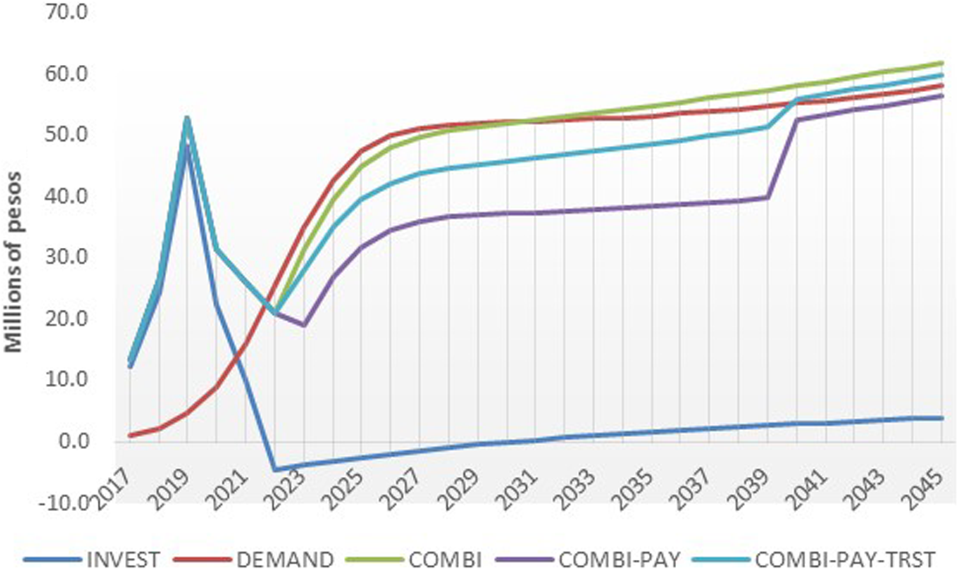
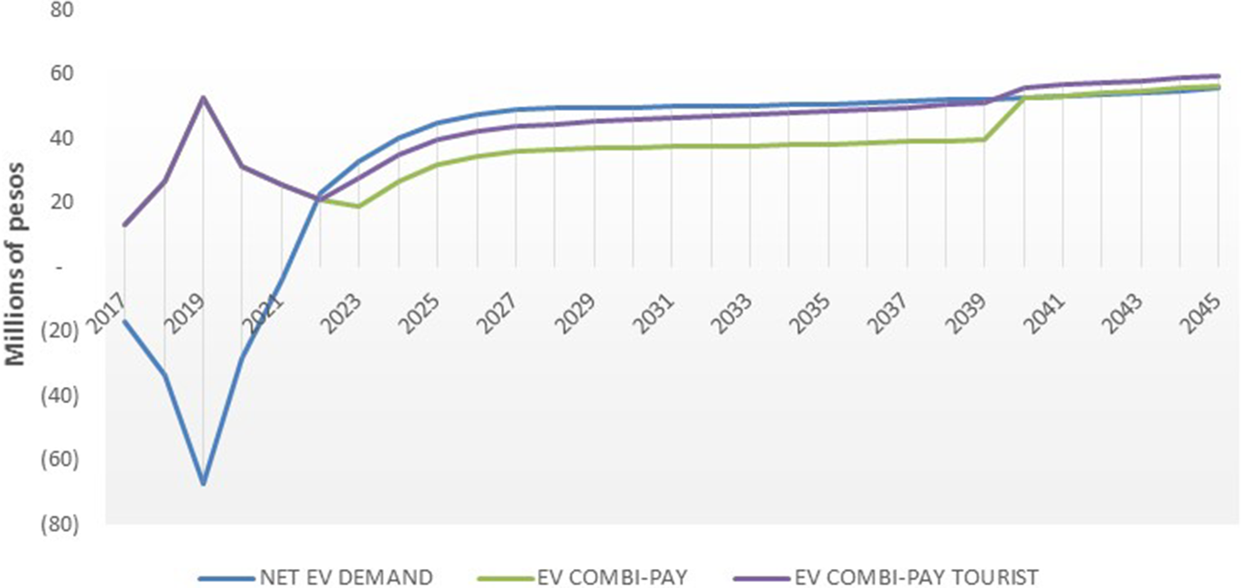
Figure 5 illustrates impacts on household welfare measured by EV in millions of pesos. EV represents the amount of income an individual would have to be given to make them as well off (i.e., with the same level of utility) as they would be if the intervention did take place. In the invest scenario, EV spikes with the disbursements of the loan reaching a maximum in 2019. After 2019, EV falls toward baseline levels and dips below the baseline in 2022. During the 5-year period in which the public investment is implemented, there is a temporary crowding out of private investment due to increase capital costs, which has a negative impact on EV. At the same time, increased economic activity generates greater household income and savings, which results a net positive impact on EV.
Impact on equivalent variation, deviation from baseline, millions of pesos.

The impact on EV in the demand scenario closely follows the increase in projected demand from the creation of new tourism attractions and opportunities. This increase in EV is driven by a reduction of unemployment and an appreciation of the real exchange rate, which also has a positive effect on household consumption, making imported goods relatively cheaper. The combi scenario is the joint impact of the invest and demand scenarios. The contribution of the demand scenario offsets the small negative impact that was perceived in the invest scenario around 2022 and the trend is positive throughout the period of analysis. By 2045, EV is an additional 60 million pesos above baseline levels.
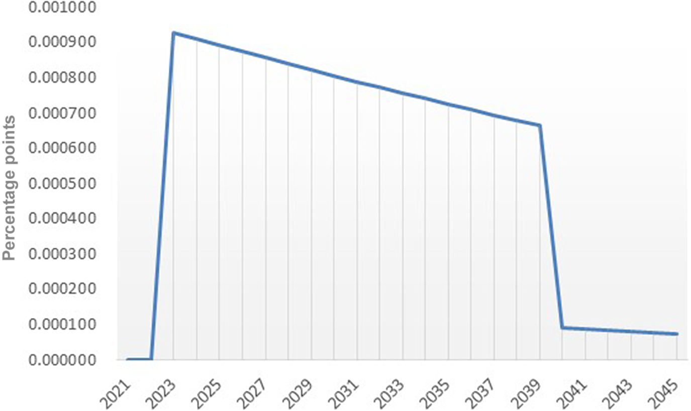
The combi-pay scenario follows a similar trend as the combi scenario, although the combi-pay trend is between 5 and 15 million pesos lower than the combi scenario during the loan repayment period. EV in combi-pay remains lower due to the higher direct tax rate and corresponding lower savings. As a result of the higher direct tax rate and lower savings, private capital stock decreases relative to the combi scenario during the loan repayment period. Household income tax differs between combi-pay and combi by 0.000927 % in 2023 and falls slowly until 2039 after which most of the loan is repaid ( Figure 6). From 2040 onward, the household tax rate adjusts back downward to 0.00091 %, remaining relatively stable thereafter. These small adjustments in the tax rate are consistent with the size of the loan relative to the size of the Uruguayan economy and tax base.
Difference from baseline in household tax rate, percentage points.

In combi-pay, EV spikes upward in 2039 once the loan is repaid, although remains below combi levels due to the forgone increase in capital stock resulting from loan repayment. In 2045, the difference between the combi and the combi-pay scenario is 5.3 million pesos. The cumulative difference in EV between the combi and combi-pay scenario by 2045 is almost 289 million pesos.
As discussed in subsection 4.1, model elasticities influence the results of CGE analysis. To understand the implications of inherent elasticity estimation errors, systematic sensitivity analysis was conducted (Appendix). Results of this analysis confirm the robustness of the results presented here showing that in the case of the combi scenario, there is virtual certainty that household welfare would increase with the public investment in tourism.
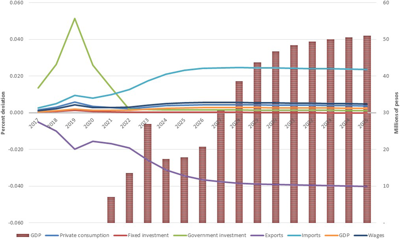
Figure 7 shows how key macroeconomic variables evolve over time in the combi scenario. Exports (which exclude foreign tourism spending) are below baseline levels due to slightly reduced output from export sectors. This is also the consequence of the real exchange rate appreciation. In fact, the tradable sector suffers a kind of Dutch disease due to the increase in the spending of foreign tourists. The exchange rate appreciation enables households to consume more imports. Wages, private consumption, government investment, and GDP are all above baseline levels in combi. GDP in 2045 is 55 million pesos above the baseline. Although not shown here, private fixed investment is lower than the baseline during the public investment stimulus. This is the result of a temporary crowding-out effect that is caused by the increase in public investment and the consequent increase in the price of capital goods, which is a feature that has been identified in similar analysis (Dwyer et al., Reference Dwyer, Forsyth and Spurr2005; Banerjee et al., Reference Banerjee, Cicowiez and Cotta2016b).
Evolution of macroeconomic indicators in present deviation from base (left axis) and millions of pesos (right axis).

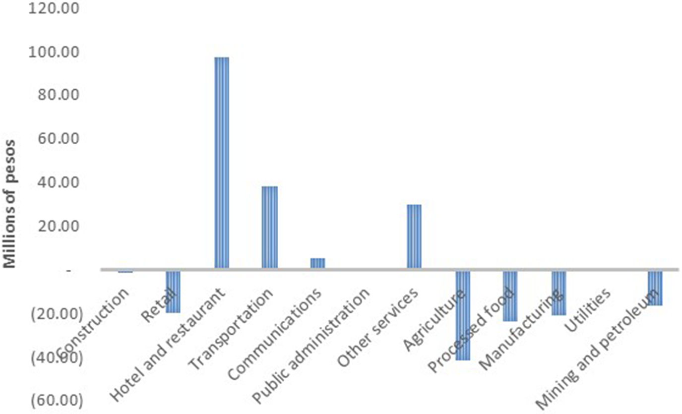
In terms of sectoral results, the Hotel and restaurant sector is strongly stimulated by 98 million pesos by 2035 relative to the baseline ( Figure 8). Other gainers are the Transportation sector and Other services sector. Some sectors contract in response to the investment and these are primarily comprised of the Agricultural sector, followed by the Processed food and Manufacturing sectors. Reduced output from these sectors contributes to the slower growth in Uruguayan exports arising from the public investment. It is important to note that much of these changes are small, although consistent with the size of the investment shock.
Value added growth, deviation from BASE in 2035, millions of pesos.

Finally, an alternative approach to financing the repayment of the loan is considered. Although combi-pay adjusts the household tax rate to finance loan repayment, we consider instead a levy of a new tourist tax to collect the additional resources for loan repayment. Results show that taxing foreign tourism dampens the impact repayment has in the combi-pay scenario where repayment is financed through taxing household income (see COMBI-PAY-TRST in Figure 5). The tourist tax is on average 0.01 % between 2023 and 2034 and is levied on total foreign tourist expenditure. A key assumption explaining this result is that foreign tourist demand is exogenous in the scenarios and thus tourists do not respond to the imposition of the new tax. With a tax of this magnitude, this may be quite a reasonable assumption with the tax not really factoring in to tourists’ decisions to visit the destination.
4.3 CBA
In this section, the investment is considered from the perspective of a multilateral development bank and from the perspective of the beneficiary government. It is important to note that a multilateral development bank is a non-commercial lender and thus it is not driven by a profit motive but rather one related to improving the welfare of the beneficiary country while meeting its basic operational costs. Equation (2) shows that from the perspective of the lender, the NPV of the investment is calculated by (i) calculating the EV from the demand scenario, which is the estimated national welfare impact of the change in tourism demand [term two in Equation (2)]; (ii) summing this term with the cost of the investment incurred, in this case during the first 5 years; (iii) adding this term with the future repayment of the loan which begins following the grace period of 6 years; and (iv) discounting the calculated values for each year back to the current year.
The EV from the demand scenario is used as the measure of welfare since it would not be conceptually correct to use the EV from combi or combi-pay because they both consider the investment in the calculation of EV. The inevitable disadvantage of this is that the general equilibrium impacts of the investment are not considered in the estimation of EV from the lender’s perspective. Should it be possible to consider these general equilibrium impacts, the welfare impacts would generally be greater.
Another feature to note is that in order to calculate an internal rate of return (IRR), it is necessary for there to be at least 1 year of negative cash flow. In Equation (2), this will be the case where in one or more of the first 5 years of loan disbursement, the amount of the loan disbursement is greater than the welfare benefit. We use the standard discount rate of 12 % used by some multilateral lenders such as the Inter-American Development Bank. With the cost of the loan perceived from the lender’s perspective in the first 5-years of the NPV analysis, these costs are weighted heavily.
Calculation of NPV from the lender’s perspective:
 $$ \mathrm{NPV}=\sum_{t=2017}^{2021}\frac{-L/5}{{\left(1+r\right)}}+\sum_{t=2017}^{2045}\frac{EV_t}{{\left(1+r\right)}^{2017-t}}+\sum_{t=2023}^{2039}\frac{L/17\left(1+i\right)}{{\left(1+r\right)}^{2023-t}}, $$
where L is the total amount of the loan, in this case divided by five, which is the disbursement period. EV is the change in welfare represented by EV from the demand scenario. The first term is the discounted loan issued over the disbursement period. The second term is the discounted welfare impact of the investment over the period of analysis. The third term is the discounted lender’s receipts of the loan repayment beginning in 2023 following a 6-year grace period in this case and terminating in 2039.
From the perspective of the beneficiary government, its concern is the welfare benefit generated by the investment and the future repayment of the loan. From this perspective, in almost all circumstances, cash flow will be positive for all years thus precluding the calculation of an IRR. NPV is calculated using the EV from the combi-pay scenario. Discounting this EV estimate yields the NPV of the investment considering general equilibrium impacts of the repayment of the loan. In other words, the second and subsequent round of impacts caused by the diversion of government resources to repay the loan are accounted.
Table 3 shows the results of the NPV analysis from both the multilateral lender and the beneficiary government’s perspective. With all direct costs incurred in the first 5 years of the period of analysis, the NPV from the lender’s perspective is 94 million pesos. NPV from the beneficiary government’s perspective is 282 million pesos. Also shown in Table 3 is the NPV of the investment considering loan repayment financed through a tourist tax rather than household income tax. In this case, NPV is the highest at 318 million pesos. Figure 9 shows the distribution of net benefits of time.
Net benefits calculated with EV from demand, combi-pay, and combi-pay tourist, millions of pesos.

Net present value and internal rate of return from the multilateral lender and beneficiary’s perspective; millions of pesos.

The NPV analysis undertaken from the beneficiary’s perspective results in a higher NPV than from the lender’s perspective. This is largely a function of the fact that costs from the lender’s perspective are incurred in the first 5 years of the analytical time horizon and thus are weighted heavily in the discounting exercise. From the beneficiary’s perspective, follow-on costs that may arise from the repayment of the loan are considered. Specifically, modeled in this way, just as CGE analysis accounts for first, second, and subsequent round impacts of increased economic activity, building the payment in to the CGE analysis also considers the multiple rounds of cost impacts due to forgone government expenditure with government resources allocated toward loan repayment. This is a distinct advantage of the approach presented here.
From the multilateral lender’s perspective, the investment results in an internal rate of return of 18 %. From the beneficiary’s perspective, it is not possible to calculate an IRR for the investment. The reason for this is that since no costs are incurred until 2023, there is no negative cash flow in the initial years of the investment. That it is not possible to calculate an internal rate of return from the beneficiaries perspective may not be an issue; however, since in practice, once an investment loan has been formulated, the CBA is often used to validate the economic viability of the loan rather than compare among investment opportunities which the main application of the IRR.
5 Discussion and conclusions
In this article, we draw on the strengths of CBA and CGE modeling and present a rigorous and integrated approach to evaluating the ex ante economic impacts of public investments in tourism. We undertake this analysis from the perspective of a multilateral development bank that provides loanable funds and from the perspective of the beneficiary government. An innovative feature of our approach is that in considering the beneficiary government’s perspective, we build-in the repayment of the loan into the CGE analysis and then estimate the NPV of the investment. An important advantage of this approach is that just as the first, second, and subsequent rounds of impacts of increased economic activity are considered in the analysis, it also considers the multiple rounds of impacts created by the diversion of government resources toward loan repayment. As such, our approach takes into consideration any forgone economic activity that may have arisen from reallocation of public budget resources toward the repayment of the loan.
For compatibility with the welfare economics foundations of CBA and the characteristics of public investment in tourism where the target beneficiaries are usually tax paying and voting households, EV is the appropriate measure of welfare and is readily estimated in a CGE framework. There are several strengths of the CGE framework for estimating benefits. First is its ability to capture first and subsequent round investment impacts on household welfare, on both the benefit and cost side. The ability to model household level impacts is a distinct advantage, which provides an attractive alternative to undertaking time consuming and costly household surveys which can be infeasible under the usually tight time and resource constraints characteristic of loan preparation periods faced by multilateral development banks. Second, the CGE approach estimates overall net benefits robustly by explicitly accounting for factor constraints and resource diversion. Third, a CGE model’s internally consistent accounting framework renders double counting of benefits and costs impossible.
The analysis of a US$6.25 million public investment in tourism in Uruguay was undertaken from the perspective of a multilateral development bank and the beneficiary government. Viewed from the perspective of the multilateral lender, with the cost to the lender incurred in the first 5 years, the NPV is lower than when compared with the NPV estimated from the perspective of the beneficiary government. This result is explained by the fact that costs incurred by the beneficiary government begin following a 6-year grace period, with repayment beginning in 2023. It is the distribution of these costs and the discounting of net benefits that results in the lower NPV from the perspective of the multilateral development bank.
Internalizing the repayment of the loan in the CGE analysis is more realistic than considering this repayment outside of the modeling framework. With the repayment internalized, public resources allocated to the repayment of the debt has implications for current government expenditure and thus has an opportunity cost associated with it. As shown in this application, despite this consideration of opportunity cost, the NPV of the investment was still higher when considered from the beneficiary government’s perspective because the costs were incurred further in the future when compared with the lender’s perspective.
For the purposes of ex ante economic analysis of multilateral development loans, one potential drawback of the approach is that, given the repayment schedule of the investment examined in this study, it was not possible to calculate an IRR from the beneficiary’s perspective. This, however, is only a limitation if the CBA is used to compare alternative investments, rather than explore, enhance transparency, and demonstrate the economic viability of a specific investment.
Supplementary Material
To view supplementary material for this article, please visit https://dx.doi.org/10.1017/bca.2019.32.
Appendix
A. 1 Sensitivity analysis of model elasticities
The results from a CGE model are a function of (i) the model structure, including functional forms used to model production and consumption decisions and macroeconomic closures; (ii) the database used for model calibration; and (iii) the values assigned to the model elasticities or, more generally, to the model’s free parameters. In other words, the elasticities used in this study implicitly carry an estimation error, as in any similar model. To better understand the implications of this, we performed a systematic sensitivity analysis of the results with respect to the value assigned to the model elasticities. Hence, if the conclusions of the analysis are robust to changes in the set of elasticities used for model calibration, we will have greater confidence in the results presented above.
In the systematic sensitivity analysis, it is assumed that each of the model elasticities is uniformly distributed around the central value used to obtain the results. The range of variation allowed for each elasticity is ±75 %, which represents a fairly wide range of variation for each model elasticity. Our method is a variant of the one originally proposed by Harrison and Vinod (Reference Harrison and Vinod1992). In short, the model is solved iteratively with different sets of elasticities. The resulting distribution of results is used to build confidence intervals for selected model results. The steps for the systematic sensitivity analysis are as follows:
-
(i) The distribution (i.e., lower and upper bound) is computed for each model parameter that will be modified, which are elasticities of substitution between primary factor of production, trade-related elasticities, expenditure elasticities, and unemployment elasticities for the wage curves.
-
(ii) The model is solved repeatedly, each time with a different set of elasticities following a Monte Carlo type procedure. First, the value for all model elasticities is randomly selected. Second, the model is calibrated using the selected elasticities. Third, the same counterfactual scenarios as previously described are conducted. These three steps are repeated 500 times, with sampling with replacement for the value assigned to the elasticities.
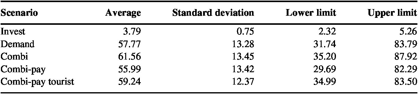
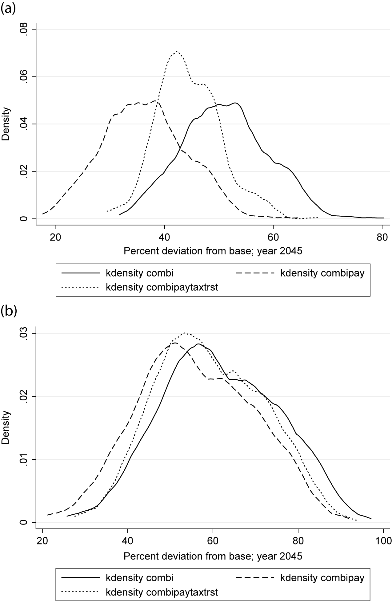
Table A1 shows the percentage change in EV in 2045 estimated (i) under the central elasticities and (ii) as the average of the 500 observations generated by the sensitivity analysis. For the second case, the upper and lower bounds under the normality assumption were also computed. All runs from the Monte Carlo experiment receive the same weight. As can be seen, the results for EV reported in the main text are significant and are within the confidence intervals reported in Table A1. For example, it is almost fully certain that the simulated combi scenario would have a positive effect on EV in the range between 35.2 and 87.9 million pesos. In addition, mean-comparison tests show that the increase in EV is significantly higher in the loan repayment with a tourism tax imposed than when loan repayment is financed through income tax.
Systematic sensitivity analysis: 95 % confidence interval for equivalent variation under normality assumption (millions of pesos).

Figure A1 shows non-parametric estimates of the density function for the percentage change in EV in 2030 (panel a) and 2045 (panel b) in three combined scenarios. Again, on average, our qualitative results do not change when model elasticities are allowed to differ by ±75 % of their “central” values.
(a) Sensitivity analysis, EV in 2030, millions of pesos. (b) Sensitivity analysis, EV in 2045, millions of pesos.