1 Introduction
The impingement of a supersonic jet upon a surface results in a flow structure rich in complexity (Henderson Reference Henderson1966). This complexity is manifested as a variety of compressible and turbulent fluid mechanical phenomena. Significant among these phenomena is the self-reinforcing aeroacoustic feedback process. Small perturbations in the initial shear layer grow into large-scale vortices as they travel downstream (Brown & Roshko Reference Brown and Roshko1974). The arrival of these vortices at the impingement surface produces upstream propagating acoustic waves, although the exact mechanism remains a topic of some debate (Henderson, Bridges & Wernet Reference Henderson, Bridges and Wernet2005; Gojon, Bogey & Marsden Reference Gojon, Bogey and Marsden2016; Weightman et al.
Reference Weightman, Amili, Honnery, Soria and Edgington-Mitchell2016). These waves propagate to the nozzle lip, providing periodic forcing of the initial shear layer and closing the feedback loop (Ho & Nosseir Reference Ho and Nosseir1981; Nosseir & Ho Reference Nosseir and Ho1982; Henderson & Powell Reference Henderson and Powell1993). These acoustic waves produce a high-amplitude discrete-frequency tone. The aforementioned phenomenological model was proposed by Powell (Reference Powell1988), who formulated an equation to predict the impingement tone frequency,
 $f$
,
 $$\begin{eqnarray}\frac{N+p}{f}=\int _{0}^{h_{c}}\frac{\text{d}h}{u_{c}}+\frac{h_{s}}{U_{s}}.\end{eqnarray}$$
The number of new vortices formed at a given azimuthal location during one period of the feedback cycle defines the value for
 $N$
. The terms with subscript
 $s$
are based on the acoustic wave characteristics. The acoustic propagation path, of length
 $h_{s}$
, is taken as a straight line from the sound source location to the nozzle lip. Along this path, the wave is assumed to propagate at a mean wave speed,
 $U_{s}$
, which in the laboratory reference frame is not necessarily the local speed of sound. The term with subscript
 $c$
describes the convective motion of the large-scale vortices within the shear layer, as they travel downstream. The integral defines the curved path that these vortices follow, with varying convective velocity,
 $u_{c}$
.
Powell (Reference Powell1988) acknowledged that the hydrodynamic–acoustic interactions at the nozzle lip and plate are not necessarily instantaneous. To account for these possible time delays, a phase lag term,
 $p$
, was included. Currently, there is no accepted physical mechanism to explain this phase lag. Consequently, the phase lag term is often adjusted arbitrarily to obtain the best match between prediction and measurement. Values in the literature range between
 $p=0$
(Gojon et al.
Reference Gojon, Bogey and Marsden2016) and
 $p=-0.4$
(Krothapalli et al.
Reference Krothapalli, Rajkuperan, Alvi and Lourenco1999).
This ad hoc approach to the phase lag term is a consequence of the lack of an accepted physical mechanism to explain it. This is due to a lack of understanding of both the mechanism at the nozzle lip and in the sound generation at the plate. For the nozzle lip component of the hydrodynamic–acoustic interactions, Mitchell, Honnery & Soria (Reference Mitchell, Honnery and Soria2012) visualized the acoustic forcing using ultra-high-speed schlieren photography. From the raw image sequence, the arrival of the acoustic wave at the nozzle lip was followed by the shear layer perturbation in the following frame (
 $2~\unicode[STIX]{x03BC}\text{s}$
later). This observation suggests that any delay present in this component of the hydrodynamic–acoustic interactions is at most
 $2~\unicode[STIX]{x03BC}\text{s}$
and should thus be a negligible component of the phase lag term.
For the plate interaction, Henderson et al. (Reference Henderson, Bridges and Wernet2005) suggested a potential mechanism of sound production. From particle image velocimetry (PIV) measurements of supersonic flat plate impingement, it was suggested that a periodic coalescence of expansion regions near the impingement surface causes an oscillation of the wall jet boundary. This boundary produces a pressure wave as it moves outward, which propagates upstream to the nozzle lip as an acoustic wave, closing the feedback loop. The acoustic production was observed to occur near the impingement surface, approximately
 $1.3D$
from the jet centreline, where
 $D$
is the nozzle exit diameter.
Identification of a mechanism for the phase lag has been hindered by the difficulties of studying these flows. The aeroacoustic processes involved are both transient and highly localized. Adding further complexity, the impingement tone can be associated with various azimuthal instability modes. The three-dimensional structure of these modes renders the application of path-integrated and planar measurements difficult. Recent advancements in experimental techniques have made measurement of these highly transient phenomena possible. Selection of an appropriate impingement geometry can result in a more predictable azimuthal instability mode (Mason-Smith et al. Reference Mason-Smith, Edgington-Mitchell, Buchmann, Honnery and Soria2015).
In this paper, a physical mechanism to explain the phase lag is identified. The production of an acoustic wave by a transient shock structure is observed with ultra-high-speed schlieren. The role of this process in Powell’s feedback model is explored, using high-resolution PIV to determine the parameters of the equation. The paper concludes with a comparison between the predicted and measured frequency of the impingement tone.
2 Methodology
2.1 Experimental set-up
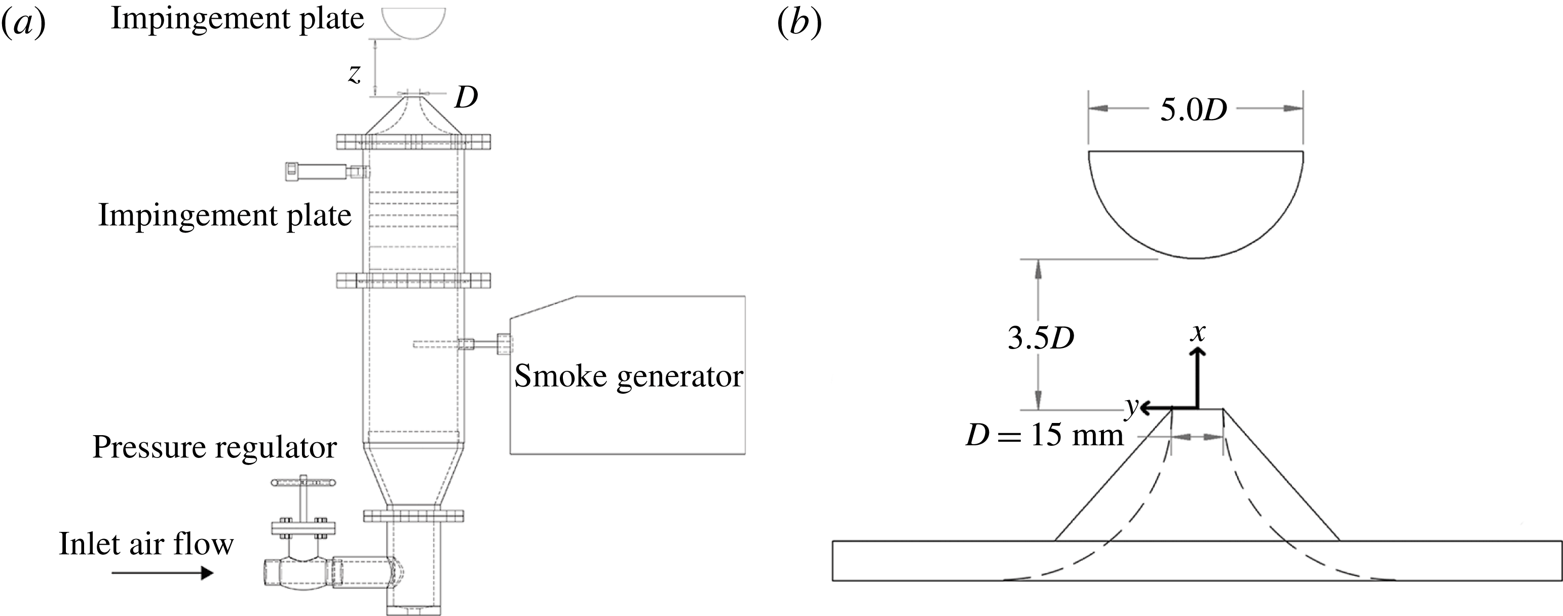
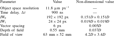
A schematic of the LTRAC gas jet facility used to acquire the PIV measurements is presented in figure 1. Full details of the experiment and acoustic measurements are available in Weightman et al. (Reference Weightman, Amili, Honnery, Soria and Edgington-Mitchell2016). The flow condition investigated is presented in table 1, where
 $M_{j}$
is the ideally expanded Mach number,
 $t$
is the lip thickness,
 $z$
is the standoff height and
 $D_{c}$
is the cylinder diameter.
(a) Schematic of the LTRAC gas jet facility. (b) Schematic of the impingement surface set-up used for the experiment.

Experimental conditions.

To produce a flow amenable to measurement with PIV, a cylinder was used in place of the more typical flat impingement surface to generate a stationary flapping instability. A cylindrical half-section with diameter
 $D_{c}=5D$
and length
 $L_{c}=7D$
was used as the impingement surface, as shown in figure 1, along with the coordinate axis.
To minimize the obscuration of key phenomena by the path-integrated nature of schlieren, some measurements were also taken using a hemispherical impingement geometry. This hemisphere had the same diameter as the cylindrical half-section. The geometry of the hemisphere causes the wall jet flow to curve away in all directions, resulting in a relatively thin flow in the light path direction. This allows for a clearer visualization of phenomena in the wall jet region. For the hemispherical impingement, flow conditions different from the cylindrical impingement case were used. A converging–diverging (CD) nozzle was operated in an underexpanded state at a nozzle pressure ratio (NPR) of 5.0. The CD nozzle had a throat diameter of 10 mm and an ideal pressure ratio of 4.0. Schlieren images were recorded from a Toepler Z-type schlieren apparatus at 500 kfps using a Shimadzu HPV-1 camera, with a resolution of
 $260\times 312~\text{px}$
and an exposure time of
 $0.5~\unicode[STIX]{x03BC}\text{s}$
.
For the velocity measurements, single exposure image pairs were acquired using a 12-bit Imperx B6640 camera with a CCD array of
 $6600\times 4400~\text{px}$
. An object space resolution of
 $11.8~\unicode[STIX]{x03BC}\text{m}~\text{px}^{-1}$
was achieved using a 200 mm Micro-Nikkor lens, with a Nikon PK-12 extension ring. The flow was seeded using a ViCount 1300 smoke generator, which produced particles of approximately 600 nm in diameter. The particles were illuminated using an expanding light sheet of approximately 1 mm thickness produced from a dual-cavity pulsed Nd:YAG laser at 532 nm, with a maximum pulse energy of 200 mJ. The pulse timing,
 $\unicode[STIX]{x0394}t$
, was 900 ns. The multigrid cross-correlation algorithm of Soria (Reference Soria1996) was used to analyse the single-exposed particle image pairs. Pixel displacements varied from
 ${<}5~\text{px}$
up to 45 px, and thus an initial window size,
 $IW_{0}$
, of
 $192\times 192~\text{px}$
and a final window size,
 $IW_{1}$
, of
 $24\times 24~\text{px}$
were selected for the PIV processing. The pertinent PIV parameters are summarized in table 2. Higher-magnification measurements were simultaneously acquired, with an object space resolution of
 $7.2~\unicode[STIX]{x03BC}\text{m}~\text{px}^{-1}$
. These measurements were focused on the impingement surface region, centred on the suspected sound production location.
Pertinent PIV parameters.

The aeroacoustic feedback process is characterized by large-scale periodic structures. To isolate these structures from the broadband turbulence, proper orthogonal decomposition (POD) (Sirovich Reference Sirovich1987; Meyer, Pedersen & Özcan Reference Meyer, Pedersen and Özcan2007; Edgington-Mitchell, Honnery & Soria Reference Edgington-Mitchell, Honnery and Soria2014a
; Edgington-Mitchell et al.
Reference Edgington-Mitchell, Oberleithner, Honnery and Soria2014b
) was applied to the PIV data. Proper orthogonal decomposition constructs a set of basis functions that optimally represent the ensemble of fluctuating velocities. The mode coefficients,
 $\boldsymbol{a}_{i}(n)$
, represent the contribution of mode
 $i$
to the total fluctuations of snapshot
 $n$
. The resultant eigenvalues are related to the specific kinetic energy of each mode. The highest energy modes are attributed to the azimuthal instability that describes the large-scale vortical structures. Due to the periodic nature of these structures, a phase average can thus be formed based on the relation between the POD mode coefficients of the dominant mode pair (Oberleithner et al.
Reference Oberleithner, Sieber, Nayeri, Paschereit, Petz, Hege, Noack and Wygnanski2011; Weightman et al.
Reference Weightman, Amili, Honnery, Soria and Edgington-Mitchell2016).
3 Identification of the sound production mechanism
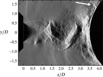
A transient shock structure in the wall jet region above the cylinder surface is highlighted in figure 2 for an NPR 3.4 flow. This structure is observed in numerous instantaneous images, with a mean position of
 $(x/D,y/D)\approx (3.8,1.4)$
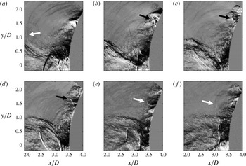
. To study the time evolution of this shocklet, an ultra-high-speed schlieren sequence of the flow is presented in figure 3, where each image is separated by
 $12~\unicode[STIX]{x03BC}\text{s}$
. To maximize the visibility of the shocklet, the hemispherical impingement surface was employed for the flow visualization. The shocklet is observed to form with the passing of a large-scale vortex along the wall (panels a and b). Shortly after its formation, the shocklet rotates to become more perpendicular to the impingement surface, while simultaneously moving slightly upstream against the wall jet flow (c and d). The upstream motion terminates with the production of an acoustic wave (e and f), shortly before the arrival of the next structure. Full-field image sequences show this acoustic wave travelling back to the nozzle lip to close the feedback loop. This is a previously unobserved phenomenon, which appears to differ from the model proposed by Henderson et al. (Reference Henderson, Bridges and Wernet2005).
The two flow conditions presented here are for different NPRs, nozzle designs and impingement geometries; however, the shocklet structure is still observed. Additionally, although not shown here, the shocklet structure has been observed across a range of NPRs (both under- and over-expanded conditions), standoff distances and impingement surfaces, including the canonical flat plate impingement geometry. While there may be other mechanisms of aeroacoustic feedback in supersonic jet impingement, the mechanism associated with the shocklet does not appear to be geometry-specific.
Schlieren visualization of the jet impinging on a cylindrical surface at an NPR of 3.4. The white arrow highlights the shocklet.

High-speed schlieren images of hemisphere impingement, separated by
 $12~\unicode[STIX]{x03BC}\text{s}$
, illustrating the formation of the shocklet structure and acoustic wave. The black arrows highlight the shocklet, with the white arrows showing the produced acoustic waves. The flow was emitted from a CD nozzle at an NPR of 5.0.

Based on these observations, two hypotheses are proposed: (1) the shocklet is the source of the impingement tone acoustic waves; (2) the time between the formation of the shocklet and the formation of the acoustic wave explains the phase lag term of the impingement feedback equation. By rearranging (1.1), we obtain
 $$\begin{eqnarray}\frac{N}{f}=\int _{0}^{h_{c}}\frac{\text{d}h}{u_{c}}+\frac{h_{s}}{U_{s}}+\unicode[STIX]{x0394}t.\end{eqnarray}$$
A time delay term has replaced the phase lag term, where
 $\unicode[STIX]{x0394}t=-p/f$
. This is the time between the shocklet inception and acoustic wave formation. Although not used further, measurement of the hemispherical schlieren data gives a time delay of
 $\unicode[STIX]{x0394}t=40~\unicode[STIX]{x03BC}\text{s}$
. With a peak tone frequency for the hemisphere impingement case of
 $12\,250~\text{Hz}$
, this delay is equivalent to a phase lag of
 $-0.49$
. Due to the thickness of the wall jet in the cylinder case, consistent measurements of the time delay were not able to be obtained. Instead, analysis of the high-resolution PIV data will provide the
 $\unicode[STIX]{x0394}t$
value for the cylinder impingement case.
The first hypothesis seems to be well supported by the ultra-high-speed schlieren (see supplementary movie 1 available at https://doi.org/10.1017/jfm.2017.37); the acoustic waves produced as a result of the shocklet structures are clearly observed propagating back to the nozzle lip. To provide support for the second hypothesis, further analysis is required. In the following sections, the various terms in the modified form of Powell’s feedback equation (3.1) are measured using acoustic measurements and high-resolution PIV for a single impingement condition. Evaluation of this equation allows for a prediction of the impingement tone frequency. This frequency can then be compared with that determined by the acoustic measurements.
4 Evaluation of the modified aeroacoustic feedback equation
To measure the values of the terms of the modified form of Powell’s impingement feedback loop equation, several experimental techniques are used. Acoustic measurements provide an estimate of the impingement tone frequency. For measurement of the acoustic wave speed, high-resolution PIV measurements are obtained. Finally, the trajectory of the large-scale vortices, convective velocity, number of concurrent cycles and time delay are found using a phase average constructed using the POD of the PIV measurements.
4.1 Impingement tone frequency
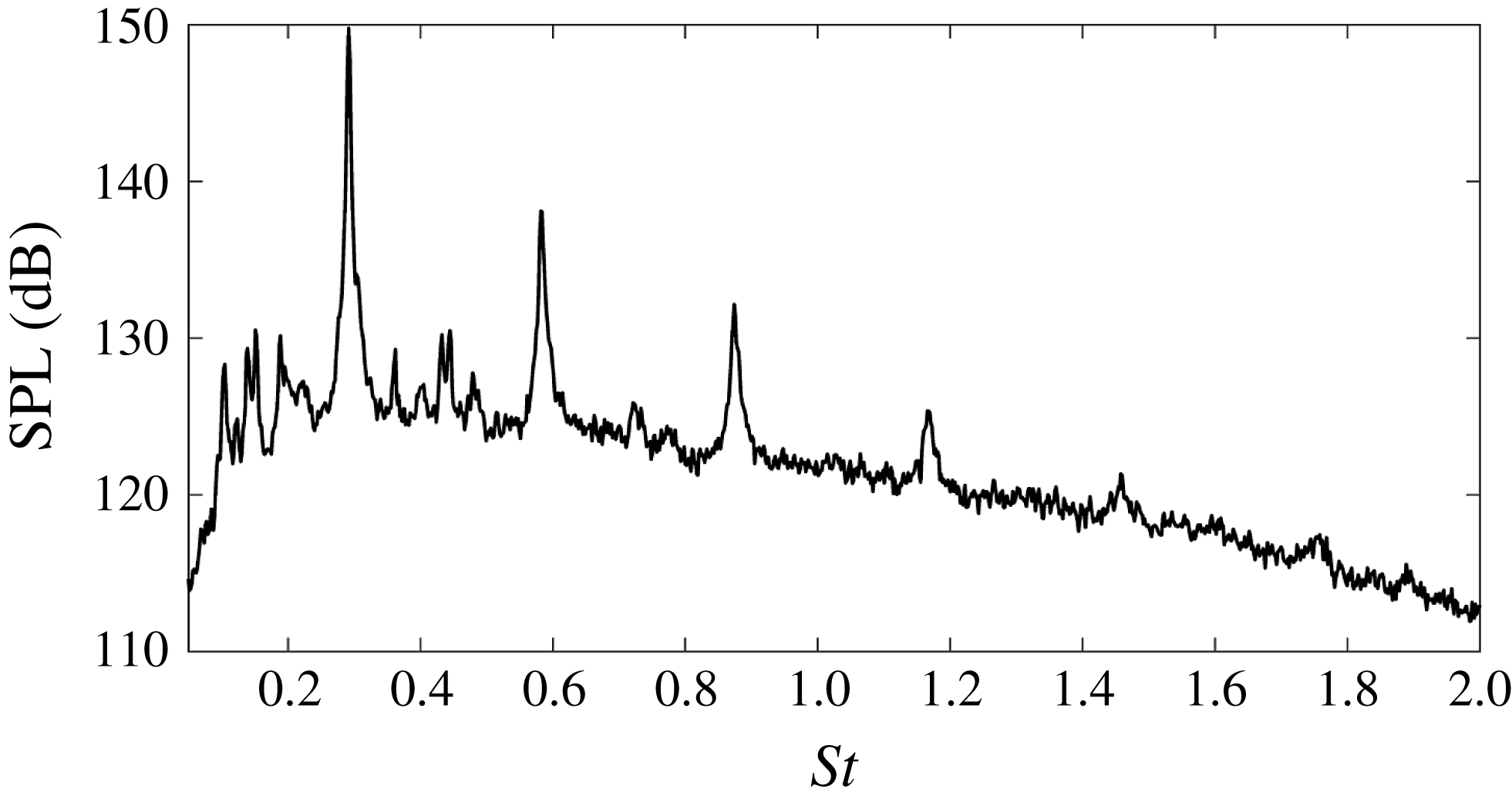
The acoustic signature generated by the jet provides information on the cyclic behaviour of the large-scale instabilities of the flow. The acoustic spectrum in figure 4 illustrates the high-intensity discrete peak associated with the impingement tone of the jet. For the cylinder impingement case studied here, this tone has a Strouhal number of
 $St=fD_{j}/U_{j}=0.29$
, where the ideally expanded jet velocity is
 $U_{j}=460.8~\text{m}~\text{s}^{-1}$
and the impingement tone frequency is
 $f=8300~\text{Hz}$
. To test the second hypothesis of § 3, the frequency predicted by the modified feedback equation will be compared with the tone frequency of the acoustic measurements.
Acoustic spectrum illustrating the tone generation of the impinging flow.

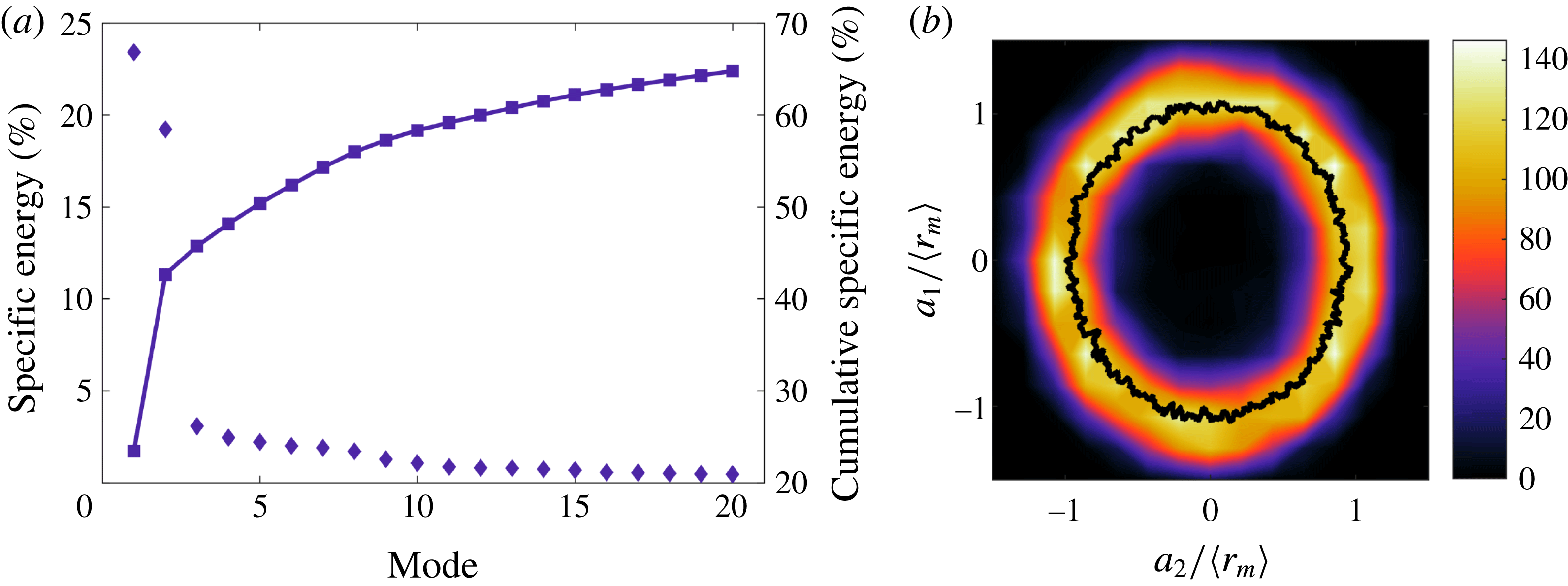
(a) Individual and cumulative energy spectra of the first 20 POD modes. (b) Joint PDF representing the phase portrait of modes 1 and 2, with a Lissajous curve overlaid. The coefficients are normalized by the mean amplitude,
 $\langle r_{m}\rangle =\overline{\sqrt{(a_{i}(t))^{2}+(a_{j}(t))^{2}}}$
.

4.2 Application of the phase average
Several of the parameters of (3.1) cannot be easily determined solely from instantaneous PIV snapshots. To measure these terms, a phase average is determined from the POD. This phase average represents a quasi-time resolved quantitative measurement of the flow. To construct the phase average, POD was undertaken on the fluctuating flow fields, producing the specific kinetic energy spectra presented in figure 5(a). The leading pair of modes contain 23.3 % and 19.0 % each of the total energy. The remaining modes each contain less than 3 % of the total energy, and are thus omitted from the subsequent analysis.
To explore the relationship between the leading modes, a phase portrait of the mode coefficients is shown in figure 5(b), with a line of mean radial position representing a Lissajous curve (Oberleithner et al.
Reference Oberleithner, Sieber, Nayeri, Paschereit, Petz, Hege, Noack and Wygnanski2011). The circular shape of this curve suggests that modes 1 and 2 are periodic and
 $90^{\circ }$
out of phase, indicating that modes 1 and 2 are a modal pair representing the azimuthal instability of the flow.
A phase average of the time independent velocity fields can be constructed from the POD mode coefficients. Intrinsic to the phase portrait of figure 5 is the phase angle,
 $\unicode[STIX]{x1D703}$
, between modes 1 and 2 for each velocity field. The phase portrait is separated into
 $5^{\circ }$
sectors, with 50 % overlap. The velocity fields in each sector are averaged, thus yielding a phase averaged measurement of the flow (see supplementary movie 2). The symmetry of the transverse fluctuation with respect to the jet centreline is indicative of an asymmetric instability mode. Given the geometry of the impingement surface, it is concluded that the mode pair represents a stationary flapping mode (Mason-Smith et al.
Reference Mason-Smith, Edgington-Mitchell, Buchmann, Honnery and Soria2015).
As the high- and low-magnification measurements were acquired simultaneously, the same phase average as determined for the lower-magnification data was applied to the higher-magnification fields. The shocklet location was estimated using the higher-magnification phase averaged velocity fields. A large velocity gradient in the direction tangential to the impingement surface was present in the wall jet throughout a portion of the phase cycle. This gradient is indicative of a shock structure, with its shape and position comparable to those observed in the high-speed schlieren of the hemisphere impingement. From the portion of the phase cycle where the gradient was most clearly defined, a position of
 $(x/D,y/D)=(3.78,1.43)$
was determined for the shocklet.
The trajectory of the vortical structures along the shear layer is represented by the line integral in the feedback equation,
 $\int _{0}^{h_{c}}\text{d}h/u_{c}$
. To track the centroids of the vortices as they travel along the shear layer, a two-dimensional swirling strength analysis (Zhou et al.
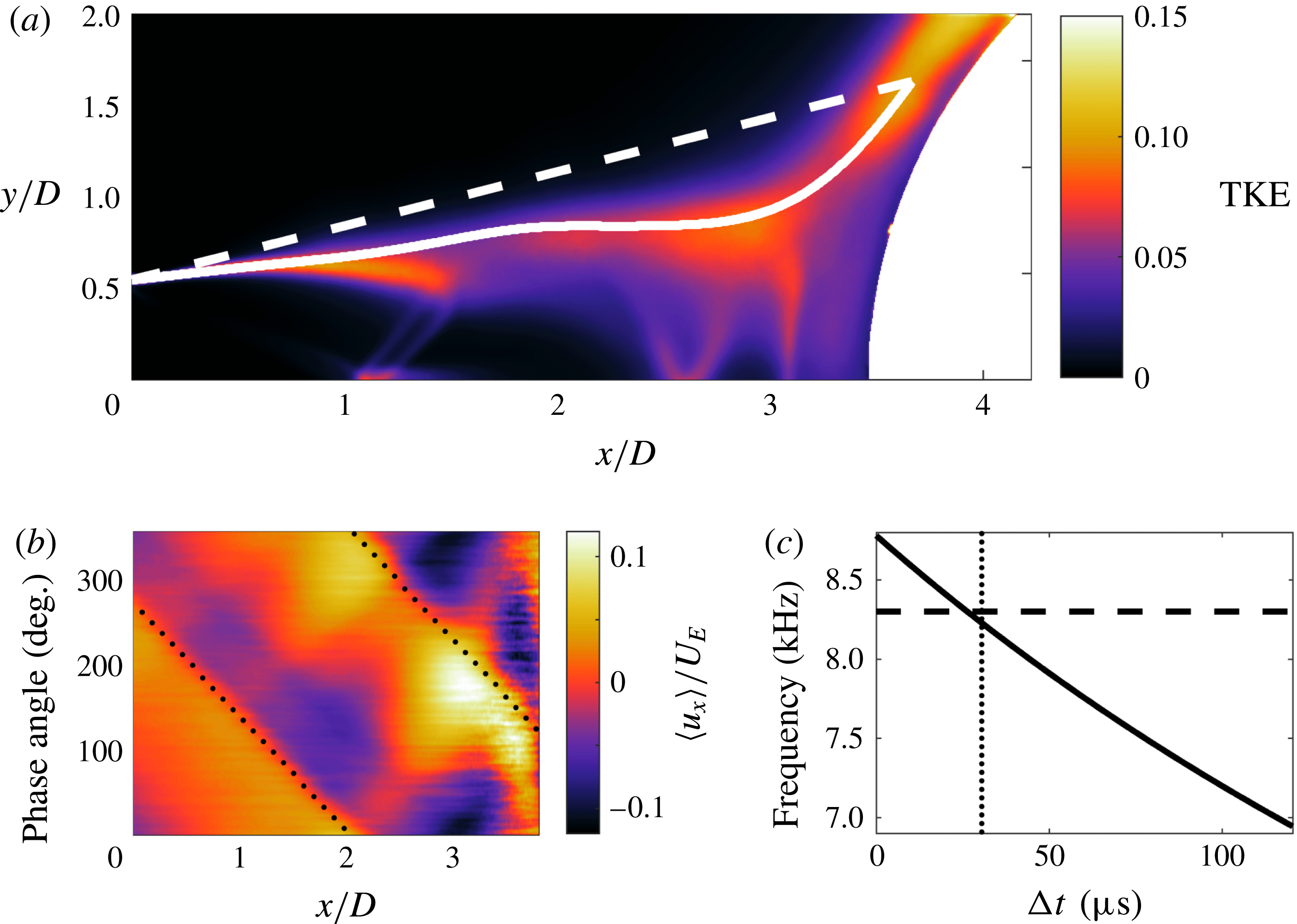
Reference Zhou, Adrian, Balachandar and Kendall1999; Adrian, Christensen & Liu Reference Adrian, Christensen and Liu2000) is applied to the phase averaged fields. The path produced closely matches the peak specific turbulent kinetic energy (TKE) along the shear layer. Thus, for regions where the centroid tracking fails, the vortex path is selected to follow the peak TKE. This path is illustrated in figure 6, ending at the measured shocklet location.
The acoustic wave propagation is modelled as a straight path of length
 $h_{s}$
, with a constant wave speed
 $U_{s}$
. The acoustic wave travels from the shocklet location back to the nozzle lip, as illustrated by figure 6(a). The acoustic wave speed is historically set to the local speed of sound (Powell Reference Powell1988; Krothapalli et al.
Reference Krothapalli, Rajkuperan, Alvi and Lourenco1999). However, this does not account for the entrainment velocity. In the present work, detailed measurements of the velocity field allow for a more precise estimate of the acoustic wave speed in the Eulerian frame. The entrainment velocity in the present case has a mean axial component of approximately
 $9~\text{m}~\text{s}^{-1}$
. Setting the local speed of sound to
 $340~\text{m}~\text{s}^{-1}$
, this results in an estimated acoustic wave speed of
 $331~\text{m}~\text{s}^{-1}$
in a fixed reference frame.
(a) Illustration of the path of the feedback loop: ——, path of the large-scale vortical structures; - - - -, path of the acoustic waves. (b) Evolution of an axial vector line at
 $y/D=1.45$
of the phase averaged axial fluctuations through the phase cycle:
 $\cdots \cdots$
, trace of an acoustic wave. (c) Predicted acoustic frequency for varying time delay:
 $\cdots \cdots$
, value obtained in § 5; - - - -, measured frequency value.

The convective velocity of the large-scale vortices can be extracted from the trajectory of the peak transverse velocity in the phase averaged data. Recognizing that one phase cycle is equal to
 $120.5~\unicode[STIX]{x03BC}\text{s}$
, the convective velocity ranges from
 $0.42U_{j}$
to
 $0.52U_{j}$
, with a mean value of
 $0.48U_{j}$
. The peak detection used is inconsistent outside of
 $0.75<x/D<2.6$
, and so the end point convective values are substituted for the corresponding portions of the line integral.
The number of concurrent cycles can also be determined from the phase averaged PIV data. Four new vortices are generated at the nozzle lip in the time it takes for one feedback cycle to complete; thus,
 $N=4$
.
Without clear high-speed schlieren visualizations of the shocklet for the cylindrical impingement, the time delay value must be determined from the PIV. Acoustic waves in the entrainment region are present in the phase averaged data. These waves are observed to propagate upstream towards the nozzle through the phase cycle. The point in the phase cycle when the acoustic waves are produced can be determined by tracing the acoustic waves back to the impingement surface. This method can be seen in figure 6(b), where the phase angle of the sound production is found when the dotted line reaches
 $x/D=3.8$
. This gives a value of
 $\unicode[STIX]{x1D703}=122.5^{\circ }$
.
To determine the time delay, the point in the phase cycle when the shocklet forms is required. From the schlieren of the hemisphere impingement, the shocklet forms with the passing of a large-scale vortex. To determine when this occurs, the vortex can be tracked from the nozzle lip to the measured shocklet location using the convective velocity along the vortex path. The point in the phase cycle when the acoustic wave reaches the nozzle lip is at
 $\unicode[STIX]{x1D703}=262.5^{\circ }$
, as determined from figure 6(b) when the dotted line reaches
 $x/D=0$
. Adding to this the vortex convection time, and accounting for complete phase cycles, the arrival point of the vortex at the shocklet location is calculated as
 $\unicode[STIX]{x1D703}=34.5^{\circ }$
.
The time delay due to the existence of the shocklet is thus given by the phase difference between the above two events. This can easily be found as the shocklet formation time and acoustic production are assumed to occur within one phase cycle. Again, since one phase cycle is equal to
 $120.5~\unicode[STIX]{x03BC}\text{s}$
, a time delay value of
 $\unicode[STIX]{x0394}t=29.4~\unicode[STIX]{x03BC}\text{s}$
is obtained for the cylindrical impingement case. From the high-speed schlieren, this process is observed to be unsteady. As this time delay was calculated from a phase average, the variation of the value cannot be determined here.
5 Results of the modified feedback equation
In the preceding sections, all terms in (3.1) have been directly measured. Using the values obtained from the PIV data, (3.1) predicts a frequency of
 $f=8230~\text{Hz}$
. This closely matches the actual impingement frequency, with a difference of 0.8 % of the measured tone. This agreement offers strong support for the hypothesis that the time delay caused by the shocklet explains the phase lag term of Powell’s feedback equation. For comparison, evaluation of (3.1) with a time delay of
 $\unicode[STIX]{x0394}t=0$
results in a predicted frequency of
 $f=8750~\text{Hz}$
, 5.4 % higher than the measured tone.
To provide further support to the second hypothesis, the sensitivity of the predicted frequency to time delay is determined. Given that
 $p/f=-\unicode[STIX]{x0394}t$
, the time delay term must be between 0 and
 $120.5~\unicode[STIX]{x03BC}\text{s}$
, which also implies
 $-1\leqslant p\leqslant 0$
. The variation of the predicted frequency in response to changing time delay is presented in figure 6(c). The predicted frequency varies significantly over the range of possible time delays (
 $f=6920{-}8750~\text{Hz}$
). To correct for the change in predicted frequency for a zero time delay, the mean convective velocity would need to decrease by approximately
 $0.05U_{j}$
to
 $U_{c}=0.43$
. This value is only slightly above the lowest convective velocity measured here, and significantly lower than that reported in the literature. It is improbable that the actual convective velocity is this low, and thus the inclusion of the time delay due to the shocklet is necessary to obtain a good agreement between the predicted and measured frequencies.
6 Conclusions
From ultra-high-speed schlieren, a periodic transient shock structure is identified in the wall jet region of underexpanded impinging flows. It is hypothesized that the shocklet is the sound source of the impingement tones and that the lifetime of the shocklet explains the phase lag term in the impingement feedback equation (Powell Reference Powell1988). To test this hypothesis, a modified feedback equation is formed using an equivalent time delay. The values measured from high-resolution PIV allow for a prediction of the impingement tone frequency, which is compared with the tone measured by a microphone measurement.
Close agreement between the predicted and measured frequencies supports the hypothesis that the shocklet is an integral component of the sound production mechanism and the aeroacoustic feedback process, explaining the presence of the phase lag term described by Powell (Reference Powell1988). Additionally, if the time delay were zero, the large change in convective velocity required for the predicted and measured frequencies to match would be implausible. This further supports the hypothesis that the shocklet explains the phase lag term of the aeroacoustic feedback process.
Acknowledgements
The authors would like to thank N. Mason-Smith for supplying the high-resolution schlieren image presented in figure 2. This research was supported under the Australian Research Council’s Discovery Projects funding scheme. This research was undertaken with the assistance of resources provided at the NCI National Facility systems at the Australian National University through the National Computational Merit Allocation Scheme supported by the Australian Government.
Supplementary movies
Supplementary movies are available at https://doi.org/10.1017/jfm.2017.37.