INTRODUCTION
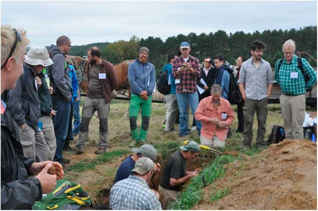
In September 2016, the annual meeting of the International Union for Quaternary Research’s (INQUA) Loess and Pedostratigraphy Focus Group met in western Wisconsin, USA. This focus group is part of INQUA’s Commission on Stratigraphy and Chronology (https://www.inqua.org/commissions/saccom). Meetings of this group have traditionally been referred to as LoessFests. The 2016 LoessFest focused on “thin” loess deposits and loess transportation surfaces. Held in Eau Claire, Wisconsin, from September 22 to 25, this LoessFest included 75 registered participants from 10 countries. Almost half of the participants were from outside the United States, and 18 of the participants were students. In all, 29 oral papers and 14 posters were presented during the first two days. Kathleen Goff (University of Iowa) won the award for the best student poster, and Rastko Marković (University of Novi Sad, Serbia) won the award for the best student oral paper. The last two days of the conference involved field trips to sites in western Wisconsin. The trips included 13 stops, most of which were exposures or backhoe pits in loess or related sediments (Fig. 1).
(color online) Participants taking turns examining thin loess in a soil pit at one of the several field trip stops at the 2016 LoessFest in western Wisconsin, USA. Photo by. R. Schaetzl.

After the meeting, the conference organizers were approached by Quaternary Research and Aeolian Research about developing special issues for these journals, dedicated to topics focusing on loess. This review represents the introduction to the special issue for Quaternary Research. The goals of this introduction are to (1) provide brief summaries of some of the current approaches/strategies used to study loess deposits and, in so doing, (2) highlight some of the ongoing work on loess in various regions of the world. Numerous examples from, and reviews of, some of the world’s major loess deposits are discussed first to provide context. We hope that these summaries, written by a selection of the world’s most prominent loess researchers, will not only highlight the fascinating world of loess research, but also draw attention to loess-related questions, approaches, and methods that may form the basis of future research.
(MOST OF) THE WORLD’S MAJOR LOESS DEPOSITS
Loess in China
By Shiling Yang
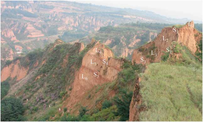
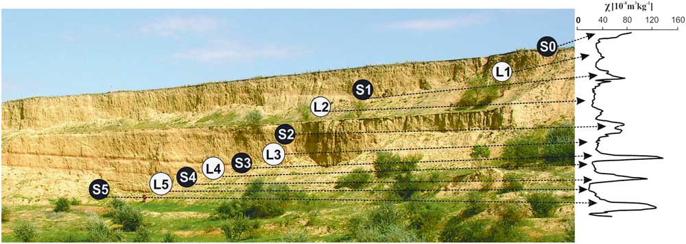
Loess deposits in China are widely distributed across the Chinese Loess Plateau (Fig. 2), where they attain thicknesses ranging from several tens of meters to >300 m, across an area of ~273,000 km2 (Liu, Reference Liu1985). The thickest and most complete loess sequences occur mainly in the central and southern parts of the plateau, where they range from 130 to 200 m thick and consist of as many as 34 loess-paleosol couplets (Fig. 3; Yang and Ding, Reference Yang and Ding2010). As per standard nomenclature, loess horizons are labeled L i and the intercalated paleosols S i . Several loess and paleosol units are usually used as stratigraphic markers across the Chinese Loess Plateau, including thick and coarse-grained loess units L9, L15, L24, L27, and L32, and strongly developed paleosols S5 and S26 (Ding et al., Reference Ding, Rutter and Liu1993, Reference Ding, Derbyshire, Yang, Yu, Xiong and Liu2002a). The alternation of loess and paleosols reflects large-scale oscillations between glacial conditions, when loess accumulates, and interglacial conditions, when loess deposition wanes and soils form.
Map of loess deposits (yellow) on the Chinese Loess Plateau. Arrows indicate the direction of the East Asian winter and summer monsoonal winds. Inset shows the location of the Chinese Loess Plateau in Euroasia. After Yang et al. (Reference Yang, Ding, Li, Wang, Jiang and Huang2015). (For interpretation of the references to color in this figure legend, the reader is referred to the web version of this article.)

(color online) Photograph of the eolian deposits at Luochuan (Fig. 1), in the central Chinese Loess Plateau, with loess (L)–soil (S) couplets for the L1–L6 portion indicated. For details on stratigraphic nomenclature of Chinese loess, see Rutter et al. (Reference Rutter, Ding, Evans and Liu1991) and Ding et al. (Reference Ding, Rutter and Liu1993). Photo by Shiling Yang.

The modern climate of the Chinese Loess Plateau is characterized by the seasonal alternation of summer and winter monsoons. During winter, the northwesterly monsoonal winds driven by the Siberian High dominate the Chinese Loess Plateau and lead to cold and dry weather, whereas in summer, the southeasterly monsoonal winds bring heat and moisture from the low-latitude oceans, leading to warm and humid weather. Meteorologic data indicate that ~60–80% of annual precipitation is concentrated in the summer season (Yang et al., Reference Yang, Ding, Wang, Tang and Gu2012, Reference Yang, Ding, Li, Wang, Jiang and Huang2015).
Loess material in northern China is likely to have first formed through glacial abrasion and erosion by other geomorphic processes in mountainous areas (Sun, Reference Sun2002b; Smalley et al., Reference Smalley, O’Hara-Dhand and Kwong2014), then was transported by fluvial and eolian processes into deserts, which act as silt and clay storage regions, rather than places where particles are formed. The eolian dust that constitutes the loess is mainly transported from these deserts by the winter monsoon, whereas the postdepositional alteration of dust deposits is closely related to the precipitation provided by the summer monsoon (Liu, Reference Liu1985; Liu and Ding, Reference Liu and Ding1998). Therefore, Chinese loess deposits provide a unique opportunity to investigate the evolution of the East Asian monsoon over the past 2.8 Ma (Yang and Ding, Reference Yang and Ding2010) and the complex interactions of Earth surface-climate systems (Sun, Reference Sun2002a; Smalley et al., Reference Smalley, O’Hara-Dhand and Kwong2014).
Studies of Chinese loess have shown that various proxy records in the loess column can reveal abundant information on regional climatic and environmental changes. The most common paleoenvironmental proxies used here are magnetic susceptibility (Kukla et al., Reference Kukla, Heller, Liu, Xu, Liu and An1988; An et al., Reference An, Kukla, Porter and Xiao1991a), grain size (An et al., Reference An, Kukla, Porter and Xiao1991b; Ding et al., Reference Ding, Yu, Rutter and Liu1994), chemical weathering indexes (Gallet et al., Reference Gallet, Jahn and Torii1996; Chen et al., Reference Chen, An and Head1999; Yang et al., Reference Yang, Ding and Ding2006), isotopic ratios (Liu et al., Reference Liu, Yang, Sun and Wang2011; Yang et al., Reference Yang, Ding, Wang, Tang and Gu2012), soil micromorphology (Bronger and Heinkele, Reference Bronger and Heinkele1989; Rutter and Ding, Reference Rutter and Ding1993), biomarkers (Peterse et al., Reference Peterse, Martínez-García, Zhou, Beets, Prins, Zheng and Eglinton2014; Li et al., Reference Li, Yang, Wang, Hu, Cui, Huang and Jiang2016b; Thomas et al., Reference Thomas, Clemens, Sun, Prell, Huang, Gao, Loomis, Chen and Liu2016), and pollen, snail, and opal phytolith assemblages (Lu et al., Reference Lu, Wu, Liu, Jiang and Liu2007; Rousseau et al., Reference Rousseau, Wu, Pei and Li2009; Jiang et al., Reference Jiang, Cheng, Yang and Yang2013, Reference Jiang, Yang and Cheng2014). In the last few decades, many studies have focused on the evolution of the East Asian monsoon and regional tectonic uplift (e.g., Liu and Ding, Reference Liu and Ding1998 and references therein; Maher, Reference Maher2016 and references therein), using mainly proxy data from loess deposits. The East Asian monsoon varies over tectonic to millennial time scales but is mostly driven by Northern Hemisphere glacial cyclicity (Ding et al., Reference Ding, Derbyshire, Yang, Yu, Xiong and Liu2002a, Reference Ding, Derbyshire, Yang, Sun and Liu2005; Yang and Ding, Reference Yang and Ding2014). On tectonic (i.e., the longest) time scales, since the mid-Pliocene there appears to have been a stepwise weakening of the East Asian summer monsoon at 2.6, 1.2, 0.7, and 0.2 Ma (Ding et al., Reference Ding, Derbyshire, Yang, Sun and Liu2005). On orbital time scales, the East Asian summer (winter) monsoon weakened (strengthened) during glacial periods, and vice versa during interglacial periods, leading to a 200 to 300 km advance-retreat of the desert boundary (Yang and Ding, Reference Yang and Ding2008) and its associated vegetation changes (Jiang et al., Reference Jiang, Cheng, Yang and Yang2013, Reference Jiang, Yang and Cheng2014; Yang et al., Reference Yang, Ding, Li, Wang, Jiang and Huang2015) in northern China. As for the millennial-scale climate variability, high-resolution grain-size data from the Chinese loess deposits show that millennial-scale climatic events are superimposed onto a prominent long-term cooling trend, during both the last and penultimate glaciations (Yang and Ding, Reference Yang and Ding2014). However, millennial-scale ecological reconstructions of the Chinese Loess Plateau remain to be investigated.
Although the foundational work on Chinese loess, such as the major stratigraphic, chronological, sedimentologic, and paleoclimatic frameworks, has already been established (Liu and Ding, Reference Liu and Ding1998; Ding et al., Reference Ding, Derbyshire, Yang, Yu, Xiong and Liu2002a), there remains a great deal of work to be done. First, accurate quantitative reconstructions of temperature and precipitation are needed to improve existing ones, and there is a need to develop new methods and approaches for quantitative paleoenvironmental and paleoclimatic reconstructions. These reconstructions are challenging. Second, it is crucial to investigate whether the exceptionally coarse-grained units (e.g., L9, L15, and L33) in the Chinese loess deposits are the products of enhanced erosion produced by tectonic uplift of mountains in Asia (Sun and Liu, Reference Sun and Liu2000; Wu and Wu, Reference Wu and Wu2011) or of extreme regional climatic events (Ding et al., Reference Ding, Derbyshire, Yang, Yu, Xiong and Liu2002a). Third, the provenance of Chinese loess remains a highly debated topic (Sun, Reference Sun2002a; Pullen et al., Reference Pullen, Kapp, McCallister, Chang, Gehrels, Garzione, Heermance and Ding2011; Che and Li, Reference Che and Li2013; Stevens et al., Reference Stevens, Carter, Watson, Vermeesch, Andò, Bird, Lu, Garzanti, Cottam and Sevastjanova2013b; Nie et al., Reference Nie, Stevens, Rittner, Stockli, Garzanti, Limonta and Bird2015), mainly because of varying interpretations of geochemical proxies used for determining the main source areas. The controversy centers on whether the loess deposits come from the deserts to the west or to the north of the Loess Plateau. A possible solution in this regard would be to combine geochemical data with the data on the spatiotemporal changes in sedimentologic characteristics of Chinese loess to gain a better insight into past loess source areas (Liu, Reference Liu1966; Yang and Ding, Reference Yang and Ding2008). Finally, modeling studies of dust production, transport, and deposition are required to fully understand the processes responsible for the formation of the loess deposits across the Chinese Loess Plateau.
Loess in central Asia
By Kathryn E. Fitzsimmons, Charlotte Prud’homme, and Aditi K. Dave
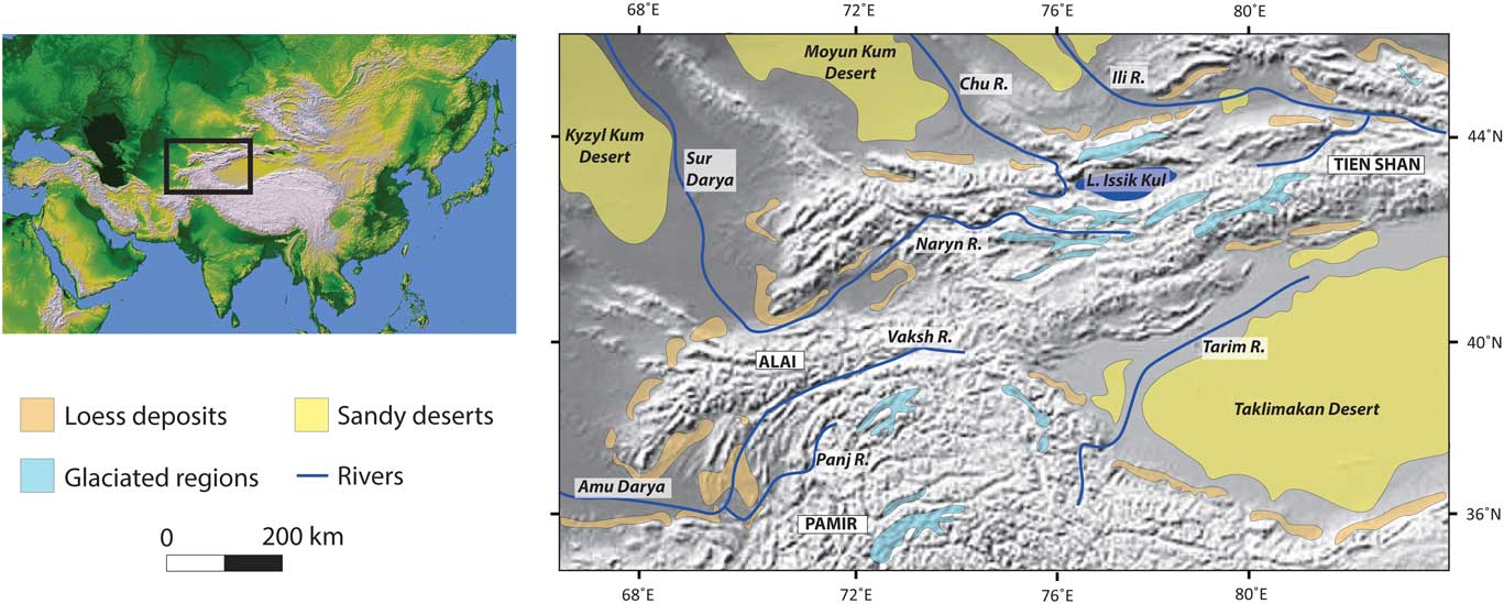
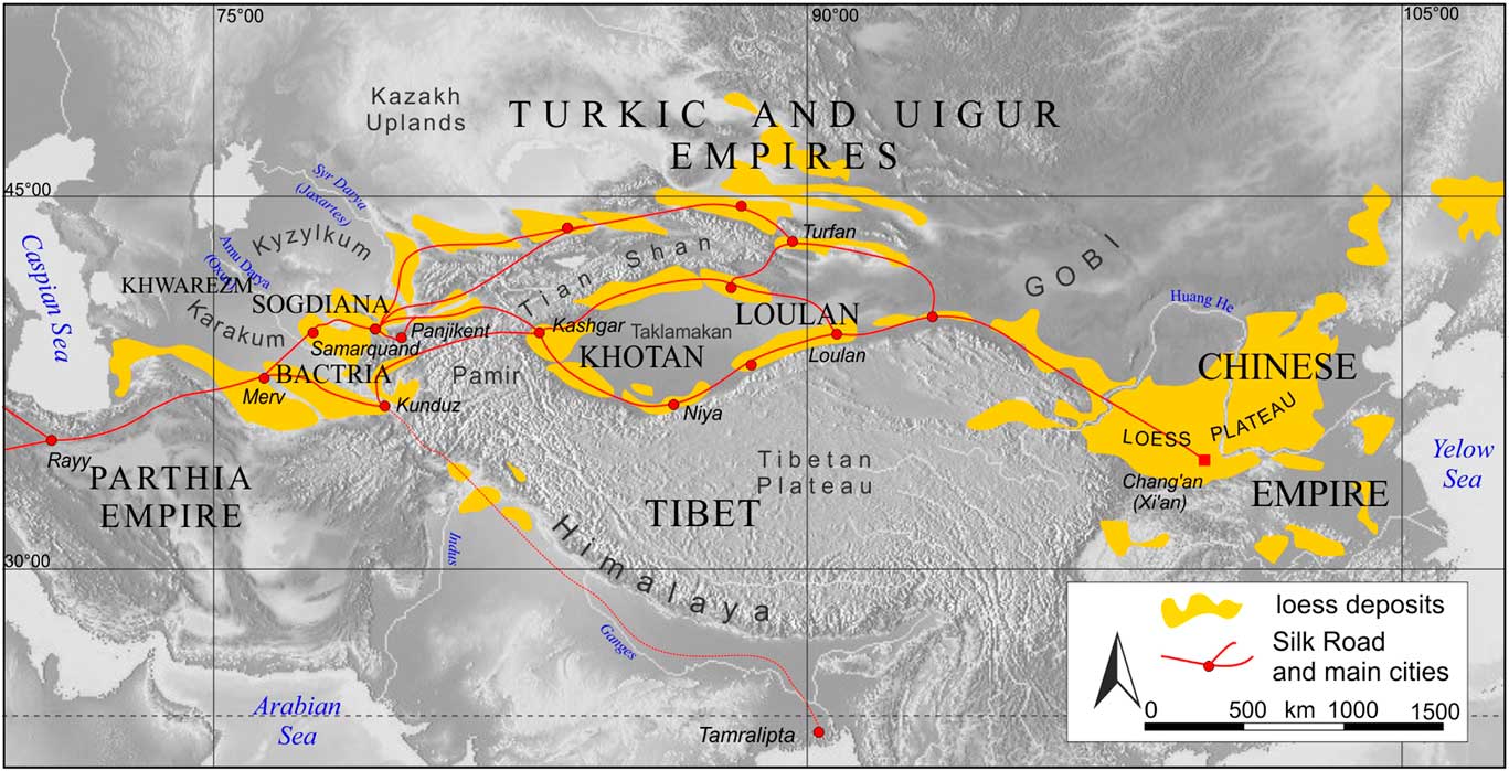
Central Asia is characterized by comparatively patchy piedmont deposits of loess of varying thickness, in contrast to other regions of the world. The widespread riverine loess steppe of the Russian Plain has a distinctly different character and is therefore not included in our definition. We define the central Asian piedmont deposits as extending from the foothills of the north Iranian Alborz/Elbruz Mountains at their westernmost extent (Kehl et al., Reference Kehl, Sahvati, Ahmadi, Frechen and Skowronek2005; Vlaminck et al., Reference Vlaminck, Kehl, Lauer, Shahriari, Sharifi, Eckmeier, Lehndorff, Khormali and Frechen2016), eastward to the Pamir and Alai ranges (Dodonov and Baiguzina, Reference Dodonov and Baiguzina1995; Dodonov, Reference Dodonov2002), the Tien Shan (Youn et al., Reference Youn, Seong, Choi, Abdrakhmatov and Ormukov2014; Fitzsimmons et al., Reference Fitzsimmons, Sprafke, Zielhofer, Günter, Deom, Sala and Iovita2016, Reference Fitzsimmons, Iovita, Sprafke, Glantz, Talamo, Horton, Beeton, Alipova, Bekseitov, Ospanov, Deom, Sala and Taimagambetov2017), and north along the Altai (Zykina and Zykin, Reference Zykina and Zykin2012; Zykin and Zykina, Reference Zykin and Zykina2015) and Mongolian Hangay (Lehmkuhl and Haselein, Reference Lehmkuhl and Haselein2000; Lehmkuhl et al., Reference Lehmkuhl, Hilgers, Fries, Hülle, Schlütz, Shumilovskikh, Felauer and Protze2011) mountain margins. The loess deposits around the Tarim basin rim may also be considered part of the central Asian piedmont loess because of their geographic similarities (Zheng et al., Reference Zheng, Chen and Cao2002, Reference Zheng, Powell, Butcher and Cao2003). Figure 4 shows the general distribution of loess deposits across the core of this region (after Dodonov, Reference Dodonov1991).
(color online) Loess distribution along the core central Asian piedmonts in the rain shadow of the Asian high mountains, showing geographic associations of loess deposits to glaciated regions, major rivers and deserts, as well as key regions and localities. After Dodonov (Reference Dodonov1991).

The active uplift of the central Asian high mountains (Campbell et al., Reference Campbell, Walker, Abdrakhmatov, Jackson, Elliott, Mackenzie, Middleton and Schwenninger2015; Grützner et al., Reference Grützner, Carson, Walker, Rhodes, Mukambayev, Mackenzie, Elliott, Campbell and Abdrakhmatov2017) results in steep, rugged terrain, effectively preventing wide-scale accumulation and development of loess plateaus. This central Asian piedmont, set in the rain shadow of the Asian high mountains, generally experiences a semiarid continental climate. Climatic parameters vary more specifically with altitude, latitude, orographic effects, and the relative influences of the major Northern Hemisphere climate subsystems. The dominant climatic influences are the midlatitude westerlies, northerly polar fronts, the Siberian high pressure system, and East Asian and Indian monsoon systems (Dettman et al., Reference Dettman, Kohn, Quade, Ryerson, Ojha and Hamidullah2001; Vandenberghe et al., Reference Vandenberghe, Renssen, van Huissteden, Nugteren, Konert, Lu, Dodonov and Buylaert2006; Machalett et al., Reference Machalett, Oches, Frechen, Zöller, Hambach, Mavlyanova, Markovic and Endlicher2008).
The thickest sections of central Asian piedmont loess extend beyond the Brunhes-Matuyama paleomagnetic reversal (Dodonov and Baiguzina, Reference Dodonov and Baiguzina1995; Shackleton et al., Reference Shackleton, An, Dodonov, Gavin, Kukla, Ranov and Zhou1995; Ding et al., Reference Ding, Ranov, Yang, Finaev, Han and Wang2002b; Wang et al., Reference Wang, Wei, Taheri, Khormali, Danukalova and Chen2016). As such, they represent long sediment archives that may provide a wealth of potential paleoclimatic information (Vandenberghe et al., Reference Vandenberghe, Renssen, van Huissteden, Nugteren, Konert, Lu, Dodonov and Buylaert2006; Yang and Ding, Reference Yang and Ding2006; Machalett et al., Reference Machalett, Oches, Frechen, Zöller, Hambach, Mavlyanova, Markovic and Endlicher2008). Despite the location of these deposits in a sensitive transitional climatic zone, however, relatively little is known about the past environmental history of this region, in part because of political history and logistical challenges.
Loess formation in central Asia was generally assumed to be genetically linked to sediments generated by glaciers and rivers in the mountains, which flow into the desert basins to the north and from which fine-grained dust is transported back onto the piedmonts (Aubekerov, Reference Aubekerov1993; Smalley, Reference Smalley1995; Smalley et al., Reference Smalley, Mavlyanova, Rakhmatullaev, Shermatov, Machalett, O’Hara Dhand and Jefferson2006, Reference Smalley, O’Hara-Dhand, Wint, Machalett, Jary and Jefferson2009). Because numerical chronologies for loess and glaciation in this region were lacking until recently, scholars assumed that periods of peak loess flux corresponded to cold glacial phases, and pedogenesis corresponded with interglacial periods (Ding et al., Reference Ding, Ranov, Yang, Finaev, Han and Wang2002; Vandenberghe et al., Reference Vandenberghe, Renssen, van Huissteden, Nugteren, Konert, Lu, Dodonov and Buylaert2006; Machalett et al., Reference Machalett, Oches, Frechen, Zöller, Hambach, Mavlyanova, Markovic and Endlicher2008). This assumption implied an overwhelming and continuous influence of the North Atlantic westerlies on the region and has been recently challenged. Direct dating of glacial moraines showed that some central Asian glaciers expanded during warmer, wetter phases such as Marine Oxygen Isotope Stage (MIS) 3 (Koppes et al., Reference Koppes, Gillespie, Burke, Thompson and Stone2008), and that the timing of glacial expansion varied across the Asian high mountains (Owen and Dortch, Reference Owen and Dortch2014). Subsequent dating of piedmont loess deposits also showed variable timing and rates of accumulation (Song et al., Reference Song, Lai, Li, Chen and Wang2015; Fitzsimmons et al., Reference Fitzsimmons, Sprafke, Zielhofer, Günter, Deom, Sala and Iovita2016, Reference Fitzsimmons, Iovita, Sprafke, Glantz, Talamo, Horton, Beeton, Alipova, Bekseitov, Ospanov, Deom, Sala and Taimagambetov2017; Li et al., Reference Li, Song, Chen, Li, Mamadjanov and Aminov2016a). Proxy data relating to paleoenvironmental conditions relating to temperature, precipitation, influence of specific climate subsystems, and geomorphic stability are so far limited. Data are limited either through lack of direct chronological information (Vandenberghe et al., Reference Vandenberghe, Renssen, van Huissteden, Nugteren, Konert, Lu, Dodonov and Buylaert2006; Yang and Ding, Reference Yang and Ding2006; Yang et al., Reference Yang, Ding and Ding2006; Machalett et al., Reference Machalett, Oches, Frechen, Zöller, Hambach, Mavlyanova, Markovic and Endlicher2008) or because of insufficient chronological depth of the available paleoenvironmental proxies (Dodonov et al., Reference Dodonov, Sadchikova, Sedov, Simakova and Zhou2006; Feng et al., Reference Feng, Ran, Yang, Zhai, Wang, Zhang and Huang2011; Fitzsimmons et al., Reference Fitzsimmons, Sprafke, Zielhofer, Günter, Deom, Sala and Iovita2016; Ghafarpour et al., Reference Ghafarpour, Khormali, Balsam, Karimi and Ayoubi2016).
The current state of knowledge for the region indicates variable influence of the different climate subsystems over the region and through time. One recent hypothesis suggests that loess accumulation in the central Asian piedmont peaks under two scenarios (Fitzsimmons et al., Reference Fitzsimmons, Sprafke, Zielhofer, Günter, Deom, Sala and Iovita2016). Under the first scenario, loess flux increases because of the increased sediment availability facilitated by glacial expansion—resulting from increased mountain precipitation attributable to northward monsoon migration—combined with compression of the midlatitude westerlies against the glaciated mountains and increasing wind strength (e.g., during MIS 3). Under the second scenario, loess deposition increases under cold, dry glacial conditions with reduced but sustained ice volume and persistent westerly winds (e.g., the last glacial maximum). So far, the climate mechanisms driving this hypothesis remain unidentified.
Elucidating climatic patterns from loess across central Asia through time will require targeted investigations covering the entire piedmont and applying methods that provide meaningful information addressing gaps in our understanding. Robust, long-term chronological frameworks—for example, exploiting new luminescence dating protocols (e.g., Pickering et al., Reference Pickering, Jacobs, Herries, Karkanas, Bar-Matthews, Woodhead, Kappen, Fisher and Marean2013; Ankjærgaard et al., Reference Ankjærgaard, Guralinik, Buylaert, Reimann, Yi and Wallinga2016; Liu et al., Reference Liu, Murray, Buylaert, Jain, Chen and Lu2016; Wintle and Adamiec, Reference Wintle and Adamiec2017)—are required to place proxy paleoclimatic data in context. Meaningful proxies that quantify climatic parameters, such as temperature, precipitation, and seasonality (e.g., Peterse et al., Reference Peterse, Martínez-García, Zhou, Beets, Prins, Zheng and Eglinton2014; Prud’Homme et al., Reference Prud’Homme, Antoine, Moine, Turpin, Huguenard, Robert and Degeai2015), are important future tools for clarifying the influence of climatic subsystems on the region through time. These should always be combined with classical measures of physical characteristics collected at high resolution (e.g., Vandenberghe et al., Reference Vandenberghe, Renssen, van Huissteden, Nugteren, Konert, Lu, Dodonov and Buylaert2006; Zeeden et al., Reference Zeeden, Hambach, Veres, Fitzsimmons, Obreht, Bösken and Lehmkuhl2016a) and measures of loess sediment provenance facilitating wind regime reconstruction (e.g., Újvári et al., Reference Újvári, Varga, Ramos, Kovács, Németh and Stevens2012; Stevens et al., Reference Stevens, Adamiec, Bird and Lu2013a, Reference Stevens, Carter, Watson, Vermeesch, Andò, Bird, Lu, Garzanti, Cottam and Sevastjanova2013b; Li et al., Reference Li, Song, Chen, Li, Mamadjanov and Aminov2016a). These approaches herald a new direction for loess research in this poorly understood region that may be the key to global paleoclimate reconstruction.
Loess in Europe
By Frank Lehmkuhl, Dominik Faust, Ulrich Hambach, Slobodan B. Marković, Igor Obreht, Denis-Didier Rousseau, and Jef Vandenberghe
Loess is one of the most extensively distributed terrestrial Pleistocene deposits in Europe. The thickness of loess varies between a few decimeters to several tens of meters, depending on its proximity to the source area and the geomorphological setting. Because of its wide distribution, loess is often studied in thick stratigraphic sequences interbedded with paleosols (loess-paleosol sequences [LPSs]). LPSs are the most intensively and extensively studied terrestrial archives for the reconstruction of environmental and climatic changes of glaciations in Europe, since the 1950s. This work has continued onward in the context of the International Union for Quaternary Research’s Loess Commission (e.g., Gullentops, Reference Gullentops1954; Fink, Reference Fink1956; Pécsi, Reference Pécsi1966; Fink and Kukla, Reference Fink and Kukla1977; Kukla, Reference Kukla1977; Lautridou, Reference Lautridou1981). Often these studies focused on stratigraphic subdivisions and correlations (e.g., Paepe, Reference Paepe1966) and were based on field data from sites that have given their name to classical lithostratigraphic horizons (e.g., Rocourt, Kesselt).
Maps of loess in Europe were first presented by Grahmann (Reference Grahmann1932) and later by Fink et al. (Reference Fink, Haase and Ruske1977); the most recent compilations were published by Haase et al. (Reference Haase, Fink, Haase, Ruske, Pécsi, Richter, Altermann and Jäger2007) and Bertan et al. (2016). In Europe, loess is distributed across several main regions (Fig. 5): (1) the northern European loess belt, south of the Weichselian (Marine Oxygen Isotope Stage [MIS] 2) ice margin in the north, extending to the uplands in the south (e.g., Ardennes, Rhenish shield, Harz Mountains, Ore Mountains, Karkonosze Mountains, and northern Carpathians [Tatra]); (2) eastern Europe (east of the Carpathians), including eastern Romania, Moldova, southeastern Poland, Ukraine, western Kazakhstan, and Russia; (3) the Upper Rhine Valley and the basins of the mountainous areas in central and southwestern Germany, including Bohemia and Moravia in Česká; and (4) along the Danube River, from Bavaria toward Austria, Hungary, Slovakia, Croatia, Serbia, Romania, and northern Bulgaria. Small patches of loess also occur in southern and Mediterranean parts of Europe, mainly in Spain and along the Rhone River in southern France. Minor, although paleoclimatically important loess deposits, also occur in the Po plain of Italy and along the northern Adriatic coast (Cremaschi et al., Reference Cremaschi, Zerboni, Nicosia, Negrino, Rodnight and Spötl2015; Wacha et al., Reference Wacha, Rolf, Hambach, Frechen, Galović and Duchoslav2017).
(color online) Loess distribution map (Haase et al., Reference Haase, Fink, Haase, Ruske, Pécsi, Richter, Altermann and Jäger2007) including last glacial maximum (LGM) maximum extent (Ehlers et al., Reference Ehlers, Eissmann, Lippstreu, Stephan and Wansa2004, Reference Ehlers, Grube, Stephan and Wansa2011), dry continental shelf (Willmes, Reference Willmes2015), LGM permafrost distribution (Vandenberghe et al., Reference Vandenberghe, Renssen, Roche, Goosse, Velichko, Gorbunov and Levavasseur2014a), and northern LGM timberline (Grichuk, Reference Grichuk1992).

According to various authors, the trapping of dust (loess) is mostly related to vegetation cover (e.g., Tsoar and Pye, Reference Tsoar and Pye1987; Danin and Ganor, Reference Danin and Ganor1991; Hatté et al., Reference Hatté, Fontugne, Rousseau, Antoine, Zöller, Tisnérat-Laborde and Bentaleb1998, Reference Hatté, Gauthier, Rousseau, Antoine, Fuchs, Lagroix, Markovic, Moine and Sima2013; Svirčev et al., Reference Svirčev, Marković, Stevens, Codd, Smalley, Simeunović, Obreht, Dulić, Pantelić and Hambach2013). Therefore, the northern border of the loess distribution probably coincides with the northern fringe of past vegetation systems. Almost no loess accumulated south of the northern timberline during the last glacial maximum, as the accumulation of loess was mostly related to both tundra and steppe environments. Erosion, transport, deposition, and preservation/loessification of dust follows completely different flows of processes in the periglacial areas compared with the steppe regions.
The northern European loess belt, extending from France to Germany, Poland, and northern Ukraine, was strongly influenced by periglacial environments, with its fluctuating boundaries of continuous and discontinuous permafrost (Vandenberghe et al., Reference Vandenberghe, Renssen, Roche, Goosse, Velichko, Gorbunov and Levavasseur2012, Reference Vandenberghe, French, Gorbunov, Marchenko, Velichko, Jin, Cui, Zhang and Wan2014a). As a consequence, and because of the North Atlantic influence, loess in northern Europe has a complex stratigraphy that is generally similar from Brittany through to Ukraine (Rousseau, Reference Rousseau1987; Antoine et al., Reference Antoine, Rousseau, Moine, Kunesch, Hatté, Lang, Tissoux and Zöller2009, Reference Antoine, Rousseau, Degeai, Moine, Lagroix, Kreutzer, Fuchs, Hatté, Gauthier, Svoboda and Lisá2013; Buggle et al., Reference Buggle, Hambach, Glaser, Gerasimenko, Marković, Glaser and Zöller2009; Lehmkuhl et al., Reference Lehmkuhl, Zens, Krauß, Schulte and Kels2016; Rousseau et al., Reference Rousseau, Boers, Sima, Svensson, Bigler, Lagroix, Taylor and Antoine2017a; Fig. 5). Loess in the northern European loess belt is situated mainly at the northern front of the central European mountains, in basins below 200 to 300 m and partly below 400 to 500 m in southern Germany (Lehmkuhl et al., Reference Lehmkuhl, Zens, Krauß, Schulte and Kels2016). Environmental conditions during periods of loess deposition were likely highly variable, with erosive processes (slopewash and deflation) playing important roles, implying that loess was not continuously deposited here or completely preserved during glacial periods. Thus, erosional unconformities are typical features of central European LPSs, which often make stratigraphic interpretations and correlations challenging (Zöller and Semmel, Reference Zöller and Semmel2001). The distribution of eolian sediments was also influenced by sediment availability (e.g., proximity to larger river systems and the ice sheet itself) and prevailing wind directions. As a result, the temporal resolution and thickness of LPSs can vary locally as well as between different loess regions. Despite the growing focus on the impact of source areas and geomorphological position on loess deposits (Lehmkuhl et al., Reference Lehmkuhl, Zens, Krauß, Schulte and Kels2016), there is still a search for (litho-) stratigraphic correlations (e.g., Haesaerts et al., Reference Haesaerts, Damblon, Gerasimenko, Spagna and Pirson2016; Schirmer, Reference Schirmer2016). More recently, research has been focusing on the impact of rapid climatic oscillations on European continental environments, by comparing biological, geochemical, and sedimentologic proxy data from LPSs with variations in Greenland ice core data (e.g., Rousseau et al., Reference Rousseau, Antoine, Hatté, Lang, Zöller, Fontugne and Othman2002, Reference Rousseau, Sima, Antoine, Hatté, Lang and Zöller2007, Reference Rousseau, Derbyshire, Antoine and Hatté2013, Reference Rousseau, Chauvel, Sima, Hatte, Lagroix, Antoine and Balkanski2014, Reference Rousseau, Boers, Sima, Svensson, Bigler, Lagroix, Taylor and Antoine2017a, Reference Rousseau, Svensson, Bigler, Sima, Steffensen and Boers2017b; Antoine et al., Reference Antoine, Catt, Lautridou and Sommé2003, Reference Antoine, Rousseau, Moine, Kunesch, Hatté, Lang, Tissoux and Zöller2009, Reference Antoine, Rousseau, Degeai, Moine, Lagroix, Kreutzer, Fuchs, Hatté, Gauthier, Svoboda and Lisá2013; Moine, Reference Moine2014; Schirmer, Reference Schirmer2016).
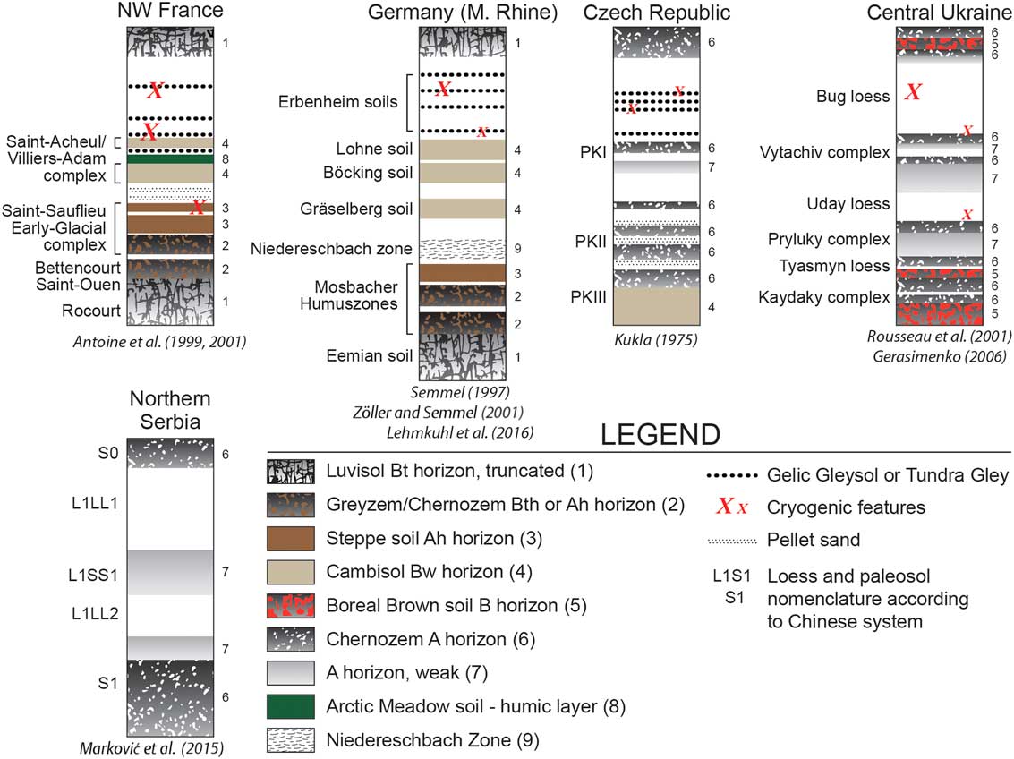
Loess in southeastern Europe is mostly found on large, broad loess plateaus, mainly in the Danube basin (Fitzsimmons et al., Reference Fitzsimmons, Marković and Hambach2012), indicating the Danube River and its tributaries were important source areas (Smalley and Leach, Reference Smalley and Leach1978; Buggle et al., Reference Buggle, Glaser, Zöller, Hambach, Marković, Glaser and Gerasimenko2008; Újvári et al., Reference Újvári, Varga and Balogh-Brunstad2008; Bokhorst et al., Reference Bokhorst, Vandenberghe, Sümegi, Lanczont, Gerasimenko, Matviishina, Markovic and Frechen2011). The Danube basin represents the largest European loess region west of the Russian/Ukrainian Plain, preserving a paleoenvironmental record extending to the Early Pleistocene (Marković et al., Reference Marković, Hambach, Stevens, Kukla, Heller, McCoy, Oches, Buggle and Zöller2011). Because of its plateau setting and the absence of periglacial influences (Fig. 5), Danube LPSs are some of the most complete, representing one of the thickest (up to >40 m), longest (since Early/Mid-Pleistocene), and most widespread terrestrial Quaternary paleoclimate archives in Europe (Fink and Kukla, Reference Fink and Kukla1977; Buggle et al., Reference Buggle, Hambach, Kehl, Marković, Zöller and Glaser2013; Marković et al., Reference Marković, Stevens, Kukla, Hambach, Fitzsimmons, Gibbard and Buggle2015). In the southern Pannonian/Carpathian basin (Hungary and Serbia) and in the lower Danube basin (Romania and Bulgaria) core data point to loess thicknesses >100 m (Pfannenstiel, Reference Pfannenstiel1950; Pécsi, Reference Pécsi1985; Koloszar, Reference Koloszar2010; Jipa, Reference Jipa2014). Unlike central and western Europe, loess here is characterized by a generally straightforward stratigraphy (Fig. 6), where stronger soil formation is related to warmer phases (usually associated with odd-numbered MISs), and loess deposition occurs mainly during colder stages (Fig. 7) (Marković et al., Reference Marković, Stevens, Kukla, Hambach, Fitzsimmons, Gibbard and Buggle2015). Despite the wide distribution of the Danube loess, the southern limit of the European loess belt interior of the Balkan Peninsula is characterized by many isolated loess deposits that originate from local sources rather than from the Danube proper. These smaller loess deposits exhibit unique geophysical and geochemical properties (Basarin et al., 2011; Obreht et al., Reference Obreht, Buggle, Catto, Marković, Bösel, Vandenberghe and Hambach2014, Reference Obreht, Zeeden, Hambach, Veres, Marković, Bösken, Svirčev, Bačević, Gavrilov and Lehmkuhl2016).
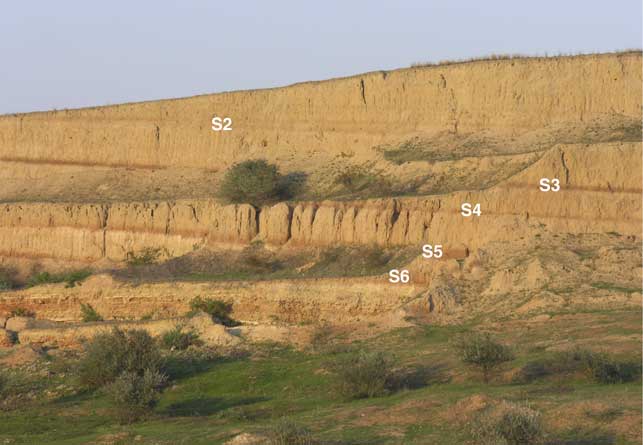
(color online) A Middle Pleistocene loess-paleosol sequence from Mircea Voda (Dobrogea, Romania). The approximately 25-m-high sequence represents the dry steppe loess facies of the lower Danube basin. Note the characteristic uppermost double paleosol (S2) that corresponds to Marine Oxygen Isotope Stage (MIS) 7, while the lowermost strongly developed paleosol (S6) represents MIS 17 (Buggle et al., Reference Buggle, Hambach, Glaser, Gerasimenko, Marković, Glaser and Zöller2009). Photo by Ulrich Hambach.

(color online) Principal stratigraphic subdivisions and important paleosols within the lithologic/loess record for the last 130 ka, for five main sites throughout Europe. Vertical scales on the diagrams are not uniform. In order to better match the graphics to the legend, each soil has been numbered, and the numbers have placed next to the stratigraphic profiles. After Marković et al. (Reference Marković, Bokhorst, Vandenberghe, Oches, Zöller, McCoy, Gaudenyi, Jovanović, Hambach and Machalett2008).

Loess in eastern Europe forms a blanket that covers an area exceeding 1 million km2. This loess was derived from the alluvial and lacustrine plains that formed in front of the advancing and retreating Pleistocene ice sheets (Velichko, Reference Velichko1990). This huge loess belt covers different bioclimatic zones, from the boreal southern taiga to the sub-Mediterranean, Black, and Azov Sea coasts, and also farther east to the Caspian Sea. Loess thickness here generally increases to the south, indicating glacial sources but also including material from local and other origins within a mixed zone in the south. Most comprehensive studies of LPSs in eastern Europe have been performed in the southern part of the East European Plain (Tsatskin et al., Reference Tsatskin, Heller, Hailwood, Gendler, Hus, Montgomery, Sartori and Virina1998; Rousseau et al., Reference Rousseau, Gerasimaenko, Matvviishina and Kukla2001, Reference Rousseau, Derbyshire, Antoine and Hatté2013; Haesaerts et al. Reference Haesaerts, Borziak, Chirica, Damblon, Koulakovska and van der Plicht2003; Velichko et al., Reference Velichko, Catto, Kononov, Morozova, Novenko, Panin and Ryskov2009; Liang et al., Reference Liang, Yang, Velichko, Zeng, Shi, Wang and Chen2016).
Loess in southwestern Europe is almost entirely concentrated in the Ebro valley and central Spain (e.g., Bertran et al., Reference Bertran, Liard, Sitzia and Tissoux2016). This loess does not reach the thicknesses of loess in central and eastern Europe and is mostly preserved as relocated loess derivates. Boixadera et al. (Reference Boixadera, Poch, Lowick and Balasch2015) reported about loess deposits that are generally 3–4 m thick and consist of well-sorted fine sands and silts (i.e., coarser than typical loess). Loess in central Spain is distributed along the Tajo River, covering fluvial terraces and depressions nearby.
Loess in midcontinent North America
By Joseph A. Mason
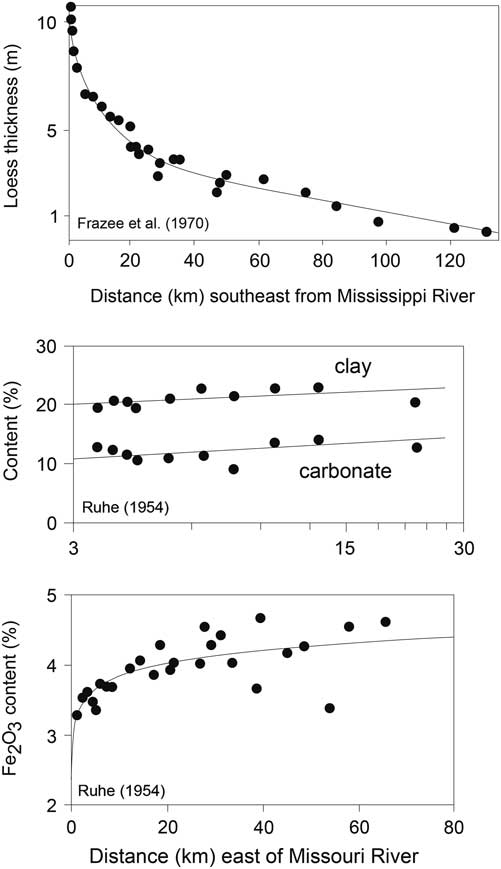
Some of the most important issues that still challenge loess researchers in the Central Lowlands and Great Plains of North America were already apparent in the classic map of eolian deposits of the United States, Alaska, and parts of Canada by Thorp and Smith (Reference Thorp and Smith1952). Drawing on extensive observations by soil surveyors and geologists, Thorp and Smith (Reference Thorp and Smith1952) mapped thick loess bordering the Mississippi, Missouri, Illinois, Wabash, and Ohio Rivers, all of which had drained the ice sheet of the last glaciation. Loess deposits exhibited well-defined thinning trends away from each river valley. A much broader swath of thick loess extended across the central Great Plains, from eastern Colorado to the Missouri River, thinning toward the southeast but with no obvious relationship to possible river valley sources (for an updated map, see Bettis et al., Reference Bettis, Muhs, Roberts and Wintle2003). Thorp and Smith (Reference Thorp and Smith1952) also accurately mapped many areas of thin loess across the Central Lowlands and Great Plains and provided a separate map of the Illinoian (Marine Oxygen Isotope Stage [MIS] 6) Loveland Loess, but their work emphasized the great thickness and extensive distribution of Late Pleistocene (MIS 2) Peoria Loess.
Today, interpretations of Peoria Loess, its sources and their paleoenvironmental controls, and its episodic and often very rapid accumulation rates, remain a central issue in midcontinent loess research. Provenance studies have revealed that much of the Peoria Loess of the central Great Plains was derived from Cenozoic rocks cropping out in unglaciated landscapes to the northwest (Aleinikoff et al., Reference Aleinikoff, Muhs, Saner and Fanning1999, Reference Aleinikoff, Muhs, Bettis, Johnson, Fanning and Benton2008; Muhs et al., Reference Muhs, Bettis, Aleinikoff, McGeehin, Beann, Skipp, Marshall, Roberts, Johnson and Benton2008b). The paleoenvironments and processes involved in this enormous amount of nonglacial dust production remain poorly understood. In contrast, much of the Peoria Loess farther east is closely linked to glacial sediments carried by the Mississippi and other rivers during MIS 2, with changing sediment availability linked to ice lobe advance and retreat (Follmer, Reference Follmer1996; Grimley, Reference Grimley2000; Bettis et al., Reference Bettis, Muhs, Roberts and Wintle2003). Peoria Loess deposits record some of the highest mass accumulation rates known worldwide, and just as interesting, improved age control—most recently through 14C dating of gastropod shells—has confirmed large changes in accumulation rate over time (Roberts et al., Reference Roberts, Muhs, Wintle, Duller and Bettis2003; Muhs et al., Reference Muhs, Bettis, Roberts, Harlan, Paces and Reynolds2013a; Pigati et al., Reference Pigati, McGeehin, Muhs and Bettis2013; Nash et al., Reference Nash, Conroy, Grimley, Guenthner and Curry2017). At present, it appears that these changes were not synchronous across the Central Lowlands or Great Plains and thus may be related to local variations in sediment supply, or changing source areas (e.g., Nash et al., Reference Nash, Conroy, Grimley, Guenthner and Curry2017) rather than broader climatic change, not surprising given the complexity of Peoria Loess sources. Geomorphic evidence also exists for large-scale deflation of coarse, source-proximal Peoria Loess, and experimental evidence suggests that there is a high potential for eolian reentrainment in the absence of vegetation cover or cohesive crusts (Sweeney and Mason, Reference Sweeney and Mason2013). These processes could also be responsible for abrupt local changes in grain size or accumulation rate.
The stratigraphy of loess, both older and younger than the Peoria Loess, emphasizes the unique nature of the loess system during MIS 2 (Mason et al., Reference Mason, Joeckel and Bettis2007) but also raises many other questions. Parts of the White River (Late Eocene-Oligocene) and Arikaree (Oligocene-Miocene) groups in western Nebraska are interpreted as volcaniclastic loess (Swinehart et al., Reference Swinehart, Souders, De Graw and Diffendal1985; Hunt, Reference Hunt1990; LaGarry, Reference LaGarry1998), helping to explain why large volumes of these rocks were later reworked into Peoria Loess (Aleinikoff et al., Reference Aleinikoff, Muhs, Saner and Fanning1999, Reference Aleinikoff, Muhs, Bettis, Johnson, Fanning and Benton2008; Yang et al., Reference Yang, Mason, Zhang, Lu, Ji, Chen and Liu2017). Loesslike silt predating the Matuyama-Brunhes (M-B) boundary at 780 ka has been identified in Illinois (Grimley and Oches, Reference Grimley and Oches2015); however, continuous loess sequences in the midcontinent apparently all postdate the M-B boundary and/or the Lava Creek B tephra (~630 ka; Matthews et al., Reference Matthews, Vasquez and Calvert2015). The relative scarcity of Early Pleistocene loess must in part reflect poor preservation, but other factors should also be explored. For example, if Early Pleistocene ice sheets extended farther south but had lower profiles (Clark and Pollard, Reference Clark and Pollard1998), the resulting glacial atmospheric circulation might not have favored dryland dust production from potential sources on the Great Plains.
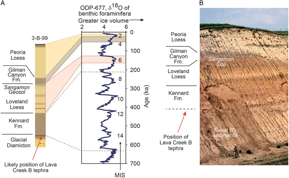
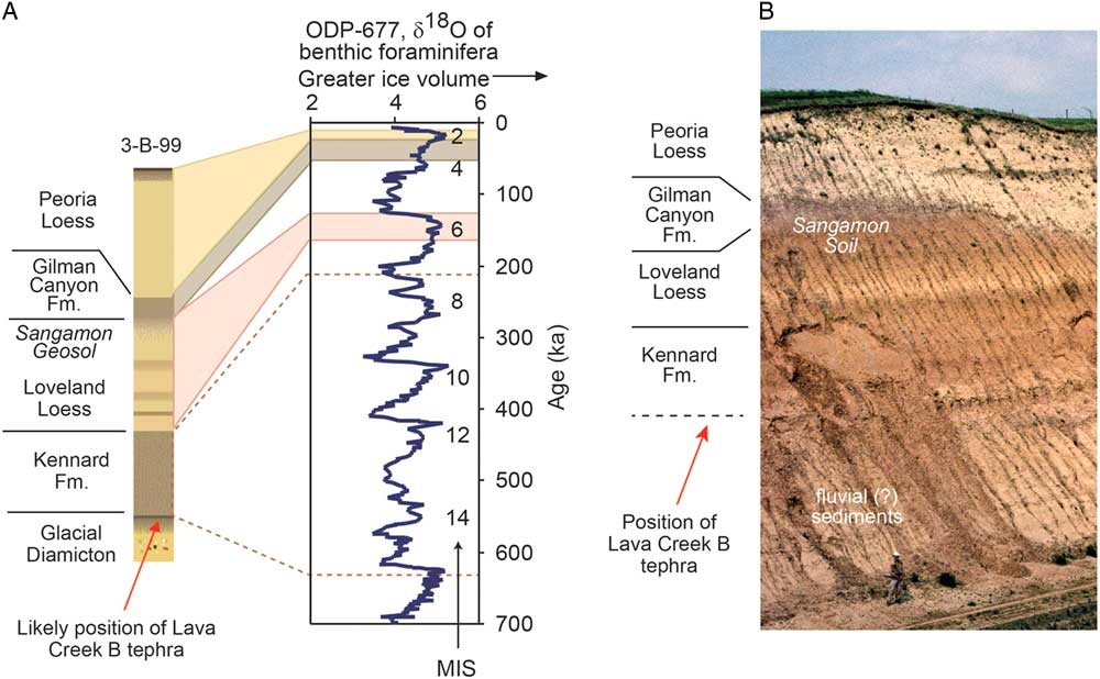
The loess sequence in eastern and central Nebraska (Fig. 8) is broadly representative of the stratigraphy of thick loess at localities across the midcontinent where preservation is high. The oldest part of this sequence includes multiple thin depositional units of the Middle Pleistocene Kennard Formation (Mason et al., Reference Mason, Joeckel and Bettis2007). The stratigraphy, chronology, provenance, and paleoenvironmental record of the Kennard Formation remain largely unstudied, as have possible correlations with pre–Loveland Loess units reported from scattered localities along the Mississippi River valley (Porter and Bishop, Reference Porter and Bishop1990; Jacobs and Knox, Reference Jacobs and Knox1994; Leigh and Knox, Reference Leigh and Knox1994; Grimley, Reference Grimley1996; Rutledge et al., Reference Rutledge, Guccione, Markewich, Wysocki and Ward1996; Markewich et al., Reference Markewich, Wysocki, Pavich, Rutledge, Millard, Rich, Maat, Rubin and McGeehin1998). A variety of evidence indicates the overlying Loveland Loess was deposited during the MIS 6 glacial period, although luminescence ages at some sites suggest the uppermost part may be younger (Forman et al., Reference Forman, Bettis, Kemmis and Miller1992; Maat and Johnson, Reference Maat and Johnson1996; Rodbell et al., Reference Rodbell, Forman, Pierson and Lynn1997; Markewich et al., Reference Markewich, Wysocki, Pavich, Rutledge, Millard, Rich, Maat, Rubin and McGeehin1998; Forman and Pierson, Reference Forman and Pierson2002; Grimley and Oches, Reference Grimley and Oches2015). An intriguing characteristic of thick Loveland Loess is the presence of a lower, darker-colored zone, which may contain multiple weak paleosols, suggestive of slow and/or intermittent deposition (Grimley, Reference Grimley1996; Mason et al., Reference Mason, Joeckel and Bettis2007). Above the prominent Sangamon Soil, which caps the Loveland Loess and developed through MIS 5 and 4, is an MIS 3 loess unit variously known as the Roxana Silt (Mississippi valley), Pisgah Loess (Iowa), or Gilman Canyon Formation (Great Plains). It has characteristics similar to the lower Loveland Loess; 14C and luminescence dating confirms its slow accumulation rate (Leigh, Reference Leigh1994; Follmer, Reference Follmer1996; Markewich et al., Reference Markewich, Wysocki, Pavich, Rutledge, Millard, Rich, Maat, Rubin and McGeehin1998; Bettis et al., Reference Bettis, Muhs, Roberts and Wintle2003; Johnson et al., Reference Johnson, Willey, Mason and May2007; Muhs et al., Reference Muhs, Bettis, Roberts, Harlan, Paces and Reynolds2013a). This similarity suggests the lower zone of Loveland Loess on the Great Plains could preserve an isotopic record of shifting dominance by C3 and C4 grassland, as does the Gilman Canyon Formation (Johnson et al., Reference Johnson, Willey, Mason and May2007). Above the MIS 3 loess, Peoria Loess accumulated between about 28 ka and 13 ka (MIS 2) across the midcontinent, with the exact time span varying regionally and possibly locally (Bettis et al., Reference Bettis, Muhs, Roberts and Wintle2003; Muhs et al., Reference Muhs, Bettis, Roberts, Harlan, Paces and Reynolds2013a; Pigati et al., Reference Pigati, McGeehin, Muhs and Bettis2013; Nash et al., Reference Nash, Conroy, Grimley, Guenthner and Curry2017). On the central Great Plains and along the Missouri River valley in North and South Dakota, the loess record continues into the Holocene. The Brady Soil, formed during a period of limited dust accumulation between about 14 and 10 ka, is sometimes found in the upper Peoria Loess, when Bignell Loess overlies it. Where the latter is thick, it represents a high-resolution record of Holocene dust deposition (Johnson and Willey, Reference Johnson and Willey2000; Mason et al., Reference Mason, Jacobs, Hanson, Miao and Goble2003, Reference Mason, Miao, Hanson, Johnson, Jacobs and Goble2008). The specific geomorphic mechanisms of Holocene dust production, downwind dispersal, and patchy retention in the landscape, and their connections to changing climate and vegetation, are worthy of additional study because of their potential relevance to the environmental changes associated with a warmer and drier future climate.
(color online) (A) The general loess stratigraphy found in eastern Nebraska, USA, as represented by core 3-B-99 (41°29′N, 96°13′W) (Mason et al., Reference Mason, Joeckel and Bettis2007). Peoria Loess, Gilman Canyon Formation, and Loveland Loess are correlated with specific parts of marine isotope record based on numerical dating. Ages assigned to Loveland Loess are based on luminescence dating at the paratype locality in western Iowa (Forman and Pierson, Reference Forman and Pierson2002); ages assigned to Kennard Formation are based on its stratigraphic position between Loveland Loess and Lava Creek B tephra, supported by burial dating of Balco et al. (Reference Balco, Stone and Mason2005). MIS, Marine Oxygen Isotope Stage. (B) Loess stratigraphy in the Elba Cut section of central Nebraska (41°18′N, 98°31′W), interpreted by J. Mason by comparison with eastern Nebraska sections (Mason et al., Reference Mason, Joeckel and Bettis2007). Note person at base of section for scale. The tephra present in this section (to left of area shown here) is the Lava Creek B (E.A. Bettis III, personal communication 2006).
Loess in Alaska
By E. Arthur Bettis III
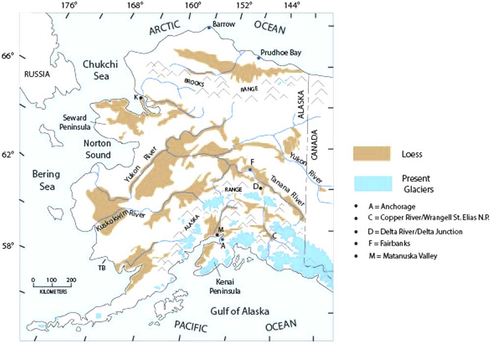
Loess associated with glacigenic valley-train sources is extensive over much of Alaska and adjacent parts of adjacent Yukon Territory in Canada (Fig. 9). In some parts of central Alaska, loess can be as much as several tens of meters thick and, based on a combined tephra and paleomagnetic record, may date back as far as the onset of North American glaciation, ~3 Ma (Westgate et al., Reference Westgate, Stemper and Péwé1990). It was not until the mid-1950s that the extensive deposits of silt on the Alaskan landscape were properly recognized as loess. Prior to that time, some researchers regarded them as the result of frost shattering or other processes (Taber, Reference Taber1943, Reference Taber1953, Reference Taber1958). It was Péwé (Reference Péwé1955), however, who finally brought together several converging lines of evidence--geomorphic, stratigraphic, and mineralogical—that established that these silt bodies in Alaska are loess. Loess is now recognized over many parts of the region, including a broad area of the coastal plain north of the Brooks Range, over parts of the Seward Peninsula (Hopkins, Reference Hopkins1963), in the Yukon River basin (Williams, Reference Williams1962; Begét et al., Reference Begét, Edwards, Hopkins, Keskinen and Kukla1991; Jensen et al., Reference Jensen, Reyes, Froese and Stone2013), in the Tanana River valley and along the Delta River valley of central Alaska (Péwé, Reference Péwé1955, Reference Péwé1975; Muhs et al., Reference Muhs, Ager, Bettis, III, McGeehin, Been, Begét, Pavich, Stafford and Stevens2003b), in southern Alaska in the Matanuska Valley (Muhs et al., Reference Muhs, McGeehin, Beann and Fisher2004, Reference Muhs, Budahn, Skipp and McGeehin2016), on the Kenai Peninsula (Reger et al., Reference Reger, Pinney, Burke and Wiltse1996), and along the Copper River valley in Wrangell–St. Elias National Park (Muhs et al., Reference Muhs, Budahn, McGeehin, Bettis, Skipp, Paces and Wheeler2013b; Pigati et al., Reference Pigati, McGeehin, Muhs and Bettis2013).
(color online) Map of Alaska showing the distribution of Quaternary loess deposits and the distribution of modern glaciers. Lettered dots refer to localities discussed in the text. After Muhs et al. (Reference Muhs, Ager, Bettis, III, McGeehin, Been, Begét, Pavich, Stafford and Stevens2003b).

Loess deposits in Alaska that have been securely dated to the last glacial period are elusive or are very thin. On the Seward Peninsula, less than a meter of loess blankets a land surface with fossil tundra vegetation that dates to the last glacial period (Höfle and Ping, Reference Höfle and Ping1996; Höfle et al., Reference Höfle, Edwards, Hopkins and Mann2000). In the Fox Permafrost Tunnel near Fairbanks, loess that is bracketed by a radiocarbon age of ~9.5 ka above and ~34 ka below could date to the last glacial period (Hamilton et al., Reference Hamilton, Craig and Sellmann1988), as is the case for very thin loess dated between ~12 ka and ~36 ka nearby in an upland locality (Muhs et al., Reference Muhs, Ager, Bettis, III, McGeehin, Been, Begét, Pavich, Stafford and Stevens2003b). In neither of these two cases, however, is loess dated directly to the last glacial period. Attempts to date other last-glacial central Alaskan loess deposits have been frustrated by a lack of materials suitable for radiocarbon analyses or uncertainties in luminescence geochronology (Oches et al., Reference Oches, Banerjee, Solheid and Frechen1998; Berger, Reference Berger2003; Muhs et al., Reference Muhs, Ager, Been, Bradbury and Dean2003a; Auclair et al., Reference Auclair, Lamothe, Lagroix and Banerjee2007). However, recent identification of the Dawson tephra (~30 ka) in the upper part of loess deposits near Fairbanks permits an interpretation of as much as ~3 m of accumulation since the time of tephra deposition (Jensen et al., Reference Jensen, Evans, Froese and Kravchinsky2016). Nevertheless, it is not known how much of this sediment is of last-glacial age and how much may be of Holocene age.
Older, pre–last-glacial loesses are well documented in Alaska. The chronology of these older loesses has been aided immeasurably by detailed studies of tephras that are interbedded with the eolian silts (Westgate et al., Reference Westgate, Stemper and Péwé1990; Begét et al., Reference Begét, Edwards, Hopkins, Keskinen and Kukla1991; Preece et al., Reference Preece, Westgate, Stemper and Péwé1999; Jensen et al., Reference Jensen, Reyes, Froese and Stone2013, Reference Jensen, Evans, Froese and Kravchinsky2016). Jensen et al. (Reference Jensen, Evans, Froese and Kravchinsky2016) described evidence for significant pre–last-glacial loess accumulation in central Alaska during Marine Isotope Stages 4 and 6, with accumulation rates greatest during transitions between isotope stages. Furthermore, these investigators noted that in the middle and early Pleistocene, glaciations were much more extensive in Alaska than during the last glacial period (Kaufman et al., Reference Kaufman, Manley, Ager, Axford, Balascio, Begét and Brigham-Grette2004), which likely enhanced the supply of glaciogenic silt available for loess accumulation.
Whereas loess dated to the last glacial period has been elusive in Alaska, there are abundant loess bodies that date to the Holocene, and deposition continues today in many parts of the region. In the Delta Junction area of central Alaska, only Holocene loess has been documented (Péwé, Reference Péwé1975; Muhs et al., Reference Muhs, Ager, Bettis, III, McGeehin, Been, Begét, Pavich, Stafford and Stevens2003b). On the Kenai Peninsula of southern Alaska, the Lethe tephra dating to ~19 ka to ~15 ka is found below, or in the lower part of loess, but as on the Seward Peninsula, this eolian silt is less than a meter thick (Reger et al., Reference Reger, Pinney, Burke and Wiltse1996). Elsewhere in southern Alaska, near Anchorage, loess of the Matanuska Valley all dates to the Holocene (Muhs et al., Reference Muhs, McGeehin, Beann and Fisher2004, Reference Muhs, Budahn, Skipp and McGeehin2016), as does loess of the Copper River valley in Wrangell–St. Elias National Park, to the east (Muhs et al., Reference Muhs, Budahn, McGeehin, Bettis, Skipp, Paces and Wheeler2013b; Pigati et al., Reference Pigati, McGeehin, Muhs and Bettis2013).
Paleosols intercalated in loess sequences have long been the focus of study, for stratigraphy, geochronology, and paleoenvironmental interpretation in most loess regions. In Alaska, however, little mention of paleosols in the loess sequence was made by geologists until relatively recently. Indeed, some researchers even doubted their existence (Péwé et al., Reference Péwé, Berger, Westgate, Brown and Leavitt1997). Begét and his colleagues at the University of Alaska were the first to bring the geologic community’s attention to the rich record of paleosols in Alaskan loess in a landmark series of papers (Begét and Hawkins, Reference Begét and Hawkins1989; Begét, Reference Begét1990; Begét et al., Reference Begét, Stone and Hawkins1990). Paleosol research in Alaska and adjacent Yukon Territory since the time of these pioneering studies has provided new insights into the paleoenvironment during periods of reduced loess accumulation (Sanborn et al., Reference Sanborn, Smith, Froese, Zazula and Westgate2006; Muhs et al., Reference Muhs, Ager, Skipp, Beann, Budahn and McGeehin2008a).
Loess in Argentina, South America
By Marcello Zárate and Alfonsina Tripaldi
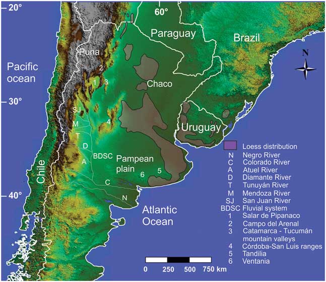
The loess deposits of southern South America cover broad areas of the eastern Pampean plain of Argentina, southern Brazil, and Uruguay, as well as several areas of the Chaco region, and mountain valleys of the northwestern Pampean ranges (Fig. 10). The focus of this overview is on the loess deposits in Argentina. In the Pampean region of Argentina, loess and loesslike deposits range in age from the late Miocene through the Quaternary; in some Pampean areas, loess accumulation even continued until the early–mid-Holocene. Luminescence chronology carried out in the extensive apron of the last-glacial loess suggests regional variation in depositional rates over this interval, with relatively high accumulation rates during the last glacial maximum and the late glacial intervals. The average thickness of the last-glacial Pampean loess is ~1.5–2 m, with up to 3–4 m in the mountains surrounding the Pampean plain (i.e., the Tandilia and Ventania ranges and the Pampean ranges of Córdoba-San Luis). Sandy eolian deposits (dune fields, sand sheets) dominate in the western-southwestern Pampean plain and grade into loess mantles downwind (Zárate and Tripaldi, Reference Zárate and Tripaldi2012). The loess deposits also show a gradual grain-size decrease from silty fine sands to silty deposits in the eastern Pampean plain (González Bonorino, Reference González Bonorino1966). The mineralogical assemblage of the Pampean loess is dominantly composed of plagioclase, volcanic shards (both fresh and weathered), quartz, K-feldpars, and fragments of basalt, andesite, and rhyolite. Magnetite, amphibole, and pyroxene, among others, are the most common heavy minerals. The direct input of Andean volcanic eruptions in the loess deposits is documented by fresh volcanic shards, whereas most of the loess grains were derived from the erosion and fluvial transportation of extensive volcaniclastic units (sensu Fisher, Reference Fisher1961) exposed in the Andes Cordillera and its piedmont. These volcaniclastic units comprise late Miocene to Quaternary fine-grained pyroclastic deposits, and volcanic rocks (basalts, andesites), as well as lower Mesozoic acid volcanic rocks (González Bonorino, Reference González Bonorino1966). The origin of the volcaniclastic sedimentary sand and silt particles has been attributed to explosive volcanism (Zárate and Blasi, Reference Zárate and Blasi1993) and physical weathering (Iriondo, Reference Iriondo1990). Secondary loess sources, including the Brazilian plateau, the Tandilia and Ventania ranges, and the Pampean ranges surrounding the Pampean plain, have also been documented and show variable contributions, according to the area considered (Zárate and Tripaldi, Reference Zárate and Tripaldi2012). The eolian sand and silt particles are thought to have been deflated by west–southwest winds from the fluvial system of (1) the Bermejo-Desaguadero-Salado-Curacó (BDSC) River (Iriondo, Reference Iriondo1990), a wide depositional system at the distal eastern piedmont of the Andes, and (2) the Colorado-Negro Rivers (Zárate and Blasi, Reference Zárate and Blasi1993), where volcaniclastic sediments are abundant. Northeast–southeast winds prevailed along the northern extent of the BDSC system, between the Diamante and San Juan Rivers, and the western Pampas near the San Luis ranges (Fig. 10), where eolian sandy sediments document a mixed provenance, including volcaniclastic, metamorphic, and igneous rocks from the surrounding Pampean ranges (Zárate and Tripaldi, Reference Zárate and Tripaldi2012). In order to improve our understanding of Quaternary eolian systems, most current research has focused on two main topics related to the loess here: (1) investigation of the sedimentary environments of the source area represented by the BDSC fluvial system and (2) Quaternary loess deposits of the northwestern mountain valleys.
(color online) DEM (Digital Elevation Model) image of southern South America with general location of the Pampean plain, Chaco, Puna, and other areas discussed in the text. Localities referred to in the text are keyed to the legend in the lower right of the figure.

Studies in progress suggest that the BDSC fluvial system is a complex sedimentary setting consisting of major alluvial fans generated by its main tributaries (i.e., the San Juan, Mendoza, Tunuyán, Atuel, and Diamante Rivers), all of which drain eastward, out of the Andes Mountains. General paleoclimatological and paleoenvironmental reconstructions suggest that arid and arid-semiarid conditions dominated here during the accumulation of the alluvial deposits (i.e., from the late Pleistocene to the present; Mancini et al., Reference Mancini, Paez, Prieto, Stutz, Tonello and Vilanova2005). The San Juan, Mendoza, Tunuyán, Atuel, and Diamante drainage basins have a seasonal precipitation regime, with winter snowfalls generated by the Pacific cyclones, in their upper basins. These areas were also glaciated (Espizúa, Reference Espizúa2004), promoting increased seasonal discharges during the Pleistocene. Sedimentologic analysis focused on the lower basins of the Atuel and Diamante Rivers has documented a large alluvial fan (200 km long and 100 km wide) dominated by fine sand/coarse silt deposits. Diverse sedimentary settings, including numerous channels and their associated floodplains, as well as shallow saline lakes, are reported for this system, along with extensive eolian deposits (dunes and sand sheets) covering large parts of the alluvial deposits (Lorenzo et al., Reference Lorenzo, Mehl and Zárate2017; Tripaldi and Zárate, Reference Tripaldi and Zárate2017). Farther north, in Catamarca Province, loess deposits have been recently explored in a valley situated ~100 km southwest of the Tafí del Valle loess locality of Tucumán (Stiglitz et al., Reference Stiglitz, Banerjee, Gourlan and Oches2006). The loess deposits here are up to 40 m thick and include interlayered fluvial sediments and paleosols. Loess has also been reported nearby, covering the planation surface of the Ancasti Pampean range (Sayago, Reference Sayago1983). Immediately west of the Catamarca valley are large intermountain tectonic basins (e.g., the Salar de Pipanaco, Campo del Arenal) that contain fine alluvial sands and silts from rivers that drain the Andes and the Puna region and their associated dune fields.
Although several areas still remain unexplored and/or poorly investigated, current studies allow for a reinter-pretation of the BDSC fluvial system as a large bajada resulting from the north–south coalescence of several major alluvial fans generated by rivers with highly seasonal flow regimes from winter snowfalls and glaciers, under generally arid-semiarid conditions. This depositional environment has abundant sand and silt, derived from the erosion of late Cenozoic volcanic rocks and pyroclastic deposits, and older volcanic and volcaniclastic units exposed in the Andes and the eastern piedmont, as well as metamorphic and igneous rocks from the surrounding Pampean ranges. These sediments were subject to entrainment by prevailing west–southwest winds in the southern part of the BDSC fluvial system, and northeast–southeast winds in the northern part.
Two important questions remain regarding the source area of the northwestern mountain valley loess of Catamarca: (1) What were the prevailing wind directions? (2) Has this loess been deflated from the tectonic basins located to the west-northwest, or did it originate via high suspension from more distal environments (i.e., the Puna plateau)? Future research should include a more detailed analysis of the late Quaternary eolian deposits in the northern BDSC system that may show a mixed provenance, and that may have been derived from northeast–southeast winds, as well as the loess deposits of the northwestern mountain valleys. These studies may help discern the role played by regional and/or local factors during the eolian accumulation phases in this region.
Loess at desert margins
By Onn Crouvi
Loess at desert margins (termed here as “desert loess”) refers to eolian silt deposits generated in, and derived from, nonglaciated, low-latitude warm-arid or semiarid regions. The documentation of loess at desert margins since the mid-twentieth century (e.g., Yaalon, Reference Yaalon1969; Coude-Gaussen, Reference Coude-Gaussen1987; McTainsh, Reference McTainsh1987) has confounded the traditional view of silt generation solely by glacial grinding (e.g., Smalley and Krinsley, Reference Smalley and Krinsley1978) that is widely attributed to most of the world’s well-known loess deposits. Thus, a number of nonglacial processes that produce silt grains in deserts have long been proposed and debated (e.g., Smalley, Reference Smalley1995; Assallay et al., Reference Assallay, Rogers, Smalley and Jefferson1998; Wright, Reference Wright2001; Smith et al., Reference Smith, Wright and Whalley2002; Muhs and Bettis, Reference Muhs and Bettis2003), including salt weathering, frost weathering, deep weathering, fluvial comminution, and eolian abrasion.
Desert loess is known to exist at the margins of deserts in Africa (Tunisia, Libya, Algeria, Nigeria, and Namibia), in the Middle East (Israel, Yemen, the United Arab Emirates, and Iran), the western United States, the Great Plains of North America, and Australia (Fig. 11A). With the exception of the thick nonglacial loess in the Great Plains of North America, loess of this kind is patchy and varies in thickness from a few meters on uplands to a few tens of meters in valleys. Importantly, desert loess is the parent material for some of the most fertile soils in these regions. A few characteristics are common to all reported desert loess sites in Africa and the Middle East (Crouvi et al., Reference Crouvi, Amit, Enzel and Gillespie2010): (1) loess sediments are dominantly coarse silt to very fine sand, with median grain sizes ranging from 50 to 80 µm, and at some sites, the particle-size distribution is reported to be tri- or bimodal; (2) loess mineralogy is mostly quartz and feldspars, with various amounts of carbonate, depending on the degree of soil development in the loess; (3) at most sites, the underlying lithologies are inconsistent with the presence of quartz in the loess, suggesting an external silt source; (4) the shapes of loess particles are reported as subangular to angular for most regions; and (5) most loess bodies were deposited during the last glacial period (~110–10 ka). Crouvi et al. (Reference Crouvi, Amit, Enzel and Gillespie2010) noted that all these loess regions are located only a few tens of kilometers downwind from sand dunes (Fig. 11), and based on the mineralogical, spatial, and temporal associations between these two eolian bodies, suggested that the proximal source of the coarse silt in loess is the upwind dunes, via eolian abrasion of sand grains.
(color online) (A) Spatial distribution of loess in Africa and Arabia, active sand seas, and Arenosols (sandy soils) (Food and Agriculture Organization of the United Nations, International Institute for Applied Systems Analysis, ISRIC–World Soil Information, Institute of Soil Science–Chinese Academy of Sciences, and Joint Research Centre of the European Commission, 2009). Near surface dominant wind directions for January and June are based on Breed et al. (Reference Breed, Fryberger, Andrews, McCauley, Lennartz, Gebel and Horstman1979). Silt (content in %, 24 µm mode) in oceanic sediments off the coast of West Africa deposited during the last glacial maximum (Sarnthein et al., Reference Sarnthein, Tetzlaff, Koopmann, Wolter and Pflaumann1981). See text for further details on the Negev loess, Israel. After Crouvi et al. (Reference Crouvi, Amit, Enzel and Gillespie2010). (B) Map of Israel and its surroundings, showing the distribution of sand dunes (white polygons with black dots) and loessial (dark gray) and sandy (light gray) soils in the Negev and Sinai deserts (the soils were mapped only in Israel). Mean annual rainfall (mm) in Israel for the period 1961–1990 is shown by dashed isohyets. Black arrows are the inferred westerly winds prevalent during sand incursion. Insert shows the location of Israel in the eastern Mediterranean region and the mean annual rainfall isohyets (mm). After Crouvi et al. (Reference Crouvi, Amit, Enzel, Porat and Sandler2008).

The Negev loess (Israel) is one of the world’s best-studied desert loess deposits, with scientific exploration that goes back to the early twentieth century (Fig. 11B; see Crouvi et al, Reference Crouvi, Amit, Ben Israel and Enzel2017a). The carbonate bedrock lithology of the Negev and its physiography provide a unique opportunity to understand the sources of this silicate-rich loess and to explore silt formative processes in deserts. Grain-size data from the Negev loess have three main characteristics: (1) clear textural bimodality, with one mode in the coarse silt fraction (36–65 µm) and another in the fine silt to clay fraction (2.5–10 µm); (2) grain-size decreases to the north, east, and south, away from the sand dunes that border the loess deposit on the west; and (3) increasing grain-size upward in each individual primary sequence. Recognizing the bimodality of the loess, Dan Yaalon was the first to suggest that the Negev loess had two different sources that supplied sediments through two different transport pathways (Yaalon, Reference Yaalon1969; Yaalon and Ganor, Reference Yaalon and Ganor1973, Reference Yaalon and Ganor1979; Yaalon and Dan, Reference Yaalon and Dan1974): distal sources in the Sahara and Arabia deserts supplying fine silt and clays transported by cyclonic winds over thousands of kilometers, and proximal sources in Sinai, such as Wadi El-Arish in northern Sinai, supplying the coarser silts. However, recent studies have shown that the major source of the coarse silt grains is the adjacent, upwind sand dunes that advanced into Sinai and Negev during the late Pleistocene, concurrent with accumulation of the loess (Crouvi, Reference Crouvi2009; Crouvi et al., Reference Crouvi, Amit, Enzel, Porat and Sandler2008). This conclusion was based on the following observations: (1) increases of the quartzofeldspathic coarse mode upward in the loess deposits, (2) the spatiotemporal association of sand dune activities and dust mass accumulation rates (MARs) of the loess, (3) similarity in mineralogical composition and in isotopic composition of Sr and Nd between the sand dunes and the coarse fraction of the loess (Muhs et al., Reference Muhs, Roskin, Tsoar, Skipp, Budahn, Sneh, Porat, Stanley, Katra and Blumberg2013c; Ben Israel et al., Reference Ben Israel, Enzel, Amit and Erel2015), and (4) location—the loess was located downwind of sand dunes during the late Pleistocene, as evident by the linear orientation of the dunes. In addition, recent studies have shown that the quartz-rich silt fraction in soils in the Judean Mountains and their lowlands, north of the loess, can be regarded as the direct continuation of the dune – loess association (Crouvi et al., Reference Crouvi, Barzilai, Goldsmith, Amit, Porat and Enzel2014; Amit et al., Reference Amit, Enzel and Crouvi2016). Because of the fact that these silt grains are farther away from their source than the Negev loess deposits, they are finer-grained and exhibit lower MARs. Finally, because much of the Negev loess formed during the late Pleistocene, it has been undergoing erosion through most of the Holocene, and even more severely during the last 100 yr because of agriculture practices. The erosion is both by water (e.g., Avni, Reference Avni2005; Avni et al., Reference Avni, Porat, Plakht and Avni2006) and by wind (e.g., Tanner et al., Reference Tanner, Katra, Haim and Zaady2016; Crouvi et al., Reference Crouvi, Dayan, Amit and Enzel2017b), transferring the loess into a relatively young and new proximal dust source. Overall, the Negev loess can be regarded today as nonreplenishable natural resource that is slowly disappearing.
One of the main challenges in studies of loess at desert margins is the lack of comprehensive quantitative information about loess properties and their period(s) of formation (e.g., in Yemen, Namibia, and the United Arab Emirates). In other areas, there is no published map of loess distribution, and our knowledge originates mainly from sporadic documentation of the soils and sediments (e.g., the loess belt in the Sahel) and, except for the Nigerian loess, is poorly documented (see Crouvi et al., Reference Crouvi, Amit, Enzel and Gillespie2010 for more details).
Questions, challenges, and opportunities unique to loess at desert margins can be grouped into four categories: (1) Sources—despite great advances in grain-size end member modeling, and other approaches, separating between proximal and distal sources of the loess and identifying them is still an ongoing challenge. This dilemma is related to the century-old debate on the formation mechanisms of silts in deserts. (2) Paleoclimatological reconstruction—loess is an excellent climate archive that can shed light on (a) regional environmental changes, such as the appearance and disappearance of dust sources, (b) regional changes in wind direction and strength, and (c) local climate properties (i.e., precipitation), through analyzing buried soils. These reconstructions are still poorly constrained from most desert loess regions in the world. (3) The continuation of loess downwind, beyond the major deposits, is unclear. What is the effect of loess and its derivatives on the areas and soils located farther downwind? How have additions of fine silt and clay affected the soils here? (4) Loess probably presents a new and intensive dust source that might affect future climate changes. The magnitude and frequency of dust emissions from desert loess regions is still poorly documented.
METHODOLOGICAL APPROACHES TO THE STUDY OF LOESS
Loess and paleosol stratigraphy
By Slobodan B. Marković
Loess covers huge parts of the continents, from currently subtropical areas to subpolar regions. The formation of loess is often not a recent or contemporary process. Instead, loess is usually deposited under extreme conditions ranging from desert to tundralike environments associated with previous glacial phases during the Quaternary period. During these periods, complex natural processes related to the formation, production, and deposition of dust facilitated the formation of loess deposits.
Loess, which is a mixture of different minerals, represents an almost ideal substrate for soil formation. Even slight climate changes are able to initiate rapid soil formation in loess deposits. Thus, even slight shifts from periods of dust accumulation to pedogenesis can be recorded in loess; paleosols within these sequences are some of the most sensitive continental archives of environmental responses to Quaternary climate change. From this point of view, each typical loess deposit or strongly developed pedocomplex can be regarded as a basic climatostratigraphic unit, representing full glacial or interglacial conditions. Other varieties of loess derivates and weakly developed paleosols in loess are equivalent to stadial and interstadial environments, respectively.
Consequently, it is no surprise that climatostratigraphic research in many loess regions has a long and distinguished history. Many such early loess stratigraphic models represented climatostratigraphic approaches (e.g., Marković et al., Reference Marković, Fitzsimmons, Sprafke, Gavrilovic, Smalley, Jovic, Svirčev, Gavrilov and Bešlin2016). Nonetheless, they had shortcomings. Developed at the beginning of the twentieth century, many of these studies were highly speculative, and the nomenclatures used were usually derived from local place names. With the purpose of creating a common European loess stratigraphy, the Loess Subcommission (currently Loess Focus Group) of the International Union for Quaternary Research promoted pedostratigraphic criteria as the primary basis for stratigraphic correlations (Fink, Reference Fink1962; Smalley et al., Reference Smalley, Marković and O’Hara-Dhand2010). This concept culminated in the studies of Bronger and coworkers, who presented their attempts at Eurasian continental loess correlation in a series of papers (Bronger, Reference Bronger1976, Reference Bronger2003; Bronger and Heinkele Reference Bronger and Heinkele1989; Bronger et al., Reference Bronger, Winter and Sedov1998). Later, investigation of Czechian and Austrian loess exposures provided the background for correlation of terrestrial loess deposits with the oscillations recorded in deep-sea sediments, given that both likely reflect global paleoclimate drivers (Kukla, Reference Kukla1975, Reference Kukla1977; Fink and Kukla, Reference Fink and Kukla1977). The glacial cycle concept that Kukla applied to loess-paleosol sequences promoted loess as the most important terrestrial archive of Pleistocene climatic and environmental changes.
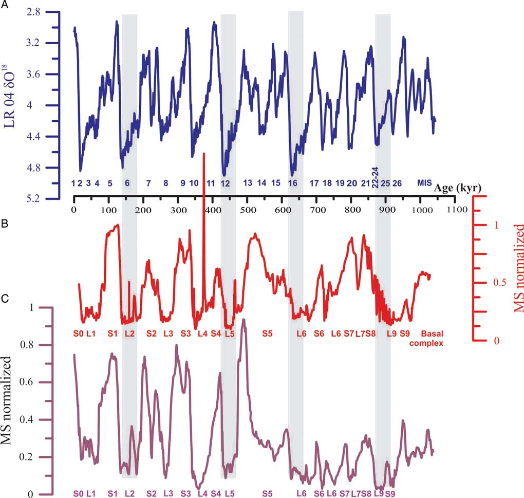
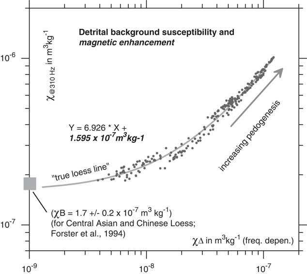
Further development of magnetostratigraphic techniques, as applied to loess in China, highlighted scientific interest in the multiple loess-paleosol couplets of the Chinese Loess Plateau (Heller and Liu, Reference Heller and Liu1982, Reference Heller and Liu1984; Liu, Reference Liu1985). This new approach, based on paleomagnetic polarity zonation, allowed for direct correlations between profiles using loess-paleosol magnetic susceptibility variations and its correspondence with Marine Oxygen Isotope Stage (MIS) stratigraphy. Eventually, this method became the basis for the famous so-called “L&S” (loess and soil) Chinese loess stratigraphic model (Liu, Reference Liu1985; Kukla, Reference Kukla1987; Kukla and An, Reference Kukla and An1989; Hao et al., Reference Hao, Wang, Oldfield, Peng, Qin, Song, Xu, Qiao, Bloemendal and Guo2012). Enhancement of the magnetic signal attributable to pedogenic processes appears to be valid for loess strata across the vast Eurasian semiarid loess zone as well (Maher and Thompson, Reference Maher and Thompson1992), further extending its application (Fig. 12). Data on loess magnetic susceptibility have since proved to be a rapid and consistent tool for interprofile correlations, even over very long distances (Marković et al., Reference Marković, Stevens, Kukla, Hambach, Fitzsimmons, Gibbard and Buggle2015). Figure 13 shows the remarkable accordance between Serbian and Chinese loess stratigraphies. The loess magnetic record from Siberian and Alaskan loess provinces has the opposite trends—that is, higher magnetic susceptibility values characterize loess deposits, with lower values in paleosols (e.g., Begét, Reference Begét1990, Reference Begét1996; Begét et al., Reference Begét, Stone and Hawkins1990; Heller and Evans, Reference Heller and Evans1995; Chlachula et al., Reference Chlachula, Evans and Rutter1998). Additional quantitative chronological approaches, such as current improvements in amino acid racemization, relative geochronology, tephrochronology, and 14C and luminescence dating, have helped to significantly improve the accuracy of loess stratigraphic models, but still only at the level of correlation with the main MISs. In the United States, most of the loess is younger than Middle Pleistocene in age, and therefore, “classic” regional loess stratigraphic models supported by luminescence and radiocarbon dating are generally more useful for long-range correlations than are data on magnetic susceptibility or amino acid racemization (Bettis et al., Reference Bettis, Muhs, Roberts and Wintle2003).
(color online) The Mircea Voda loess section in Dobrogea, Romania, is a good example of alternations of loess layers (from L1 to L5) and peodological horizons, or paleosols (from S0 to S5). These data are additionally illustrated by variations in magnetic susceptibility ranging from low values in loess units to high values in paleosols (Buggle et al., Reference Buggle, Hambach, Glaser, Gerasimenko, Marković, Glaser and Zöller2009; Timar-Gabor et al., Reference Timar-Gabor, Vandenberghe, Vasiliniuc, Panaoitu, Panaiotu, Dimofte and Cosma2011).

(color online) Direct comparisons between the marine LR04 stack (Lisiecki and Raymo, Reference Lisiecki and Raymo2005) (A) and Serbian loess (Marković et al., Reference Marković, Stevens, Kukla, Hambach, Fitzsimmons, Gibbard and Buggle2015) (B) and Chinese loess (Sun et al., Reference Sun, Clemens, An and Yu2006) (C) magnetic susceptibility (MS) records plotted on time scale. MIS, Marine Oxygen Isotope Stage.

Loess stratigraphy in the Southern Hemisphere has been investigated less intensively in South America where there is a high diversity of loess and loesslike deposits as a consequence of quite diverse environmental responses to climate forcing (Zárate, Reference Zárate2003; Iriondo and Kröhling, Reference Iriondo and Kröhling2007). An additional problem in some regions is similar to the examples mentioned previously for Siberian and Alaskan loess; in this case, the variation in magnetic susceptibility is because of contributions of volcanic material in the loess deposits (e.g., Ruocco, Reference Ruocco1989; Heller and Evans, Reference Heller and Evans1995). Similar conditions occur in New Zealand, although here the presence of many (dated) tephra layers became an important advantage for the establishment of loess stratigraphy (Palmer and Pillans, Reference Palmer and Pillans1996; Roering et al., Reference Roering, Almond, Tonkin and McKean2002).
Using the L&S stratigraphic nomenclature, already well accepted for Chinese and Danubean stratigraphic units, can be a useful global approach. The L&S stratigraphic scheme has led to standardized, regionally specific stratigraphies of European loess deposits. The L&S scheme also offers a potential for correlating the confusing diversity of European loess stratigraphic records across the Eurasian loess belt and into central Asia and China (Marković et al., Reference Marković, Stevens, Kukla, Hambach, Fitzsimmons, Gibbard and Buggle2015). In order for the L&S system to provide accurate correlations, three conditions need to be met: (1) numerical ages or tie lines to numerical ages (e.g., volcanic ash dated elsewhere) need to be available; (2) absence of unconformities in undated portions of the sections must be demonstrated; and (3) there must be an assumption that global (or at least continental) geoenvironmental conditions fostering loess accumulation and subsequent soil development were more or less isochronous. The last assumption is the most problematic and can only be demonstrated with a much larger set of well-dated key localities than are currently available. Using this very simple labeling system is especially useful for geoscientists who may not be conversant in the region or in loess research. Hence, a unified chronostratigraphic scheme like the L&S scheme makes synchronization between the loess stratigraphic units in different parts of world almost intuitive (Fig. 14).
Comparisons between classic Pleistocene stratigraphic subdivisions (Gibbard and Cohen, Reference Gibbard and Cohen2008), Marine Oxygen Isotope Stages (MIS; e.g., Liesecki and Raymo, 2005), and L&S (loess and soil) nomenclature initially presented by Kukla and An (Reference Kukla and An1989).

Contrary to successful attempts at correlations between the main loess stratigraphic models and their equivalent MISs (e.g., Lisiecki and Raymo, Reference Lisiecki and Raymo2005; Fig. 13A), application of event stratigraphy in loess research is still problematic (sensu Björck et al., Reference Björck, Walker, Cwynar, Johnsen, Knudsen, Lowe and Wohlfarth1998). For example, direct correlations of the loess record with Greenland stadial-interstadial cycles (Rousseau et al., Reference Rousseau, Antoine, Hatté, Lang, Zöller, Fontugne and Othman2002, Reference Rousseau, Sima, Antoine, Hatté, Lang and Zöller2007; Antoine et al., Reference Antoine, Rousseau, Moine, Kunesch, Hatté, Lang, Tissoux and Zöller2009, Reference Antoine, Rousseau, Degeai, Moine, Lagroix, Kreutzer, Fuchs, Hatté, Gauthier, Svoboda and Lisá2013) or with Heinrich events (Porter and An, Reference Porter and An1995; Stevens et al., Reference Stevens, Lu, Thomas and Armitage2008) are still under debate. The main problem lies in inadequate age control. Luminescence chronologies from loess sections are not sufficiently precise to make the proposed temporal correlations with the higher-resolution Greenland ice-core records. For example, one-standard-deviation uncertainties on a luminescence age are at best 5%, far too large to allow such fine correlations over this time interval (Roberts, Reference Roberts2008).
Because of the widespread distribution of loess and loesslike deposits, especially in the Northern Hemisphere, accurate loess climatostratigraphic records supported with accurate age control can be regarded as an important first step toward appropriate correlation of sections from distant loess provinces. Nonetheless, they also provide a missing link for a better understanding of temporal and spatial environmental reconstructions during the Quaternary period.
Environmental magnetism in Quaternary loess deposits
By Ulrich Hambach, Christian Zeeden, Qingzhen Hao, Igor Obreht, and Daniel Veres
Introduction and background
Iron is the fourth most common element in the earth’s crust and responsible for color in many geologic deposits. Because of its low energetic thresholds in redox processes, iron is involved in numerous bio-/geochemical process chains. It also belongs to the transition elements which exhibit para- and ferromagnetism (sensu lato). The combination of these properties makes iron a key tracer and witness of environmental processes and forms the base of rock, environmental, and paleomagnetism.
Since the seminal work of Friedrich Heller and Tungscheng Liu (1982, 1984), environmental magnetic parameters have been recognized as fundamental paleoclimate proxies for Eurasian loess-paleosol sequences (LPSs; see “Loess and paleosol stratigraphy”). Later, George Kukla and Zhisheng An (Kukla et al., Reference Kukla, Heller, Liu, Xu, Liu and An1988; Kukla and An, Reference Kukla and An1989) further employed low-field magnetic susceptibility (MS) as a stratigraphic tool, facilitating correlations between terrestrial deposits and the marine record; the latter is based on oxygen-isotope data for oceanic foraminifera, which in turn is a proxy for global ice volume (Lisiecki and Raymo, Reference Lisiecki and Raymo2005). This early work demonstrated that MS, combined with magnetic polarity stratigraphy, provides a critical temporal framework for LPSs. Later work confirmed that the MS record closely parallels the oxygen-isotope fluctuations in deep-sea sediments, suggesting a close interconnection between dust deposition on the Chinese Loess Plateau (CLP), global ice volume, and global climate (compare Fig. 15A and B). Since then, MS, a nondestructive and inexpensive measurement, has become a widely applied paleoclimatic proxy and correlation tool in the study of LPSs worldwide (e.g., Heslop et al., Reference Heslop, Langereis and Dekkers2000; Guo et al., Reference Guo, Ruddiman, Hao, Wu, Qiao, Zhu, Peng, Wei, Yuan and Liu2002, Reference Guo, Berger, Yin and Qin2009; Sun et al., Reference Sun, Clemens, An and Yu2006; Marković et al., Reference Marković, Hambach, Stevens, Kukla, Heller, McCoy, Oches, Buggle and Zöller2011, Reference Marković, Stevens, Kukla, Hambach, Fitzsimmons, Gibbard and Buggle2015; Hao et al., Reference Hao, Wang, Oldfield, Peng, Qin, Song, Xu, Qiao, Bloemendal and Guo2012; Necula et al., Reference Necula, Dimofte and Panaiotu2015; Zeeden et al., Reference Zeeden, Kels, Hambach, Schulte, Protze, Eckmeier, Marković, Klasen and Lehmkuhl2016b).
(color online) Comparisons of established Quaternary reference data sets. (A) A comparison of the LR04 benthic isotope stack (Lisiecki and Raymo, Reference Lisiecki and Raymo2005), the Imbrie and Imbrie (Reference Imbrie and Imbrie1980) ice model (parameterized as by LR04), and a mixture of orbital parameters eccentricity (E), tilt/obliquity (T), and precession (P; Laskar et al., Reference Laskar, Robutel, Joutel, Gastineau, Correia and Levrard2004), along with loess magnetic susceptibility (MS) data from Europe (Basarin et al., Reference Basarin, Buggle, Hambach, Marković, Dhand, Kovačević, Stevens, Guo and Lukić2014) and the Chinese Loess Plateau (Hao et al., Reference Hao, Wang, Oldfield, Peng, Qin, Song, Xu, Qiao, Bloemendal and Guo2012). In both cases, loess MS (and other information) was used for correlative time scale construction. Marine Oxygen Isotope Stages (MISs) and loess (L) and paleosol (S) units are indicated, using a δ18O cutoff of 4.3. (B) A comparison of North Greenland Ice Core Project (NGRIP) δ18O data (North Greenland Ice Core Project Members et al., Reference Andersen, Azuma, Barnola, Bigler, Biscaye and Caillon2004) with two data sets of the MSfd from Urluia (Obreht et al., Reference Obreht, Hambach, Veres, Zeeden, Bösken, Stevens and Marković2017) and Rasova (Zeeden et al., Reference Zeeden, Hambach, Veres, Fitzsimmons, Obreht, Bösken and Lehmkuhl2016a). Note that the Campanian Ignimbrite volcanic tephra causes additional signal at ca. 40 ka. NGRIP.

MS records from geochemically and mineralogically quite homogenous loess deposits provide a first order chronostratigraphic link between these terrestrial dust archives and the marine and lacustrine record, potentially resolving orbitally paced climatic variability since the Neogene (Heller and Liu, Reference Heller and Liu1984; Guo et al., Reference Guo, Ruddiman, Hao, Wu, Qiao, Zhu, Peng, Wei, Yuan and Liu2002; Hao and Guo, Reference Hao and Guo2004). Precipitation controls soil moisture variations, which in turn are a first-order control for diagenesis and pedogenesis in terrestrial dust deposits. Moisture governs the geochemical process chains from silicate weathering of detrital eolian grains up to the neoformation of magnetically highly effective Fe-oxide minerals, whose concentration and particle size in loess and paleosols eventually reflect past climate variations (Heller et al., Reference Heller, Liu, Liu and Xu1991; Buggle et al., Reference Buggle, Hambach, Müller, Zöller, Marković and Glaser2014). Unweathered (primary) loess consists predominantly of silt-sized, silicate minerals, with variable amounts of detrital carbonate (e.g., Muhs, Reference Muhs, Budahn, McGeehin, Bettis, Skipp, Paces and Wheeler2013b; Maher, Reference Maher2016). Upon deposition, the loess undergoes “loessification,” a process involving initial silicate weathering, partial carbonate dissolution and reprecipitation, and neoformation of clay minerals (Sprafke and Obreht, Reference Sprafke and Obreht2016). Loessification also controls the geochemical dynamics of iron (Fe) and, in so doing, influences the color and magnetic properties of the loess (Maher, Reference Maher2011). Changes in moisture, accompanied by biological activity, both directly linked to global/regional climate conditions, lead to carbonate dissolution and silicate weathering; these pedogenic processes largely reflect global and regional variations in the hydroclimate regime (Maher, Reference Maher2016).
In environmental magnetic studies, low-field or initial MS signal is usually determined at ambient temperatures, in low AC-fields of a few hundred A/m, and at different frequencies ranging from a few hundred to thousands of Hz (Evans and Heller, Reference Evans and Heller2003). MS and its dependence on the frequency of the applied magnetic field (MSfd) provide highly sensitive proxies of climate conditions during loess accumulation (Buggle et al., Reference Buggle, Hambach, Müller, Zöller, Marković and Glaser2014). This signal is, first, based on the mineralogical homogeneity of the original dust/loess and, second, on the subsequent neoformation of ferrimagnetic minerals during the course of silicate weathering and pedogenesis. Thus, intense pedogenesis leads to enhancement of the mineral magnetic signal (Fig. 16). Ultimately though, the MS value of a given magnetic assemblage in an LPS depends on the concentration and composition of the mineral grains, as well as their particle size. Magnetic mineral particles reveal magnetic domain structures, with each domain being spontaneously magnetized to saturation. Particles may consist of a single domain (SD) or multiple domains (MDs) depending on particle size, composition, and internal mineralogical structure. SD particles are either superparamagnetic (SP) with high MS or stable SD (SSD) with low MS. The MS of MD particles, however, is again higher without reaching the level of the SP state (Evans and Heller, Reference Evans and Heller2003; Zeeden et al., Reference Zeeden, Hambach, Veres, Fitzsimmons, Obreht, Bösken and Lehmkuhl2016a). Hence, it is not sedimentary particle size but the magnetically effective domain state of a particle that controls its magnetic properties (Liu et al., Reference Liu, Roberts, Larrasoana, Banerjee, Guyodo, Tauxe and Oldfield2012; Buggle et al., Reference Buggle, Hambach, Müller, Zöller, Marković and Glaser2014). The highest MS values occur in horizons containing higher concentrations of ultrafine particles covering even the SP-SSD threshold. SP particles mainly precipitate in situ, from soil moisture–controlled weathering solutions; their abundance provides therefore a sensitive proxy for sediment and soil humidity (Heller et al., Reference Heller, Liu, Liu and Xu1991; Maher, Reference Maher2011; Song et al., Reference Song, Hao, Ge, Zhao, Zhang, Li, Zuo, Lü and Wang2014; Zeeden et al., Reference Zeeden, Hambach, Veres, Fitzsimmons, Obreht, Bösken and Lehmkuhl2016a; Gao et al., Reference Gao, Hao, Wang, Oldfield, Bloemendal, Deng and Song2018).
A scatter plot of the χlf (ordinate) versus χΔ (abscissa) and the trend of the “true loess line” as suggested by Zeeden et al. (Reference Zeeden, Kels, Hambach, Schulte, Protze, Eckmeier, Marković, Klasen and Lehmkuhl2016b) and based on Forster et al. (Reference Forster, Evans and Heller1994). The gray data points show the magnetic enhancement trend for the Semlac loess-paleosol sequence (recent to ≈400 ka; southeastern Pannonian basin, Romania; modified after Zeeden et al., Reference Zeeden, Kels, Hambach, Schulte, Protze, Eckmeier, Marković, Klasen and Lehmkuhl2016b) as a function of increasing pedogenesis for dry steppe loess. The interception of the “true loess line” with the ordinate defines the background susceptibility of raw, unweathered loess, which fits well to the average value determined for Eurasian loess by Forster et al. (Reference Forster, Evans and Heller1994).

Besides MS, the user can also utilize a range of mineral magnetic parameters and interparametric ratios. In addition to specific hysteresis parameters, laboratory-induced remanences and their dependence on temperature can be employed. Although yielding valuable information, they are less frequently applied, as they are generally time consuming to determine (Maher, Reference Maher2011; Liu et al., Reference Liu, Roberts, Larrasoana, Banerjee, Guyodo, Tauxe and Oldfield2012).
MS as the stratigraphic backbone in Eurasian loess deposits
In Eurasian loess deposits, MS is usually enhanced in paleosols, as compared with primary loess (Evans and Heller, Reference Evans and Heller2003). This characteristic is explained by the neoformation of ultrafine magnetic particles during pedogenesis (Chinese enhancement model; Heller et al., Reference Heller, Liu, Liu and Xu1991). Figure 16 illustrates the magnetic enhancement trend for the Semlac LPS (recent to ≈400 ka; southeastern Pannonian basin, Romania). MS increases here are attributed solely to pedogenesis, via the increase of ultrafine particles extending into the SP-SSD threshold interval (20–40 nm). As this threshold decreases with increasing frequency of the magnetic field, the relative amount of newly formed ultrafine particles can be determined by the dependence of MS on the applied frequency (here: χΔ; Fig. 16; Liu et al., Reference Liu, Roberts, Larrasoana, Banerjee, Guyodo, Tauxe and Oldfield2012). Therefore, the MSfd is also a valuable and sensitive parameter for incipient soil formation. The interception of the trend line with the ordinate defines the background susceptibility of raw unweathered loess, which fits well to the average value determined for Eurasian loess by Forster et al. (Reference Forster, Evans and Heller1994). In contrast to this generally accepted explanation for magnetic enhancement in LPSs, lowered values of MS in paleosols in high latitude Alaskan and Siberian loess deposits have been explained by increased wind strength during glacial periods, which more efficiently transports dense iron oxide particles (wind-vigor model; e.g., Begét et al., Reference Begét, Stone and Hawkins1990; Evans, Reference Evans2001). This process, however, is generally inconsequential in controlling climate-induced variations in MS on the midlatitude Eurasian loess steppes (Buggle et al., Reference Buggle, Hambach, Müller, Zöller, Marković and Glaser2014). Likewise, pervasive hydromorphy as the result of waterlogged conditions, leading to a reduction of MS by the dissolution of magnetic particles, is also not a factor in the dry Eurasian steppes, as it might be elsewhere, especially in the potentially waterlogged Arctic tundra. In summary, loss of magnetic signal in soils/paleosols, because of waterlogging, is mainly observed in loess from areas affected by periglacial conditions (Matasova et al., Reference Matasova, Petrovský, Jordanova, Zykina and Kapika2001; Baumgart et al., Reference Baumgart, Hambach, Meszner and Faust2013; Taylor et al., Reference Taylor, Lagroix, Rousseau and Antoine2014).
Mineral magnetic patterns in LPS records are fairly concordant throughout Eurasia, at least on glacial-interglacial time scales. These records show high similarities to oxygen-isotope fluctuations in deep-sea sediments, and even to the Greenland and Antarctic ice records (Lambert et al., Reference Lambert, Delmonte, Petit, Bigler, Kaufmann, Hutterli, Stocker, Ruth, Steffensen and Maggi2008; Guo et al., Reference Guo, Berger, Yin and Qin2009; Marković et al., Reference Marković, Stevens, Kukla, Hambach, Fitzsimmons, Gibbard and Buggle2015). Such well-expressed linkages are not found to the same extent for loess or loesslike deposits from other continents, and we therefore focus here on Eurasia. Moreover, on the CLP, strongly altered and dominantly eolian silt deposits date back to the Early Miocene; no equivalent has yet been found in western Eurasia and on other continents. Nevertheless, the eolian Red-Earth sequence (also referred to as Red-Clay) in China provides an outstanding paleoclimatic archive for eastern Eurasia. It has been dated by magnetic polarity and MS stratigraphy and defines the onset of desertification in Asia as early as 22 Ma (Guo et al., Reference Guo, Ruddiman, Hao, Wu, Qiao, Zhu, Peng, Wei, Yuan and Liu2002).
The robust correlations between the LPSs of Europe and the CLP are of major relevance for understanding the temporal and spatial variability in paleoclimate within Eurasia (Bronger, Reference Bronger2003; Marković et al., Reference Marković, Stevens, Kukla, Hambach, Fitzsimmons, Gibbard and Buggle2015). Several recent publications have correlated southeastern European LPSs with the CLP, although leaving some inconsistencies (Buggle et al., Reference Buggle, Hambach, Glaser, Gerasimenko, Marković, Glaser and Zöller2009; Basarin et al., Reference Basarin, Buggle, Hambach, Marković, Dhand, Kovačević, Stevens, Guo and Lukić2014; Marković et al., Reference Marković, Stevens, Kukla, Hambach, Fitzsimmons, Gibbard and Buggle2015; Song et al., Reference Song, Guo, Marković, Hambach, Deng, Chang, Wu and Hao2018). Nonetheless, the studies provide valuable reference records with correlative age control. In Figure 15A, we provide a comparison of established Quaternary paleoclimatic reference data sets, the LR04 benthic isotope stack (Lisiecki and Raymo, Reference Lisiecki and Raymo2005), the Imbrie and Imbrie (Reference Imbrie and Imbrie1980) ice model, and a mixture of orbital parameters (Laskar et al., Reference Laskar, Robutel, Joutel, Gastineau, Correia and Levrard2004) with the loess MS records from Europe (Basarin et al., Reference Basarin, Buggle, Hambach, Marković, Dhand, Kovačević, Stevens, Guo and Lukić2014) and China (Hao et al., Reference Hao, Wang, Oldfield, Peng, Qin, Song, Xu, Qiao, Bloemendal and Guo2012). In both cases, MS was the primary proxy utilized for correlation. Over this long glacial-interglacial time scale, where loess units (L) and soil complexes (S) alternate in the sedimentary profiles, the MS records of LPSs from the CLP and southeastern Europe exhibit similar patterns and amplitudes (Fig. 15). However, prior to ~500 ka the MS record of paleosols in the CLP shows less amplitude, whereas for European LPSs, the amplitude remains similar (e.g., Heslop et al., Reference Heslop, Langereis and Dekkers2000; Sun et al., Reference Sun, Clemens, An and Yu2006; Marković et al., Reference Marković, Stevens, Kukla, Hambach, Fitzsimmons, Gibbard and Buggle2015; Necula et al., Reference Necula, Dimofte and Panaiotu2015). Moreover, it has been suggested that the Danube basin in southeastern Europe experienced progressive continentalization throughout the Middle Pleistocene (Buggle et al., Reference Buggle, Hambach, Kehl, Marković, Zöller and Glaser2013). On the one hand, such subcontinental-scale climatic differentiations additionally complicate the inferred cross-continental correlation among LPSs. On the other hand, if these areas of difference can be better understood, they would allow for deeper insights into the regionally differentiated past climatic evolution of Eurasia, an issue that has only marginally been explored to date (Obreht et al., Reference Obreht, Zeeden, Hambach, Veres, Marković, Bösken, Svirčev, Bačević, Gavrilov and Lehmkuhl2016).
MS records resolving millennial-scale climatic fluctuations
Using Eurasian loess deposits to resolve millennial-scale climate variability is a compelling research topic, as such deposits had previously been considered too dry to reflect short-term variability in hydroclimate such as that associated with Greenland stadial-interstadial climate variability. Nonetheless, Yang and Ding’s (Reference Yang and Ding2014) data on millennial-scale climatic fluctuations, based on grain-size records across the CLP, revealed a close match to isotopic records of temperature contained in ice cores and speleothems and sea surface temperature records. For the western end of the Eurasian loess belt, Zeeden et al. (Reference Zeeden, Hambach, Veres, Fitzsimmons, Obreht, Bösken and Lehmkuhl2016a) and Obreht et al. (Reference Obreht, Hambach, Veres, Zeeden, Bösken, Stevens and Marković2017) recently provided the first multisite high-resolution MS and MSfd records for the last 50 ka. Figure 15B shows the comparison of Greenland δ18O data (North Greenland Ice Core Project Members et al., Reference Andersen, Azuma, Barnola, Bigler, Biscaye and Caillon2004) and the MSfd data from southeastern Romania. This work highlighted the quality and resolution of paleoenvironmental data that can be extracted from European loess via mineral magnetic methods. It is evident from these studies that grain size and MSfd can sometimes provide powerful and fine-structured proxy information.
Magnetic fabric in loess
MS in loess deposits has one additional application. Directional measurements of MS on oriented samples are used for fabric analyses in LPSs. The anisotropy of magnetic susceptibility (AMS) method is an established structural indicator even in unconsolidated geologic materials (Parés, Reference Parés2015). Magnetic fabric can be correctly approximated by a second-order symmetric tensor and fabric magnitude (i.e., degree of anisotropy) and fabric shape (i.e., prolate or oblate). Additionally, the orientation of principal axes of AMS ellipsoids (k max, k int, k min) can be used for fabric characterization and quantification (Tarling and Hrouda, Reference Tarling and Hrouda1993).
AMS data have their largest applicability in estimating near-surface paleowind directions and even wind intensity (Lagroix and Banerjee, Reference Lagroix and Banerjee2004; Zhu et al., Reference Zhu, Liu and Jackson2004; Ge et al., Reference Ge, Guo, Zhao, Zhang, Wang, Yi and Deng2014). Additionally, their temporal evolution can also be reconstructed from loess by such data (Taylor and Lagroix, Reference Taylor and Lagroix2015; Zeeden et al., Reference Zeeden, Hambach and Händel2015). The AMS technique has successfully been applied to western Eurasian (Nawrocki et al., Reference Nawrocki, Polechonska, Boguckij and Lanczont2006; Bradák, et al., Reference Bradák, Újvári, Seto, Hyodo and Végh2018) as well as to Chinese and Siberian loess deposits (Matasova et al., Reference Matasova, Petrovský, Jordanova, Zykina and Kapika2001; Liu and Sun, Reference Liu and Sun2012), further illustrating the wide application of loess magnetic properties to paleoenvironmental research.
Geochemical approaches to the study of loess
By E. Arthur Bettis III
Geochemistry of loess sediment can be a powerful tool for understanding its origins, transport pathways, and postdepositional alteration. Loess provides a broad, continental-scale sample of the earth’s upper continental crust (Liu et al., Reference Liu, Masuda, Okada, Yabuki, Zhang and Fan1993; Taylor et al., Reference Taylor, McLennan and McCulloch1983; Gallet et al., Reference Gallet, Jahn, Van Vliet-Lanoë, Dia and Rossello1998; McLennan, Reference McLennan2001). Importantly for loess studies, loess geochemistry varies at subcontinental scales, reflecting variations in source rock types, alteration along transport pathways, and trends in postdepositional weathering; these data may provide important insights into paleoclimate, periods of pedogenesis, and other aspects of Quaternary history. Three primary approaches, sometimes in combination, are used to investigate loess geochemistry—namely, concentrations of (1) major elements, (2) immobile trace elements (Sc-Th-La-Zr), and (3) rare earth elements (REEs). These data are determined most commonly using X-ray fluorescence (XRF) spectrometry, although inductively coupled plasma-atomic emission spectrometry has also been used. The use of portable XRF devices, both in the field and benchtop, is on the rise, but more studies of their performance relative to traditional laboratory XRF are needed to ensure the production of comparable data sets.
Major element concentrations in loess reflect the mineral suite present in the sediment. Bivariate plots of co-occurring elements or elemental oxides’ concentrations are often used to display compositional differences between loess bodies derived from different source rocks or mixtures of source rocks (Grimley, Reference Grimley2000; Muhs et al., Reference Muhs, Ager, Been, Bradbury and Dean2003a, Reference Muhs, Bettis, Aleinikoff, McGeehin, Beann, Skipp, Marshall, Roberts, Johnson and Benton2008b; Újvári et al., Reference Újvári, Varga and Balogh-Brunstad2008). Concentrations of Al2O3 and Fe2O3 are often positively correlated because minerals common in loess, such as some smectites and chlorite, are relatively rich in Al and in Fe. Loess from different regions or source areas is often distinguishable by plots of such data, because of variations in source rock mineralogy, as illustrated by a midcontinent U.S. example (Bettis et al., Reference Bettis, Muhs, Roberts and Wintle2003). In this example, loess from Indiana plots low on an Fe2O3/Al2O3 diagram (Fig. 17A) primarily because of dilution by high amounts of CaO and MgO (Fig. 17B), reflecting significant contributions of calcite and dolomite from carbonate rocks. As carbonate contributions to the loess decrease from Indiana westward into the Central Plains of Nebraska, loess data plot higher and farther to the right on the iron/aluminum diagram and display a reverse trend on the Mg/Ca diagram.
Contents of various major elements in last-glacial loess of midcontinent United States. Fe and Al contents generally increase east to west from Indiana to Nebraska (A), as calcite and dolomite (reflected by CaO and MgO percentages, respectively) generally decrease (B). These changes reflect decreasing contributions of carbonate rock sources to the loess from east to west. After Pye and Johnson (Reference Pye and Johnson1988), Muhs and Bettis (Reference Muhs and Bettis2000), and Muhs et al. (Reference Muhs, Bettis, Been and McGeehin2001).

Although loess is dominated by silt-size particles, it does have a range of particle sizes, and these various size fractions can have potential mineralogical variability that a geochemical study of the “whole rock” misses. Studies by Eden et al. (Reference Eden, Qizhong, Hunt and Whitton1994) and Yang et al. (Reference Yang, Ding and Ding2006) demonstrated that mineralogy, and thus geochemistry, varies between different particle-size classes in loess, and that it is therefore important to understand both the particle-size distribution and the mineralogy of a loess body before confidently interpreting its geochemistry. Given the likely relationship between loess particle size and mineralogy, one would expect that geochemical variations within a loess body would also occur along a transport pathway from a source area. For example, Peoria Loess in western Iowa, USA, exhibits increasing Al2O3 and Fe2O3 concentrations with increasing distance from its Missouri River valley source, because sand content (a major contributor to SiO2 concentrations) decreases as clay contents (dominantly smectite) increase downwind from this approximately linear source area (Muhs and Bettis, Reference Muhs and Bettis2000).
Paleosols are important components of many loess sequences, and they can provide paleoenvironmental information about periods when loess accumulation was slow or stopped. Comparing abundances of soluble oxides of major elements (e.g., CaO, MgO, Na2O, K2O) with abundances of relatively immobile element oxides (typically TiO2 or ZrO2) is one way to evaluate the relative degree of weathering in sediment. Muhs et al. (Reference Muhs, Bettis, Been and McGeehin2001) used this approach to demonstrate that the geochemistry of modern soils formed in loess along the Mississippi River valley varies systematically with climate. In a study of the long loess-paleosol record from the Chinese Loess Plateau at Lingtai, Yang et al. (Reference Yang, Ding and Ding2006) developed a chemical weathering index, (CaO + MgO + Na2O)/TiO2, to evaluate long-term trends in loess alteration and found greater mineral weathering during the previous five interglacial periods than during the present interglacial period. They found evidence for greater weathering of both loess and intervening paleosols prior to the mid-Pleistocene. They attributed this trend to greater prevalence of colder and drier conditions that fostered less weathering in the loess source areas since the mid-Pleistocene.
Trace element geochemistry is also an important tool for loess provenance studies (Jahn et al., 2001; Sun, Reference Sun2002a, Reference Sun2002b; Muhs et al. Reference Muhs, Budahn, Reheis, Beann, Skipp and Fisher2007, Reference Muhs, Budahn, Skipp and McGeehin2016; Buggle et al., Reference Buggle, Glaser, Zöller, Hambach, Marković, Glaser and Gerasimenko2008; Hu and Yang, Reference Hu and Yang2016). Elements commonly used are those with low mobility in near-surface, low-temperature environments: Cr, Sc, Ta, Th, Zr, Hf, As, Sb, and Y; the REEs La to Lu; as well as Ti, a minor element. The Sc-Th-La suite of elements is one of the most useful, and these data are usually plotted as a ternary diagram (Taylor and McLennan, Reference Taylor and McLennan1985). Muhs et al. (Reference Muhs, Budahn, Reheis, Beann, Skipp and Fisher2007, Reference Muhs, Budahn, Johnson, Rehis, Beann, Skipp, Fisher and Jones2008c) used this approach to demonstrate that silts in loess mantles on the California Channel Islands have trace element concentrations more like granitic terrain sources of the Mojave Desert (mainland California) than the trace element concentrations characteristic of the islands’ andesite and basalt bedrock. Clays in these soils, on the other hand, fall between the fields of Mohave dust and those of the local bedrock, suggesting that the loess clay minerals represent a mixture of clays formed in situ, as well as clays from distant sources.
REEs also have low mobility under near-surface conditions but have an advantage over other trace elements for loess provenance studies because they occur in both heavy and light minerals. Thus, they can provide information about both proximal and distal eolian sources. REE plots typically use abundances normalized to chondritic meteorites. “Flat” REE curves normalized in this manner can distinguish little differentiated oceanic crust sources from upper continental crust sources, which exhibit enrichment of light REEs and depletion of heavy REEs. The sign and degree of the Eu “anomaly” provides additional insights into differentiating these sources (Taylor and McLennan, Reference Taylor and McLennan1985). Sun (Reference Sun2002a, Reference Sun2002b) used REEs and other geochemical and mineralogical data to isolate potential distal sources of Chinese Loess Plateau sediments and concluded that likely sources for the Chinese Loess Plateau are silts deflated from alluvial fans flanking the Qilian Mountains in China and the Gobi Altay and Hangayan Mountains in Mongolia.
As these few examples indicate, geochemical approaches can provide insight into a wide range of loess topics, including source area identification and differentiation, paleoclimatic patterns, and weathering profile evolution. Multiparameter approaches and the spread of new technologies such as portable XRF will continue to advance loess geochemical studies that help us better understand loess systems and sediments.
The “spatial signatures” approach to loess research
By Randall J. Schaetzl
Loess deposits represent some of the world’s best terrestrial archives of paleoenvironmental information. The loess itself is a storehouse of information for the period of deposition, and any intercalated paleosols or weathering profiles can provide data on intervening periods of nondeposition (or slowed deposition) and soil formation. Knowing this, much has been learned about past terrestrial environments by studying thick loess deposits, many of which have several intercalated paleosols and span more than one glacial-interglacial or dry-moist cycle of the Quaternary period (Heller et al., Reference Heller, Shen, Beer, Liu, Liu, Bronger, Suter and Bonani1993; Rousseau and Kukla, Reference Rousseau and Kukla1994; Akram et al., Reference Akram, Yoshida and Ahmad1998; Buggle et al., Reference Buggle, Hambach, Glaser, Gerasimenko, Marković, Glaser and Zöller2009, Reference Buggle, Glaser, Hambach, Gerasimenko and Marković2011; Marković et al., Reference Marković, Hambach, Catto, Jovanović, Buggle, Machalett, Zöller, Glaser and Frechen2009). Put another way, thick loess sequences often provide important temporal environmental proxy data at a given location or within a given region (Muhs and Bettis, Reference Muhs and Bettis2000). In some areas, most of the loess deposit dates mainly to the last glaciation, or at least to only one instance of recent deposition (e.g., Gild et al., Reference Gild, Geitner and Sanders2017). Here, this type of “deep” temporal exploration is not possible, or at least less fruitful than in areas of thick loess that spans more geologic time.
All loess, regardless of thickness, can provide investigators with an opportunity to peer into the spatial variation across past landscapes. In other words, thinner loess deposits may not provide insight into multiple past environments, but by examining the same deposit spatially, information on various environmental aspects of that landscape while the loess was being deposited can be gained. Although not commonly performed, similar exploration of spatial trends is possible in thicker loess deposits that span multiple climate cycles.
Indeed, loess is one of the best deposits to examine for spatial patterns and information. Loess has long been known to become thinner and finer-textured away from the source area (Smith, Reference Smith1942; Ruhe, Reference Ruhe1954, Reference Ruhe1973; Fehrenbacher et al., Reference Fehrenbacher, White, Ulrich and Odell1965; Frazee et al., Reference Frazee, Fehrenbacher and Krumbein1970; Kleiss, Reference Kleiss1973). Mineralogical changes within the same loess deposit, but across space, are also often predictable and insightful as to provenance (Muhs and Bettis, Reference Muhs and Bettis2000; Bettis et al., Reference Bettis, Muhs, Roberts and Wintle2003; Chen et al., Reference Chen, Li, Yang, Rao, Lu, Balsam, Sun and Ji2007; Buggle et al., Reference Buggle, Glaser, Zöller, Hambach, Marković, Glaser and Gerasimenko2008). Such information is often developed by studying loess deposits across space, knowing a priori the loess source(s). By knowing which spatial trends in loess deposits are most informative, subsequent work can then examine the spatial properties of such data, for loess with “less certain” paleoenvironmental histories. This research has done much to elucidate new loess source areas, refine our understanding of loess transport systems, and even determine the strength and directional properties of paleowinds (Stanley and Schaetzl, Reference Stanley and Schaetzl2011; Luehmann et al., Reference Luehmann, Schaetzl, Miller and Bigsby2013, Reference Luehmann, Peter, Connallon, Schaetzl, Smidt, Liu, Kincare, Walkowiak, Thorlund and Holler2016; Schaetzl and Attig, Reference Schaetzl and Attig2013; Martignier et al., Reference Martignier, Nussbaumer, Adatte, Gobat and Verrecchia2015; Nyland et al., Reference Nyland, Schaetzl, Ignatov and Miller2017; Schaetzl et al., Reference Schaetzl, Larson, Faulkner, Running, Jol and Rittenour2017; Muhs et al., Reference Muhs, Pigati, Budahn, Skipp, Bettis and Jensen2018). In summary, much can be learned about loess deposits by studying their spatial properties.
Historically, researchers have typically examined the spatial properties of loess deposits along transects (e.g., Frazee et al., Reference Frazee, Fehrenbacher and Krumbein1970; Rutledge et al., Reference Rutledge, Holowaychuk, Hall and Wilding1975; Handy, Reference Handy1976; Muhs and Bettis, Reference Muhs and Bettis2000; Martignier et al., Reference Martignier, Nussbaumer, Adatte, Gobat and Verrecchia2015; Fig. 18). This early work helped the loess community to understand the distribution of dust from a source and the processes involved in its generation, transport, and accumulation. Recent work by Schaetzl and colleagues (Scull and Schaetzl, Reference Scull and Schaetzl2011; Stanley and Schaetzl, Reference Stanley and Schaetzl2011; Luehmann et al., Reference Luehmann, Schaetzl, Miller and Bigsby2013, Reference Luehmann, Peter, Connallon, Schaetzl, Smidt, Liu, Kincare, Walkowiak, Thorlund and Holler2016; Schaetzl and Attig, Reference Schaetzl and Attig2013) has expanded on this approach by obtaining loess samples across spatial grids, some of which may include several hundred samples. Typically, these samples are analyzed for grain size and thickness data; future work is likely to include mineralogy and elemental geochemistry data as well. A GPS or a GPS-ready laptop computer can be used to provide geospatial data for each sample site. Samples are routinely taken with a bucket auger, being careful to obtain some sediment from the entire length of the auger (i.e., the full vertical thickness of the loess deposit must be incorporated into the sample). Finally, it is suggested that sampling loess within 10–20 cm of any underlying lithologic discontinuity be avoided, as there exists the potential for mixing and contamination (Schaetzl and Luehmann, Reference Schaetzl and Luehmann2013). Data obtained from the loess, which are presumed to represent loess that was deposited during a discrete time interval, allow the investigator to tease out patterns that can then be used to infer dust source areas or paleowind directions (Schaetzl et al., Reference Schaetzl, Larson, Faulkner, Running, Jol and Rittenour2017). Simple characterization techniques such as isoline interpolation or graduate circle symbols are useful for data exploration and interpretation, although more advanced applications such as kriging and inverse distance weighting methods are also commonly applied to such data (Fig. 19).
Examples of loess data derived from two-dimensional transects away from a known loess source. Both rivers are in the central United States. The use of scatter plots and regression equations in the analysis of such data is commonplace.

Examples of spatial display/analytical approaches that have been applied to loess data in the United States. (A) Graduated circle map of a loess textural attribute across the loess-covered plains of central Wisconsin. Loess is mapped here on areas shown as light brown; the dark-brown area is the Late Wisconsin (Marine Oxygen Isotope Stage 2) end moraine. Major rivers, which flow north-to-south in this area, are also shown. The size of the circles, in this case, is proportional to content of the 35–75 µm fraction in the loess (coarse silt and the finest of the very fine sand). Loess samples were obtained in areas that are not currently mapped as having loess, but the loess here contains little of this size fraction. Areas with larger amounts of the mapped size fraction are downwind (to the southeast) of topographic obstructions to loess transport: (1) bedrock uplands, (2) the end moraine, and (3) major river valleys. (B) Kriged, interpolated isoline map of the contents of fine and medium silt (6–35 µm) in the thin loess of Michigan’s western Upper Peninsula and northeastern Wisconsin. Potential loess source areas are shown in yellow (outwash plains) and brown (end moraines). Isolines are only shown in areas where mapped thicknesses of loess occur. After Schaetzl and Attig (Reference Schaetzl and Attig2013). (C) Kriged, interpolated isoline map of the contents of silt and very fine sand (6–125 µm) across the thin loess of Michigan’s western Upper Peninsula. This map also shows sample site locations (some are covered by the isolines). The loess here varies considerably across the landscape. Luehmann et al. (Reference Luehmann, Schaetzl, Miller and Bigsby2013) identified four “core” areas of loess in this region. The figure also provides compiled data, as histograms, for other kinds of loess data within the heart of each loess “core”: average loess thickness, mean weighted particle size (µm), total silt (6–50 µm), medium silt through very fine sand (25–125 µm), and total very fine and fine sand (50–250 µm). (D) Interpolated, kriged map of sorting coefficients (Trask, Reference Trask1932) for a thin (<1 m) loess deposit in southwestern Michigan. Across this study area, loess deposits are discontinuous, and therefore, in this display method, interpolated data are shown only in areas where soils are mapped that presumably formed in loess. That is, the figure is also a loess distribution map. The presumed loess source for this area is the glacial meltwater valley, outlined in white. After Luehmann et al. (Reference Luehmann, Peter, Connallon, Schaetzl, Smidt, Liu, Kincare, Walkowiak, Thorlund and Holler2016). (For interpretation of the references to color in this figure legend, the reader is referred to the web version of this article.)

In summary, much can be gleaned from loess data, when examined spatially. Loess is a highly “spatially organized” deposit, innately lending itself to sampling and analysis across space (landscapes). Although still in its infancy, the spatial signatures, or spatial analysis, approach to loess research discussed here has great potential for future studies of loess depositional and paleoenvironmental systems.
Biomarkers and stable isotopes in loess as paleoenvironmental indicators
By Michael Zech and Roland Zech
The last few decades have seen considerable advances in biogeochemical analytical techniques (e.g., gas chromatography, high-performance liquid chromatography, and isotope ratio mass spectrometry [IRMS]). These techniques have enabled investigators to study organic molecules, and their stable isotopic composition preserved in various sedimentary archives, as new and valuable proxies for paleoenvironmental and climate change. When those organic molecules have more or less specific sources (e.g., they are leaf wax or bacterially derived), they are called biomarkers or molecular fossils (Eganhouse, Reference Eganhouse1997; Eglinton and Eglinton, Reference Eglinton and Eglinton2008). Although biomarker and stable isotope tools have been often employed by organic geochemists in the study of marine and lacustrine sediments, applications of these methods to loess research have only recently begun (Zech et al., Reference Zech, Zech, Buggle and Zöller2011). Concerning the origin of bulk organic matter as well as of individual biomarkers in loess, neither a partial contribution by far and middle distance eolian transport nor a partial contribution by postsedimentary illuviation processes nor postsedimentary “contamination” by roots/(rhizo-) microbial input can be fully excluded. Hence, such processes need to be carefully considered and evaluated as exemplarily highlighted for leaf wax–derived n-alkanes at the end of the third paragraph in this section.
Amino acids of land snails embedded in loess deposits were among the first loess-associated organic molecules investigated (Oches and McCoy, Reference Oches and McCoy2001). The time-dependent racemization of amino acids is used as geochronometer by quantifying the d-enantiomers that have formed from l-enantiomers. One of the recent biomarker approaches used in loess research focusses on glycerol dialkyl glycerol tetraethers (GDGTs), which are membrane lipids of soil bacteria. These markers can be used to reconstruct mean annual temperature and soil pH from loess-paleosol sequences (Jia et al., Reference Jia, Rao, Zhang, Li and Chen2013; Schreuder et al., Reference Schreuder, Beets, Prins, Hatté and Peterese2016). However, one should keep in mind potential pitfalls of GDGT-based reconstructions. For three case studies of well-studied loess-paleosol sequences, Zech et al. (Reference Zech, Gao, Tarozo and Huang2012b) found major disagreements between GDGT-based temperature reconstructions, as compared with expectations based on available stratigraphic, pedological, and geochemical data. This finding is in agreement with a climate transect study of Dirghangi et al. (Reference Dirghangi, Pagani, Hren and Tipple2013) reporting that the GDGT method only produces reliable results in humid study areas with mean annual precipitation values >700–800 mm/yr.
During the last decade, the quantification of the leaf wax–derived long-chain n-alkanes nC27, nC29, nC31, and nC33 from loess sediments has emerged as a potential tool for reconstructing vegetation changes. Well-preserved n-alkanes in the organic matter of loess deposits are mostly interpreted in terms of expanding grassland versus forest, respectively (Zhang et al., Reference Zhang, Zhao, Eglinton, Lu and Huang2006; Bai et al., Reference Bai, Fang, Nie, Wang and Wu2009; Zech et al., Reference Zech, Buggle, Leiber, Markovic, Glaser, Hambach and Huwe2009). It has to be emphasized that such a differentiation based on n-alkane patterns does not necessarily work on a global scale (Bush and McInerney, Reference Bush and McInerney2013), and therefore, regional calibration studies on modern plants may be necessary, as shown by the work of Schäfer et al. (Reference Schäfer, Lanny, Franke, Eglinton, Zech, Vysloužilová and Zech2016b) in Europe. Further issues needing consideration are variable n-alkane concentrations of different vegetation types, potential degradation effects, and the effects of postsedimentary root or rhizomicrobial sources. Gymnosperms yield mostly significantly lower n-alkane abundances compared with angiosperms (Diefendorf et al., Reference Diefendorf, Freeman, Wing and Graham2011). Although this issue makes the n-alkane method insensitive for reconstructing conifers (Zech et al., Reference Zech, Rass, Buggle, Löscher and Zöller2012a), it might be overcome in future studies by investigating additional terpenoid and terpenoid-derived biomarkers such as retene and cadalene (Buggle and Zech, Reference Buggle and Zech2015), as well as n-alkanoic acid (Schäfer et al., Reference Schäfer, Bliedtner, Wolf, Faust and Zech2016a, Reference Schäfer, Lanny, Franke, Eglinton, Zech, Vysloužilová and Zech2016b). Concerning degradation effects on n-alkane patterns, two possible correction procedures were suggested by Buggle et al. (Reference Buggle, Wiesenberg and Glaser2010) and Zech et al. (Reference Zech, Buggle, Leiber, Markovic, Glaser, Hambach and Huwe2009, Reference Zech, Krause, Meszner and Faust2013a). There is also a discussion as to whether n-alkane biomarkers in loess sequences are significantly affected by postdepositional root and rhizomicrobial sources (e.g., Wiesenberg and Gocke, Reference Wiesenberg and Gocke2013 vs. Zech et al., Reference Zech, Rass, Buggle, Löscher and Zöller2013b). This controversy stimulated compound-specific as well as bulk n-alkane 14C dating in loess research. Accordingly, comparisons of n-alkane 14C results with independent luminescence dating corroborate the stratigraphic integrity of the leaf wax–derived n-alkane biomarkers in loess deposits (Häggi et al., Reference Häggi, Zech, McIntyre, Zech and Eglinton2014; Haas et al., Reference Haas, Bliedtner, Borodynkin, Salazar, Szidat, Eglinton and Zech2017; Zech et al., Reference Zech, Kreutzer, Zech, Goslar, Meszner, McIntyre, Häggi, Eglinton, Faust and Fuchs2017). Moreover, 14C dating of bulk leaf waxes, which is a relatively straightforward procedure, might become a valuable chronological tool in loess research.
By about 1990, the online coupling of elemental analysis with IRMS had facilitated the stable carbon (δ13C) and nitrogen (δ15N) isotope analysis of soil and sediment samples. This is achieved by converting the sample carbon and nitrogen into CO2 and N2 in a reactor and subsequent transfer of those gases into the IRMS using helium (He) as a carrier gas. Given that the δ13C values of plants vary according to photosynthetic pathway, this tool can be applied in loess research to reconstruct C3 and C4 vegetation changes (Liu et al., Reference Liu, Huang, An, Clemens, Li, Prell and Ning2005; Hatté et al., Reference Hatté, Gauthier, Rousseau, Antoine, Fuchs, Lagroix, Markovic, Moine and Sima2013; Zech et al., Reference Zech, Zech, Marković, Hambach and Huang2013d). Potentially challenging issues to be kept in mind are methodological constraints caused by biases during acid pretreatment, when removing carbonates from loess samples (Brodie et al., Reference Brodie, Leng, Casford, Kendrick, Lloyd, Yongqiang and Bird2011), as well as degradation effects (Zech et al., Reference Zech, Zech and Glaser2007), sedimentation of reworked and/or transported organic matter, and illuviation and root contamination. Like the δ13C composition of bulk organic material, δ15N in soils and sediments is also affected by degradation (Zech et al., Reference Zech, Zech, Buggle and Zöller2011). The few studies that have applied δ15N to loess deposits therefore have tentatively interpreted the results in terms of a more open versus more closed nitrogen (N) cycle (Schatz et al., Reference Schatz, Zech, Buggle, Gulyas, Hambach, Markovic, Sümegi and Scholten2011; Zech et al., Reference Zech, Zech, Marković, Hambach and Huang2013d; Obreht et al., Reference Obreht, Buggle, Catto, Marković, Bösel, Vandenberghe and Hambach2014).
The large potential for the application of stable hydrogen (δ2H) and oxygen (δ18O) isotopes in paleoclimatology is based on the finding that the isotopic composition of precipitation is mainly climatically controlled (Dansgaard, Reference Dansgaard1964; Rozanski et al., Reference Rozanski, Araguás-Araguás and Gonfiantini1993). Although applications of this method to ice cores, speleothems, and lacustrine archives have boosted our understanding of paleoclimate during the last decades, applications to loess were hindered because loess and the buried soils within are complex from a chemical point of view, comprising a variety of H and O pools. Even worse, some of those pools are prone to exchange reactions with percolating water. In a pioneering study, Liu and Huang (Reference Liu and Huang2005) applied compound-specific δ2H analyses of leaf wax–derived n-alkanes to loess deposits. Follow-up studies corroborated that a robust reconstruction of the isotopic composition of paleoprecipitation (δ2Hprec) is hindered by unknown isotopic enrichment of leaf water because of variable evaporative enrichment (Zech et al., Reference Zech, Zech, Marković, Hambach and Huang2013d). Meanwhile, it has become increasingly clear that δ2H of n-alkanes in soils and sediments reflects leaf water rather than precipitation (Zech et al., Reference Zech, Zech, Rozanski, Gleixner and Zech2015). The same holds true for δ18O of plant-derived sugar biomarkers (Tuthorn et al., Reference Tuthorn, Zech, Ruppenthal, Oelmann, Kahmen, del Valle, Wilcke and Glaser2014). This latter new method, developed by Zech and Glaser (Reference Zech and Glaser2009), has been successfully applied to organic-rich permafrost loess-paleosol sequences and lake sediments (Zech et al., Reference Zech, Tuthorn, Detsch, Rozanski, Zech, Zöller, Zech and Glaser2013c, Reference Zech, Tuthorn, Zech, Schlütz, Zech and Glaser2014) and awaits adaptation to organic-poor loess.
The coupling of the δ2H n-alkane with the δ18Osugar biomarker methods has exciting potential for paleoclimate research and, particularly, for loess research. First, this coupling has the potential to reconstruct δ2H/δ18Oprec much more robustly than a method based on δ2H n-alkane or δ18Osugar alone (Fig. 20). This is realized by tracing back the leaf water evaporation line until it intersects with the global meteoric water line. Additionally, the coupling allows for the calculation of paleo–relative humidity, based on a leaf water enrichment model (Gat and Bowser, Reference Gat and Bowser1991) and the reconstructed so-called deuterium excess of leaf water. This innovative “paleohygrometer” approach was validated recently by Tuthorn et al. (Reference Tuthorn, Zech, Ruppenthal, Oelmann, Kahmen, del Valle, Eglinton, Rozanski and Zech2015) by applying it to modern topsoils along an Argentinean climate transect, and it was further successfully applied to a Late Quaternary paleosol sequence from Mt. Kilimanjaro (Hepp et al., Reference Hepp, Zech, Rozanski, Tuthorn, Glaser, Greule, Keppler, Huang, Zech and Zech2017).
(color online) Conceptual diagram of the proposed “paleohygrometer” based on a coupled 2H-18O biomarker approach (modified after Zech et al., Reference Zech, Tuthorn, Detsch, Rozanski, Zech, Zöller, Zech and Glaser2013c; Tuthorn et al., Reference Tuthorn, Zech, Ruppenthal, Oelmann, Kahmen, del Valle, Eglinton, Rozanski and Zech2015). Apart from enabling the reconstruction of relative atmospheric humidity (RH) by using δ2Hn-alkane and δ18Osugar and resultant deuterium (d-) excess of leaf water, the approach additionally allows for the reconstruction of δ2H/δ18Oprec much more robustly than one based on δ2Hn-alkane or δ18Osugar alone. V-SMOW, Vienna standard mean ocean water.

Terrestrial gastropods in loess (paleoecology, paleoclimate, geochronology)
By David A. Grimley and Jessica L. Conroy
Gastropod assemblages have been a major component of loess studies for well over a century, ever since they were used as key evidence that North American loess deposits have an eolian, rather than fluvial, origin (Shimek, Reference Shimek1899). More recently, the presence of land snails has aided in the eolian interpretation of Miocene-Pliocene silt deposits in China (Li et al., Reference Li, Wu, Pei, Hao and Rousseau2006). Biostratigraphically, mollusks have been used to differentiate and characterize loess units (Leonard and Frye, Reference Leonard and Frye1960; Rousseau, Reference Rousseau2001), although only rarely have molluscan species disappeared from the Pleistocene geologic record. Rather, species have tended to shift geographically in response to climatic and habitat changes, becoming exotic rather than extinct (although many are now threatened by human impacts).
Important habitat and ecological inferences are routinely provided by fossil terrestrial gastropod assemblages worldwide. For example, their assemblages can reveal whether past landscapes were a dense or open woodland, boreal or deciduous forest, steppelike grassland, or tundra (Miller et al., Reference Miller, Graham, Morgan, Norton, McCoy, Palmer, Smith and Pilny1994; Marković et al., Reference Marković, Oches, McCoy, Gaudenyi and Frechen2007; Rech et al., Reference Rech, Nekola and Pigati2012). Climatically, many terrestrial gastropods are sensitive to temperature and humidity, more so than aquatic gastropod species buffered by lakes or rivers, and can thus serve as important proxies for paleoclimate. Land snails are mainly dormant during periods of cold temperature, so they are best used as indicators of summer or warm-season climate in mid- to high latitudes. It was recognized decades ago that many fossil gastropod species in Pleistocene loess (Fig. 21) are distinct from local modern faunas and mostly represent cooler glacial or interstadial environments (e.g., Baker, Reference Baker1931). Today, more accurate range maps of terrestrial gastropods (e.g., Nekola and Coles, Reference Nekola and Coles2010, for North America) can provide modern analog distributions and thus better estimates of paleoclimate (Moine et al., Reference Moine, Rousseau, Jolly and Vianey-Liaud2002; Nash et al., Reference Nash, Conroy, Grimley, Guenthner and Curry2017). Many examples of climatic (and ecological) interpretations from gastropod assemblages in loess-paleosol sequences are reported in Asia (Rousseau et al., Reference Rousseau, Wu and Guo2000; Li et al., Reference Li, Wu, Pei, Hao and Rousseau2006), Europe (Rousseau, Reference Rousseau1991; Marković et al., Reference Marković, Oches, McCoy, Gaudenyi and Frechen2007), and North America (Rousseau and Kukla, Reference Rousseau and Kukla1994; Rossignol et al., Reference Rossignol, Moine and Rousseau2004). Such data can fill gaps in the geologic record or can complement other terrestrial-aquatic climate records, including pollen, plant macrofossils, insects, mammals, and ostracodes (Miller et al., Reference Miller, Graham, Morgan, Norton, McCoy, Palmer, Smith and Pilny1994; Karrow et al., Reference Karrow, McAndrews, Miller, Morgan, Seymour and White2001).
Examples of six species of fossil terrestrial gastropods of the more than 25 genera and 50 species found in last-glacial loess (Peoria Silt) of the central United States. (A) Succinea sp. from Scott County, Illinois (Leonard and Frye, Reference Leonard and Frye1960; ABL#7). (B) Discus whitneyi from Rocks Section, Union County, Kentucky. (C) Vertigo modesta from Demazenod Section, St. Clair County, Illinois. (D) Columella alticola from Rocks Section, Union County, Kentucky. (E) Anguispira alternata from Burdick Branch Section, Madison County, Illinois (Leonard and Frye, Reference Leonard and Frye1960; ABL#2). (F) Carychium exile from New Cottonwood School Section, Cass County, Illinois (Nash et al., Reference Nash, Conroy, Grimley, Guenthner and Curry2017). The yellow scale bar is 1 mm in all images. Shells of the genera Succinea (panel A) and Discus (panel B) are among the best for radiocarbon dating. The shells pictured in panels C and D, where found, are representative of much cooler boreal environments to perhaps borderline tundra conditions (Nekola and Coles, Reference Nekola and Coles2010). Species in panel E and F have relatively broad distributions today in forested landscapes of the eastern United States and southern Canada. (For interpretation of the references to color in this figure legend, the reader is referred to the web version of this article.)

From a geochronological standpoint, many terrestrial gastropod genera have now been shown to be reliable for radiocarbon dating applications, based on dating of modern snails in carbonate-rich environments and comparisons with wood and plant macrofossil ages (Pigati et al., Reference Pigati, Rech and Nekola2010, Reference Pigati, McGeehin, Muhs and Bettis2013). Various tests, including comparisons with independent ages and stratigraphic boundaries in loess (Pigati et al., Reference Pigati, McGeehin, Muhs and Bettis2013), have confirmed that many small terrestrial genera (when well cleaned of detrital grains and secondary carbonate) are statistically accurate or have <500 yr offset from small amounts of old carbon; only a few genera should be avoided (Pigati et al., Reference Pigati, Rech and Nekola2010, Reference Pigati, McGeehin, Muhs, Grimley and Nekola2015). For example, Succinea, Catinella, and Discus, three genera common to North American loess records (Fig. 21), typically provide accurate radiocarbon ages with <300 yr offset (Pigati et al., Reference Pigati, Rech and Nekola2010, Reference Pigati, McGeehin, Muhs, Grimley and Nekola2015). Such success is in large part because of the fact that most terrestrial gastropod genera do not readily incorporate old carbon from mineral grains into their shells, but rather obtain carbon from plants and the atmosphere.
Beyond the limit of radiocarbon dating (>50 ka), amino acid racemization studies of gastropod shells have been used successfully to provide chronologies for loess units (Clark et al., Reference Clark, Nelson, McCoy, Miller and Barnes1989; Oches and McCoy, Reference Oches and McCoy2001; Marković et al., Reference Marković, Oches, Sümegi, Jovanovic and Gaudenyi2006; Grimley and Oches, Reference Grimley and Oches2015). Early, middle, and late Pleistocene loess units, where fossiliferous, can thus be reliably separated, which can be particularly important in regions lacking datable volcanic ashes or beds. Although amino acid age estimates have only ~20% to 30% precision and include temperature history assumptions, the current use of multiple amino acids (e.g., glutamic acid, aspartic acid) that racemize at different rates is providing more reliable age and uncertainty estimates (Kaufman and Manley, Reference Kaufman and Manley1998; Kosnik et al., Reference Kosnik, Kaufman and Hua2008). More studies will help to further expand molluscan amino chronologies for use in correlating Pleistocene units.
In addition to their utility as chronometers and indicators of past environments, expressed via community composition, gastropod shell aragonite holds additional paleoenvironmental information in stable isotope ratios of carbon and oxygen (henceforth expressed in standard delta notation, δ13C and δ18O). Since the pioneering work of Yapp (Reference Yapp1979), gastropod δ13C and δ18O data have been investigated in loess deposits across diverse paleoenvironments (e.g., Kehrwald et al., Reference Kehrwald, McCoy, Thibeault, Burns and Oches2010; Yanes et al., Reference Yanes, Gutierrez-Zugasti and Delgado2012; Colonese et al., Reference Colonese, Zanchetta, Fallick, Manganelli, Saña, Alcade and Nebot2013; Yanes, Reference Yanes2015; Banak et al., Reference Banak, Mandic, Sprovieri, Lirer and Pavelić2016; Nash et al., Reference Nash, Conroy, Grimley, Guenthner and Curry2017). Ideally, shell δ13C values can be interpreted in the context of changes in gastropod diet between C3 and C4 plants, which may reflect changes in local vegetation (Stott, Reference Stott2002). However, gastropod shell δ13C values are also influenced by plant water stress, ingested inorganic carbonate (e.g., limestone), exchange with atmospheric CO2, and varying metabolic rates, all of which can complicate interpretations (Zhang et al., Reference Zhang, Yamada, Suzuki and Yoshida2014; Yanes, Reference Yanes2015). Shell δ18O values are controlled by temperature and body water δ18O, which in turn is a function of the δ18O value of precipitation and atmospheric water vapor, as well as the degree of evaporation, which is strongly influenced by relative humidity (Balakrishnan and Yapp, Reference Balakrishnan and Yapp2004). Despite the seeming complexity of shell δ18O, at large spatial scales shell δ18O values largely reflect the δ18O value of warm season precipitation (Yanes, Reference Yanes2015). For example, Kehrwald et al. (Reference Kehrwald, McCoy, Thibeault, Burns and Oches2010) showed the power of gastropod δ18O values across large spatial gradients to indicate past atmospheric circulation patterns. Additionally, the availability of a straightforward proxy system model for gastropod δ18O (Balakrishnan and Yapp, Reference Balakrishnan and Yapp2004), developed long before the growing popularity and use of such models in other paleoclimate archives (Evans et al., Reference Evans, Tolwinski-Ward, Thompson and Anchukaitis2013), can aid in the interpretation of the climate signal stored in gastropod δ18O. Future applications of gastropod stable isotope values for paleoclimate reconstruction will be aided by incorporation of this model, as well as comparison with general circulation model simulations of past climate (e.g., Eagle et al., Reference Eagle, Risi, Mitchell, Eiler, Seibt, Neelin, Li and Tripati2013; Nash et al., Reference Nash, Conroy, Grimley, Guenthner and Curry2017). Finally, studies using clumped stable isotopes (C, O) in gastropod shell carbonate as paleothermometers are also ongoing (Eagle et al., Reference Eagle, Risi, Mitchell, Eiler, Seibt, Neelin, Li and Tripati2013) and provide a promising avenue of future research.
In sum, terrestrial gastropods are a multipurpose tool of tremendous value to stratigraphic, ecological, chronological, and climatic studies of Pleistocene loess sequences (and even where resedimented into adjacent lacustrine-wetland records). In the future, high-resolution gastropod studies and chronologies of glacial and nonglacial loess should help to reveal additional detailed records of millennial to centennial variations in sedimentation rates, ecology, and climate. Such research may help decipher the relationships among finer-scale glacial fluctuations, global and regional climate variability, loess sedimentation systems, and incipient paleosol development.
Identifying abrupt climate changes in loess-paleosol sequences
By Denis-Didier Rousseau
Understanding the impacts of atmospheric mineral aerosols (dust) on climate dynamics during past glacial periods is a major challenge in modeling the glacial climate (Mahowald et al., Reference Mahowald, Muhs, Levis, Rasch, Yoshioka, Zender and Luo2006). Dust content in Greenland ice cores consistently suggests that atmospheric dynamics were highly variable during the last climate cycle (LCC; last 130 ka), with extremely dusty intervals alternating with nondusty intervals on millennial and shorter time scales. The dust transported to Greenland may have originated from northern Chinese deserts, suggesting that climate variations in these sources reinforced or reduced dust emissions. Do other Northern Hemisphere paleodust deposits, exposed to the strengthened general atmospheric circulation, also record these abrupt climate changes?
Extensive investigations of European loess along a longitudinal transect at 50°N reveal that the millennial-scale climate variations observed in the North Atlantic marine and Greenland ice-core records are well preserved in loess sequences (Rousseau et al., Reference Rousseau, Sima, Antoine, Hatté, Lang and Zöller2007, 2011, Reference Rousseau, Boers, Sima, Svensson, Bigler, Lagroix, Taylor and Antoine2017a, Reference Rousseau, Svensson, Bigler, Sima, Steffensen and Boers2017b). Among them, the Nussloch site, on the right bank of the Rhine valley, yields an important record of the LCC (Antoine et al., Reference Antoine, Rousseau, Zoller, Lang, Munaut, Hatte and Fontugne2001, Reference Antoine, Rousseau, Moine, Kunesch, Hatté, Lang, Tissoux and Zöller2009). At this site, the sequence for the interval 45 to 18 ka is exceptionally detailed and supported by an intensive dating effort combining accelerator mass spectrometry 14C and luminescence methods (Hatté et al., 1999; Lang et al., Reference Lang, Hatté, Rousseau, Antoine, Fontugne, Zöller and Hambach2003; Rousseau et al., Reference Rousseau, Sima, Antoine, Hatté, Lang and Zöller2007; Tissoux et al., Reference Tissoux, Valladas, Voinchet, Reyss, Mercier, Falgueres, Bahain, Zoeller and Antoine2010; Moine et al., Reference Moine, Antoine, Hatté, Landais, Mathieu, Prud’homme and Rousseau2017). Alternating paleosols and paleodust units (loess) preserved in the LCC record at Nussloch correspond one to one with Greenland interstadial (GI, paleosol) and stadial (GS, paloedust) events identified in the Greenland ice cores (Fig. 22) (Dansgaard et al., Reference Dansgaard, Johnsen, Clausen, Dahi-Jensen, Gundestrup, Hammer, Hvidberg, Steffensen, Sveinbjöprnsdottir, Jouzel and Bond1993; Johnsen et al., Reference Johnsen, Dahl-Jensen, Gundestrup, Steffensen, Clausen, Miller, Masson-Delmotte, Sveinbjörnsdottir and White2001; Moine et al., Reference Moine, Rousseau and Antoine2008, Reference Moine, Antoine, Hatté, Landais, Mathieu, Prud’homme and Rousseau2017; Rousseau et al., Reference Rousseau, Antoine, Hatté, Lang, Zöller, Fontugne and Othman2002, Reference Rousseau, Sima, Antoine, Hatté, Lang and Zöller2007, Reference Rousseau, Boers, Sima, Svensson, Bigler, Lagroix, Taylor and Antoine2017a, Reference Rousseau, Svensson, Bigler, Sima, Steffensen and Boers2017b; Antoine et al., Reference Antoine, Rousseau, Moine, Kunesch, Hatté, Lang, Tissoux and Zöller2009). The morphology of each paleosol observed at Nussloch can be related to the duration of the corresponding GIs (Rousseau et al., Reference Rousseau, Sima, Antoine, Hatté, Lang and Zöller2007, Reference Rousseau, Boers, Sima, Svensson, Bigler, Lagroix, Taylor and Antoine2017a, Reference Rousseau, Svensson, Bigler, Sima, Steffensen and Boers2017b). GI 8, for example, the longest interstadial event during the 40–15 ka period, corresponds in the Nussloch stratigraphy to a well-developed Arctic brown soil, whereas the much shorter GI 3 and 2, among others, correspond to tundra gley soils of variable thickness, or to weakly oxidized horizons marked, in part, by slightly increased organic contents (Rousseau et al., Reference Rousseau, Antoine, Hatté, Lang, Zöller, Fontugne and Othman2002, Reference Rousseau, Sima, Antoine, Hatté, Lang and Zöller2007, Reference Rousseau, Boers, Sima, Svensson, Bigler, Lagroix, Taylor and Antoine2017a, Reference Rousseau, Svensson, Bigler, Sima, Steffensen and Boers2017b; Antoine et al., Reference Antoine, Rousseau, Moine, Kunesch, Hatté, Lang, Tissoux and Zöller2009). Rock magnetic investigations (Taylor et al., Reference Taylor, Lagroix, Rousseau and Antoine2014) of the sediment above the Arctic brown soil at Nussloch revealed bands of iron oxide dissolution associated with the formation of tundra gley soils. Iron oxide dissolution and the possible iron reprecipitation leading to oxidized horizons represent a diagenetic alteration occurring at the base of the active layer (i.e., at the interface with permafrost) during seasonal warm and moist intervals. This observation supported the correlation between the paleosols and the GIs of variable duration, correlations that have been confirmed by recent 14C dates obtained on earthworm calcite granules collected in the paleosols (Moine et al., Reference Moine, Antoine, Hatté, Landais, Mathieu, Prud’homme and Rousseau2017).
Stratigraphic correlations between Nussloch paleosols and NGRIP interstadial events (GIs) (modified from Rousseau et al., Reference Rousseau, Boers, Sima, Svensson, Bigler, Lagroix, Taylor and Antoine2017a, Reference Rousseau, Svensson, Bigler, Sima, Steffensen and Boers2017b). Map of Northern Hemisphere during the last glacial maximum (Patton et al., Reference Patton, Hubbard, Andreassen, Winsborrow and Stroeven2016) showing the location of the main ice sheets, the reconstructed jet stream tracks (Kutzbach, Reference Kutzbach1987), and the reference sequence of Nussloch. δ18O (‰, in blue) and the dust concentration (part/μL, in brown) records in the NGRIP ice core over the interval between 60 ka and 15 ka. Nussloch stratigraphic column modified from Antoine et al. (Reference Antoine, Coutard, Guerin, Deschodt, Goval, Locht and Paris2016). (For interpretation of the references to color in this figure legend, the reader is referred to the web version of this article.)

Uncertainties concerning the duration of soil forming intervals pose important chronological challenges, especially for interglacial soils in which the upper profile is often eroded. Nevertheless, the Arctic brown and tundra gley paleosols do not show evidence of erosion at the outcrops. Furthermore, biological remains such as mollusk shells (Moine et al., Reference Moine, Rousseau and Antoine2008) and earthworm calcite granules (Prud’homme, Reference Prud'homme, Lecuyer, Antoine, Moine, Hatté, Fourel, Martineau and Rousseau2016, Reference Prud'homme2017), encountered in the upper 10 cm of these paleosols, support the interpretation of lack of erosion. This issue is essential to address so that an accurate time scale (Moine et al., Reference Moine, Antoine, Hatté, Landais, Mathieu, Prud’homme and Rousseau2017) can be used for model-data comparisons. Rousseau et al. (Reference Rousseau, Boers, Sima, Svensson, Bigler, Lagroix, Taylor and Antoine2017a) further showed the importance of an accurate chronology for correctly estimating the mass accumulation rate of the sequences for comparison with model estimates, because without a detailed chronology and taking into account periods of soil formation, the temporal structure of dust accumulation intervals cannot be determined.
The succession of paleosol-loess unit couplets at Nusssloch is not unique but has been observed with local and regional variations in sequences ranging from western Europe eastward to Ukraine (Antoine et al., Reference Antoine, Rousseau, Moine, Kunesch, Hatté, Lang, Tissoux and Zöller2009, Reference Antoine, Rousseau, Degeai, Moine, Lagroix, Kreutzer, Fuchs, Hatté, Gauthier, Svoboda and Lisá2013; Rousseau et al., Reference Rousseau, Antoine, Gerasimenko, Sima, Fuchs, Hatte, Moine and Zoeller2011, Reference Rousseau, Boers, Sima, Svensson, Bigler, Lagroix, Taylor and Antoine2017a, Reference Rousseau, Svensson, Bigler, Sima, Steffensen and Boers2017b). These paleosol-loess alternations are characteristic of the Eurasian loess sequences deposited at about 50°N and higher (north of the Alps and the Carpathians); such sequences seem to also exist in Siberia as described by Chlachula (2003) and Haesaerts et al. (Reference Haesaerts, Chekha, Damblon, Drozdov, Orlova and Van der Plicht2005) and at lower latitudes in North America (Rousseau et al., Reference Rousseau, Sima, Antoine, Hatté, Lang and Zöller2007) south of the last-glacial border. Tundra gleys and other indications of permafrost do not occur in southern European loess sections but GI–GS forcings may be evident in grain-size or δ13C records in Serbia (Antoine et al., Reference Antoine, Rousseau, Moine, Kunesch, Hatté, Lang, Tissoux and Zöller2009a; Hatté et al., Reference Hatté, Gauthier, Rousseau, Antoine, Fuchs, Lagroix, Markovic, Moine and Sima2013; Marković et al., Reference Marković, Stevens, Kukla, Hambach, Fitzsimmons, Gibbard and Buggle2015) and in the Carpathian region (Ujvari et al., Reference Ujvari, Kovacs, Varga, Raucsik and Markovic2010; Varga, Reference Varga2011). A pattern similar to the southern European sequences, but without any paleosol identified in the LCC, has been identified in grain-size variations in the Chinese Loess Plateau (Vandenberghe et al., Reference Vandenberghe, An, Nugteren, Lu and Van Huissteden1997; Vandenberghe, Reference Vandenberghe2003, Reference Vandenberghe2013; Stevens et al., Reference Stevens, Armitage, Lu and Thomas2006; Sun et al., Reference Sun, Clemens, Morrill, Lin, Wang and An2012). In these sequences, GS corresponds to coarser loess intervals, whereas finer-grained intervals correspond to GI. Similar patterns were also observed in cores from the Japan Sea and related to variations in the position of the polar jet stream as it affected eastward transport of dust particles from East Asian deserts (Nagashima et al., Reference Nagashima, Tada, Tani, Toyoda, Sun and Isozaki2007, Reference Nagashima, Tada, Tani, Sun, Isozaki, Toyoda and Hasegawa2011). It is interesting to note that, based on loess data, not only the last glacial period, but also most of Marine Oxygen Isotope Stage 5 (120–71 ka) experienced several dust episodes at the European scale (Rousseau et al., Reference Rousseau, Derbyshire, Antoine and Hatté2013), which are also correlated with abrupt events recorded in the Greenland ice cores.
Modeling results point to vegetation changes in response to millennial-scale climate variability as a key factor in modulating dust emission (and, consequently, also deposition). Model results also point to strong seasonality in the annual dust cycle, mainly active in springtime, when the snow cover melts, soils begin to thaw, surface winds are still strong (although weaker than in winter), and the surface is exposed to wind erosion because of patchy vegetation cover. The colder the climate, the later the emission season starts, and the later it ends (about one month delay for a given region between the warmest and the coldest simulated climate state, GI vs. Heinrich stadial events) (Sima et al., Reference Sima, Rousseau, Kageyama, Ramstein, Schulz, Balkanski, Antoine, Dulac and Hatte2009, Reference Sima, Kageyama, Rousseau, Ramstein, Balkanski, Antoine and Hatté2013; Rousseau et al., Reference Rousseau, Chauvel, Sima, Hatte, Lagroix, Antoine and Balkanski2014)
Understanding how the climate system has operated at both regional and global scales during abrupt climatic changes, and at millennial time scales, is a key issue in the last Intergovernmental Panel on Climate Change report (Masson-Delmotte et al., Reference Masson-Delmotte, Schulz, Abe-Ouchi, Beer, Ganopolski, González Rouco, Jansen, Lambeck, Luterbacher, Naish, Osborn, Otto-Bliesner, Quinn, Ramesh, Rojas, Shao and Timmermann2013). Much emphasis has been given to numerous other classical factors such as greenhouse gases and orbital parameters. Paleodust data, however, have been almost neglected because of the strong uncertainties associated with the loess paleorecord, uncertainties about its origin and transport, and the lack of reliable intercomparisons between models and paleodata. Future investigations should attempt to fill this gap.
“Thin” loess deposits
By Randall J. Schaetzl
Most of the world’s best-known loess deposits occur in exposures commonly exceeding meters in thickness, thereby providing ready access to the sediment and any intercalated paleosols (Roberts et al., Reference Roberts, Muhs, Wintle, Duller and Bettis2003; Basarin et al., Reference Basarin, Vandenberghe, Marković, Catto, Hambach, Vasiliniuc, Derese, Rončević, Vasiljević and Rajić2009; Marković et al., Reference Marković, Hambach, Catto, Jovanović, Buggle, Machalett, Zöller, Glaser and Frechen2009; Obreht et al., Reference Obreht, Zeeden, Schulte, Hambach, Eckmeier, Timar-Gabor and Lehmkuhl2015). Such deposits are today readily recognized as loess and have proved to be valuable, land-based paleoenvironmental archives (Ding et al., Reference Ding, Rutter and Liu1993, Reference Ding, Sun, Rutter, Rokosh and Liu1999; Lu and An, Reference Lu and An1998; Miao et al., Reference Miao, Mason, Johnson and Wang2007; Buggle et al., Reference Buggle, Hambach, Glaser, Gerasimenko, Marković, Glaser and Zöller2009; Yang and Ding, Reference Yang and Ding2014; Marković et al., Reference Marković, Stevens, Kukla, Hambach, Fitzsimmons, Gibbard and Buggle2015). Less studied but perhaps more widespread are thinner and/or discontinuous loess deposits. For the purposes of this section, thin loess deposits are defined as those <2 m in total thickness (Fig. 23A).
(color online) Textural data for two different thin loess deposits in Michigan, USA. (A) A profile image, with corresponding texture data, for a soil formed in ≈96 cm of loess over glacial outwash. Texture curves indicate the varying amounts of mixing of the two sediments, both above and below the lithologic contact. Tape increments in centimeters. After Luehmann et al. (Reference Luehmann, Peter, Connallon, Schaetzl, Smidt, Liu, Kincare, Walkowiak, Thorlund and Holler2016). (B) Example of texture data for a thin loess deposit in northern Michigan. Note the distinct bimodality in the raw data, but not in the filtered data. After Luehmann et al. (Reference Luehmann, Schaetzl, Miller and Bigsby2013).
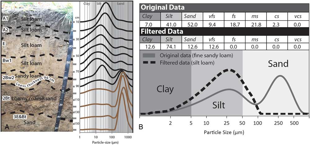
Thin loess deposits are part of a continuum from thicker loess deposits to deposits so thin and intermixed with the underlying sediment as to be initially unrecognizable (Yaalon and Ganor, Reference Yaalon and Ganor1973; Muhs, Reference Muhs, Bettis, Roberts, Harlan, Paces and Reynolds2013a; Luehmann et al., Reference Luehmann, Peter, Connallon, Schaetzl, Smidt, Liu, Kincare, Walkowiak, Thorlund and Holler2016). Therefore, in the past, many such thin loess deposits went unrecognized or misinterpreted. Although much research on thin loess deposits has been focused in the east-central United States (Rutledge et al., Reference Rutledge, Holowaychuk, Hall and Wilding1975; Carey et al., Reference Carey, Cunningham and Williams1976; Foss et al., Reference Foss, Fanning, Miller and Wagner1978; Schaetzl and Loope, Reference Schaetzl and Loope2008; Stanley and Schaetzl, Reference Stanley and Schaetzl2011; Jacobs et al., Reference Jacobs, Mason and Hanson2012; Luehmann et al., Reference Luehmann, Schaetzl, Miller and Bigsby2013, Reference Luehmann, Peter, Connallon, Schaetzl, Smidt, Liu, Kincare, Walkowiak, Thorlund and Holler2016; Schaetzl and Attig, Reference Schaetzl and Attig2013), thin loess deposits occur worldwide (e.g., Litaor, Reference Litaor1987; Hesse and McTainsh, Reference Hesse and McTainsh2003; Muhs and Benedict, 2006; Greene et al., Reference Greene, Cattle and McPherson2009; Lehmkuhl et al., Reference Lehmkuhl, Schulte, Zhao, Hülle, Protze and Stauch2014; Gild et al., Reference Gild, Geitner and Sanders2017; Waroszewski et al., Reference Waroszewski, Sprafke, Kabala, Musztyfaga, Labaz and Woźniczka2017).
Most commonly, thin loess deposits represent the end member of a loess sheet/deposit that is much thicker nearer to its primary source area. The thinning patterns of many loess sheets are well known and can be predicted using statistical models (Fehrenbacher et al., Reference Fehrenbacher, White, Ulrich and Odell1965; Frazee et al., Reference Frazee, Fehrenbacher and Krumbein1970; Kleiss, Reference Kleiss1973; Ruhe, Reference Ruhe1973). By recognizing thin loess deposits as the distal “end members” of thicker loess deposits, the thinning and fining trends of loess may be more accurately described and analyzed. Some thin loess deposits, on the other hand, represent locally sourced sediment that has no association with a “thick end member” (Schaetzl, Reference Schaetzl2008; Luehmann et al., Reference Luehmann, Schaetzl, Miller and Bigsby2013). Source regions for such loess deposits may have been short lived, small in areal extent, or simply low overall dust producers.
For many, the identification of thin loess deposits has proved to be problematic. Normally, the silty textures and pale colors help to identify loess, where present in thick deposits. However, thinner loess is often intermixed with the underlying sediment, sometimes making a clear assessment based on texture ambiguous (Schaetzl and Weisenborn, Reference Schaetzl and Weisenborn2004; Schaetzl, Reference Schaetzl2008; Nyland et al., Reference Nyland, Schaetzl, Ignatov and Miller2017). Methods used to identify loess in thin deposits include (1) changes in texture, often from fine-grained, usually silty, textures in the loess to different textures below (these changes are easiest to interpret where the lithologic contact and texture changes are sharp, and especially where the underlying sediment contains coarse fragments); (2) the presence of quartz or illite (mica) in soils/sediments that have otherwise formed on quartz- and mica-free rocks such as basalt (e.g., Rex et al., Reference Rex, Syers, Jackson and Clayton1969); (3) different values of quartz oxygen isotope ratios or Ti/Zr ratios between the loess and the underlying substrate; and (4) distinct and regular changes in loess particle size across the landscape (Hesse and McTanish, 2003; Muhs, Reference Muhs2013a). Usually, for methods 1–3, data are plotted as depth functions in order to note changes in one or more of these properties with depth (Allan and Hole, Reference Allan and Hole1968; Carey et al., Reference Carey, Cunningham and Williams1976).
Although most loess deposits are originally silt dominated, various postdepositional processes have, in some locations, modified their textural character. For this reason, they have often been misinterpreted, or simply not recognized as loess, thereby requiring inventive methods for their discernment (e.g., Scheib et al., Reference Scheib, Birke and Dinelli2013). Examples from soils in Michigan, USA, illustrate this phenomenon. Here, thin loess commonly overlies sandy sediment. Postdepositional pedoturbation (mixing) has modified the original loess textures—that is, sand from below has been mixed into the loess, resulting in coarse-loamy textures (Schaetzl and Hook, Reference Schaetzl and Hook2008; Schaetzl and Luehmann, Reference Schaetzl and Luehmann2013). Alternatively, sandy sediments in the lower part of the loess deposit may have been locally sourced (i.e., deposited via saltation); this process may have occurred synchronously with early stages of loess deposition, when much of the landscape was not yet loess covered or fully vegetated. Either scenario can result in loess deposits that are sandier than is typical, especially at depth (Schaetzl and Luehmann, Reference Schaetzl and Luehmann2013; Luehmann et al., Reference Luehmann, Peter, Connallon, Schaetzl, Smidt, Liu, Kincare, Walkowiak, Thorlund and Holler2016; Fig. 23A), hindering their recognition in the field. Such “compromised” loess often has distinctly bimodal particle-size curves (Fig. 23B). Ongoing research has shown that, in many areas, soils not known for having loess parent materials actually do have silty surface horizons, or if they have coarse-textured lower profiles, then the upper profile is loamy. Many of these soils have been impacted by thin loess contributions, but until recently, this type of depositional history was not recognized (Munroe et al., Reference Munroe, Attwood, O’Keefe and Quackenbush2015).
Because many thin loess deposits have been texturally altered by postdepositional mixing or by additions of other (coarser) eolian sediment during the loess deposition period (Schaetzl and Luehmann, Reference Schaetzl and Luehmann2013), using texture data from thin loess deposits to examine possible source areas or paleowind-flow patterns can be problematic. For this reason, Luehmann et al. (Reference Luehmann, Schaetzl, Miller and Bigsby2013) developed a textural “filtering” operation that works in most spreadsheet software packages. The filtering method removes the sand data from bimodal particle-size texture curve and recalculates the remaining particle-size data to better reflect the character of the original loess (Fig. 23B). The filtering method has been successfully used in studies of thin loess in midcontinent United States (Schaetzl and Attig, Reference Schaetzl and Attig2013; Luehmann et al., Reference Luehmann, Peter, Connallon, Schaetzl, Smidt, Liu, Kincare, Walkowiak, Thorlund and Holler2016; Nyland et al., Reference Nyland, Schaetzl, Ignatov and Miller2017) and awaits further application and refinement elsewhere.
Most thick loess deposits are the focus of scientists who study paleoenvironments, eolian systems, or stratigraphy. Alternatively, thin loess deposits commonly fall within the realm of soil specialists, many of whom also have an interest in eolian systems. The intellectual draw of thin loess deposits to the soil science community is to be expected: soil development is dramatically affected by even small additions of loess (Simonson, Reference Simonson1995). Small additions of loess to a preexisting soil often have notable impacts on the soil’s texture, hydrology, erodibility, and fertility. Soils formed in thin loess deposits are affected not only by the combination of the two sediment types, but also by the hydrologic impacts of the lithologic contact itself, across which soil permeability values change markedly. Loess is commonly finer than the underlying sediment, which causes wetting fronts to “hang” at the contact zone for some time, leading potentially to increased duration times for saturated conditions, and heightened weathering. This effect can also preferentially cause deposition of illuvial substances at the lithologic contact (Schaetzl, Reference Schaetzl1998) and can reduce the rate at which weathering by-products in the overlying loess are removed from the soil. Thus, some soils formed in thin loess develop heightened concentrations of soluble substances in the overlying loess (Wilding et al., Reference Wilding, Odell, Fehrenbacher and Beavers1963; Indorante, Reference Indorante1998). If the loess overlies a paleosol, these impacts may be even more dramatic.
In sum, thin loess deposits, much more widespread and important than previously thought, are gaining attention worldwide by pedologists, geologists, and eolian scientists. They have great potential to inform the scientific community about paleowind patterns, and knowledge of thin loess additions in soils can help explain many pedogenic characteristics.
From cover sand to loess systems: a continuous spectrum
By Jef Vandenberghe
Periglacial eolian sands
Sedimentary facies, origin, and transport processes:
Eolian sands form in periglacial environments with different facies and morphology, from in situ to reworked deposits and composing sheet or dune forms. They extend over a vast belt in North Europe from northern France to northern Russia (Koster, Reference Koster1988; Kasse, Reference Kasse1997, Reference Kasse2002; Vandenberghe and Kasse, Reference Vandenberghe and Kasse2008), but patchy deposits are also reported in England (Catt, Reference Catt1977; Bateman, Reference Bateman1998), North America (Lea, Reference Lea1990; Lea and Waythomas, Reference Lea and Waythomas1990), and southwestern France (Sitzia et al., Reference Sitzia, Bertran, Bahain, Bateman, Hernandez, Garon and de Lafontaine2015; Bertran et al., Reference Bertran, Liard, Sitzia and Tissoux2016). Their periglacial origin has been evidenced since the pioneering work of Edelman and Crommelin (Reference Edelman and Crommelin1939) and Van der Hammen et al. (Reference Van der Hammen, Maarleveld, Vogel and Zagwijn1967). Because of their variegated nature, this section discusses the different kinds of cover sand deposits, focusing on their facies, depositional systems, environmental conditions, and chronological evolution, and especially their relations with loess deposits. Because of this diversity, periglacial eolian sands have to be categorized. The discussion that follows examines the different categories.
Typical “(primary) cover sands” (Fig. 24A) are characterized by a specific, very finely horizontal-parallel laminated structure. These sands were deposited as a “cover” bed, preserving the preexisting topography, hence their name. As demonstrated by mineralogical analyses, they have been homogenized by saltation over distances on the order of tens of kilometers (Vandenberghe and Krook, Reference Vandenberghe and Krook1981, Reference Vandenberghe and Krook1985). As a result, their grain size is surprisingly constant (around 150 µm modal size) over wide surfaces, independent of the underlying substrate.
(color online) (A) Characteristic horizontal parallel laminated cover sand in the type region of Lutterzand (eastern Netherlands); vertical extent of image is 100 cm. (B) Fluvio-eolian sands consisting of alternating beds of medium-coarse sands, fine sands, and silty fine sands interrupted by phases of nondeposition during which frost cracks could form (e.g., indicated by arrows; eastern Netherlands). Length of trowel is 15 cm. (C) Typical cross-laminated and high-angle bedded sand in a dune of Younger Dryas age (Bosscherheide, Netherlands); activation surfaces are indicated by arrows. Length of spade is 50 cm.

“Reworked (secondary) cover sands” (Fig. 24B) originate from primary cover sand by postdepositional runoff or/and fluvial processes. This reworking has resulted in sedimentary structures typical of flowing water (e.g., channel and ripple cross lamination, thin concave-upward lenses of coarse-grained sand), sheetwash (e.g., parallel strata), and even shallow pools of standing water (e.g., clay or silt drapes, humic beds) (Ruegg, Reference Ruegg1983; Koster, Reference Koster1988). However, because this transport is limited to relatively short distances (tens or hundreds of meters), the deposits have largely maintained the mineralogical and granulometric composition of the source cover sand. This mixed genesis, also described for present-day periglacial environments (Good and Bryant, Reference Good and Bryant1985), is at the origin of their respective designation as “fluvio-eolian” or even “lacustro-eolian” sediments (Vandenberghe and Van Huissteden, Reference Vandenberghe and Van Huissteden1988; Van Huissteden et al., Reference Van Huissteden, Vandenberghe, Van der Hammen and Laan2000), analogous to similar loess deposits (Vandenberghe, Reference Vandenberghe2013; Vandenberghe et al., Reference Vandenberghe, Sun, Wang, Abels and Liu2018).
“Periglacial dune sands” (Fig. 24C) are characterized by their well-expressed dune morphology, some up to a few tens of meters in relief. Their sedimentary structure consists of (low- to high-angle) cross bedding, (sub)horizontal lamination, and occasionally homogeneous beds. Transport was by saltation or in low-suspension clouds (De Ploey, Reference De Ploey1977) over short distances (tens or hundreds of meters). In contrast to the cover sands, these sands have a variable granulometric and mineralogical composition because of their local provenance.
Evolution, age, and environmental conditions of European periglacial eolian sands:
In contrast to loess, periglacial eolian sands mostly date to the last full glacial period in Europe (Weichselian pleniglacial period, ca. 62–14.7 ka, ~Marine Oxygen Isotope Stages [MISs] 4–2). Nonetheless, there do exist some rare, Early Pleistocene cover sand deposits (Kasse, Reference Kasse1993).
During the Weichselian Early and Middle Pleniglacial (ca.62–30 ka, ~MISs 3–4), reworked eolian sands were dominant (Van Huissteden, Reference Van Huissteden1990). This system is consistent with the generally humid conditions during that period, which favored reworking by water on top of a mostly frozen substrate (Böse, Reference Böse1991; Kasse, Reference Kasse1999). The reworking also involved mixing with loess. This system of deposition persisted until ca. 17 ka, although the silt component gradually decreased over time. Sometimes the primary eolian sands were interbedded with water-laid sediments during dry climatic phases or/and in dry topographic positions (Vandenberghe, Reference Vandenberghe1985; Gozdzik, Reference Gozdzik1991). Similar processes of dominant reworking, occasionally interrupted by pure eolian activity, before 17 ka have also been documented in adjacent loess regions (Mücher and Vreeken, Reference Mücher and Vreeken1981; Huijzer, Reference Huijzer1993; Meszner et al., Reference Meszner, Kreutzer, Fuchs and Faust2014; Lehmkuhl et al., Reference Lehmkuhl, Zens, Krauß, Schulte and Kels2016).
At the end of the last glacial period (after 17 ka), postdating the last permafrost maximum, the “typical” (primary) cover sands were deposited across the entire North European cover sand belt (Ruegg, Reference Ruegg1983; Vandenberghe, Reference Vandenberghe1985, Reference Vandenberghe1991; Schwan, Reference Schwan1988; Kasse, Reference Kasse2002; Kasse et al. Reference Kasse, Vandenberghe, De Corte and Van den Haute2007). This period of pure eolian activity was fostered by increased aridity with reduced vegetation cover, attributed to (apart from drier climatic conditions) the disappearance of permafrost that allowed for increased infiltration (Kasse, Reference Kasse1997). This important eolian phase started with widespread deflation, resulting in the formation of a characteristic desert pavement (“Beuningen Gravel Bed”; Van der Hammen et al., Reference Van der Hammen, Maarleveld, Vogel and Zagwijn1967). This prominent (litho-)stratigraphic marker horizon occurs from northern France to northeastern Europe (e.g., Zagwijn and Paepe, Reference Zagwijn and Paepe1968; Lautridou and Sommé, Reference Lautridou and Sommé1981). It was dated by luminescence techniques from the type sections in the eastern Netherlands at 17–15 ka (Bateman and Van Huissteden, Reference Bateman and Van Huissteden1999; Vandenberghe et al., Reference Vandenberghe, Derese, Kasse and Van den haute2013), confirmed both in the Netherlands (Kasse et al., Reference Kasse, Vandenberghe, De Corte and Van den Haute2007) and Belgium (Buylaert et al., Reference Buylaert, Ghysels, Murray, Thomsen, Vandenberghe, De Corte, Heyse and Van den haute2009).
Finally, during the late glacial period (14.7–11.9 ka) dune formation was most prominent, although cover sand deposition may have locally continued (Kasse, Reference Kasse1999). Especially during the Older and Younger Dryas, dunes expanded considerably in north-central Europe (e.g., Nowaczyk, Reference Nowaczyk1986; Bohncke et al., Reference Bohncke, Kasse and Vandenberghe1995; Zeeberg, Reference Zeeberg1998), and during the very dry end of the Younger Dryas (10.5–10.1 ka) in North Europe (e.g., Vandenberghe, 1983; Bohncke et al., Reference Bohncke, Vandenberghe and Huijzer1993). Dunes formed especially along valley margins where sand supplied from (braided) floodplains was captured by the vegetation on the adjacent higher dry areas (Vandenberghe, 1983, Reference Vandenberghe1991). In poorly vegetated areas, dune formation continued into the early Holocene (Kozarski, Reference Kozarski1990; Schwan, Reference Schwan1991; Manikowska, Reference Manikowska1994).
The transitional zone between loess and cover sand
Macroscopically, there is often a sharp spatial boundary between areas of late pleniglacial cover sands and loess areas. However, loess adjacent to the cover sand belt shows distinct transitional properties (e.g., in average grain-size distribution). One example occurs in central Flanders (called the “sandloess belt” by Paepe and Sommé, Reference Paepe and Sommé1970), at the northern fringe of the Central Loess Plateau (e.g., Liu, Reference Liu1985; Nugteren and Vandenberghe, Reference Nugteren and Vandenberghe2004), and in southwestern France (Bertran et al., Reference Bertran, Bateman, Hernandez, Mercier, Millet, Sitzia and Tastet2011). Texturally, the transitional sandloess here is distinctly bimodal, with a fine cover sand grain size (~150 µm) and a typical silt-loess mode (~40 µm). This double composition reflects transport both by saltation and in suspension. Possible source regions of both cover sand and loess (possibly the vast Nordic proglacial areas, floodplains, or large river deltas) and wind directions (varying from north to southwest) are still under discussion (e.g., Lautridou et al., Reference Lautridou, Sommé and Jamagne1984; Schwan, Reference Schwan1988; Renssen et al., Reference Renssen, Kasse, Vandenberghe and Lorenz2007; Schatz et al., Reference Schatz, Qi, Siebel, Wu and Zöller2015). The spatial distribution of the sandloess facies illustrates the downwind transition from cover sand to sandloess to loess, roughly north-northwest to south-southeast both in western Europe (Renssen et al., Reference Renssen, Kasse, Vandenberghe and Lorenz2007) and in northern China (Nugteren and Vandenberghe, Reference Nugteren and Vandenberghe2004). Further, it appears that in the southern Netherlands and Flanders this sandloess occurred more to the north (in proximal position) before the Beuningen desert pavement formed than after (i.e., the cover sand belt advanced distally after that episode; Vandenberghe and Krook, Reference Vandenberghe and Krook1985).
The periglacial loess depositional system
Generally, three modes of primary loess deposition, each with specific grain-size distributions, may be distinguished (Bagnold, Reference Bagnold1941; Pye, Reference Pye1995; Vandenberghe, Reference Vandenberghe2013). Fine sandy deposits are principally transported by saltation (type 1a in Vandenberghe, Reference Vandenberghe2013), whereas two finer-grained populations are transported in suspension (types 1b–c).
Loess type 1b (mainly medium-to-coarse silt [25 to 65 μm]) is transported in short-term, near-surface to low-suspension clouds (Tsoar and Pye, Reference Tsoar and Pye1987) probably during cyclonal dust storm outbreaks and especially under cold conditions (Prins et al., Reference Prins, Vriend, Nugteren, Vandenberghe, Lu, Zheng and Weltje2007). Grain sizes of 35–40 μm are common worldwide in primary loess (e.g., in central and eastern Europe: Bokhorst et al., Reference Bokhorst, Vandenberghe, Sümegi, Lanczont, Gerasimenko, Matviishina, Markovic and Frechen2011; Novothny et al., Reference Novothny, Frechen, Horváth, Wacha and Rolf2011; Vandenberghe et al., Reference Vandenberghe, Markovic, Jovanovic and Hambach2014b; in China: Prins et al., Reference Prins, Vriend, Nugteren, Vandenberghe, Lu, Zheng and Weltje2007, Vriend et al., Reference Vriend, Prins, Buylaert, Vandenberghe and Lu2011, Ijmker et al., Reference Ijmker, Stauch, Dietze, Hartmann, Diekmann, Lockot, Opitz, Wünnemann and Lehmkuhl2012; Dietze et al., Reference Dietze, Wünnemann, Hartmann, Diekmann, Jin, Stauch, Yang and Lehmkuhl2013; Nottebaum et al., Reference Nottebaum, Stauch, Hartmann, Zhang and Lehmkuhl2015; in North America: Muhs and Bettis, Reference Muhs and Bettis2003). However, this grain size may vary slightly according to differing wind energy, and thus transport capacity, which can be influenced by the local topography and surface conditions, including vegetation cover (Schaetzl and Attig, Reference Schaetzl and Attig2013; Vandenberghe, Reference Vandenberghe2013). The sandloess type from the transitional zone (see previous discussion) may be considered as a mixture of loess types 1a and 1b.
Loess type 1c is a fine (clayey) silt with modal diameters between 4 and 22 μm. It has been interpreted as background dust transported in high-suspension clouds over long distances (Zhang et al., Reference Zhang, Arimoto and An1999; Prins et al., Reference Prins, Vriend, Nugteren, Vandenberghe, Lu, Zheng and Weltje2007; Vriend et al., Reference Vriend, Prins, Buylaert, Vandenberghe and Lu2011) and incorporated in the high-level westerlies (Pye and Zhou, Reference Pye and Zhou1989; Pye, Reference Pye1995; Sun et al., Reference Sun, Bloemendal, Rea, Vandenberghe, Jiang, An and Su2002); compare the “small dust” (Stuut et al., Reference Stuut, Smalley and O’Hara-Dhand2009) and the very fine dust transported from central Asia. This dust type is deposited mostly in combination with the coarser-grained silt fraction 1b. It is deposited continuously over time, but it is best expressed in relatively warm conditions when cyclonic dust storms are relatively weak (Vandenberghe et al., Reference Vandenberghe, Renssen, van Huissteden, Nugteren, Konert, Lu, Dodonov and Buylaert2006; Prins et al., Reference Prins, Vriend, Nugteren, Vandenberghe, Lu, Zheng and Weltje2007; Vriend et al., Reference Vriend, Prins, Buylaert, Vandenberghe and Lu2011).
Loess and past cultures
By Piotr Owczarek and Ian Smalley
Changes to farming and stock keeping, along with other measures of development of past cultures, were crucial to the growth and rapid expansion of human groups (Dani and Masson, Reference Dani and Masson1992; Simmons, Reference Simmons2011). The agrarian Neolithic societies in Europe and the rich ancient proto-urban and urban civilization in Asia developed under favorable environmental conditions created by access to water and fertile loess soils. The appearance of early man in China and the development of the Chinese culture have long been associated with loess (Andersson, Reference Andersson1934; Clark and Pigott, Reference Clark and Pigott1965; Watson, Reference Watson1966). The traditional view, as expressed by these scholars, indicates that the distribution of loess corresponds approximately to the areas assigned to the Neolithic tradition of the north, in particular the painted pottery of the Yang-shao people. Ho (Reference Ho1976) demarcated loess regions as the “Cradle of the East” and has clearly demonstrated the links between loess and the Chinese Neolithic. This loess-based Chinese society is the only one of the great ancient civilizations to have survived to the present day. Roxby (Reference Roxby1938) was perhaps the first to link the societal development specifically to loess, and his ideas were developed by Smalley (Reference Smalley1968). Smalley postulated unreasonable amounts of glaciation as a precursor to loess deposit formation, but recent studies have shown that loess material originated in High Asia and its deposition was much influenced by the Yellow River (Stevens et al., Reference Stevens, Adamiec, Bird and Lu2013a). The formation mechanisms for the Chinese loess and the links to early societies now seem to be firmly established.
Central Asia, regarded by many authors as one of the classic loess provinces (Dodonov, Reference Dodonov2007), includes different loess deposits extending from the marginal zones of Taklamakan desert, valleys and piedmont of the Pamir-Alay and Tian Shan mountains, to the southeastern coast of the Caspian Sea (Dodonov, Reference Dodonov1991; Dodonov and Zhou, Reference Dodonov and Zhou2008) (Fig. 25). These areas played a key role in the development of the first agricultural civilizations in this part of Asia. The earliest known remains of production-based economy in central Asia date to the sixth millennium BC (Sarianidi, Reference Sarianidi1992). Early agricultural sites here are known from the area between the Pamir forelands, the upper Amu Darya (Oxus) River, and southern margin of the Karakum desert. These settlements developed on loess patches, as did the First Persian Empire (Achaemenid Empire), and in the next millennia Parthia, Khwarezm, Sogdiana, and Bactria (Dani and Masson, Reference Dani and Masson1992). In the past, more humid climatic conditions occurred in these modern semidesert or desert landscapes (Yang et al., Reference Yang, Wang, Bräuning, Dong and Esper2009; Chen et al., Reference Chen, Chen, Holmes, Boomer, Austin, Gates, Wang, Brooks and Zhang2010). The rise and fall of societies inhabiting central Asia coincided with these climatic fluctuations (Yin et al., Reference Yin, Su and Fang2016).
(color online) Map of loess and loesslike deposits in Asia, with the locations of the most important towns and Silk Road branches on the background of the main kingdoms and empires of the second to third centuries AD. After Dodonov (Reference Dodonov2007), Dodonov and Zhou (Reference Dodonov and Zhou2008), and Owczarek et al. (Reference Owczarek, Opała-Owczarek, Rahmonov, Razzokov, Jary and Niedźwiedź2017).

The first Neolithic cultures also appeared in areas of loess in Europe. Clark (Reference Clark1952) produced an interesting map suggesting the relationship of the settlement of central Europe by Neolithic Danubian peasants to locations of loess deposits. He placed Neolithic sites on a base map of the Grahmann (Reference Grahmann1932) loess map of Europe and showed impressive correlations. Neolithic and earlier Bronze Age settlement systems on the central European uplands and Carpathian forelands also correspond strongly with areas of loess (Kruk et al., Reference Kruk, Alexadrowicz, Milisauskas and Śnieszko1996; Kruk and Milisauskas, Reference Kruk and Milisauskas1999). The spread of the Neolithic to central Europe, between the sixth and fourth millennium BC (Gronenborn, Reference Gronenborn2010), took place along fertile loess uplands occurring on the northern Sudetes and Carpathians forelands.
Loess deposits are interconnected along the course of the Silk Route (Fig. 25), whose peak of influence occurred during the Tang dynasty, in the second part of the first millennium AD (Liu, Reference Liu2010). From Chang’an (Xi’an) in the Chinese Empire, through the rich ancient kingdoms of Loulan, Khotan, Sogdiana, and Khwarezm to the coast of the Caspian Sea, the route clearly coincided with loess areas, where many agricultural settlements occurred. The development of a network of towns and settlements along the Silk Road during this period was possible thanks to fertile loess soils and abundant water (oases, rivers) (Dani and Masson, Reference Dani and Masson1992; Abazow, Reference Abazow2008; Owczarek et al., Reference Owczarek, Opała-Owczarek, Rahmonov, Razzokov, Jary and Niedźwiedź2017). Climate change during the last two millennia, along with human impacts such as deforestation and intensive agriculture, influenced the rise and fall and, in some cases, even the emergence of new settlements in this area, especially in the western piedmont of Pamir and Tian Shan mountains in the Sogdiana (Marshak, Reference Marshak2003). An example of the close relationship between favorable environmental conditions and climate change may be the ancient cities of Niya, Loulan, and Panjikent. Niya and Loulan, centers of the rich Khotan and Loulan kingdoms, were located on the southern and eastern edge of the Taklamakan desert (Yong and Sun, Reference Yong and Sun1994). Both of the cities were developed on the basis of irrigation of loess soils on the terraces of the Niya and Tarim Rivers. Increases in precipitation at ca. 2.1–1.9 ka, noted in the Tarim basin (Wünnemann et al., Reference Wünnemann, Mischke and Chen2006; Chen et al., Reference Chen, Chen, Holmes, Boomer, Austin, Gates, Wang, Brooks and Zhang2010), led to the rapid political and economic development of this area. These rich cities lost their importance after the second century AD, because of long-term drought and shifting and drying of river channels and lakes, and were completely abandoned by the early fifth century (Yong and Sun, Reference Yong and Sun1994). As these kingdoms located on the edge of the Taklamakan desert in the Tarim basin declined, the Sogdiana in western central Asia grew. The Sogdian settlement network, like those of Samarqand and Bukhara, developed on loess patches in the piedmont of Pamir-Alay along the Zarafshan River. One of the towns erected along the Silk Road in the fifth century was Panjikent, which by the end of the seventh century was the most important urban settlement in this part of central Asia (Grenet and de la Vaissière, Reference Grenet and de la Vaissière2002; Marshak, Reference Marshak2003). The city was founded on the upper, loess-mantled terrace of the Zarafshan River (Owczarek et al., Reference Owczarek, Opała-Owczarek, Rahmonov, Razzokov, Jary and Niedźwiedź2017). The ancient town was abandoned in the ninth and tenth centuries. The fall of Panjikent was associated with a political crisis connected to Arab conquest in AD 722 (Grenet and de la Vaissière, Reference Grenet and de la Vaissière2002), during a shift to a drier climate in the eighth to ninth centuries, and an accompanying decline in natural and agricultural resources because of human impacts and erosion of its loess soils (Owczarek et al., Reference Owczarek, Opała-Owczarek, Rahmonov, Razzokov, Jary and Niedźwiedź2017).
The cultural and economic development of human societies is strongly affected by environmental resources. Areas with fertile soil and access to water, characteristics common to most areas of loess, have been shown throughout history to be predisposed for a “Neolithic revolution,” which became a later impulse for the development of modern societies.
Loess geochronology
By Helen M. Roberts
Loess deposits often provide impressive paleoclimatic and paleoenvironmental records. Accurate geochronological data play a critical role in understanding these important terrestrial archives. A number of approaches have been used to establish the timing of events preserved within the loess record, including relative dating techniques and methods to establish age equivalence, as well as radiometric dating techniques to establish numerical ages. The purpose of this section is to consider these different geochronological approaches and their contribution to the study of loess and comment on the likely future research directions for loess geochronology.
The striking visible changes between alternating intercalated loess and paleosol units that can be seen in many loess exposures attests directly to the rhythm of changing climatic conditions through time. This stratigraphy offers a simple relative chronology back through time, across glacial-interglacial cycles, solely based on appearance. If assumptions are made about continuous accumulation rates and preservation of the loess deposits over time, then simple top-down layer counting of the loess-paleosol units can be used to establish the likely ages of the individual units, which in turn allows correlation to other loess sequences on the basis of likely age equivalence, and correlation to other dust-bearing deposits such as terrestrial lake deposits, marine sediments, and ice cores. Correlations of all kinds are dramatically strengthened where isochronous stratigraphic markers preserved in the deposits (e.g., a geochemically distinct tephra) can be identified and used to establish age equivalence; this is especially key for loess deposits. Where the age of these distinctive markers is already known from records elsewhere, this is particularly valuable—for example, the widespread Campanian Ignimbrite/Y5 tephra, dated to ~40 ka, is a key chronostratigraphic marker across the Mediterranean and southeastern Europe (Veres et al., Reference Veres, Lane, Timar-Gabor, Hambach, Constantin, Szakács, Fülling and Onac2013).
Records of paleomagnetic reversals and geomagnetic excursions because of changes in the earth’s geomagnetic field have also played an important role in linking long terrestrial loess sequences to each other and enabling correlation to other long records such as the marine record of Lisiecki and Raymo (Reference Lisiecki and Raymo2005). However, the delay between the deposition of sediment and the immobilization of the magnetic signal results in the apparent downward displacement of the paleomagnetic signature preserved in different records (Zhou and Shackleton, Reference Zhou and Shackleton1999; Sun et al., Reference Sun, Qiang, Liu, Bloemendal and Wang2013; Zhao et al., Reference Zhao, Qiang and Sun2014). This “lock-in effect” requires careful consideration or potentially much higher-resolution sampling (Maher, Reference Maher2016), if high-precision magnetostratigraphy is to be used to link sites with greater temporal precision and accuracy.
Beyond this broad framework of tie points offered through stratigraphy, opportunistic tephra correlation, and magnetostratigraphy, further detail and opportunities for correlation between these indirectly dated records can be provided by fluctuations in records of magnetic susceptibility, grain size, dust flux, and the degree of amino-acid racemization in land snails, which are used to establish age equivalence on the basis of the pattern of their signatures within loess and paleosol units. Magnetic susceptibility and grain-size fluctuations in particular have been widely used for correlation between loess records on the basis of “wiggle matching” (e.g., Yang and Ding, Reference Yang and Ding2014; Marković, this issue); they are often interpreted as climate-related signatures, insomuch as climate cycles largely drive silt generation and loess depositional systems. In some cases, a chronology is established by linking these records to other nonloess records for which more detailed chronological information may have already been established, such as records from lacustrine, marine and ice cores, and speleothems (e.g., Bloemendal et al., Reference Bloemendal, Liu and Rolph1995; Porter and An, Reference Porter and An1995; Vandenberghe et al., Reference Vandenberghe, An, Nugteren, Lu and Van Huissteden1997; Yang and Ding, Reference Yang and Ding2014); in other cases, these records are directly tuned to orbital cycles (Ding et al., Reference Ding, Ranov, Yang, Finaev, Han and Wang2002b; Sun et al, Reference Sun, Clemens, An and Yu2006).
Where only a broad chronostratigraphic framework or methods to establish age equivalence are used, or where proxy records of climate are tuned to orbital frequencies, it is necessary to assume that (1) loess accumulation rates were essentially continuous over time, with no major hiatuses or erosional events, and (2) the rates were constant between chronological tie points. However, these assumptions are being increasingly recognized as an oversimplification of the nature of many loess records, as large (i.e., order of magnitude) fluctuations in accumulation rates have been reported within (Roberts et al., Reference Roberts, Muhs, Wintle, Duller and Bettis2003; Muhs et al., Reference Muhs, Bettis, Roberts, Harlan, Paces and Reynolds2013a; Stevens et al., Reference Stevens, Buylaert, Lu, Thiel, Murray, Frechen, Yi and Zeng2016), as well as between, loess units (Sun and An, Reference Sun and An2005). Additionally, significant hiatuses have been identified (Lu et al., Reference Lu, Stevens, Yi and Sun2006; Terhorst et al., Reference Terhorst, Thiel, Peticzka, Sprafke, Frechen, Fladerer, Roetzel and Neugebauer-Maresch2011). Additionally, indirect dating methods and/or tuning of proxy records to a climate driver, such as orbital cycles, has other potential problems: (1) it involves assumptions about the nature and timing of the records or proxies being investigated, (2) it brings the potential for circular reasoning, and (3) it precludes the opportunity to investigate leads and lags between proxy records of climate change. In contrast, independent numerical dating using radiometric techniques allows loess-paleosol sequences to be linked unambiguously to each other, and to other records with accurate, independent numerical chronologies. This approach allows proxy records and their correlations to be explored within and between sites, rather than being assumed to have the same meaning, timing, and significance at each site. For example, a comparison of several Chinese loess sections with independent radiometric age control (Dong et al., Reference Dong, Wu, Li, Huang and Wen2015) revealed the time-transgressive nature across the sites of rapid changes in the magnetic susceptibility signal inferred to represent the Pleistocene/Holocene transition. The sites spanned a climatic gradient across the Chinese Loess Plateau, and the age for the inferred Pleistocene/Holocene transition was asynchronous across the sites, varying by ~3–4 ka along the northwest (drier, less weathered) to southeast (wetter, more weathered) transect. Furthermore, none of these independently derived numerical ages were synchronous with the age of the Marine Oxygen Isotope Stage 2/1 boundary that would otherwise have been assumed for the Pleistocene/Holocene transition at each site, had there been no independent radiometric chronology to support the magnetic susceptibility data (Dong et al., Reference Dong, Wu, Li, Huang and Wen2015). This example emphasizes the importance of independent numerical dating, where possible.
The key radiometric dating techniques that have helped establish numerical chronologies for loess-paleosol sequences are (1) radiocarbon dating and (2) luminescence dating. Since the earliest application to loess-paleosol sequences, radiocarbon dating has benefited from advances in methods of analysis, improvements in instrumentation, and extensions and refinements to the radiocarbon calibration curve (e.g., Hajdas, Reference Hajdas2008). The radiocarbon method relies on finding suitable, sufficient, in situ organic material for dating and has therefore been particularly applied to paleosols and snail shells in loess deposits (Pigati et al., Reference Pigati, McGeehin, Muhs and Bettis2013; Wang et al., Reference Wang, Zhao, Dong, Zhou, Liu and Zhang2014), although other organic materials such as calcareous earthworm granules have also been used (Moine et al., Reference Moine, Antoine, Hatté, Landais, Mathieu, Prud’homme and Rousseau2017). One key issue regarding the use of radiocarbon techniques for dating loess deposits is the relatively low maximum age that can be achieved, compared with the temporally extensive nature of many loess records. Luminescence dating techniques extend beyond the upper age limit of radiocarbon dating and have played an increasingly significant role in deciphering the chronology of loess-paleosol sequences, as both the accuracy and precision of techniques have improved over time.
Luminescence dating exploits the steady buildup of a time-dependent signal acquired during burial of mineral grains of quartz and feldspar. The event being dated is the last exposure to sunlight during transport, prior to deposition and burial. Luminescence techniques are therefore highly appropriate for application to loess sequences, as the fine-grained nature of this eolian sediment implies long-transport distances, and hence ample time for bleaching of any preexisting luminescence signal prior to deposition; additionally, the method dates the deposition event directly. The method does not typically suffer from lack of suitable materials for dating, being applied to mineral grains of quartz and feldspar, which are abundant in loess and available throughout the sedimentary sequence. One important parameter that does need to be considered though is water content over the depositional period, as water in the pore spaces between grains absorbs radiation that would otherwise reach the sediment grains. Careful assessment must be made as the final luminescence age calculated can change by a little over 1% per 1% change in water content. A combination of local knowledge of water history at the site and measurements of the lower and upper limits of water content are therefore used to define a suitable average value for the water content over the depositional history of the sediments (see also Nelson and Rittenour, Reference Nelson and Rittenour2015).
Today, a family of luminescence techniques exists, and the range of signals available for dating continues to expand. The optically stimulated luminescence (OSL) signal from quartz grains, measured using a single-aliquot regenerative dose protocol, remains the luminescence signal of choice for dating where conditions are appropriate (see review by Roberts, Reference Roberts2008). Unfortunately, the annual dose rate in loess is relatively high, and hence the maximum age limit for quartz OSL is typically significantly less than 100 ka (Chapot et al., Reference Chapot, Roberts, Duller and Lai2012). In contrast, infrared-stimulated luminescence (IRSL) signals from feldspar have a greater saturation dose and hence a greater potential upper age limit. In the past, however, the widespread use of feldspars for dating was impeded by the phenomenon of anomalous fading, leading to age underestimations. A resurgence of interest in the use of feldspars for dating has recently occurred, driven by the discovery of more stable “post-IR IRSL” signals with minimal rates of anomalous fading (see reviews by Buylaert et al., Reference Buylaert, Jain, Murray, Thomsen, Thiel and Sohbati2012; Li and Li, Reference Li and Li2012). Feldspars offer a higher upper age limit of several hundreds of thousand years in loess. Ongoing and future luminescence work relevant to loess studies will likely focus on the development of techniques to reliably extend the upper limit of dating even further. Examples include the infrared photon-luminescence signal from feldspars, which appears not to suffer from anomalous fading (Prasad et al., Reference Prasad, Poolton, Kook and Jain2017); the use of the thermally transferred OSL signal from quartz (Wang et al., Reference Wang, Lu and Wintle2006); and the violet-stimulated luminescence signal, which has been used by Ankjærgaard et al. (Reference Ankjærgaard, Guralinik, Buylaert, Reimann, Yi and Wallinga2016) to significantly extend the age range from quartz by an order of magnitude to ~600 ka in loess.
Aided by the expansion of the range of radiometric techniques available, and an increasingly large number of ages generated, future work within the area of loess geochronology will likely focus on investigating the validity of previous assumptions regarding the steady accumulation rates and quasi-continuous nature of loess accumulation. Future research can address questions relating to the degree of continuity of thick loess records and explore the existence and durations of major hiatuses in the loess sedimentary record. The increased use of independent radiometric dating will also permit further investigation of the degree of (a)synchrony of the proxy records preserved across networks of loess-paleosol sequences, and cross correlations to other long sedimentary records such as marine and ice-core records. This work will, however, necessitate an increasingly dense sampling strategy for radiometric dating, in order to capture the detail required to address these questions. An increased density of independent numerical age determinations will also enable the application of Bayesian statistics to such data sets, giving rise to age-depth models that will further increase the accuracy and precision of loess-paleosol chronologies.
Zircon U-Pb and single-grain provenance techniques in loess research
By Thomas Stevens
Knowledge of loess sources provides information on past dust sources and production, allows proper interpretation of climate proxies, and can yield insights into landscape evolution (Smalley et al., Reference Smalley, O’Hara-Dhand, Wint, Machalett, Jary and Jefferson2009; Nie et al., Reference Nie, Stevens, Rittner, Stockli, Garzanti, Limonta and Bird2015). However, substantial debates still exist over the dust sources of many of the world’s loess deposits (Aleinikoff et al., Reference Aleinikoff, Muhs, Bettis, Johnson, Fanning and Benton2008; Crouvi et al., Reference Crouvi, Amit, Enzel, Porat and Sandler2008; Újvári et al., Reference Újvári, Varga, Ramos, Kovács, Németh and Stevens2012; Stevens et al., Reference Stevens, Carter, Watson, Vermeesch, Andò, Bird, Lu, Garzanti, Cottam and Sevastjanova2013b). Because of the dominance of silt-size particles and the well-known distance-sorting properties of eolian systems, bulk sediment techniques have traditionally been used to address these debates (Chen et al., Reference Chen, Li, Yang, Rao, Lu, Balsam, Sun and Ji2007; Buggle et al., Reference Buggle, Glaser, Zöller, Hambach, Marković, Glaser and Gerasimenko2008). Although they provide valuable information on the fine silt/clay sources and overall compositional characteristics of loess, bulk sediment analyses average out provenance signatures, which may mask specific provenance data if the loess was derived from multiple sources (Stevens et al., Reference Stevens, Palk, Carter, Lu and Clift2010).
In order to circumvent such problems, there has been a surge in use of single-grain techniques to identify loess sources (Aleinikoff et al., Reference Aleinikoff, Muhs, Saner and Fanning1999, Reference Aleinikoff, Muhs, Bettis, Johnson, Fanning and Benton2008; Stevens et al., Reference Stevens, Palk, Carter, Lu and Clift2010; Újvári et al., Reference Újvári, Varga, Ramos, Kovács, Németh and Stevens2012). To date, most such studies have focused on U-Pb ages of multiple individual zircon grains (ZrSiO4). Zircons are heavy minerals (4.65 g/cm) that are resistant to weathering and act as geochemically closed systems through most surface and crustal processes. They crystallize at high temperatures from silica-rich melts and at high grades of metamorphism, with Pb and U retained up to ~900°C. They are nearly ubiquitous in upper crustal rocks and as an accessory mineral in detrital sediments (Hawkesworth and Kemp, Reference Hawkesworth and Kemp2006). Zircons reject radiogenic Pb during their formation, which means that the ages of individual grains, isolated from bulk samples via density and magnetic separation, can be constrained using U-Pb isotopic analysis, often measured using laser ablation inductively coupled mass spectrometry or secondary ion mass spectrometry (Fedo et al., Reference Fedo, Sircombe and Rainbird2003). Zircon U-Pb ages can be highly diagnostic of sediment source, because of the variety of distinct formation ages of their protosource terranes, and the often characteristic zircon U-Pb age distributions in different detrital sediments and rocks. As such, the technique is one of the most widely used provenance methods (Fedo et al., Reference Fedo, Sircombe and Rainbird2003), and zircon U-Pb age data are abundant for many loess potential source areas.
Provenance assignment is undertaken via comparisons of zircon U-Pb age assemblages in target loess sediments to zircon U-Pb data in potential source areas. This comparison is usually based on some graphical form of probability density estimation—for example, a probability density function or kernel density estimator diagram (Fig. 26)—but also potentially via mixture modeling or other statistical approaches. The identification of discrete peaks of specific zircon U-Pb ages or age ranges in a sample facilitates the identification or exclusion of possible sources based on the presence of zircons of these ages in potential source rock samples. A specific example from China is shown in Figure 26, and described subsequently. Because preparation and analysis of samples is relatively time consuming, sampling is often undertaken at rather coarse intervals (meters to tens of meters scale) within a loess section. To ensure sufficient yield of zircons, it is advisable to take ≈1 kg of loess material per sample at the cleaned section. After extraction, grains are usually imaged (often using cathodoluminescence) to check for damage, zonation, and so forth, and to set up targets for analyses. Analyses numbers vary greatly between studies (discussed subsequently), but at a minimum, it is generally accepted that >110 zircon ages are needed to utilize age peak presence as a provenance indicator (Vermeesch, Reference Vermeesch2004), whereas to analyze the absence of ages or the relative heights of peaks generally requires substantially more data (Pullen et al., Reference Pullen, Ibáñez-Mejia, Gehrels, Ibáñez-Mejia and Pecha2014).
(color online) Kernel density estimator diagrams (Vermeesch, Reference Vermeesch2012) of compiled zircon U-Pb age data from studies of the Chinese Loess Plateau. Compiled from Fenn et al. (Reference Fenn, Stevens, Bird, Limonta, Rittner, Vermeesch and Andò2017; see paper for sources). “Chinese Loess Plateau” includes all data from the plateau combined, whereas “loess” and “paleosol” are combined data for Chinese Loess Plateau loess and soil units, respectively. Yellow River (U) refers to the upper river reaches (Nie et al., Reference Nie, Stevens, Rittner, Stockli, Garzanti, Limonta and Bird2015); Mu Us (E) and (W) refer to data from eastern and western parts of the desert, respectively (Stevens et al., Reference Stevens, Carter, Watson, Vermeesch, Andò, Bird, Lu, Garzanti, Cottam and Sevastjanova2013b).

Significant zircon U-Pb data sets exist from both North American (Aleinikoff et al., Reference Aleinikoff, Muhs, Saner and Fanning1999, Reference Aleinikoff, Muhs, Bettis, Johnson, Fanning and Benton2008) and European (Újvári et al., Reference Újvári, Varga, Ramos, Kovács, Németh and Stevens2012) loess, although the majority of data are from Chinese Loess Plateau deposits (Stevens et al., Reference Stevens, Palk, Carter, Lu and Clift2010, Reference Stevens, Carter, Watson, Vermeesch, Andò, Bird, Lu, Garzanti, Cottam and Sevastjanova2013b; Pullen et al., Reference Pullen, Kapp, McCallister, Chang, Gehrels, Garzione, Heermance and Ding2011; Xiao et al., Reference Xiao, Zong, Li, Hu, Dupont-Nivet, Peng and Zhang2012; Che and Li, Reference Che and Li2013; Licht et al., Reference Licht, Pullen, Kapp, Abell and Gieser2016; Fenn et al., Reference Fenn, Stevens, Bird, Limonta, Rittner, Vermeesch and Andò2017). Debate about the origin/provenance of Chinese loess has been rather polarized, with multiple potential source areas, some being thousands of kilometers apart. Chinese Loess Plateau zircon U-Pb age distributions exhibit a distinctive “double peak” of ages of around 260–290 Ma and 440–460 Ma; these ages comprise 80–90% of the zircon grains (Fig. 26). Small numbers of grains have ages of 700–1100 Ma and 1700–2000 Ma. The protosources of these zircon grains must be crystalline/high-grade metamorphic rocks formed at those times, with prime candidates being northern Tibetan Plateau and Gobi Altay mountain terranes (Stevens et al., Reference Stevens, Palk, Carter, Lu and Clift2010). These age peaks can be compared to data obtained from potential source sediments, as they may be indicative of the most recent sediment transport step. Nie et al. (Reference Nie, Stevens, Rittner, Stockli, Garzanti, Limonta and Bird2015) proposed that the Yellow River system was the source for Chinese Loess Plateau deposits, as it transported eroded northeastern Tibetan Plateau sediment (Fig. 26) that is readily available for deflation and eolian transport to the Chinese Loess Plateau. This major revision of prevailing ideas implies that the summer monsoon controls incision of the Tibetan Plateau and may be responsible for the accelerated rates of loess deposition on the plateau, post–3.6 Ma. A number of further U-Pb studies have tested these conclusions (Bird et al., Reference Bird, Stevens, Rittner, Vermeesch, Carter, Andò and Garzanti2015; Licht et al., Reference Licht, Pullen, Kapp, Abell and Gieser2016; Zhang et al., Reference Zhang, Lu, Xu, Liu, Yang, Stevens and Bird2016; Fenn et al., Reference Fenn, Stevens, Bird, Limonta, Rittner, Vermeesch and Andò2017). Licht et al. (Reference Licht, Pullen, Kapp, Abell and Gieser2016) argued that although many potential Chinese loess source areas yield similar zircon age peaks, deriving large data sets (n=400–1000 grains per sample) permits differences in peak proportions to be used to differentiate these source areas. As such, they grouped age data together into loess, paleosol, and potential source area groups and applied mixture-modeling techniques; their work supports the idea that the Yellow River system is indeed the dominant sediment source to the Chinese Loess Plateau (Fig. 26). Licht et al. (Reference Licht, Pullen, Kapp, Abell and Gieser2016) further argued that sediments from the northern Tibetan Plateau Qaidam basin also contributed an equal proportion of sediment to both loess and paleosol units (Fig. 26). As different dust storm tracks likely existed between glacial and interglacial phases, this similar source assemblage implies that predeposited glacial loess material was eroded during interglacial periods and contributed to accretion of soil units, in a process of internal reworking or “eolian cannibalism” (Licht et al., Reference Licht, Pullen, Kapp, Abell and Gieser2016).
A key challenge is to extend these comprehensive analyses to Pliocene red clay deposits that underlie the loess. Although some red clay zircon U-Pb studies have been published (Nie et al., Reference Nie, Song, Möller, Stockli, Peng, Stevens, Bird, Oalmann, Liu, Horton and Fang2014; Shang et al., Reference Shang, Beets, Tang, Prins, Lahaye, van Elsas, Sukselainen and Kaakinen2016; Gong et al., Reference Gong, Xie, Zhang and Zhang2017), the necessary preparation and analysis of smaller zircon grains in the red clays make this work difficult. A further challenge is that the large sample numbers in recent studies require improved analysis and visualization of the resultant data sets. One method to address this is multidimensional scaling (MDS; Vermeesch, Reference Vermeesch2013). MDS constructs a two-dimensional map of individual points that represents samples with multiple analyses numbers; distances on the map indicate the degree of similarity among points (cf. Stevens et al., Reference Stevens, Adamiec, Bird and Lu2013a). Such dimensional reduction techniques are likely to become more important with the increasing importance of “big data” (an Internet-era term used by Vermeesch and Garzanti [Reference Vermeesch and Garzanti2015] to describe the large and complex multisample, multimethod data sets now being generated in many provenance studies). Big data sets also open up the potential for quantification of source contributions from zircon U-Pb data; this is a major topic of interest, with a number of recent approaches proposed (Stevens et al., Reference Stevens, Palk, Carter, Lu and Clift2010; Licht et al., Reference Licht, Pullen, Kapp, Abell and Gieser2016; Zhang et al., Reference Zhang, Lu, Xu, Liu, Yang, Stevens and Bird2016). However, a note of caution has also recently been sounded by Fenn et al. (Reference Fenn, Stevens, Bird, Limonta, Rittner, Vermeesch and Andò2017), who demonstrated that grouping of sample data together can result in spurious trends. Clearly, high analysis numbers and statistical representativity are important, although the number of analyses required depends on the complexity of source assemblages and the specific property of U-Pb age distributions being examined (Vermeesch, Reference Vermeesch2004; Pullen et al., Reference Pullen, Ibáñez-Mejia, Gehrels, Ibáñez-Mejia and Pecha2014). Nonetheless, the goal should be larger numbers of analyses from individual samples, with caution exercised in grouping sample data sets (Fenn et al., Reference Fenn, Stevens, Bird, Limonta, Rittner, Vermeesch and Andò2017).
Zircon U-Pb data are not without limitations—for example, (1) the effect of sedimentary recycling through multiple phases is hard to diagnose; (2) zircon sources may not always be representative of those of the main sediment body; (3) as zircon is a heavy mineral, zircon U-Pb ages will likely reflect more proximal sources; and (4) zircon fertility in source rocks exerts a key control over detrital zircon assemblages (Sláma and Košla, Reference Sláma and Košla2012). As such, a major goal of future research should be to introduce other single-grain analyses that complement zircon U-Pb age analyses. Some initial attempts at this have been made in Chinese loess, combining zircon U-Pb dating with zircon fission-track and heavy mineral analysis (Stevens et al., Reference Stevens, Adamiec, Bird and Lu2013a; Nie et al., Reference Nie, Song, Möller, Stockli, Peng, Stevens, Bird, Oalmann, Liu, Horton and Fang2014, Reference Nie, Stevens, Rittner, Stockli, Garzanti, Limonta and Bird2015) and with garnet chemistry (Fenn et al., Reference Fenn, Stevens, Bird, Limonta, Rittner, Vermeesch and Andò2017). In central-eastern European loess deposits, attempts have been made to combine zircon U-Pb dating with both geochemistry of rutile (Újvári et al., Reference Újvári, Klötzli, Kiraly and Ntaflos2013) and zircon Hf isotopes (Újvári and Klötzli, Reference Újvári and Klötzli2015), as well as bulk geochemical indicators (Újvári et al., Reference Újvári, Varga, Ramos, Kovács, Németh and Stevens2012). Zircon U-Pb analyses have also been combined with Pb isotope analysis of isolated aliquots of K-feldspars in loess in the United States (Aleinikoff et al., Reference Aleinikoff, Muhs, Saner and Fanning1999, Reference Aleinikoff, Muhs, Bettis, Johnson, Fanning and Benton2008). Garnet type and rutile trace element composition in particular have great potential to complement zircon U-Pb dating, especially where source terranes show overlapping zircon U-Pb ages but are composed of rocks of varying metamorphic grade and formation temperatures (Újvári et al., Reference Újvári, Klötzli, Kiraly and Ntaflos2013; Fenn et al., Reference Fenn, Stevens, Bird, Limonta, Rittner, Vermeesch and Andò2017).
In sum, single-grain provenance analysis is a rapidly emerging tool in loess research. Although in many loess regions major breakthroughs in constraining loess-dust sources can be made through the straightforward application of detrital zircon U-Pb dating, multitechnique single-grain approaches promise even more accurate and precise dust sourcing for loess deposits globally.
Acknowledgments
We wish to thank the many people who helped to make the Eau Claire LoessFest a success, especially Doug Faulkner, Garry Running, and Kent Syverson of the University of Wisconsin–Eau Claire; John Attig of the Wisconsin Geological and Natural History Survey; and Kristine Gruley and Joseph Mason of the University of Wisconsin–Madison. Chase Kasmerchak of Michigan State University was a key support person for field trip and conference planning. We thank Michigan State University and the University of Wisconsin–Eau Claire for financial and logistical support and acknowledge receipt of grants in support of the LoessFest from INQUA and the National Science Foundation. This special issue was the idea of Nick Lancaster, editor of Quaternary Research. Nick brought in Art Bettis and Randall Schaetzl as guest editors. The authorship order for this introduction is, after the two editors, alphabetical order by last name of the primary authors, and then again in alphabetical order by last name of the secondary authors. The editors also wish to thank the many reviewers of the papers that follow for their constructive input and expertise. We would especially like to thank Dan Muhs and Peter Jacobs for their thorough reviews of the final “assembled” manuscript. Dan Muhs deserves a special commendation for his thorough and insightful comments and suggestions on the sections entitled “Loess in Alaska” and “Geochemical Approaches to the Study of Loess.” We believe that the 19 contributions in this introduction, and the 19 papers in this LoessFest issue proper, nicely represent the diversity of loess research being done today worldwide and exemplify some of the best that this discipline has to offer. Enjoy.