INTRODUCTION
Several studies have indicated significant climatic changes in the Amazonian region during the Holocene. For instance, in lowland Amazonian Ecuador, periods of severe drought caused significant tree mortality between 8700 and 5800 cal yr BP, with more uniform conditions leading to the development of mature forests after 5800 cal yr BP (Weng et al. Reference Weng, Bush and Athens2002). In the Colombian Amazonia, drier early Holocene and wetter late Holocene conditions were reported (Behling and Hooghiemstra Reference Behling and Hooghiemstra2000). Numerous authors have proposed that the dry Holocene period would have caused the replacement of forest by open savannah in several Amazonian areas, which was followed by forest during the late Holocene due to an increase of precipitation (e.g., Bush and Colinvaux Reference Bush and Colinvaux1988; Absy et al. Reference Absy, Cleef, Fournier, Martin, Servant, Sifeddine, Silva, Soubiès, Suguio, Turcq and Van der Hammen1991; Desjardins et al. Reference Desjardins, Filho, Mariotti, Chauvel and Girardin1996; Pessenda et al. Reference Pessenda, Gomes, Aravena, Ribeiro, Boulet and Gouveia1998a, Reference Pessenda, Gouveia, Aravena, Gomes, Boulet and Ribeiro1998b, Reference Pessenda, Gouveia, Gomes, Boulet and Ribeiro1998c, Reference Pessenda, Boulet, Aravena, Rosolen, Gouveia, Ribeiro and Lamotte2001; Behling and Hooghiemstra Reference Behling and Hooghiemstra1998, Reference Behling and Hooghiemstra1999, Reference Behling and Hooghiemstra2000; Freitas et al. Reference Freitas, Pessenda, Aravena, Gouveia, Ribeiro and Boulet2001; Sifeddine et al. Reference Sifeddine, Bertrand, Fournier, Martin, Servant, Soubiès, Suguio and Turcq1994 Reference Sifeddine, Marint, Turcq, Volkmer-Ribeiro, Soubiès, Cordeiro and Suguio2001; Berrio et al. Reference Berrio, Hooghiemstra, Behling and Van der Borg2000; Weng et al. Reference Weng, Bush and Athens2002; Behling Reference Behling2011; Moreira et al. Reference Moreira, Moreira-Turcq, Turcq, Caquineau and Cordeiro2012; Hermanowki et al. 2012).
From 4000–3000 cal yr BP to the present, there was a moderate and progressive increase in arboreal vegetation in the southern Amazon basin, due to the return to more humid climate conditions that were probably similar to those of the the present day (Freitas et al. Reference Freitas, Pessenda, Aravena, Gouveia, Ribeiro and Boulet2001; Pessenda et al. Reference Pessenda, Ribeiro, Gouveia, Aravena, Boulet and Bendassoli2004). Isotopic studies in a southern Amazonian region and on a 1600-km transect covering three states of northeastern Amazonia indicated drier climate during the mid-Holocene and forest expansion associated with a wetter period during the last 3000 years (Pessenda et al. Reference Pessenda, Gomes, Aravena, Ribeiro, Boulet and Gouveia1998a, Reference Pessenda, Gouveia, Aravena, Gomes, Boulet and Ribeiro1998b, Reference Pessenda, Gouveia, Gomes, Boulet and Ribeiro1998c). Others studies have indicated that the climatic conditions in the Amazon Basin were drier during the early and mid-Holocene (e.g. Absy Reference Absy1979; Gouveia et al. Reference Gouveia, Pessenda, Aravena, Boulet, Roveratti and Gomes1997; Behling and Costa Reference Behling and Costa2000; Sifeddine et al. Reference Sifeddine, Bertrand, Fournier, Martin, Servant, Soubiès, Suguio and Turcq1994; Mayle et al. Reference Mayle, Burbridge and Killeen2000; Sifeddine et al. Reference Sifeddine, Marint, Turcq, Volkmer-Ribeiro, Soubiès, Cordeiro and Suguio2001; Cordeiro et al. Reference Cordeiro, Turcq, Turcq, Moreira, Rodrigues, Costa, Sifeddine and Simões Filho2008; Mayle and Power Reference Mayle and Power2008; Hermanowski et al. Reference Hermanowski, Costa, Carvalho and Behling2012) and changed to a wetter climate during the late Holocene (e.g. Behling and Costa Reference Behling and Costa2000; Bush et al. Reference Bush, Silman and Listopad2007; Cordeiro et al. Reference Cordeiro, Turcq, Turcq, Moreira, Rodrigues, Costa, Sifeddine and Simões Filho2008).
There is still a lack of consensus about the Holocene climate, and particularly about the presence of a middle Holocene dry period in the Brazilian Amazonian lowland. For instance, several authors have defended that there is no evidence for a significant climatic change during most of the Holocene (e.g., Behling and Costa Reference Behling and Costa2000; Bush et al. Reference Bush, Miller, de Oliveira and Colinvaux2000; Behling et al. Reference Behling, Cohen and Lara2001; Irion et al. Reference Irion, Bush, Nunes de Mello, Stüben, Neumann, Müller, Morais de and Junk2006; Miranda et al. Reference Miranda, Rossetti and Pessenda2009; Castro et al. Reference Castro, Rossetti and Pessenda2010; Zani et al. Reference Zani, Rossetti, Cohen, Pessenda and Cremon2012). This debate motivated us present this work, which provides pollen and radiocarbon (14C) data of deposits from old fluvial terraces along the Branco River in northeastern Amazonia. These data allow to reconstruct vegetation patterns for the past 5000 cal yr BP and further discuss about the climate that prevailed in this area during this time frame.
STUDY AREA
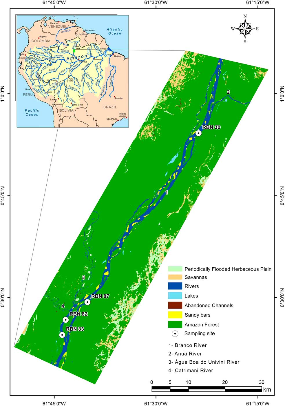
The study area is located along the Branco River in the State of Roraima (Figure 1). The Branco River basin is formed by the junction of the Tacutu and Urariocoera Rivers, about 30 km upstream of the city of Boa Vista. The segment of the Branco River studied here is located approximately 550 km northward of its confluence with the Negro River (Figure 1). This area is inserted in the Pantanal Setentrional Basin, an area of Quaternary sediments (Santos et al. Reference Santos, Nelson and Geovannini1993) mainly formed in megafan depositional systems (Rossetti et al. Reference Rossetti, Zani and Cremon2014), which is bounded to the north, east, and west by Precambrian crystalline rocks of the Guiana Shield. The study area encompasses late Pleistocene to Holocene sands and muds surrounded by alluvial deposits of the Plio-Pleistocene Içá Formation (RADAMBRASIL 1976).
Location of the study area showing the geomorphological features and vegetation units along the Branco River.

A typical tropical climate, with a well-defined dry season and an average annual rainfall between 1700 and 2000 mm/year prevails in the study area. Average annual temperatures range from 26°C to 33°C (RADAMBRASIL 1975). The Intertropical Convergence Zone (ITCZ) and the El Niño/La Niña–Southern Oscillation (ENSO) play important roles on the interannual rainfall regime in this region (Latrubesse and Nelson Reference Latrubesse and Nelson2001).
The State of Roraima has a vegetation cover represented by a mosaic that consists of large areas of open vegetation either intermingled or in sharp contact with the Amazonian rainforest (Serruya Reference Serruya2002; Ab’Saber Reference Ab’Saber1989). The latter show variation in physiognomy and structure according to their environment. The forest vary from várzea, igapó, and hilltop “islands” with terra-firme forest (Gribel 2009; Laranjeiras et al. Reference Laranjeiras, Naka, Bechtoldt, da Costa, Andretti, Cerqueira, de Fátima Torres, Rodrigues, Santos, Vargas, Pacheco, Sardelli, Mazar-Barnett and Cohn-Haft2014). Fluvial plains are dominated by várzea forest mainly represented by Arecaceae (Veloso et al. Reference Veloso, Rangel-Filho and Lima1991). In these lowland areas, trees are relatively thick, with heights between 30 and 40 m near drainages. This vegetation is mainly represented by Annonaceae, Burseraceae, Humiriaceae, Euphorbiaceae, Myrtaceae, Melastomataceae, Apocynaceae, and Vochysiaceae, among others (IBGE 2012). In addition, the study area also contains white-sand forest locally known as campina or campinarana, with various types (i.e., grassland, shrubland, arboreous, or forest campinaranas; Gribel 2009) However, campinaranas are more generally characterized by Poaceae and Cyperaceae, which are surrounded by the rainforest mainly represented by Bombacaceae, Euphorbiaceae, Sapotaceae, Moraceae, Fabaceae, Malpighiaceae, Rubiaceae, Bignoniaceae, Rubiaceae, Melastomataceae, Arecaceae, Mouriri sp., Sacoglottis guianensis, and Caraipa savannarrum (Anderson Reference Anderson1981; Gribel et al. Reference Gribel, Ferreira, Coelho, Santos, Ramos and Silva2009).
MATERIAL AND METHODS
Field Sampling and Sediment Description
In order to obtain a continuous pollen record throughout the Holocene, 10 cores were sampled depths up to 10 m using a Russian sampler. However, only four cores presented suitable pollen concentration to a consistent statistical analysis. Three cores were taken from old fluvial terraces located about 10 m higher than the modern floodplain at the margin of the Branco River (Figure 1), and they were named RBN 30 (0°54′11.9′′N, 61°23′41.8′′W), RBN 82 (0°26′42.7′′N, 61°43′16.1′′W), and RBN 83 (0°24′29.4′′N, 61°43′47.0′′W). One core, RBN 87 (0°29′19.9′′N, 61°40′04.3′′W) was sampled from an abandoned channel (Figure 1). These sampling sites are dominated by dense rainforest.
Facies descriptions included observations of lithology, texture and structure, and they aimed interpretation of depositional environments. These sedimentary characteristics were recorded on a measured lithostratigraphic profile. Grain size for the interval with pollen data was determined in more detail by laser diffraction using a Laser Particle Size SHIMADZU SALD 2101 in the Laboratory of Chemical Oceanography/UFPA. Prior to grain size analysis, approximately 0.5 g of each sample was immersed in H2O2 to remove organic matter, and the residual sediments were disaggregated by ultrasound (França et al. Reference França, Francisquini, Cohen, Pessenda, Rossetti, Guimarães and Smith2012). The grain-size scale of Wentworth (Reference Wentworth1922) was used in this work with sand (2–0.0625 μm), silt (62.5–3.9 μm), and clay fractions (3.9–0.12 μm).
Pollen Analysis
For pollen analysis, 1.0 cm3 of sediment were collected in intervals of 2.5 (RBN 30) and 5 cm (RBN 82, 83, and 87), which totaled 85 samples. All samples were prepared using standard pollen analytical techniques including acetolysis (Faegri and Iversen Reference Faegri and Iversen1989). Sample residues were mounted on slides in glycerin jelly. Pollen and spores were identified by comparison with reference collections of about 4000 Brazilian forest taxa and various pollen keys (Salgado-Labouriau Reference Salgado-Labouriau1973; Absy Reference Absy1975; Markgraf and D’Antoni Reference Markgraf and D’Antoni1978; Roubik and Moreno Reference Roubik and Moreno1991; Colinvaux et al. Reference Colinvaux, De Oliveira and Patiño1999), jointly with the reference collections of the Laboratory of Coastal Dynamics–Federal University of Pará and 14C Laboratory of the Center for Nuclear Energy in Agriculture (CENA/USP) to identify pollen grains and spores. A minimum of 300 pollen grains were usually counted for each sample, but for some specific depths 200 or 250 grains were counted due to their low pollen concentrations. Microfossils consisting of spores, algae, and some fungi were also counted, but they were not included in the sum.
All pollen taxa present were identified, but only the most abundant were plotted in pollen diagrams in order to illustrate the different ecological groups. The pollen diagrams were statistically subdivided into assemblage zones using a square-root transformation of the percentage data, followed by stratigraphically constrained cluster analysis (Grimm Reference Grimm1987). The intervals not analyzed by pollen content along the stratigraphic profiles exhibit absolute absence of pollen.
Radiocarbon Dating
Based on lithostratigraphic changes, seven samples of sedimentary organic matter (10 g each) were selected for 14C analysis, two in each of the cores Rbn82, Rbn83, Rbn30, and one in core Rbn87. Dating was carried out at the BETA Analytic Laboratory and LACUFF (Fluminense Federal University–Brazil) using accelerator mass spectrometers (AMS).
At the BETA Analytic Laboratory, sample pretreatment and dating followed the Beta Analytic for Radiocarbon Dating Laboratory standard technique for accelerator mass spectrometry (AMS) dating. The pretreatment consisted of dispersing the sediment deionized water, followed by sieving through 180-micron sieve to recover any available plant material and to remove any stones, gravel or other course inorganic grains. The less than 180-micron size fraction was used in each case. Two 0.1N HCl baths where applied for 2 hr each at 70ºC to remove any carbonates. Samples were rinsed to neutral and dried at 100ºC for 12 hr, cooled and weighed. After homogenizing with mortar and pestle, a small portion of the sediment was tested under a microscope with 12M HCl to ensure complete removal of all carbonate. Each sample was subsampled and combusted to CO2 in a closed chemistry line which has been purged of any CO2 to a level below 10e–15 atoms (background levels). The CO2 was then introduced into a reaction vessel containing an aliquot of cobalt metal catalyst. Hydrogen was introduced such that when the cocktail was heated to 500ºC, the CO2 cracked to carbon (graphite). The graphite was pressed into a target for measurement in an AMS system. The AMS was calibrated to provide an accurate ratio of the 14C/13C ratio between the sample graphite and a modern reference (NIST–4990C, oxalic acid). Quality assurance (QA) samples were reacted simultaneously in the chemistry lab and measured simultaneously in the AMS. The analytical result was obtained as a fraction of the value of modern reference, corrected for isotopic fractionation using 13C/12C (δ13C) and 14C age calculated according to the conventions cited in Stuiver and Polach (Reference Stuiver and Polach1977). The QA samples were checked for accuracy and observed to fall within expectations for the laboratory to accept and report the sample results. The QA acceptance was defined as the total laboratory error known to be within 2σ. The equipment used in these analyses were the Thermo Delta-Plus isotope ratio mass spectrometer (δ13C precision of ± 0.3‰) and the 250 kV NEC single stage particle accelerator (AMS precision of ±0.001 – 0.004 fractions modern) (http://www.radiocarbon.com/PDF/Beta-AMS-Methodology.pdf).
The samples dated at the LACUFF were previously examined and physically cleaned under a stereomicroscope. The organic matter (humin) from sediment samples were extracted according to the laboratory standard pretreatment with the acid–alkali–acid method (Pessenda et. al. 1996). At LACUFF, the samples were converted to carbon dioxide organic samples and all gas samples were cryogenically purified. Graphitization method and other procedures in the LACUFF laboratory can be obtained in Macario et al. (Reference Macario, Gomes, Anjos, Carvalho, Linares, Alves, Oliveira, Castro, Chanca, Silveira, Pessenda, Moraes, Campos and Cherkinsky2013). Results are expressed as radiocarbon ages (14C yr BP) normalized to a δ13C of –25‰ PDB, presently denoted as VPDB, or percentage of modern carbon (pMC) (Stuiver and Polach Reference Stuiver and Polach1977). 14C ages were also reported as calibrated years [cal yr BP, 2σ using CALIB 7.1 software and SHcal13 curve (Reimer Reference Reimer2013) and CALIBomb (Reimer et al. 2004)].
RESULTS
14C and Sedimentation Rates
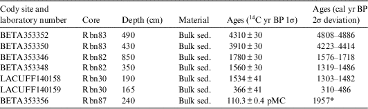
The validity of 14C dates extracted from organic matter in sedimentary environments such as lakes, bogs, and fluvial plains has been evaluated (Turney et al. Reference Turney, Coope, Harkness, Lowe and Walker2000; Lowe et al. Reference Lowe, Walker, Scott, Harkness, Bryant and Davies2004; Howard et al. Reference Howard, Gearey, Hill, Fletcher and Marshall2009), and extensively used to provide robust chronologies for landscape evolution, particularly the timing and correlation of climatic and sea-level-change events (e.g. Pessenda et al. Reference Pessenda, Vidotto, De Oliveira, Buso, Cohen, Rossetti, de Ricardi-Branco and Bendassolli2012; Cohen et al. Reference Cohen, Rossetti, Pessenda, Friaes and Oliveira2014, Reference Cohen, Pessenda, Behling, Rossetti, França, Guimarães, Friaes and Smith2012; Rossetti et al. Reference Rossetti, Polizel, Cohen and Pessenda2015). Howard et al. (Reference Howard, Gearey, Hill, Fletcher and Marshall2009) tested the validity of 14C dating in fluvial sedimentary deposits and the humin and humic acid fraction dating revealed results statistically consistent, where the humin and humic acid fraction provide the more reliable age estimates for each dated sample depth in fluvial sediments. In addition, this study revealed that plant macrofossils produce younger dates than the humic and humin fractions. Regarding our 14C dates, obtained along cores sampled from fluvial plains, these data provide a coherent chronological framework for a lithostratigraphic and pollen analysis (Table 1). No age reversal was recorded. The oldest ages were recorded at the base of the lithostratigraphic profile from where core RBN 83 was acquired. The age of 4808–4886 cal yr BP was obtained from the middle part of this core, and another age of 4223–4414 cal yr BP occurs in the first overlying mud, located only 0.6 m upward. Core RBN 82 was acquired at the top of a lithostratigraphic profile displaying ages of 1576–1718 and 1319–1486 cal yr BP. The pollen profile RBN 30 was dated at the base at 1303–1482 yr BP and at the top as 310–486 cal yr BP. The youngest age was recorded at the base of pollen profile RBN87, revealing a modern 14C content indicative of post-thermonuclear testing era (110.3% ± 0.4 pMC 1957 cal AD), indicating an essentially modern age.
Sediment samples selected for radiocarbon dating with material depth 14C conventional and calibrated ages (using Calib 7.1 and SHcal13 curve, Reimer et al. 2013; and CALIBomb, Reimer et al. 2004).

* Cal AD.
Considering a linear interpolation between age control points, the sedimentation rate in core RBN 82 is 20 mm/yr (850–350 cm). RBN 83 presents rates between 1.13 (490–430 cm) and 0.98 mm/yr (430–0 cm), and RBN 30 core presents rates about 0.25 mm/yr (190–165 cm) and RBN 87 presents 43 mm/yr (240–0 cm). As noted in some studies in the northern Amazon (Behling et al. Reference Behling, Cohen and Lara2004; Cohen et al. Reference Cohen, Behling and Lara2005a, Reference Cohen, Lara, Smith, Angélica, Dias and Pequeno2008, Reference Cohen, Lara, Smith, Matos and Vedel2009; Vedel et al. Reference Vedel, Behling, Cohen and Lara2006; Guimarães et al. Reference Guimarães, Cohen, França, Lara and Behling2010) these differences in sedimentation rates are related to the settling velocity of sediments, since larger diameter particles (e.g. gravel and sand) settle faster than fine particles (e.g. silt and mud), and water velocities necessary to carry large particles in suspension are greater than those needed to keep fine particles suspended.
Sediment Description
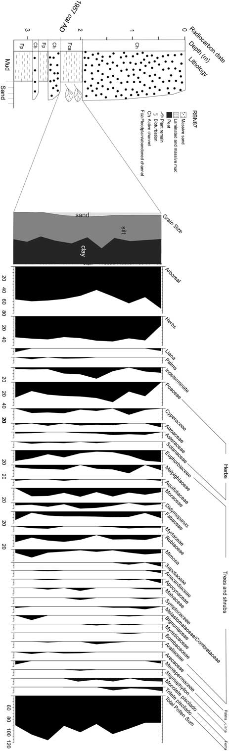
Core RBN 87 was acquired from a succession of circa 3-m-thick sediments, represented muddy deposits interbedded by sands (Figure 2). The latter display sharp, erosional, and concave-up bases, and they grade upward from coarse/medium- to medium/fine- and then fine-grained. These deposits are massive, moderate to well sorted, and mostly composed by quartz grains. The muddy sediments are either massive or parallel-laminated and they vary from light to dark gray in color. Core RBN 87 was obtained between 2.4 and 2 m depth, and consists only of dark gray, parallel-laminated muds with abundant plant remains. Detailed grain size analysis revealed a composition of 45% clay, 50% silt, and 5% sand. These deposits occur in a concave-up morphology, grading downward into massive sands to complete a fining upward succession. Upward, they are sharply overlain by a thicker, i.e., up to 2-m-thick fining upward sandy succession.
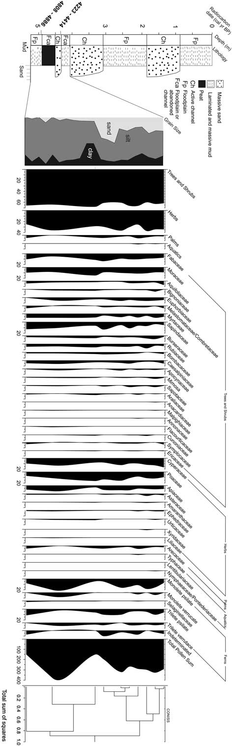
Summarized results for core Rbn-83 with variation as a function of core depth showing chronological and lithological profiles with sedimentary facies as well as ecological pollen groups and percentages of the most frequent pollen taxa zones and cluster analysis.

RBN 83 was acquired from a 5.2-m-thick river bank composed of sands and muds distributed in almost equivalent proportion (Figure 3). The sandy deposits have grain sizes similar to RBN87, they also fine upward, and are based by sharp and erosional and concave-up surfaces. Most of the muds occur outside the concave-up shapes, and they display light gray to greenish colors. Core RBN83 records the lowermost 0.7 cm of this lithostratigraphic profile, being represented by at the base by 0.3 cm thick massive greenish gray mud and 40-cm-thick peat layer at the top. Interesting is that, despite the muddy nature, the contact between these deposits is defined by a sharp and also slightly concave-up discontinuity surface. Detailed grain-size analysis revealed mean values for clay of 25%, silt of 60%, and sand of 15%.
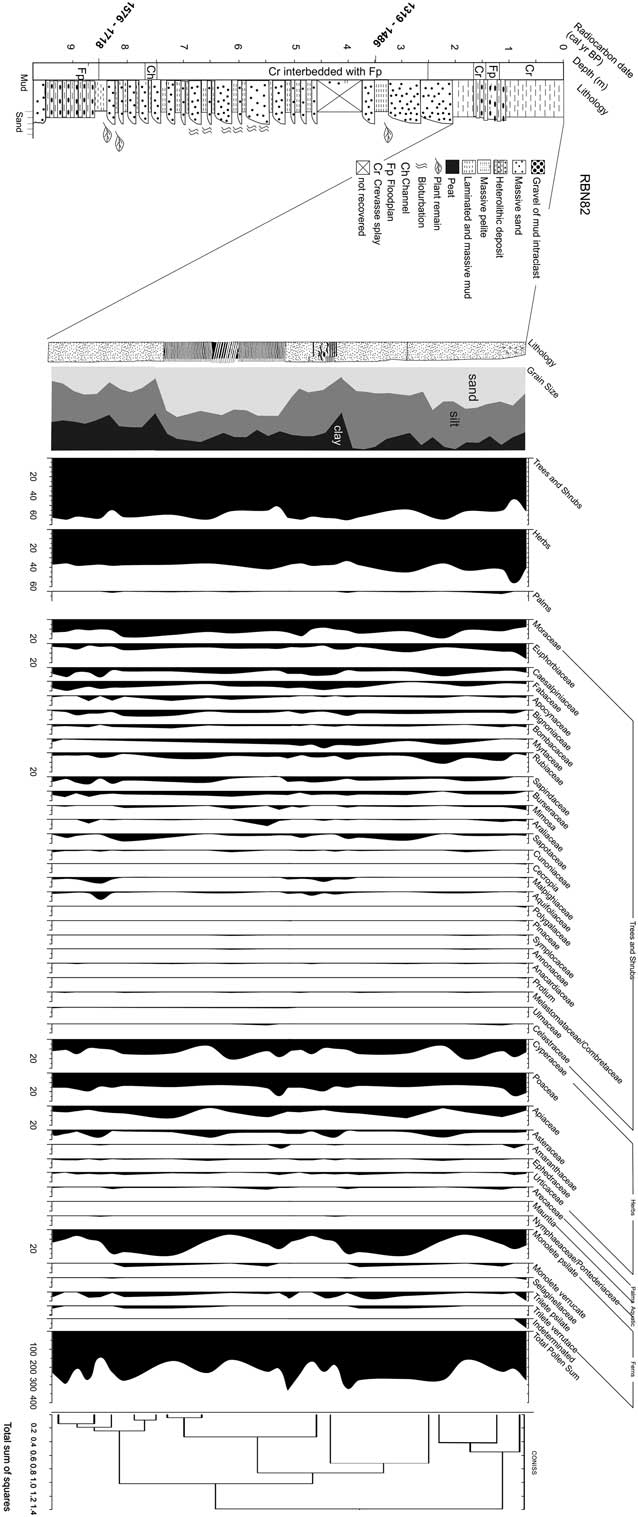
Summarized results for core Rbn-82 with variation as a function of core depth showing chronological and lithological profiles with sedimentary facies as well as ecological pollen groups and percentages of the most frequent pollen taxa zones and cluster analysis.

RBN 82 derives from a 9.7-m-thick sedimentary succession (Figure 4) also consisting of interbedded sands and muds, but which displays a vertical organization completely different from the two previously described profiles. Hence, sand beds are progressively thicker upward, configuring an overall thickening upward succession. In addition, individual sand beds, which are massive or bioturbated and lenticular in shape, grade upward from very fine to fine-, or fine to medium-grained. Downward, they grade into mud layers, completing several coarsening upward successions. As opposed to their gradational basis, the top of the sand beds is essentially sharp. The muds in this profile vary from light to dark gray. They are massive or parallel-laminated and locally they alternate rhythmically with sand laminae to form lenticular heterolithic bedddings. Core RBN82 was acquired at the topo of this succession, where a 2.2-m-thick interval of dark gray organic mud is present. Detailed grain-size analysis revealed mean values of 20% clay 20%, 40% silt, and 40% sand.
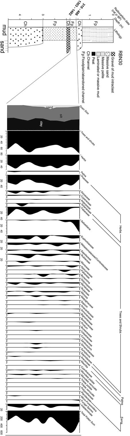
Summarized results for core Rbn-30 with variation as a function of core depth showing chronological and lithological profiles with sedimentary facies as well as ecological pollen groups and percentages of the most frequent pollen taxa.

RBN 30 derives from a 4.5-m-thick sedimentary succession consisting of muds and sands arranged into fining upward cycles (Figure 5). Three of these cycles are present, which were caused by sharp and erosional discontinuity surfaces mantled by coarse-grained sands or gravel with mud intraclasts. Upward, these deposits grade into medium- and then fine-grained sands, or they grade directly into laminated or massive muds, as well as massive pelite. RBN30 was acquired from a 0.6-cm-thick interval consisting of dark-gray, organic muds with parallel lamination that overlie directly a package of gravel with mud intraclast. Detailed grain-size analysis revealed mean values of 40% clay, 55% silt, and 5% sand.
Summarized results for core Rbn-87 with variation as a function of core depth showing chronological and lithological profiles with sedimentary facies as well as ecological pollen groups and percentages of the most frequent pollen taxa.

Pollen Analysis
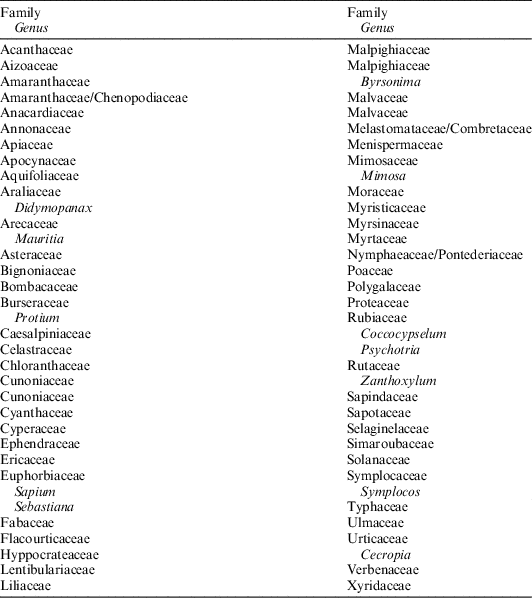
Seventy pollen taxa were identified (Table 2), but the diagrams (Figures 2–5) show only the most abundant taxa (>3% pollen sum) and the different ecological groups. The pollen grains identified in the core RBN83 was accumulated between 4808–4886 and 4223–4414 cal yr BP. Trees and shrubs pollen dominate the pollen assemblage (60–68%), and they are mainly represented by Sapindaceae (7–16%), Fabaceae (5–15%), Moraceae (10–15%), Myrtaceae (5–8%), Rubiaceae (5–8%), Aquifoliaceae (0–7%), Bignoniaceae (0–5%), Euphorbiaceae (1–5%), Melastomataceae/Combretaceae (0–5%), Bombacaceae (0–3%) and Sapotaceae (0–4%), while herb pollen (25–38%) are mainly characterized by Cyperaceae (7–18%), Poaceae (10–17%) and Apiaceae (5–10%) and Asteraceae (0–3%). Arecaceae presents low percentages (0–3%).
Taxa identified in the studied cores.

The pollen content of the RBN30, deposited between 1303–1482 and 310–486 cal yr BP, presents trees and shrubs (45–78%) mainly consisting of Sebastiana (0–43%), Fabaceae (5–25%), Melastomataceae/Combretaceae (5–15%), Euphobiaceae (2–15%), Sapotaceae (0–9%), Rubiaceae (2–15%), Moraceae (0–5%), Apocynaceae (0–6%), Byrsonima (0–10%), Myrtaceae (0–8%), Didymopanax (0–3%), Malpighiacaeae (0–5%). Herb pollen (25–48%) are mostly characterized by Poaceae (16–45%), Aizoaceae (2–10%), Solanaceae (0–10%), and Cyperaceae (0–3%).
Considering the mean sedimentation rates obtained to RBN82, the pollen assemblage analysed was accumulated during the last 1576–1718 cal yr BP. Trees and shrubs (45–65%) dominate the pollen profile, which is mainly represented by Moraceae (8–25%), Euphorbiaceae (3–15%), Caesalpiniaceae (5–10%), Fabaceae (2–10%) Rubiaceae (1–11%), Apocynaceae (0–5%), Bignoniaceae (1–6%), Bombacaceae (0–4%), Sapotaceae (0–9%), Myrtaceae (0–10%), Sapindaceae (0–8%), Burseraceae (0–5%), Araliaceae (0–6%), and Malpighiaceae (0–6%). Herb pollen (35–55%) are mainly evidenced by Poaceae (15–25%), Cyperaceae (10–20%), Apiaceae (2–12%), Asteraceae (1–7%), and Amaranthaceae (0–4%).
The pollen assemblage obtained from core RBN87 was deposited after 1957 cal AD. This pollen profile is dominated by the high abundance of trees and shrubs (40–73%), which are mainly characterized by Euphorbiaceae (2–20%), Moraceae (7–15%), Fabaceae (3–15%), Malpighiaceae (2–15%), Didymopanax (0–10%), Myrtaceae (0–5%), Rubiaceae (0–12%), Sapotaceae (0–6%), Bignoniaceae (0–7%), and Melastomataceae/Combretaceae (0–5%). Herb pollen (16–44%) are mostly represented by Poaceae (2–35%), Mimosa (2–14%), Cyperaceae (2–11%), Aizoaceae (0–7%), and Asteraceae (0–5%).
INTERPRETATION AND DISCUSSION
The lithostratigraphic profiles containing the pollen cores described in this study are dominated by sequences of sandy sediments grading upward into mud deposits. These vertical changes, with grain-size decreases with height above the base, characterize fining upward cycles. This structure is consistent with stratigraphic successions developed according to the local fluvial dynamics. Fluvial deposits commonly consist of fining-upward facies successions (Walker Reference Walker1992). The sharp, erosional, and concave-up bases of individual sandy packages conform with deposition in confined environments, typical of channels. Mud deposits overlying these channels were either formed by mud settling from suspensions in abandoned channels or nearby floodplains. Muds formed overlying concave up sharp discontinuity surfaces, as recorded in RBN83, are probably the record of stagnant conditions within mud plugs or small lakes developed along floodplains.
On the other hand, the several coarsening upward lenses recorded in the lithostratigraphic profile, where core RBN 82 was acquired, records a distinct sedimentary process. In this instance, the upward increase in grain size indicates increasing flow energy through time. Considering deposition in a fluvial system, the occurrence of sandy lenses having this characteristic gradationally overlying muds is more likely attributed to episodic sand inflow within low energy environments dominated by mud deposition from suspensions. Such a situation is commonly verified during flooding, when fluvial channels cannot bear their flows, and discharge into adjacent floodplains, forming crevasse splays. Hence, this lithostratigraphic profile records a succession of crevasse splay deposits formed during progressively increased flooding, with the top muds recorded by the core RBN 82 representing the return to normal conditions, when the floodplain was again dominated by low energy mud settling.
The modern hydrographic basin of the Branco River presents many abandoned channels and oxbow lakes along its floodplain (Figure 1). These geomorphologic features are caused by channel shifting, which results in meander cutoff and channel-belt avulsion (Toonen et al. Reference Toonen, Kleinhans and Cohen2012). They are identified in the study site as depressions of considerable reduced width and depth. These features result from autogenic processes inherent to sedimentary dynamics. They represent depressions that are sediment traps with high preservation potential to pollen grains (Kasse et al. Reference Kasse, Hoek, Bohncke, Konert, Weijers, Cassee and Van der Zee2005; Bos et al. Reference Bos, Dambeck, Kalis, Schweizer and Thiemeyer2008; Cohen et al. Reference Cohen, Rossetti, Pessenda, Friaes and Oliveira2014), as indicated by the analysis of the studied fluvial deposits preserved along the Branco River terraces.
Lakes and floodplains generally provide suitable conditions for mud accumulation and preservation of pollen grains sourced by vegetation from the time that sediment was deposited. Lacustrine sediments preserve pollen sourced from vegetation surrounding the lakes, and the spatial representativeness of the lacustrine pollen signal depends on the winds and the extension of the drainage system. The proportion of the pollen signal provided by each vegetation type is distance-weighted (e.g. Davis Reference Davis2000; Xu et al. Reference Xu, Tian, Bunting, Li, Ding, Cao and He2012). Open vegetation is likely to have a higher proportion of long-distance transport pollen rain, but under a relatively closed canopy the sediment should record a small spatial representation of the nearby vegetation (Weng et al. Reference Weng, Bush and Silman2004b; Gosling et al. Reference Gosling, Mayle, Tate and Killeen2009). Our stratigraphic record during the middle and late Holocene showed predominantly arboreal vegetation, whose pollen were probably accumulated around relatively small body of water of floodplain areas similar to those found today in the study site (Figure 1). Such a condition may have attenuated the eventual effect of wind transport. Thus, the pollen profile should represent the paleovegetation of this drainage basin.
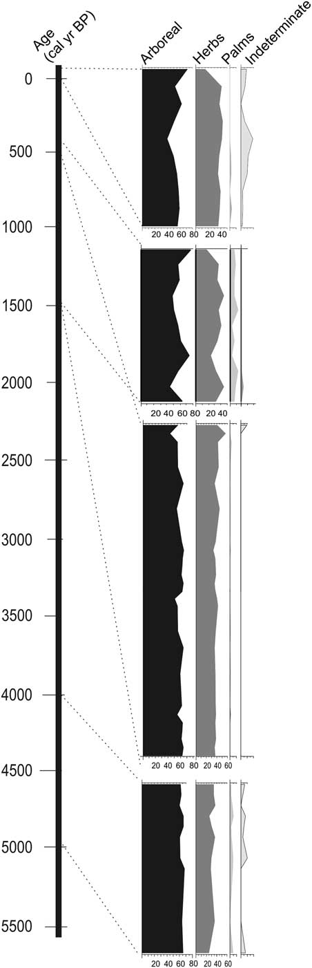
Therefore, the analyzed sediments, accumulated during the middle and late Holocene, indicate a mixture of forest vegetation and herbaceous communities comparable to the local modern vegetation (Figure 6). Considering a dry climatic phase until the middle Holocene, it would cause an expansion of herbaceous in detriment of arboreal vegetation in the study area, producing a significant increase in percentage of herbs pollen grains along the sediments accumulated during the middle Holocene. Such evidence has not been recorded in the core Rbn83 (Figure 2).
Temporal integration of the ecological pollen groups identified in studied cores.

Causes for Vegetation Stability During the Middle and Late Holocene
The modern plant distribution in the Amazonian region has been widely debated, with main hypotheses having considered the influence of climate (ter Steege et al. 2003; Ruter et al. Reference Ruter, Arzt and Vavrus2004), topography (Vormisto et al. Reference Vormisto, Phillips and Ruokolainen2000), soil (ter Steege et al. Reference ter Steege, Jetten and Polak1993), and geology (Räsänen et al. Reference Räsänen, Salo and Kalliola1987; Van der Hammen et al. Reference Van der Hammen, Duivenvoorden, Lips, Urrego and Espejo1992; Zani et al. Reference Zani, Rossetti, Cohen, Pessenda and Cremon2012). In this context, patches of open vegetation that are commonly found intermingled with the Amazonian rainforest have been interpreted as remnants of a vegetation cover formed due to the presence of a dry period during the late Pleistocene (Ledru et al. Reference Ledru, Ceccantini, Gouveia, Lopez–Sáez, Pessenda and Ribeiro2006) and early to middle Holocene (Freitas et al. Reference Freitas, Pessenda, Aravena, Gouveia, Ribeiro and Boulet2001; Pessenda et al. Reference Pessenda, Boulet, Aravena, Rosolen, Gouveia, Ribeiro and Lamotte2001, Reference Pessenda, Ribeiro, Gouveia, Aravena, Boulet and Bendassoli2004).
Some works propose changes in the physical environment as the main factor to the establishment of vegetation patterns in Amazonia through time, as well as other areas around the globe (Van der Hammen et al. Reference Van der Hammen, Duivenvoorden, Lips, Urrego and Espejo1992; Behling and Hooghiemstra Reference Behling and Hooghiemstra2000; Maslin and Burns Reference Maslin and Burns2000; Freitas et al. Reference Freitas, Pessenda, Aravena, Gouveia, Ribeiro and Boulet2001; Sifeddine et al. Reference Sifeddine, Marint, Turcq, Volkmer-Ribeiro, Soubiès, Cordeiro and Suguio2001; Mayle and Power Reference Mayle and Power2008). For instance, the climate changed gradually from dry to wetter after the Last Glacial Maximum (LGM), which appears to have been accompanied by changes in the fluvial discharge (Latrubesse and Ramonell Reference Latrubesse and Ramonell1994; Latrubesse Reference Latrubesse2002; Rigsby et al. Reference Rigsby, Hemric and Baker2009). An increment of up to 40% of humidity after the Younger Dryas was proposed for this region (Maslin and Burns Reference Maslin and Burns2000).
The prevalence of wet conditions since the middle Holocene has been proposed for several areas of the Brazilian Amazonia (Maslin and Burns Reference Maslin and Burns2000; Pessenda et al. Reference Pessenda, Boulet, Aravena, Rosolen, Gouveia, Ribeiro and Lamotte2001; Sifeddine et al. Reference Sifeddine, Marint, Turcq, Volkmer-Ribeiro, Soubiès, Cordeiro and Suguio2001; Rossetti et al. Reference Rossetti, Toledo, Moraes-Santos and Santos2004, Reference Rossetti, Toledo and Góes2005; Jacob et al. Reference Jacob, Huang and Disnar2007; Cordeiro et al. Reference Cordeiro, Turcq, Sifeddine, Lacerda, Silva Filho, Gueiros, Cunha, Santelli, Pádua and Pachinelam2011), which coincided with the expansion of tropical forest as we know it today. The melting of the global ice volume during the transition from the last glacial stage into the current interglacial phase culminated with the global rise in sea level of up to 5 m above the modern sea level in the middle Holocene (Shackleton Reference Shackleton1988), which consequently caused an increase of humidity. Climatic and sea-level changes during the Holocene influenced significantly the development of mangrove along coastal Amazonian areas (e.g., Cohen et al. Reference Cohen, Pessenda, Behling, Rossetti, França, Guimarães, Friaes and Smith2012).
The data presented here indicate a mixture of forest and herbaceous communities comparable to the modern vegetation mosaic of the study area (Figure 6). They also suggest a wet period at least over the last 4808–4886 cal yr BP, without any indication of an expressive vegetation change as a consequence of any eventual middle Holocene dry event.
Some hypotheses may be raised to justify the stability of vegetation patterns in the study site since the middle Holocene. Hence, one possibility is that many Amazonian areas were not under the effect of dry climates during this time frame. In fact, speleothem oxygen isotope indicates that ecosystems in western Amazonia have not experienced prolonged drying over the past 94,000 years (Mosblech et al. Reference Mosblech, Bush, Gosling, Hodell, Thomas, Van Calsteren, Correa-Metrio, Valencia, Curtis and Van Woesik2012). In addition, an integrated approach combining pollen and diatom data from the Marajó Island, located at the mouth of the Amazon River in northeastern Amazonia, recorded no significant change in vegetation during the late Pleistocene through the early/mid Holocene (Castro et al. Reference Castro, Oliveira, Rossetti and Pessenda2013). A drastic middle Holocene change from forest to grassland vegetation was related by these authors to sedimentary influence resulting from coast progradation due to a drop in relative sea-level rather than a drier climate, because these are dominantly C3 herbs typical of wet areas (see also Miranda et al. Reference Miranda, Rossetti and Pessenda2009 and Castro et al. Reference Castro, Rossetti and Pessenda2010). C and N isotope analyses of organic matter from sediments from an area of northern Amazonia located only around 30 km to the east of the study area (Zani et al. Reference Zani, Rossetti, Cohen, Pessenda and Cremon2012) led to state asyncronical development of open vegetation during the middle to late Holocene which was controlled by sedimentary dynamics, rather than climatic changes. In addition, no evidence of mid-Holocene dry climate was found in lakes near Prainha, central Amazonia (Bush et al. Reference Bush, Miller, de Oliveira and Colinvaux2000). Furthermore, a continuous record of forests was documented in the Caxiuaná area, northeastern Amazonia, for the last 7800–7940 cal yr BP (Behling and Costa Reference Behling and Costa2000). Lake Calado, near Manaus, displayed dense tropical forest since 8280–8380 cal yr BP (Behling et al. Reference Behling, Cohen and Lara2001). Several works stated that the Amazonia rainforest was most likely undisturbed during the last 50,000 years (e.g., Colinvaux et al. Reference Colinvaux, De Oliveira, Moreno, Miller and Bush1996, 2001; Bush et al. 2004; Irion et al. Reference Irion, Bush, Nunes de Mello, Stüben, Neumann, Müller, Morais de and Junk2006; Toledo and Bush 2007; Mayle and Power Reference Mayle and Power2008).
Another possibility to consider is that the impact of the dry period, claimed by several authors to have occurred in this region during the early and middle Holocene, did not influence this particular site of the Amazonian forest. It is interestingly to mention that, in contrast to many other Amazonian areas, this particular region currently displays a peculiar climatic regime strongly influenced by the periodic dislocation of the ITCZ. This results from changes in the Atlantic meridional overturning circulation (Chiang and Bitz Reference Chiang and Bitz2005) and/or tropical air–sea interactions, such as the El Niño and La Niña events (Broecker Reference Broecker2003). Therefore, one possibility is that, while a dry climate was in effect in other Amazonian areas, this site may have remained wet at least since the mid-Holocene under influence of the ITCZ dislocation dynamics.
On the other hand, considering the hypothesis of a dry Amazonia during the early and mid-Holocene, then a further hypothesis to be considered is that stabilization of the sea-level about 6000–5000 cal yr BP (Cohen et al. Reference Cohen, Souza Filho, Lara, Behling and Angulo2005b) may have attenuated the climate change, causing no impact on the vegetation cover. Existing RSL curves present dissimilar patterns for the late Holocene in Brazil. The first suggests a RSL fall in the last 5100 yr BP (5647–5999 cal yr BP) with two oscillations (Suguio et al. Reference Suguio, Martin, Bittencourt, Dominguez, Flexor and Azevedo1985a). Angulo and Lessa (Reference Angulo and Lessa1997) and Angulo et al. (Reference Angulo, Giannini, Suguio and Pessenda1999) disagree with the low RSL between 4100–3800 yr BP (~4560– ~4130 cal yr BP) and 3000–2700 yr BP (~3100–~2800 cal yr BP). Tomazelli (Reference Tomazelli1990) suggests a RSL rise in the last 1000 years in the State of Rio Grande do Sul State.
Regarding the northern Brazilian littoral, the RSL stabilized at its current level between ~7000 and ~5000 cal yr BP (e.g., Behling and Costa Reference Behling and Costa2001; Behling et al. Reference Behling, Cohen and Lara2001; Behling Reference Behling2002, Reference Behling2011; Cohen et al. Reference Cohen, Behling and Lara2005b; Souza Filho et al. Reference Souza Filho, Martins and Costa2006; Vedel et al. Reference Vedel, Behling, Cohen and Lara2006). The history of RSL fluctuations on northern Brazilian littoral seems to have been affected by tectonic activity during the late Pleistocene and Holocene (Rossetti et al. Reference Rossetti, Valeriano, Goes and Thales2008, Reference Rossetti, Souza, Prado and Elis2012). The post-glacial sea-level rise, combined with tectonic subsidence, caused a marine transgression during the late Pleistocene and early Holocene along the northern Brazilian coast (Cohen et al. Reference Cohen, Pessenda, Behling, Rossetti, França, Guimarães, Friaes and Smith2012). Between ~5100 and ~1000 cal yr BP, the RSL at the northern Brazil was probably never higher than 0.6 m above the current level (Cohen et al. Reference Cohen, Souza Filho, Lara, Behling and Angulo2005b). A work from the Lago do Crispim in the northeastern State of Pará, which is located next to the present coastline and only 1 m above msl, suggested no flooding during the last ~8800 cal yr BP (Behling and Costa Reference Behling and Costa2001).
At the global scale, sea-level is the dominant driver of the water table depth (Fan et al. Reference Fan, Li and Miguez-Macho2013). Then, sea-level changes during the Holocene might have influenced the shallow groundwater effects on terrestrial ecosystems by sustaining river base-flow and root-zone soil water in the absence of rain (Fan et al. Reference Fan, Li and Miguez-Macho2013). Consequently, regarding a stable relative sea-level along the northern Brazilian littoral during the last 6000 cal yr BP (e.g., Behling et al. Reference Behling, Cohen and Lara2001; Cohen et al. Reference Cohen, Behling and Lara2005b, Reference Cohen, Pessenda, Behling, Rossetti, França, Guimarães, Friaes and Smith2012; Vedel et al. Reference Vedel, Behling, Cohen and Lara2006), the water table depth may have favored the establishment and maintenance of the Amazon lowland forest during the middle and late Holocene. Such event may have created an ecological barrier between a narrow aquatic zone, favoring the development of Amazonian lowland forests at the feet of a large belt of topographic higher hinterlands.
Eustatic sea-level changes since the Pleistocene have caused significant impact on the extent and composition of the Amazonian floodplain. As a consequence of the increased gradient, caused by the decline of ca. 120 m in sea level during the LGM, the rivers cut deeply into their beds and a large volume of sediments were deposited in the Amazon fan (Junk Reference Junk1997). At this time, river valleys became incised, and may have filled with fluvial deposits. Alternatively, the valleys may have remained essentially empty until the next transgression (Walker Reference Walker1992). Geomorphological, sedimentological, and hydrological studies conducted along the Amazonian region upstream and downstream of the Negro River indicate that the várzea (floodplain) reached its present extent after sea-level stabilization, at 5000–6000 cal yr BP ( Irion et al. Reference Irion, Junk and Mello JASN1997; Behling et al. Reference Behling, Arz, Pätzold and Wefer2002). Similar conclusion emerged from detailed examination of riverbed morphologies at the Amazon mouth (Junk Reference Junk1994; Irion et al. Reference Irion, Junk and Mello JASN1997; Vital et al. Reference Vital, Stattegger, Posewang and Theilen1998).
Regarding the present work, in order to obtain a pollen record since the early Holocene, some cores were sampled with depths up to 10 m. However, all 14C dates obtained to the studied deposits indicated mid- and late Holocene. Although this study has not presented a pollen record since the early Holocene, the sediment deposits accumulated since ~4800 cal yr BP, from the base of the core RBN–83, may be an evidence for the time of the flood plain stabilization in a new level along the Branco River. Considering this hypothesis, the sea level rise during the early Holocene and its stabilization at the current level in the northern Brazilian coast, between 6000 and 5000 cal yr BP, may have caused the establishment of a fluvial terrace for accumulation of that sediments since the middle Holocene. Then, the absence of early Holocene sediments in the studied fluvial terrace may be related to the stabilization of the relative sea level in its modern level just in the middle Holocene. Older sedimentary deposits may have been eroded during the relative sea-level rise. Similar process was recorded for the Cardoso Island, São Paulo (Pessenda et al. Reference Pessenda, Vidotto, De Oliveira, Buso, Cohen, Rossetti, de Ricardi-Branco and Bendassolli2012).
Today, the Amazon River and its tributaries are affected by dynamic tides, but without saltwater intrusion due to the high freshwater discharge, as far as 1100 km upstream of its mouth (Kosuth et al. Reference Kosuth, Calléde, Laraque, Filizola, Guyot, Seyler, Fritsch and Guimarães2009; Freitas et al. Reference Freitas, Silva, Souza Filho, Ogston, Nittrouer and Asp2014). On the coastal zone, the stabilization of sea-level allowed development of wetlands (Cohen et al. Reference Cohen, Pessenda, Behling, Rossetti, França, Guimarães, Friaes and Smith2012), while the rainfall inland favored expansion of forest vegetation, the development of perennial streams, and the diversification of terrestrial and aquatic fauna (Meggers Reference Meggers2007).
Therefore, if a dry climate occurred in Amazonia during the Holocene, the most likely is that the stabilization of the relative sea-level since the middle Holocene, may have contributed to the development of the Amazonian lowland forest, having attenuated the impact of the middle Holocene dry period on vegetation in areas under most fluvial influence. In this case, no major vegetation changes are expected after the stabilization of relative sea-level in areas affected by the Amazon drainage system. Studies carried out in the Amazon have shown a buffer effect for areas close to rainforest, where the forest reveals mechanisms of protection against drier periods (Pessenda et al. Reference Pessenda, Valencia, Martinelli and Cerri1996).
CONCLUSIONS
Palynological analyses of fluvial deposits from the Branco River indicate a mixture of forest vegetation and herbaceous communities comparable to the modern one since the mid-Holocene. Then, significant vegetation changes did not occur in the study site during this time interval. The pollen data suggest a wet period similar to the modern one at least over the last 4808–4886 cal yr BP rather than a dry event in the mid-Holocene, as reported for many other Amazonian areas. One possibility is that Amazonia was never under the effect of a dry climate during most of the Holocene. Another hypothesis is that the impact of the dry period occurred during this time did not influence the studied site. On the other hand, taking into account a dry mid-Holocene climate, the stabilization of the relative sea-level, about 6000–5000 cal yr BP along the northern Brazilian littoral, may have affected the water base level along the rivers, and it favored the establishment and maintenance of Amazonian lowland forests even under dry periods. Sea level may have attenuated the impact of dry periods in areas under fluvial influence.
ACKNOWLEDGMENTS
The authors wish to thank the Research Funding Institute of the State of São Paulo (FAPESP–Project #13/50475-5) for the financial support of this research. Brazil’s National Council for Scientific and Technological Development provided research fellowships to the authors. The ICM-Bio-Chico Mendes Institute for Biodiversity Conservation helped with the logistic during the fieldwork.