1 Introduction
A substance which is released into a flowing liquid is subject to advection by the flow and molecular diffusion. The combination of both mechanisms leads to a smearing out of the substance concentration in space and time. Understanding the often complex interplay between these two physically very different effects is important in various situations such as dispersion of pollutants in rivers or the distribution of medical drugs in blood flow.
The governing equation for the time- and space-dependent concentration of the substance in flow is a Fokker–Planck-type convection–diffusion equation which can be formulated by straightforward mass conservation. A full analytical solution, however, does not exist even for the most simple situation of a Poiseuille flow in a straight cylindrical channel with a non-reacting boundary. Extensive studies have therefore focussed on the more tractable long-time regime starting with the pioneering works by Taylor (Reference Taylor1953), Aris (Reference Aris1956) and Chatwin (Reference Chatwin1970). Their central assumption is that the elapsed time since the injection of the substance is long enough that the radial concentration profile is completely uniform. By then considering only radially averaged concentrations, the problem becomes one-dimensional and is amenable to an analytical solution showing that the concentration spreads with an effective diffusion coefficient which is a combination of the molecular diffusion coefficient and the shear dispersion due to the external flow. Over the last decades this so-called Taylor–Aris solution has been extended in various directions including novel derivation and solution methods (Giona & Cerbelli Reference Giona and Cerbelli2010; Berezhkovskii Reference Berezhkovskii2012), non-steady flows (Ng Reference Ng2006; Vedel & Bruus Reference Vedel and Bruus2012), slip effects and elastic boundaries (Ng Reference Ng2010; Daddi-Moussa-Ider, Guckenberger & Gekle Reference Daddi-Moussa-Ider, Guckenberger and Gekle2016; Daddi-Moussa-Ider & Gekle Reference Daddi-Moussa-Ider and Gekle2016; Daddi-Moussa-Ider, Lisicki & Gekle Reference Daddi-Moussa-Ider, Lisicki and Gekle2017), point-like initial release conditions and larger particle sizes (Vedel, Hovad & Bruus Reference Vedel, Hovad and Bruus2014; Howard et al.
Reference Howard, Gautam, Panagiotopoulos and Nikoubashman2016), curved, oscillatory and finite-length channels (Balasubramanian, Jayaraman & Iyengar Reference Balasubramanian, Jayaraman and Iyengar1997; Dorfman Reference Dorfman2009; Giona et al.
Reference Giona, Adrover, Cerbelli and Garofalo2009; Adrover Reference Adrover2011, Reference Adrover2013), additional forces and potentials (Nacev et al.
Reference Nacev, Beni, Bruno and Shapiro2011; Giona & Garofalo Reference Giona and Garofalo2015), ring geometries (Sankarasubramanian & Gill Reference Sankarasubramanian and Gill1971; Ramachandra Rao & Deshikachar Reference Ramachandra Rao and Deshikachar1987; Jayaraman, Pedley & Goyal Reference Jayaraman, Pedley and Goyal1998; Sarkar & Jayaraman Reference Sarkar and Jayaraman2002; Mondal & Mazumder Reference Mondal and Mazumder2005), the inclusion of an adsorbing–desorbing layer on the channel walls (Purnama Reference Purnama1988; Phillips, Kaye & Robinson Reference Phillips, Kaye and Robinson1995; Phillips & Kaye Reference Phillips and Kaye1998; Ng & Rudraiah Reference Ng and Rudraiah2008; Hansen et al.
Reference Hansen, Bruus, Callisen and Hassager2012; Berezhkovskii & Skvortsov Reference Berezhkovskii and Skvortsov2013; Hlushkou et al.
Reference Hlushkou, Gritti, Guiochon, Seidel-Morgenstern and Tallarek2014), substance release from the channel walls (Adrover & Pedacchia Reference Adrover and Pedacchia2013, Reference Adrover and Pedacchia2014), superhydrophobic walls (Bhaumik, Kannan & DasGupta Reference Bhaumik, Kannan and Dasgupta2015) or dead ends (Dagdug, Berezhkovskii & Skvortsov Reference Dagdug, Berezhkovskii and Skvortsov2014). Partially absorbing channel walls have been studied by Sankarasubramanian & Gill (Reference Sankarasubramanian and Gill1973), Davidson & Schroter (Reference Davidson and Schroter1983), Smith (Reference Smith1983), Barton (Reference Barton1984), Mazumder & Das (Reference Mazumder and Das1992), Purnama (Reference Purnama1995), Phillips et al. (Reference Phillips, Kaye and Robinson1995), Balasubramanian et al. (Reference Balasubramanian, Jayaraman and Iyengar1997), Jayaraman et al. (Reference Jayaraman, Pedley and Goyal1998), Sarkar & Jayaraman (Reference Sarkar and Jayaraman2002), Ng (Reference Ng2006), Biswas & Sen (Reference Biswas and Sen2007), Balakotaiah (Reference Balakotaiah2008), Dorfman & Brenner (Reference Dorfman and Brenner2008), Biswas & Sen (Reference Biswas and Sen2008), Ng & Rudraiah (Reference Ng and Rudraiah2008), Mazumder & Paul (Reference Mazumder and Paul2011), Kumar, Umavathi & Basavaraj (Reference Kumar, Umavathi and Basavaraj2012), Dagdug, Berezhkovskii & Skvortsov (Reference Dagdug, Berezhkovskii and Skvortsov2015), Skvortsov, Berezhkovskii & Dagdug (Reference Skvortsov, Berezhkovskii and Dagdug2015) who found that, in general, the radially averaged solute concentration becomes skewed due to absorption on the boundary. As pointed out by Ng & Rudraiah (Reference Ng and Rudraiah2008), however, the Taylor–Aris approach is applicable only in situations where the boundary is weakly absorbing. The reason is fairly obvious: if any substance molecule is immediately absorbed as soon as it touches the boundary, radial homogenization which is the prerequisite for the Taylor–Aris method, becomes impossible. Regarding the initial regime at short times, it has been shown that the width of cross-sectionally averaged distributions shows anomalous diffusion (Lighthill Reference Lighthill1966; Latini & Bernoff Reference Latini and Bernoff2001; Camassa, Lin & McLaughlin Reference Camassa, Lin and McLaughlin2010). Muradoglu, Günther & Stone (Reference Muradoglu, Günther and Stone2007) and Muradoglu (Reference Muradoglu2010) studied solute dispersion between a train of moving bubbles focussing mainly on the exchange of solute between the bubble compartments. All works mentioned in this paragraph have in common that the substance at
 $t=0$
appears instantaneously ‘out of nothing’.
Here, we consider the convection–diffusion problem for a substance which is released instantaneously from the surface of a sphere flowing freely through a cylindrical channel with perfectly absorbing walls. The physical situation that we have in mind is a drug carrier particle which flows through a blood vessel and at a certain point in time releases a pharmaceutical molecule. Once the molecule reaches the cylinder wall it reacts immediately, mimicking absorption of the drug by endothelial cells. The two important quantities are (i) the mean residence time
 $\unicode[STIX]{x1D70F}_{1}$
defined as the time that the molecule spends inside the blood stream before reacting with the boundary and (ii) the width of the axial distribution
 $\unicode[STIX]{x1D70E}_{\unicode[STIX]{x1D701}}$
over which the substance is spread out when it is absorbed on the boundary. The latter is not to be confused with the commonly studied Taylor–Aris-like distribution width inside the flow (taken a at a fixed point in time) since different parts of the substance reach the wall at different times. The width of this reaction position distribution is important to estimate the intensity of the biochemical reaction which will depend on the local concentration.
The situation investigated in this work is qualitatively different from classical Taylor–Aris type of problems as it introduces an internal moving boundary (the sphere) and as the flow field has a small, but non-negligible radial component. As we shall show in this work, these differences lead in general to a reduction of the mean residence time and to a reduction of the width of the reaction position distribution compared to a simple estimate using the Taylor–Aris dispersion coefficient. We furthermore find a strong dependence of
 $\unicode[STIX]{x1D70F}_{1}$
and
 $\unicode[STIX]{x1D70E}_{\unicode[STIX]{x1D701}}$
on the release position. Substance molecules released around the front are quickly dragged away from the sphere and disperse in a very similar manner as a substance released in pure Poiseuille flow. If the substance is released around the tail of the sphere the flow pushes the substance against the sphere leading to reduced residence times similar to the situation between two cylinders. The result is a strongly peaked distribution of the reaction position. At small Péclet numbers
 $\unicode[STIX]{x1D70F}_{1}$
and
 $\unicode[STIX]{x1D70E}_{\unicode[STIX]{x1D701}}$
vary gradually between these two extremes when the release position is moved over the sphere surface. At intermediate and large
 $Pe$
, however, the transition becomes very abrupt causing a well-separated upstream and downstream dispersion regime. The most relevant release position around the equator is always situated in the downstream regime where dispersion is strongly affected by the presence of the sphere.
Finally, we investigate a scenario in which the substance is released continuously from the sphere surface with a prescribed rate.
2 System set-up
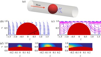
We consider a sphere travelling force free along the centreline of a cylindrical channel as illustrated in figure 1(a). In the following,
 $R$
,
 $\unicode[STIX]{x1D703}$
and
 $\unicode[STIX]{x1D719}$
refer to spherical coordinates while
 $r$
,
 $z$
and
 $\unicode[STIX]{x1D719}$
refer to cylindrical coordinates. At
 $z\rightarrow \pm \infty$
the flow has a Poiseuille profile with the centreline velocity
 $U_{max}$
. In such a situation the flow field
 $\boldsymbol{U}(r,z)$
has been analytically computed by Leichtberg, Pfeffer & Weinbaum (Reference Leichtberg, Pfeffer and Weinbaum1976) and Yeh & Keh (Reference Yeh and Keh2013) as sketched briefly in appendix A and shown in figure 1(b). The sphere is found to travel with a velocity
 $U_{s}$
which satisfies
 $1/2<U_{s}/U_{max}<1$
. Thus,
 $U_{s}$
is larger than the average velocity
 $U_{max}/2$
at
 $z\rightarrow \pm \infty$
and therefore, in the reference frame of the moving sphere, the net flow through the gap between sphere and cylinder is negative as shown in figure 1(c). Furthermore, the upstream flow is separated into two regions: one for which streamlines starting at
 $z\rightarrow \infty$
pass by the sphere towards
 $-\infty$
and one where the streamlines turn around and move back towards
 $+\infty$
. The radial position of this separating streamline depends on the sphere radius and is shown in figure 9 in appendix B.
(a) Illustration of the considered system. (b) Analytical flow field for a sphere with radius
 $R_{s}=0.9$
travelling through a channel as computed by Leichtberg et al. (Reference Leichtberg, Pfeffer and Weinbaum1976) and Yeh & Keh (Reference Yeh and Keh2013). (c) Flow field relative to the moving sphere. The flow through the gap is negative relative to the sphere. (d) Concentration profiles if a unit amount of substance is released at the equator at
 $t=0$
with
 $Pe=100$
, displayed at
 $t=0.0005,0.005,0.0125$
after release.

At time
 $t=0$
a unit amount of substance is released on a ring with constant
 $\unicode[STIX]{x1D703}_{0}$
on the sphere surface. Subsequently, the substance is subject to molecular diffusion and advection by the flow. We only consider the axisymmetric situation where the concentration is averaged over the azimuthal angle
 $\unicode[STIX]{x1D719}$
. The concentration profile
 $c(r,z,t)$
is described by the convection–diffusion (Fokker–Planck) equation. Normalizing as usual all length scales by the cylinder radius
 $r_{c}$
, all velocities by
 $U_{max}$
and all times by
 $r_{c}^{2}/D$
with the molecular diffusion coefficient
 $D$
, the non-dimensional Fokker–Planck equation reads
 $$\begin{eqnarray}\displaystyle \frac{\unicode[STIX]{x2202}c(r,z,t)}{\unicode[STIX]{x2202}t} & = & \displaystyle -\unicode[STIX]{x1D735}\boldsymbol{\cdot }\boldsymbol{j}(r,z,t)\nonumber\\ \displaystyle & = & \displaystyle -Pe\,\boldsymbol{U}\boldsymbol{\cdot }\unicode[STIX]{x1D735}c(r,z,t)+\unicode[STIX]{x0394}c(r,z,t),\end{eqnarray}$$
where
 $\boldsymbol{j}$
is the local flux,
 $\unicode[STIX]{x0394}$
is the axisymmetric Laplace operator and
 $Pe=U_{max}r_{c}/D$
is the Péclet number. The influence of nearby red blood cells is neglected here in order to obtain a problem which can be treated by semi-analytical methods as described below. The sphere is considered as non-reactive while the cylinder mantle (representing the endothelial wall) is perfectly absorbing. This leads to the boundary conditions
 $$\begin{eqnarray}\displaystyle j_{R} & = & \displaystyle 0\quad \text{at}~R=R_{s},\end{eqnarray}$$
 $$\begin{eqnarray}\displaystyle c & = & \displaystyle 0\quad \text{at}~r=1,\end{eqnarray}$$
where
 $0<R_{s}<1$
is the dimensionless sphere radius and
 $j_{R}=\boldsymbol{j}\boldsymbol{\cdot }\boldsymbol{n}_{sphere}$
, with
 $\boldsymbol{n}_{sphere}$
being the normal vector of the sphere surface, denotes the flux through the sphere surface. The initial concentration
 $c_{0}$
for the substance released on a ring at
 $\unicode[STIX]{x1D703}_{0}$
can be written in spherical coordinates as
 $$\begin{eqnarray}c_{0}(R,\unicode[STIX]{x1D703},\unicode[STIX]{x1D719})=\unicode[STIX]{x1D6FF}(R-R_{S})\unicode[STIX]{x1D6FF}(\unicode[STIX]{x1D703}-\unicode[STIX]{x1D703}_{0})\frac{1}{R}\frac{1}{2\unicode[STIX]{x03C0}r},\end{eqnarray}$$
where
 $r=R\sin (\unicode[STIX]{x1D703})$
is the radius in cylindrical coordinates. The factors
 $1/R$
and
 $1/(2\unicode[STIX]{x03C0}r)$
are introduced such that the integral over all space gives a unity amount of substance
 $\int _{V}c_{0}(R,\unicode[STIX]{x1D703},\unicode[STIX]{x1D719})\,\text{d}V=1$
.
Equation (2.1) is solved using a standard finite-volume scheme with upwind discretization of the convective term. All results are verified by Brownian simulations as shown in the supporting information available at https://doi.org/10.1017/
jfm.2017.177. Figure 1(d) shows an illustration of the development of the concentration over time. Besides
 $Pe$
, the other relevant dimensionless numbers are the ratio between sphere and cylinder radii
 $R_{s}$
(since
 $r_{c}=1$
) and the release position on the sphere surface expressed by the polar angle
 $\unicode[STIX]{x1D703}_{0}$
starting with
 $\unicode[STIX]{x1D703}=0$
at the front of the sphere.
For drug delivery applications in the microcirculation, one would typically expect a molecular diffusion coefficient
 $D=k_{B}T/(6\unicode[STIX]{x03C0}\unicode[STIX]{x1D702}a)$
between
 $10^{-11}$
and
 $10^{-10}~\text{m}^{2}~\text{s}^{-1}$
for molecular radii
 $a$
between 1 and 10 nm, a blood plasma viscosity of
 $\unicode[STIX]{x1D702}=1.2~\text{mPas}$
and a thermal energy of
 $k_{B}T=1.38\times 10^{-23}\times 300~\text{J}$
. With a typical flow speed between 0.1 and
 $5~\text{mm}~\text{s}^{-1}$
and channel radii between 5 and
 $15~\unicode[STIX]{x03BC}\text{m}$
(Popel & Johnson Reference Popel and Johnson2005), these values lead to Péclet numbers between 2.5 and 4000.
3 Results
We will first investigate in detail the residence time and the reaction position when the substance is released instantaneously on the equator (
 $\unicode[STIX]{x1D703}_{0}=\unicode[STIX]{x03C0}/2$
) of the sphere. Around the equator the surface area is largest and thus this area contributes most strongly to a surface average. In § 3.3 we then illustrate the effect of varying the release position over the sphere surface. We briefly show some results for reflecting boundary conditions on the cylinder wall in § 3.4. Section 3.5 considers continuous release of the substance in time. We will treat here a sphere with radius
 $R_{s}=0.9$
noting that the results remain qualitatively similar for
 $R_{s}=0.6$
and
 $R_{s}=0.8$
as shown in the supporting information.
3.1 Residence times for equatorial release
We first investigate the residence time
 $\unicode[STIX]{x1D70F}$
that the substance remains in the flow before it is absorbed by the endothelial wall. In the context of reaction kinetics
 $\unicode[STIX]{x1D70F}$
would be denominated the first-passage time (see e.g. Hänggi, Talkner & Borkovec Reference Hänggi, Talkner and Borkovec1990). The probability distribution
 $p(\unicode[STIX]{x1D70F})$
is defined as
 $$\begin{eqnarray}p(\unicode[STIX]{x1D70F})=2\unicode[STIX]{x03C0}\int _{-\infty }^{\infty }j_{r}(r=1,z,\unicode[STIX]{x1D70F})\,\text{d}z,\end{eqnarray}$$
where
 $j_{r}=\boldsymbol{j}\boldsymbol{\cdot }\boldsymbol{n}_{cylinder}$
denotes the flux through the cylinder wall. Note that
 $\int _{0}^{\infty }p(\unicode[STIX]{x1D70F})\,\text{d}\unicode[STIX]{x1D70F}=1$
for an initially unit amount of substance.
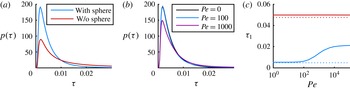
In figure 2(a) we show the probability distribution
 $p(\unicode[STIX]{x1D70F})$
of the residence time at
 $Pe=100$
. In the presence of the sphere the distribution is rather narrow with a sharp peak at
 $\unicode[STIX]{x1D70F}\approx 0.002$
. Comparing with the case when a substance is released at the same position (
 $r=0.9$
) in pure Poiseuille flow the peak height is approximately twice as large. This can be understood by the reflecting boundary conditions on the sphere surface.
The influence of the flow can be seen by varying the Péclet number as in figure 2(b). When removing the flow (
 $Pe=0$
), the distribution remains almost unaltered. Increasing the flow to
 $Pe=1000$
slightly smears out the distribution, but in general the effects of
 $Pe$
on the residence time distribution are not as strong as they are on the reaction position as will be shown below.
This is also seen in figure 2(c) where the mean residence time
 $\unicode[STIX]{x1D70F}_{1}$
is plotted as function of
 $Pe$
for the two situations with and without sphere shown in figure 2(a). In the absence of the sphere
 $\unicode[STIX]{x1D70F}_{1}$
(which is scaled by the radial diffusion time
 $r_{c}^{2}/D$
) is constant and independent of
 $Pe$
since the pure Poiseuille flow has no radial components. In the presence of the sphere, however, this simple scaling breaks down and two plateaus at low and high
 $Pe$
can be discerned. Interestingly, even for very large
 $Pe$
the mean residence time in the presence of the sphere does not reach the one without the sphere. This observation may seem surprising at first since the very fast flow should quickly pull the substance away from the sphere leading to unhindered diffusion. Inspection of figure 1(c) however shows that the effect can be explained by two characteristics of the flow profile in the region behind the sphere into which the substance is dragged: (i) the radial flow is directed outwards and will thus push the substance in direction of the cylinder wall and (ii) if the solute molecule slightly diffuses towards the channel centre, the flow pushes it back onto the reflecting surface of the sphere. We will come back to this point in more detail in § 3.3.
(a) Residence time probability distribution at
 $Pe=100$
for substance released from the equator of a flowing sphere compared to release at
 $r=0.9$
in pure Poiseuille flow. (b) While lowering the flow speed to
 $Pe=0$
has only a slight effect, increasing it to
 $Pe=1000$
leads to a reduction of the peak height. (c) Without the sphere the mean residence time
 $\unicode[STIX]{x1D70F}_{1}$
is independent of
 $Pe$
, while in the presence of the sphere two plateau values at small and high
 $Pe$
can be observed. Dotted lines represent analytical solutions for diffusion between two infinitely long cylinders at
 $Pe=0$
.

We finally give, for
 $Pe=0$
, an estimate of the mean residence time using a theoretical development for diffusion of a substance between two infinitely long concentric cylinders with radii 1 and
 $r_{i}<1$
. As shown by Szabo, Schulten & Schulten (Reference Szabo, Schulten and Schulten1980) and Deutch (Reference Deutch1980) (see also the review by Hänggi et al. (Reference Hänggi, Talkner and Borkovec1990)), the mean residence time when starting at
 $r$
can be obtained from the solution to the one-dimensional differential equation
 $$\begin{eqnarray}\frac{\text{d}^{2}\unicode[STIX]{x1D70F}_{1,cyl}(r)}{\text{d}r^{2}}=-1,\end{eqnarray}$$
with boundary conditions
 $$\begin{eqnarray}\displaystyle \frac{\text{d}\unicode[STIX]{x1D70F}_{1,cyl}}{\text{d}r} & = & \displaystyle 0\quad \text{at}~r=r_{i},\end{eqnarray}$$
 $$\begin{eqnarray}\displaystyle \unicode[STIX]{x1D70F}_{1,cyl} & = & \displaystyle 0\quad \text{at}~r=1.\end{eqnarray}$$
Taking the radius of the inner cylinder the same as the sphere radius,
 $r_{i}=R_{s}=0.9$
, the analytical solution of (3.2) yields
 $\unicode[STIX]{x1D70F}_{1,cyl}=0.0048$
. If the sphere is removed by setting
 $r_{i}=0$
but the substance is still released at
 $r=0.9$
, equation (3.2) can be used to compute the corresponding mean residence time
 $\unicode[STIX]{x1D70F}_{r=0.9}=0.0475$
. Both values are in very good agreement with the numerical solution of the full Fokker–Planck equation at
 $Pe=0$
as can be seen by the dotted lines in figure 2(c) in the presence/absence of the sphere. Even up to fairly large
 $Pe\approx 100$
the solute dispersion in the gap between the sphere and the wall is fairly uninfluenced by the flow.
We finally consider the amount of substance remaining in the cylinder at a given time
 $t$
after release. This quantity can be calculated directly from the residence time distribution as
 $$\begin{eqnarray}C(t)=1-\int _{0}^{t}p(\unicode[STIX]{x1D70F})\,\text{d}\unicode[STIX]{x1D70F}.\end{eqnarray}$$
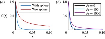
The result in figure 3 shows that (i) the presence of the sphere strongly accelerates the clearance of substance from the channel and (ii) stronger convection slows down, albeit only slightly, the clearance process.
The amount of substance remaining in the channel after a time
 $t$
.

3.2 Reaction position for equatorial release
We now turn to investigate the probability distribution of the reaction position
 $\unicode[STIX]{x1D701}$
on the cylinder wall which is defined as
 $$\begin{eqnarray}p(\unicode[STIX]{x1D701})=2\unicode[STIX]{x03C0}\int _{0}^{\infty }j_{r}(r=1,\unicode[STIX]{x1D701},t)\,\text{d}t\end{eqnarray}$$
which is again a normalized quantity with
 $\int _{-\infty }^{\infty }p(\unicode[STIX]{x1D701})\,\text{d}\unicode[STIX]{x1D701}=1$
. While the mean reaction position is rather irrelevant due to the translational invariance along the
 $z$
-direction, the second central moment (standard deviation)
 $\unicode[STIX]{x1D70E}_{\unicode[STIX]{x1D701}}$
represents an important quantity as it determines how much the biochemically active substance is diluted before it reaches the endothelium. A small
 $\unicode[STIX]{x1D70E}_{\unicode[STIX]{x1D701}}$
implies the existence of a hot spot with a high concentration.
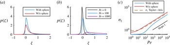
Figure 4(a) shows the distribution
 $p(\unicode[STIX]{x1D701})$
for substance released on the equator of a flowing sphere compared to the case without sphere. The effect of the sphere is to narrow the distribution due to the reflecting boundary condition on the sphere surface which closely mirrors the reduced residence time shown in figure 2(a). As can be seen in figure 4(b) the influence of the flow speed on the reaction position
 $\unicode[STIX]{x1D701}$
is much more pronounced than on the residence time
 $\unicode[STIX]{x1D70F}$
. At
 $Pe=0$
the system possesses a symmetry about the
 $z=0$
plane and accordingly the distribution turns out to be symmetric and rather narrow. At
 $Pe=100$
, the distribution is somewhat smeared out with a strong tendency to higher
 $\unicode[STIX]{x1D701}$
due to advection by the flow. At
 $Pe=1000$
, the peak height lowers quite dramatically and the distribution is much more smeared out.
Indeed, as can be seen by a systematic investigation of the standard deviation
 $\unicode[STIX]{x1D70E}_{\unicode[STIX]{x1D701}}$
as function of
 $Pe$
shown in figure 4(c),
 $\unicode[STIX]{x1D70E}_{\unicode[STIX]{x1D701}}$
is almost uninfluenced by the flow until
 $Pe\approx 100$
, but then rises sharply and finally reaches a regime where it scales linearly with
 $Pe$
. Without the sphere the qualitative picture is the same, yet the transition to the linear regime occurs much earlier and more smoothly.
(a) Probability distribution of the reaction position
 $\unicode[STIX]{x1D701}$
for substance released at
 $Pe=100$
on the equator of a flowing sphere compared to release at
 $r=0.9$
in pure Poiseuille flow. (b) Lowering the flow speed to
 $Pe=0$
sharpens the distribution, while increasing it to
 $Pe=1000$
leads to a significant reduction of the peak height. (c) Width of the reaction position distribution as function of
 $Pe$
. For large
 $Pe$
the width
 $\unicode[STIX]{x1D70E}_{\unicode[STIX]{x1D701}}$
grows linearly with
 $Pe$
in the presence or absence of the sphere. This behaviour is similar to the Taylor–Aris solution. In absolute numbers, the presence of the sphere reduces the width by a factor of approximately 7 compared to the Taylor–Aris solution in the limit of small
 $Pe$
and by a factor of 2.5 in the limit of large
 $Pe$
.

We now draw a connection to the classical Taylor–Aris problem of dispersion in a cylinder with reflecting boundary conditions. The Taylor–Aris solution considers times which are large compared to the diffusive time scale
 $r_{c}^{2}/(4D)$
which in our dimensionless units becomes
 $\unicode[STIX]{x1D70F}_{diff}=0.25$
, and at which therefore all radial concentration differences are negligible. The concentration then becomes a function of
 $z$
only which spreads with a (dimensionless) effective dispersion coefficient
 $$\begin{eqnarray}\displaystyle & \displaystyle D_{TA}=\left(1+\frac{Pe^{2}}{192}\right). & \displaystyle\end{eqnarray}$$
Although not being applicable to perfectly absorbing boundaries, the Taylor–Aris solution nevertheless reproduces one of the characteristic features observed in the present study, namely the linear scaling of
 $\unicode[STIX]{x1D70E}_{\unicode[STIX]{x1D701}}$
with
 $Pe$
in the limit of large
 $Pe$
. To show this, we use
 $D_{TA}$
in a regular diffusion equation and compute the distribution width inside the flow
 $\unicode[STIX]{x1D70E}_{z}$
at
 $\unicode[STIX]{x1D70F}_{diff}$
. The result is shown as the dashed line in figure 4(c) and agrees qualitatively with our numerical data at large
 $Pe$
. Nevertheless, in the large
 $Pe$
regime, the Taylor–Aris solution overestimates the width by a factor of approximately 2.5. At low
 $Pe$
, the deviation is even larger. This demonstrates that the presence of the drug releasing sphere is important over the entire range of Péclet numbers.
(a) Mean residence time as a function of the release position for
 $Pe=0$
,
 $Pe=100$
and
 $Pe=1000$
. While at
 $Pe=0$
the situation is perfectly symmetric, at
 $Pe=1000$
an upstream (
 $\unicode[STIX]{x1D703}_{0}<\unicode[STIX]{x1D703}_{c}\approx 1.1$
) and a downstream region (
 $\unicode[STIX]{x1D703}_{0}>\unicode[STIX]{x1D703}_{c}$
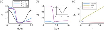
) can be distinguished. Analytical solutions for free diffusion and diffusion between two cylinders are shown as dotted lines and approximate surprisingly well the behaviour in the two regions. (b) The width of the reaction position shows similar behaviour. (c) Mean distance from the moving sphere centre for release on the equator, the front and the tail.

3.3 Influence of release position
We now turn to investigate changes to the above observations when the substance is released at other positions than the equator. For this, we denote the positions by their polar angle starting with
 $\unicode[STIX]{x1D703}_{0}=0$
at the front of the sphere as illustrated in figure 1(b).
In figure 5(a) the mean residence time is shown as function of the release position. At
 $Pe=0$
the system is symmetric around
 $\unicode[STIX]{x1D703}_{0}=\unicode[STIX]{x03C0}/2$
with the smallest
 $\unicode[STIX]{x1D70F}_{1}$
at
 $\unicode[STIX]{x1D703}_{0}=\unicode[STIX]{x03C0}/2$
, i.e., for equatorial release. At higher
 $Pe$
the distribution becomes strongly asymmetric and at
 $Pe=1000$
separates clearly into two regions with almost constant values. In the upstream region for
 $\unicode[STIX]{x1D703}_{0}<\unicode[STIX]{x1D703}_{c}\approx 1.1$
, the mean residence time almost equals that of free diffusion in the absence of the sphere while for
 $\unicode[STIX]{x1D703}_{0}>\unicode[STIX]{x1D703}_{c}$
the mean residence time decreases abruptly to around
 $\unicode[STIX]{x1D70F}_{1}\approx 0.009$
and is thus only slightly larger than the theoretical value for diffusion between two cylinders
 $\unicode[STIX]{x1D70F}_{cyl}=0.0048$
computed from (3.2). A similar behaviour is seen for
 $\unicode[STIX]{x1D70E}_{\unicode[STIX]{x1D701}}$
in figure 5(b). This separation into two regions can be understood from the appearance of the separating streamline in front of the sphere and the flow properties in figure 1(c) as follows. (i) For large
 $z$
the Poiseuille profile needs to be recovered which implies that the velocity on the central axis increases from
 $U_{s}$
to 1 when going away from the front of the sphere. Consequently, a solute molecule close to the front of the sphere will be dragged away from the sphere. (ii) Due to the symmetry of the flow profile, the same increase from
 $U_{s}$
to 1 occurs when going to
 $z=-\infty$
. Thus, a solute molecule released around the tail will, instead of being dragged away, be pushed towards the sphere. This asymmetry in solute behaviour is the cause of the different behaviour in the two regions. (iii) Since the net flow through the gap between sphere and cylinder wall is negative relative to the sphere, a particle released at a position
 $\unicode[STIX]{x1D703}_{0}$
even slightly smaller than
 $\unicode[STIX]{x03C0}/2$
, but still above the separating streamline, will be dragged into the region behind the sphere. This latter property explains why the transition between the two regions is not located strictly at
 $\unicode[STIX]{x03C0}/2$
, but at the smaller value of
 $\unicode[STIX]{x1D703}_{c}\approx 1.1$
.
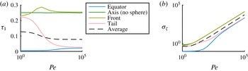
(a) Mean residence time as function of the Péclet number for release on the front and tail of a flowing sphere compared to release on the axis in pure Poiseuille flow and for release on the equator. While substance released at the front behaves very much like substance released in pure Poiseuille flow, a significant influence of the sphere is found for substance released around the tail and the equator. (b) The width of the reaction position shows similar behaviour.

We further illustrate this behaviour by picking the front (
 $\unicode[STIX]{x1D703}_{0}=0$
) and the tail (
 $\unicode[STIX]{x1D703}_{0}=\unicode[STIX]{x03C0}$
) of the sphere as the most obvious prototypes for the upstream and downstream regions. Figure 5(c) shows the mean distance in flow direction from the (moving) sphere centre
 $$\begin{eqnarray}\text{d}_{s}(t)=\int _{V}c(x-U_{s}t,y,z,t)\left(x-U_{s}t\right)\,\text{d}V\end{eqnarray}$$
as a function of time. For front release the substance is advected away from the sphere in positive direction, while for tail release it moves much slower and away from the sphere in the negative direction. Apart from a short initial transient substance released at the equator follows the same behaviour as tail release.
We now turn to investigate the influence of the flow strength on
 $\unicode[STIX]{x1D70F}_{1}$
and
 $\unicode[STIX]{x1D70E}_{\unicode[STIX]{x1D701}}$
for front and tail release. Since both positions are located on the central cylinder axis, we discern the influence of the sphere by comparing to the case where the substance is released on the axis in pure Poiseuille flow. Figure 6(a) shows the mean residence time
 $\unicode[STIX]{x1D70F}_{1}$
for these three situations. In pure Poiseuille flow, the value is simply constant and equal to
 $\unicode[STIX]{x1D70F}_{diff}=0.25$
. As reasoned above, a substance released at the front will quickly be dragged away from the sphere and then experience free diffusion such that
 $\unicode[STIX]{x1D70F}_{1}$
quickly reaches a plateau identical to the one for free diffusion. For tail release, the situation is very different. A rather strong influence of the Péclet number is seen reducing the mean residence time from
 ${\approx}0.25$
at
 $Pe=0$
by almost an order of magnitude at
 $Pe=10^{5}$
. Near the sphere tail the substance is strongly pressed against the sphere by the incoming flow. Furthermore, in the downstream region a small, but non-negligible outward radial flow is present which further accelerates the substance’s motion towards the cylinder wall. These two effects explain the
 $Pe$
-dependence of
 $\unicode[STIX]{x1D70F}_{1}$
in the downstream region.
In an experimental situation it will be difficult to control the precise point of substance release or, equivalently, substance molecules may be released homogeneously over the entire sphere surface. We therefore calculate the mean residence time and the width of the reaction position for a weighted average over release angles
 $0<\unicode[STIX]{x1D703}_{0}<\unicode[STIX]{x03C0}$
covering the entire sphere surface. This is shown by the dashed black lines in figure 6 and demonstrates the non-negligible influence of the sphere in the present problem.
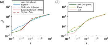
Width of the cross-sectionally averaged distribution inside the flow for a reflecting cylinder wall. The green line in (a) shows axial release in an empty channel and is in perfect agreement with three regimes predicted by Latini & Bernoff (Reference Latini and Bernoff2001) (red lines, see main text). The blue line is for a substance released from the equator of a flowing sphere. (b) Substance released from the front and tail of a flowing sphere.

3.4 Reflecting boundaries
We now investigate the influence of the sphere if the channel walls are reflecting, i.e. we replace the boundary condition (2.3) by
 $$\begin{eqnarray}\displaystyle j_{r} & = & \displaystyle 0\quad \text{at}~r=1.\end{eqnarray}$$
In this situation, the mean residence time
 $\unicode[STIX]{x1D70F}_{1}$
becomes infinite and the reaction position is undefined. We therefore choose the time-dependent width (second central moment)
 $\unicode[STIX]{x1D70E}_{z}(t)$
of the cross-sectionally averaged concentration inside the flow as our quantity of interest. This quantity is similar, but not identical, to
 $\unicode[STIX]{x1D70E}_{\unicode[STIX]{x1D701}}$
for the absorbing channel and allows us to make comparison to a number of earlier works, namely those by Taylor (Reference Taylor1953) and Aris (Reference Aris1956) for long times and by Latini & Bernoff (Reference Latini and Bernoff2001) for short and intermediate times. Figure 7(a) shows
 $\unicode[STIX]{x1D70E}_{z}(t)$
as a function of time for release on the axis in an empty channel. The dotted, dashed and solid red lines denote purely diffusive scaling
 $\unicode[STIX]{x1D70E}_{z}=\sqrt{2t}$
, the anomalous prediction by Latini & Bernoff (Reference Latini and Bernoff2001)
 $\unicode[STIX]{x1D70E}_{z}=\sqrt{8/3}\,Pe\,t^{2}$
and finally the classical Taylor–Aris scaling
 $\unicode[STIX]{x1D70E}_{z}=\sqrt{2D_{eff}t}$
, respectively. We find perfect agreement with those three predictions. Considering next the situation where the substance is released on the equator of the sphere, we find that for large times the Taylor–Aris regime is recovered. However, the dimensionless times required are of the order of 10 which is much higher than the mean residence times
 $\unicode[STIX]{x1D70F}_{1}$
found in the case of absorbing boundaries. This underlines again that the Taylor–Aris scenario is not applicable for strongly absorbing boundaries. At short times, the presence of the sphere is seen to accelerate the deviation from the purely molecular diffusive regime which can be attributed to the rather large shear rates in the vicinity of the equator (cf. figure 1
c).
In figure 7(b) we show release from the front and tail positions of the sphere. Similarly as before with absorbing walls, we find that substance released from the front is quickly dragged away from the sphere and therefore the situation without sphere is recovered even before the Taylor–Aris regime is reached. For tail release, the sphere influence is much more pronounced. At short times, there exists a regime during which the dispersion is almost zero illustrating the pushing of the substance towards the sphere by the flow. Afterwards, a sharp increase in the width is seen when the substance starts to diffuse radially away from the sphere surface. Finally, the Taylor–Aris regime is recovered, albeit more slowly than for release from the front.
3.5 Continuous release
In this final part, we consider a sphere continuously releasing substance at a rate
 $w$
. As the substance molecules are non-interacting, the residence time distribution for a single molecule is identical to the instantaneous release studied above and given by
 $p(\unicode[STIX]{x1D70F})$
. As a novel observable in the continuous release scenario, we investigate the time-dependent absorption rate observed at a fixed position as the sphere passes by. Without restriction of generality we choose the observation position at
 $z=0$
and consider a sphere having started its trajectory at
 $t\rightarrow -\infty$
, passing the observation point at
 $t=0$
and continuing its trajectory until
 $t\rightarrow \infty$
. Due to the linearity of the underlying (2.1), the continuous release scenario can be studied in a Green’s function like approach by superposing data obtained for the instantaneous release. For this, we introduce the flux
 $j^{\ast }$
through the entire cylinder circumference (per unit length in
 $z$
and per unit time) which is observed at
 $z$
,
 $t$
if the sphere has released a unit amount of substance at
 $z_{0}$
,
 $t_{0}$
. This can be related to our previous notation by integrating the flux over the azimuthal angle which (for a normalized cylinder radius of 1) yields
 $$\begin{eqnarray}j^{\ast }(z_{0},z,t_{0},t)=2\unicode[STIX]{x03C0}j_{r}(z-z_{0},t-t_{0}).\end{eqnarray}$$
The total flux per unit length and time at
 $z=0$
is then given by superposing the contributions from all releases that have taken place since
 $t\rightarrow -\infty$
:
 $$\begin{eqnarray}\displaystyle a(t) & = & \displaystyle w\int _{-\infty }^{t}j^{\ast }(U_{s}t^{\prime },0,t^{\prime },t)\,\text{d}t^{\prime }\end{eqnarray}$$
 $$\begin{eqnarray}\displaystyle & = & \displaystyle 2\unicode[STIX]{x03C0}w\int _{-\infty }^{t}j_{r}(-U_{s}t^{\prime },t-t^{\prime })\,\text{d}t^{\prime }.\end{eqnarray}$$
Substituting
 $\hat{t}=t-t^{\prime }$
yields finally
 $$\begin{eqnarray}\displaystyle & \displaystyle a(t)=2\unicode[STIX]{x03C0}w\int _{0}^{\infty }j_{r}(-U_{s}(t-\hat{t}),\hat{t})\,\text{d}\hat{t} & \displaystyle\end{eqnarray}$$
which can conveniently be computed using the instantaneous release condition on a ring studied in the previous sections. Due to mass conservation in a very long cylinder at steady state the total amount of substance absorbed by per unit length of channel wall must equal the amount of substance released per unit length by the sphere, i.e.
 $$\begin{eqnarray}\int _{-\infty }^{\infty }a(t)\,\text{d}t=\frac{w}{U_{s}}.\end{eqnarray}$$
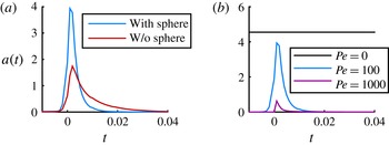
In figure 8(a) we show
 $a(t)$
for the same parameters as in the instantaneous release scenario (
 $R_{s}=0.9$
). We first note that there is a strong asymmetry around the passing moment
 $t=0$
. Just before
 $t=0$
the signal rises sharply due to substance diffusing up front relative to the approaching sphere. The maximum signal is reached for
 $t$
slightly larger than 0 and then decays slowly which is due to convection of the substance into the region behind the sphere as described in detail above. Comparing to a hypothetical continuous release from a moving ring source (without sphere), we observe that the signal picked up at
 $z=0$
becomes narrower due to the presence of the sphere. This is fully in line with the results derived above for the instantaneous injection.
Finally, in figure 8(b) we show a comparison for three different Péclet numbers. For
 $Pe=0$
the sphere does not move and therefore the signal has no time dependence. Increasing
 $Pe$
from 100 to 1000 leads to a smaller and sharper peak.
The absorption rate per unit length and time observed at
 $z=0$
for a sphere passing at
 $t=0$
. In this scenario, the sphere continuously releases substance. (a) The presence of the sphere sharpens the signal. (b) Increasing
 $Pe$
leads to a smaller peak height in line with (3.14).

4 Conclusion
We studied the dispersion of a solute released from the surface of a sphere flowing freely through a cylindrical channel with absorbing boundary conditions on the channel wall. Since the sphere velocity is slower than the centre velocity of the undisturbed Poiseuille flow at
 $z\rightarrow \pm \infty$
two regimes can be distinguished. In the upstream regime the solute is released around the front of the sphere and then quickly washed away from the sphere by the flow and free diffusion is recovered at large Péclet numbers. In the downstream regime the solute is pushed towards the sphere leading to a strong reduction in residence time and a peaked reaction position distribution. These effects can be attributed to the reflecting boundary on the sphere surface but also to the radially outward component of the flow field behind the sphere which acts to push the solute towards the channel wall. Even at very large
 $Pe$
, free diffusion is not recovered in the downstream regime. The transition between both regimes is smooth at low
 $Pe$
and becomes increasingly sharper at higher
 $Pe$
. The important case of equatorial release which incorporates the largest surface area always belongs to the downstream regime.
Acknowledgements
I thank the Volkswagen Foundation for financial support in the framework of the Lichtenberg programme. I acknowledge the Gauss Center for Supercomputing e.V. for providing computing time on the GCS Supercomputer SuperMUC at Leibniz Supercomputing Center.
Supplementary materials
Supplementary materials are available at https://doi.org/10.1017/jfm.2017.177.
Appendix A. Analytical computation of the flow field around a sphere travelling through a channel
Here we briefly recall the calculation of the axisymmetric flow field when a sphere travels force free along the centre of a cylindrical channel. The details are given by Leichtberg et al. (Reference Leichtberg, Pfeffer and Weinbaum1976) and Yeh & Keh (Reference Yeh and Keh2013). The key idea is to find a general solution to the Stokes equation satisfying exactly the boundary conditions at infinity and on the cylinder surface, but not necessarily on the sphere surface. The free constants in this solution as well as the sphere velocity are then determined by enforcing the no-slip condition on a set of points on the sphere surface. The number of such collocation points determines the accuracy of the result. We note here that the second occurrence of
 $G_{n+1}^{-1/2}(\unicode[STIX]{x1D705})$
in equation (A 1) of Yeh & Keh (Reference Yeh and Keh2013) should actually read
 $G_{n}^{-1/2}(\unicode[STIX]{x1D705})$
Appendix B. Separating streamline
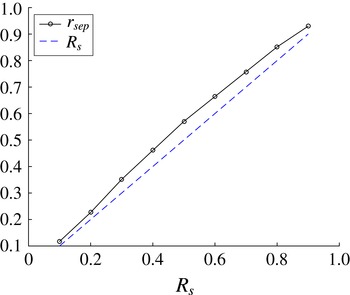
In figure 9 we show the radial starting position of the separating streamline
 $r_{sep}$
at
 $z\rightarrow \infty$
as a function of the sphere radius
 $R_{s}$
. Both quantities are very similar over the whole range of sphere radii.
Radial position of the separating streamline as a function of sphere radius.