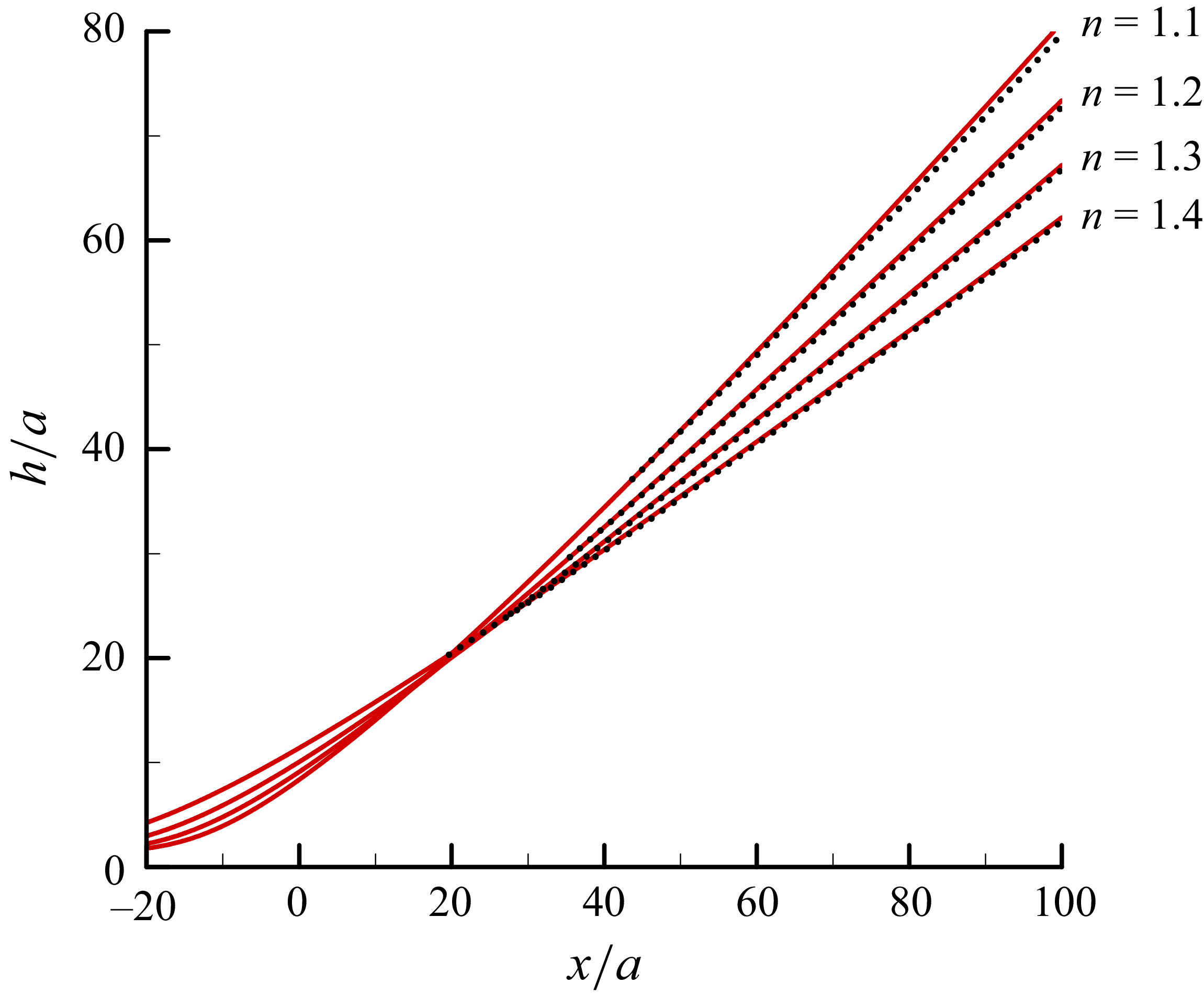
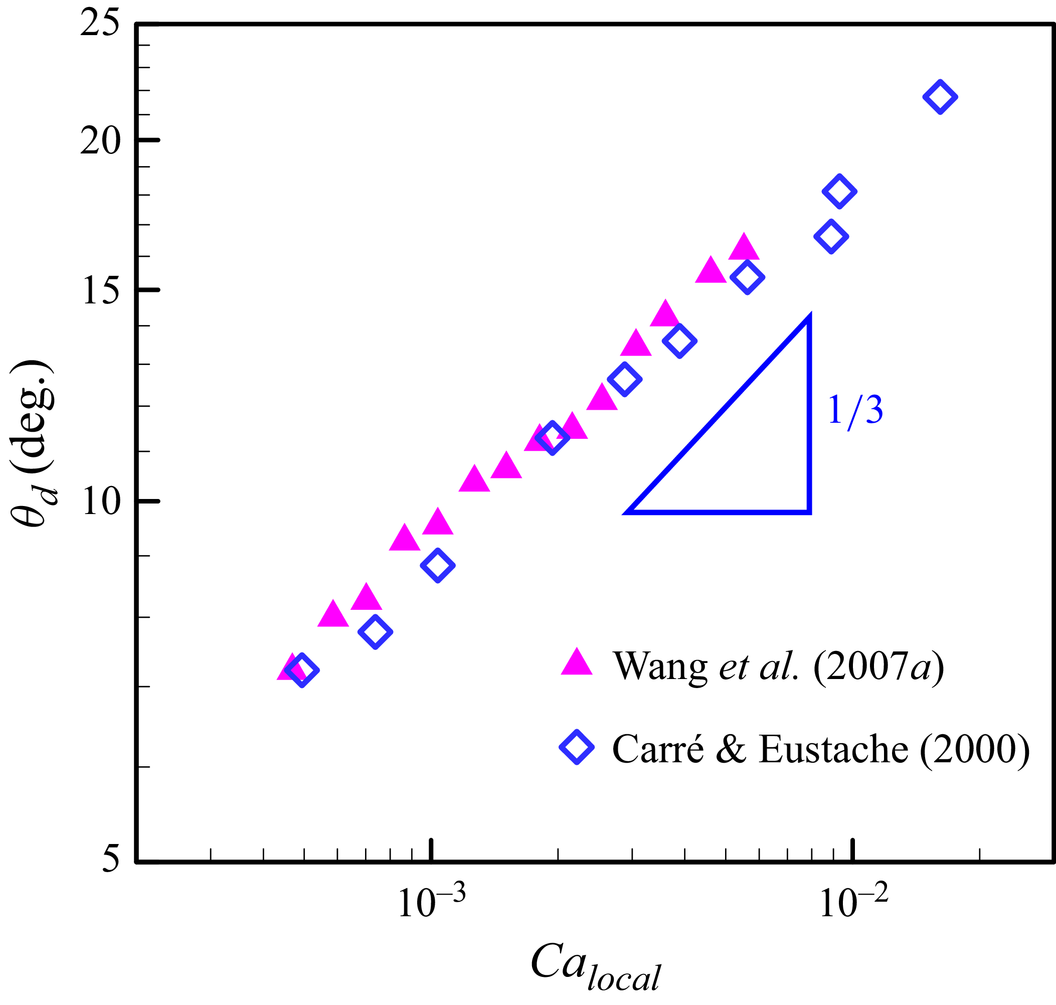
1. Introduction
When a liquid droplet is placed on a substrate, it spreads due to surface tension effects, driven by the three-phase moving contact line at its expanding periphery. In various applications such as coating, painting, printing and spraying, this local contact line motion plays a crucial role in dynamic wetting, as it directly influences the overall spreading behaviour. The motion of a contact line is often characterised by the relationship of the apparent dynamic contact angle
 $\theta _{d}$
to the contact line speed
 $U$
. A well-known example is the Cox-Voinov law for complete wetting Newtonian fluids, which states that
 $\theta _{d}\propto U^{1/3}$
(Voinov Reference Voinov1976; Cox Reference Cox1986). This, in turn, leads to the spreading radius
 $R$
evolving over time
 $t$
according to Tanner’s law
 $R\propto t^{1/10}$
(Tanner Reference Tanner1979). A broader discussion on dynamic wetting and spreading, including further developments, can be found in review articles (De Gennes Reference de Gennes1985; Bonn et al. Reference Bonn, Eggers, Indekeu, Meunier and Rolley2009; Snoeijer & Andreotti Reference Snoeijer and Andreotti2013).
In practice, however, many liquids such as polymer solutions are not Newtonian. The simplest type of such liquids is a power-law fluid, whose viscosity η varies with shear rate
 $\dot{\gamma }$
as η = k
 $\dot{\gamma }$
n−1, where n is the rheological exponent with n < 1 for shear-thinning fluids and n > 1 for shear-thickening fluids, and k is the consistency constant. In this paper we focus on how this power-law rheology influences the behaviour of the dynamic contact angle
 $ \theta_{d}$
under the complete wetting condition where
 $ \theta_{d}$
is governed solely by hydrodynamic mechanisms and remains independent of the substrate’s wettability or the spreading coefficient (Bonn et al. Reference Bonn, Eggers, Indekeu, Meunier and Rolley2009). We pay particular attention to this topic not only because the explicit relationship between dynamic contact angle
 $\theta _{d}$
and contact line speed U – analogous to the De Gennes–Tanner–Cox–Voinov framework for Newtonian fluids has not yet been rigorously derived for power-law fluids, but also because this relationship is more fundamental than the spreading law, as knowing the former can determine the latter, but not vice versa. More importantly, deriving the dynamic contact relationship requires directly addressing the stress singularity at the contact line. This poses significant theoretical challenges and raises the following key questions.
-
(i) How does the nature of the contact stress singularity change due to power-law rheology? Does the singularity become milder or more severe, and does the resulting contact force remain finite or continue to diverge, in contrast to the classical Huh–Scriven paradox for Newtonian fluids (Huh & Scriven Reference Huh and Scriven1971)?
-
(ii) How does the contact line structure respond to the change of the singularity?
-
(iii) How is the precursor film contact line microstructure – arising from molecular disjoining pressure, a microscopic mechanism that alleviates the contact line singularity when necessary – modified by the power-law rheology?
Answering these questions is not only of fundamental importance for understanding non-Newtonian wetting dynamics, but also has broader implications, extending beyond droplet spreading and capillary wetting to other interfacial processes involving contact lines (Charitatos et al. Reference Charitatos, Suszynski, Carvalho and Kumar2020). We aim to extend and refine previous efforts by filling these gaps and providing a clearer, more general framework for describing contact line dynamics in power-law fluids.
Rigorous theoretical analysis based on the fundamental lubrication equations to elucidate the differences between power-law fluids and Newtonian fluids was first carried out by King (Reference King2001). Betelu & Fontelos (Reference Betelu and Fontelos2003) derived the evolution equation for spreading power-law fluids in planar geometry and demonstrated that solutions have bounded dissipation rates. For spreading shear-thinning drops, in particular, the spreading law
 $R\propto t^{n/(3n+7)}$
was subsequently obtained with complete prefactors using self-similar analysis under the constraint of constant drop volume (Starov et al. Reference Starov, Tyatyushkin, Velarde and Zhdanov2003; Betelu & Fontelos Reference Betelu and Fontelos2004; Rafaï et al. Reference RafaÏ, Bonn and Boudaoud2004). The corresponding evolution of the dynamic contact angle
 $ \theta_{d}(t)$
can also be obtained. Both the spreading law and the contact angle evolution are found to differ markedly from those of Newtonian fluids. What is more important is that there is no divergence issue in the contact line force (King Reference King2001; Betelu & Fontelos Reference Betelu and Fontelos2004; Rafaï et al. Reference RafaÏ, Bonn and Boudaoud2004). In fact, this feature was first identified by Weidner & Schwartz (Reference Weidner and Schwartz1994) in their analysis of the contact line motion of a vertically draining film and was later confirmed by Carré & Woehl (Reference Carré and Woehl2002). Rafaï et al. (Reference RafaÏ, Bonn and Boudaoud2004) further conducted drop experiments with shear-thinning fluids, showing that the measured spreading exponents are in reasonable agreement with the values predicted by such self-similar analysis. Similar experimental trends were subsequently reported by Wang et al. (Reference Wang, Zhang, Lee and Peng2007b
) and Min et al. (Reference Min, Duan, Wang, Liang, Lee and Su2010).
Despite these previous efforts, several important aspects remain to be further developed. First, while the spreading law itself has been established, the physical mechanism connecting the microscopic contact line behaviour to macroscopic spreading via an explicit characteristic length scale has not been fully quantified. Second, for shear-thickening fluids – where regularisation at the contact line is required (King Reference King2001) – the detailed contact line microstructure and how it matches to the macroscopic wedge remains unresolved. Third, the relationship between the dynamic contact angle and contact line speed – which is more fundamental than the spreading law – has yet to be rigorously derived from the hydrodynamic equations in a manner analogous to the De Gennes–Tanner–Cox–Voinov framework for Newtonian fluids. The difficulty likely stems from the highly nonlinear structure of the lubrication equations governing the contact line, which involve fractional powers of the film thickness. This nonlinearity may preclude analytically tractable treatments capable of revealing the detailed contact line structure needed to formulate a physically consistent description of the dynamic contact angle.
Various attempts to address the last issue have been made. Several dynamic contact angle models for power-law fluids have been proposed (Carré & Eustache Reference Carré and Eustache2000; Wang et al. Reference Wang, Lee, Peng and Lai2007a ; Dandapat & Singh Reference Dandapat and Singh2010; Liang et al. Reference Liang, Wang, Duan and Min2012; Wang et al. Reference Wang, Min, Zhang and Duan2018), but they are either somewhat incomplete or lack consistency. For instance, some models suggest that the dynamic contact angles of both shear-thinning and shear-thickening fluids follow the same power-law form with respect to contact line speed, differing only in their coefficients (Wang et al. Reference Wang, Lee, Peng and Lai2007a ; Liang et al. Reference Liang, Wang, Duan and Min2012; Wang et al. Reference Wang, Min, Zhang and Duan2018). However, this is unlikely, as the dissipation mechanisms differ between the two cases. In shear-thinning fluids, dissipation primarily occurs in the bulk (King Reference King2001; Carré & Woehl Reference Carré and Woehl2002; Rafaï et al. Reference RafaÏ, Bonn and Boudaoud2004), whereas in shear-thickening fluids, dissipation is concentrated at the contact line (King Reference King2001; Wang & Zhu Reference Wang and Zhu2014). Another unsettled issue is that most of these models fail to explain the spreading kinetics found in rigorous theoretical analyses (Starov et al. Reference Starov, Tyatyushkin, Velarde and Zhdanov2003; Betelu & Fontelos Reference Betelu and Fontelos2004). Perhaps the most problematic inconsistency is that, even for the same power-law fluid type, different models predict conflicting dependences on the contact line speed (Min et al. Reference Min, Duan, Wang, Liang, Lee and Su2010).
It is worth noting that Wang et al. (Reference Wang, Lee, Peng and Lai2007a
) solved the lubrication equation and obtained the dynamic contact angle relationships for both shear-thinning and shear-thickening fluids. In their expressions, a microscopic cutoff was introduced to remove the contact line singularity. However, such a microscopic cutoff is unnecessary for shear-thinning fluids, as there is no divergence in viscous dissipation that mainly occurs in the bulk (King Reference King2001; Carré & Eustache Reference Carré and Eustache2000; Rafaï et al. Reference RafaÏ, Bonn and Boudaoud2004; Wang & Zhu Reference Wang and Zhu2014). For shear-thickening fluids, on the other hand, Wang et al. (Reference Wang, Lee, Peng and Lai2007a
) introduced a microscopic cutoff length
 $x_{m}$
to mitigate the much more severe contact line singularity, evaluating the dynamic contact angle at a fixed
 $x_{m}$
. However, keeping
 $x_{m}$
fixed implies that the corresponding contact line microstructure is rate independent, which is generally not the case. Wang & Zhu (Reference Wang and Zhu2014) developed a scaling theory to address this issue. But a detailed description for the contact line microstructure and how it matches to the macroscopic wedge are still lacking.
Considering the above, developing a rigorous hydrodynamic theory is essential for a consistent explanation for the contact line motion of both shear-thinning and shear-thickening fluids. Specifically, we aim to extend the classical De Gennes–Tanner–Cox–Voinov framework to power-law fluids, thereby providing a comprehensive description of their wetting dynamics. Such a framework will not only reveal how
 $\theta _{d}$
varies quantitatively with
 $U$
and account for the spreading laws reported in previous studies but also clarify how relevant length scales influence the interface behaviour near and away from the contact line. This understanding crucially depends on how the nature of the contact line stress singularity is affected by fluid rheology, and highlights its plausible microscopic mechanisms, if necessary, to alleviate the singularity (De Gennes Reference de Gennes1985; Eggers & Stone Reference Eggers and Stone2004; Wei, Tsao & Chu Reference Wei, Tsao and Chu2019).
In this work we aim to establish a unified theoretical framework to account for distinct contact line characteristics of shear-thinning and shear-thickening fluids, arising from their fundamentally different stress singularity behaviours. To achieve this, this paper is structured to develop the ideas progressively and transparently. We begin with the basic physical picture and a scaling analysis to identify the key features at a qualitative level. Building on this foundation, we then construct a rigorous formulation for a quantitative description and proceed to a deeper exploration as our level of understanding advances.
Specifically, § 2 first reviews the classical De Gennes–Tanner–Cox–Voinov theory for Newtonian fluids, which serves as a baseline for comparison and later generalisation for power-law fluids. Section 3 provides an overview and conceptual sketch elucidating how and why the nature of a stress singularity – through the rheological exponent n – governs the extent of viscous dissipation and, consequently, the characteristics of moving contact lines. Building on this understanding, we derive the apparent dynamic contact angle relationships in simple scaling forms without directly solving the governing equations. This offers physical insights into how the apparent dynamic contact angle depends on the contact line speed and the fluid rheology, thereby laying the groundwork for the rigorous theoretical derivations presented in §§ 4 and 5. In § 4 we derive the equations governing the contact line motion and identify the emergence of a characteristic dissipation length that controls the extent of viscous dissipation. The corresponding apparent dynamic contact angle relationships are also obtained, showing that this length plays a central role in determining the dynamic contact angle behaviour. This further highlights that the Newtonian fluid represents a special case, as it lacks such a characteristic dissipation length. In § 5 we develop a complete precursor film theory to provide the necessary microscopic cutoff for shear-thickening fluids, which exhibit more strongly diverging contact line forces, and demonstrate how the resulting microscopic structure connects to the macroscopic wetting behaviour. Section 6 compares our theoretical predictions with experiments. Section 7 summarises the key findings and presents concluding remarks.
2. Review of the classical De Gennes–Tanner–Cox–Voinov theory for Newtonian fluids
Before investigating the effects of power-law rheology on dynamic wetting, it is useful first to revisit the classical Newtonian framework and outline its fundamental characteristics.
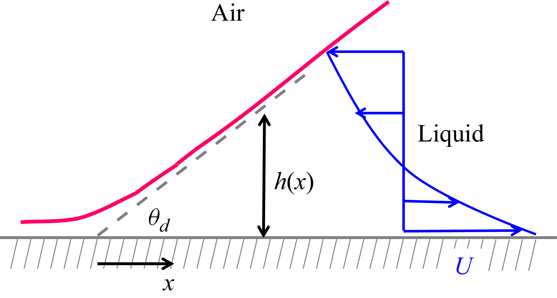
Schematic picture of an advanced contact line motion in the comoving frame.

Consider the advancing motion of a contact line having a small contact angle
 $\theta _{d}$
in a wedge geometry (see figure 1) and start by reviewing some fundamental aspects for the Newtonian case. How the local liquid profile
 $h(x)$
varies with distance
 $x$
to the contact line can be described by the well-known Tanner equation, derived using lubrication theory (Tanner Reference Tanner1979):
 \begin{align} h^{\prime \prime \prime}=-\frac{3\textit{Ca}}{h^{2}} .\end{align}
Here
 $ \textit{Ca}=\eta U/\gamma$
is the capillary number with
 $\gamma$
being the surface tension. The primes denote derivatives with respect to
 $x$
. Compared with the more generalised equation for power-law fluids (see (4.1) and its derivation in Appendix A), the form of (2.1) is somewhat special, as its solution takes the form (Bonn et al. Reference Bonn, Eggers, Indekeu, Meunier and Rolley2009):
 \begin{align} h=\ell H\left(x/\ell\right) . \end{align}
Equation (2.2) indicates that the slope
 $h^{\prime}$
remains invariant regardless of the characteristic length
 $\ell$
chosen to scale both
 $h$
and
 $x$
. This means that if it is taken as a microscopic length, the local contact line dynamics becomes decoupled from the macroscopic droplet motion. Consequently, the apparent dynamic contact angle
 $\theta _{d}(x)\equiv h^{\prime}$
can be determined at
 $x\gg \ell$
. This separation of length scales ensures that the expression for
 $\theta _{d}$
becomes universal, taking the following asymptotic form with vanishing curvature at infinity,
 \begin{align}h^{\prime 3}\left(x\right)=h^{\prime 3}\left(\ell\right)+9Ca \ln \left(\frac{x}{\ell}\right)\!,\end{align}
which is the well-known Cox-Voinov law (Voinov Reference Voinov1976; Cox Reference Cox1986). As indicated by (2.3),
 $\theta _{d}$
exhibits only a weak dependence on
 $x$
due to the presence of the logarithmic term. This implies that
 $\theta _{d}$
is largely insensitive to macroscopic length scales, aligning with the concept of length scale separation. Similarly, the dependence of
 $\theta _{d}$
on the microscopic length
 $\ell$
is also weak in a logarithmic manner, reflecting scale invariance from (2.2). This logarithmic dependence arises from the integration of the diverging viscous stress
 $\sim \eta U/\theta _{d}x$
at the contact line within the macroscopic wedge (Huh & Scriven Reference Huh and Scriven1971).
Since
 $\theta _{d}$
given by (2.3) approximately follows
 $\theta _{d}\propto U^{1/3}$
(neglecting the microscopic contact angle
 $\theta _{m}\equiv h^{\prime}(\ell)$
), this together with
 $U=\textrm{d}R/\textrm{d}t$
under the constant volume constraint
 $R^{3}\theta _{d}={\Omega}$
renders the spreading radius
 $R$
to evolve as
 $R\propto t^{1/10}$
, which is the well-known Tanner law (Tanner Reference Tanner1979). Thus, as a direct consequence of the local dynamic contact angle relationship, the global spreading law also inherently reflects the fundamental nature of a moving contact line.
When the spreading liquid becomes a power-law type, the viscosity
 $\eta$
is no longer constant but depends on the shear rate, leading to a series of changes in the contact line dynamics. Most notably, the viscous term in (2.1) scales as
 $1/h^{\nu }$
with
 $\nu \neq 2$
. To preserve scale invariance in the solution,
 $x$
must be scaled with a different power of
 $\ell$
than
 $h$
(Boatto, Kadanoff & Olla Reference Boatto, Kadanoff and Olla1993). However, this inevitably causes the slope
 $h^{\prime}$
to strongly depend on
 $\ell$
, meaning that the local contact line dynamics may no longer decouple from the global drop spreading motion. Therefore,
 $\theta _{d}$
and
 $R$
will no longer obey the Cox–Voinov law (2.3) and Tanner’s law. As a result, macroscopic lengths such as drop size or substrate’s curvature may explicitly influence
 $\theta _{d}$
, which has indeed been observed experimentally (Wang et al. Reference Wang, Min, Zhang and Duan2018).
We emphasise that such lack of separation between local wetting and global spreading is not exclusive to power-law fluids. Rather, it is a direct consequence of the absence of scale invariance or separation, which can result from any mechanism that modifies the viscous term in (2.1). Another example of this phenomenon can be seen in the spreading of a slipping drop, especially when the slip length is much larger than the drop height (Wei et al. Reference Wei, Tsao and Chu2019).
3. Conceptual sketch about features of moving contact lines in power-law fluids
Before presenting the rigorous formulation for the dynamic contact angle in § 4, it is useful to examine how the contact line characteristics in power-law fluids are modified and how they differ from those in Newtonian fluids. To this end, we perform a scaling analysis – without directly solving the governing equations – to provide a simple sketch of how the nature of contact line stress singularity influences the force on the contact line and consequently on the dynamic contact angle.
The fluid viscosity is assumed to take the simple power-law form described by the Ostwald–de Waele relationship:
 \begin{align}\eta =k\dot{s}^{n-1}.\end{align}
Here the shear rate
 $\dot{s}=|\partial u/\partial y|$
measures the strength of the velocity gradient in the transverse direction,
 $\partial u/\partial y$
(
 $\lt 0$
in the frame moving with the contact line; see figure 1). As will be shown below, although the viscous stress always diverges at the contact line, the contact line force may remain finite or diverge even more strongly. This, in turn, alters the contact line structure and, consequently, the dynamic contact angle relationship. It should be noted that some of these analyses have been performed previously (Carré & Eustache Reference Carré and Eustache2000; Carré & Woehl Reference Carré and Woehl2002; Liang et al. Reference Liang, Wang, Duan and Min2012); however, they either focus exclusively on shear-thinning fluids (Carré & Eustache Reference Carré and Eustache2000; Carré & Woehl Reference Carré and Woehl2002) or, in the case of shear-thickening fluids, employ formulations that are not entirely accurate (Liang et al. Reference Liang, Wang, Duan and Min2012). In this section we will not only fill these gaps using a scaling analysis without explicitly solving the hydrodynamic equations but also provide a clear and unified physical picture of the mechanisms behind how the contact line stress and force govern the local structure and the resulting dynamic contact angle.
3.1. Stress singularity versus force singularity: distinct dissipation length scales
To begin, we recognise that even in a power-law fluid, a stress singularity persists at a moving contact line due to a velocity jump between the moving air–liquid interface and the no-slip substrate. This can be seen from the fact that the viscous stress
 $\tau$
with the power index
 $n\gt 0$
diverges as the contact line is approached:
 \begin{align}\tau =\eta \frac{\partial u}{\partial y}=k\left(-\frac{\partial u}{\partial y}\right)^{n}\sim k\left(\frac{U}{h}\right)^{n}\rightarrow \infty\quad\text{as }h\rightarrow 0.\end{align}
However, the viscous braking force F
brake
on the contact line does not necessarily diverge at the contact line as can be seen by integrating (3.2) with respect to
 $x$
. Specifically, with
 $h\approx \theta _{d}x$
, this force (per unit length) for
 $n\neq 1$
, F
brake
behaves as
 \begin{align}F_{\textit{brake}}=k\int _{x_{m}}^{L}\left(-\frac{\partial u}{\partial y}\right)^{n}\,\textrm{d}x\sim k\int _{x_{m}}^{L}\left(\frac{U}{\theta _{d}x}\right)^{n}\,\textrm{d}x=\frac{k}{1-n}\left(\frac{U}{\theta _{d}}\right)^{n}\left[L^{1-n}-x_{m}^{1-n}\right]\!,\end{align}
where
 $L$
is the length of the macroscopic wedge and
 $x_{m}$
(
 $\ll L$
) is a mesoscopic length bridging the macroscopic and microscopic regions. As evident from (3.3), whether
 $F_{\textit{brake}}$
is dominated by
 $L$
or
 $x_{m}$
critically depends on whether
 $n\lt 1$
or
 $n\gt 1$
. The force described by (3.3) is very different than the Newtonian fluid case where the contact line force diverges logarithmically as
 $x_{m}$
→ 0 (De Gennes Reference de Gennes1985):
 \begin{align} F_{\textit{brake}}\left(n=1\right)\sim \frac{\eta U}{\theta _{d}}\ln \left(\frac{L}{x_{m}}\right) \! . \end{align}
As evident from (3.3), F
brake
can still diverge for n > 1 or remain finite for n < 1 as xm
→ 0. When n > 1, the viscosity
 $\eta \sim k (U/h)^{n-1}$
becomes increasingly pronounced as h approaches the contact line, thereby producing a much stronger divergence force of the contact line than that given by (3.4) for the Newtonian case. This causes viscous dissipation to be even more strongly concentrated in the immediate vicinity of the contact line.
In contrast, for n < 1, since the viscosity
 $\eta \propto h^{1-n}$
vanishes at the contact line (h = 0) and increases toward the bulk, the dissipation must extend beyond the contact line region. Consequently, the force is redistributed over a larger portion of the wedge, leading to a finite contact line force that reflects the integrated dissipation throughout the wedge. Similar conclusions can also be drawn from the viscous energy dissipation rate over the wedge (Carré & Woehl Reference Carré and Woehl2002; Liang et al. Reference Liang, Wang, Duan and Min2012), i.e.
 \begin{align}T\dot{\Sigma }_{w}\equiv \int _{x_{m}}^{L}\int _{0}^{h}\eta \left(\frac{\partial u}{\partial y}\right)^{2}\,\textrm{d}y\,\textrm{d}x\sim \frac{k}{1-n}\left(\frac{U}{\theta _{d}}\right)^{n+1}\theta_d\left[L^{1-n}-x_{m}^{1-n}\right]\!,\end{align}
from which (3.3) can be readily recovered using
 $F_{\textit{brake}}\sim T\dot{\Sigma }_{w}/U$
. Both the force and the energy dissipation rate are proportional to the same factor (
 $L^{1-n}-x_m^{1-n}$
), which determines whether viscous effects are localised near the contact line or extend across the wedge. This viscous energy dissipation approach not only reveals that the dominant region of viscous dissipation coincides with that of the contact line force but also provides a picture of how the local stress distribution governs the overall contact line dynamics. In what follows, we discuss the different contact line force characteristics for n < 1 and n > 1.
For shear-thinning fluids (
 $n\lt 1$
), F
brake
described by (3.3) is dominated by the macroscopic
 $L$
term (Carré & Eustache Reference Carré and Eustache2000):
 \begin{align}F_{\textit{brak}\mathrm{e}}(n\lt 1)\sim \frac{k}{1-n}\left(\frac{U}{\theta _{d}}\right)^{n}L^{1-n}.\end{align}
Thus, although the stress exhibits a singularity at the contact line, it is in fact integrable, causing F
brake
to remain finite at the contact line regardless of
 $x_{m}$
. This integrable singularity feature could be easily overlooked, as illustrated, for instance, by Wang et al. (Reference Wang, Lee, Peng and Lai2007a
) who introduced a microscopic cutoff xm
in their derivation of the dynamic contact angle relationship, in a manner analogous to the Newtonian fluid case. It follows, therefore, that since the viscous dissipation is no longer concentrated at the contact line but grows with L, the local contact line motion can be dissipated through the bulk without needing any microscopic cutoff. This feature is consistent with the key characteristics of shear-thinning fluids identified by King (Reference King2001) and Betelu & Fontelos (Reference Betelu and Fontelos2004), who rigorously solved the governing equations. Here we provide a much simpler reasoning and physical argument to re-establish this feature. As will be seen in § 3.2, this will lead to
 $ \theta_{d}$
depending on the extent of spreading.
For shear-thickening fluids (
 $n\gt 1$
), on the contrary, the force (3.3) is mainly controlled by the mesoscopic
 $x_{m}$
term,
 \begin{align}F_{\textit{brake}}\left(n\gt 1\right)\sim \frac{k}{1-n}\left(\frac{U}{\theta _{d}}\right)^{n}x_{m}^{1-n},\end{align}
indicating that F
brake
still diverges as
 $x_{m}$
→ 0. This divergence is of a power-law type and, thus, more severe than the logarithmic divergence (3.4) seen in the Newtonian case. Consequently, a microscopic cutoff is required to alleviate the force singularity at the contact line. The need for such a regularisation at the contact line has also been noted by King (Reference King2001) for the same reason. This necessity also makes the analysis of shear-thickening fluids more challenging and, as a result, less studied.
Characteristic differences between the
 $n\lt 1$
and
 $n\gt 1$
cases have been noticed by Liang et al. (Reference Liang, Wang, Duan and Min2012) from an energy dissipation perspective. However, their expression for viscous dissipation energy followed the bulk dissipation mode (3.6) derived by Carré & Eustache (Reference Carré and Eustache2000) for shear-thinning fluids (
 $n\lt 1$
) and was extended to the shear-thickening case (
 $n\gt 1$
) by introducing an additional dissipation factor to account for the effects of the stress singularity. As a result, their formulas for
 $\theta _{d}$
showed little qualitative difference between these two cases, apart from the dissipation factor. This challenges the notion that their contact line motions are dissipated within different dissipation length scales, as indicated by (3.6) and (3.7). Therefore, their dynamic contact angles must exhibit distinct behaviours, which we demonstrate next.
3.2. Energy dissipation and scaling relationships for
 ${\theta }_{{d}}$

Having obtained the distinct viscous force characteristics (3.6) and (3.7), we now balance each with the surface tension force to derive the corresponding scaling relationships for
 $\theta _{d}$
. This will enable us to reveal essential features of how
 $\theta _{d}$
varies with
 $U$
and the relevant length scales.
The surface tension force that drives the contact line is often expressed as a pulling tension force at the dynamic state relative to the static state with the equilibrium contact angle
 $\theta _{e}(\lt \theta _{d})$
(Carré & Eustache Reference Carré and Eustache2000):
 \begin{align}F_{s}=\gamma (\cos \theta _{e}-\cos \theta _{d}).\end{align}
For small
 $\theta _{d}$
, as in the case of complete wetting, (3.8) simplifies to (De Gennes Reference de Gennes1985)
 \begin{align}F_{s}\approx (\gamma /2)\theta _{d}^{2}+S.\end{align}
Here
 $S=\gamma _{SV}-\gamma _{LS}=\gamma (\cos \theta _{e}-1)\approx -(\gamma /2)\theta _{e}^{2}$
is the spreading coefficient, which measures the excess interfacial free energy per unit area. The terms
 $\gamma _{SV}$
and
 $\gamma _{LS}$
represent the solid–vapour and the liquid–solid interfacial tensions, respectively.
As indicated by (3.9), this surface tension force includes an additional contribution from
 $S$
to account for the wettability of a substrate. In the case of complete wetting, it is well established that for Newtonian fluids, the spreading kinetics described by Tanner’s law remains universal, independent of the value of
 $S$
(Bonn et al. Reference Bonn, Eggers, Indekeu, Meunier and Rolley2009). This implies that
 $S$
does not enter the dynamic contact angle relationship
 $\theta _{d}(U)$
, which also explains the universality of the Cox–Voinov law (2.3).
De Gennes (Reference de Gennes1985) has shown for the Newtonian case that the excess interfacial free energy
 $S$
is virtually consumed by the precursor film ahead of the macroscopic wedge. Here we establish that this also holds for power-law fluids. As shown analytically in Appendix B, the viscous dissipation energy (per unit time) within the film
 $T\dot{\Sigma }_{f}$
is nearly equal to the work (per unit time) done by
 $S$
, i.e.
 \begin{align}T\dot{\Sigma }_{f}\equiv \int _{-d}^{0}\int _{0}^{h}\eta \left(\frac{\partial u}{\partial y}\right)^{2}\,\textrm{d}y\,\textrm{d}x\approx SU,\end{align}
where
 $d$
is the width of the ‘truncated’ film with thickness given by
 $h_{e}=a(3\gamma /2S)^{1/2}$
, with
 $a$
being the molecular length associated with disjoining pressure (De Gennes Reference de Gennes1985). The complete burnout of
 $S$
by the precursor film also indicates that the effects of substrate wettability or
 $\theta _{e}$
will only enter the contact line microstructure without altering how the surface tension force drives the macroscopic contact line. Previous studies (Dandapat & Singh Reference Dandapat and Singh2010; Liang et al. Reference Liang, Wang, Duan and Min2012) used the full tension force (3.8) to derive dynamic contact angle relationships for small
 $\theta _{d}$
, often neglecting
 $S$
in (3.9) under the assumption that
 $\theta _{e}\ll \theta _{d}$
. However, if
 $S\approx -(\gamma /2)\theta _{e}^{2}$
is included, this can lead to an overestimation of
 $\theta _{d}$
or even fundamentally change its dependence on
 $U$
.
Thus, only the dynamic component
 $(\gamma /2)\theta _{d}^{2}$
in (3.9) will be balanced to the viscous braking force over the wedge. In the following, we demonstrate that the distinct dissipation length scales in (3.6) and (3.7) for the
 $n\lt 1$
and
 $n\gt 1$
cases will result in fundamentally different characteristics of the corresponding dynamic contact angles.
For shear-thinning fluids (
 $n\lt 1$
), balancing
 $(\gamma /2)\theta _{d}^{2}$
to (3.6) gives
 \begin{align}\theta _{d}^{n+2}\sim \frac{k}{\gamma }U^{n}L^{1-n},\end{align}
or expressed in terms of the local wedge height
 $h\,\sim L\theta _{d}$
:
 \begin{align}\theta _{d}^{3}\sim \frac{k}{\gamma }U^{n}h^{1-n}.\end{align}
Thus,
 $\theta _{d}$
increases with the macroscopic scale
 $L$
or
 $h$
over which the contact motion is mainly dissipated, as indicated by (3.6). In drop spreading problems,
 $L$
corresponds to the spreading radius
 $R$
, making
 $\theta _{d}$
dependent on the extent of spreading. Given
 $R=({\Omega} /\theta _{d})^{1/3}$
from the constant volume constraint
 $R^{3}\theta _{d}={\Omega}$
, this changes the dependence of
 $\theta _{d}$
on
 $U$
in (3.11a
) to
 \begin{align}\theta _{d}\propto U^{3n/(2n+7)}.\end{align}
It is worth pointing out that while the mesoscopic length
 $x_{m}$
does not enter the apparent contact angle
 $\theta _{d}$
at the macroscopic level, it may still affect the inner portion of the contact line as
 $L$
approaches
 $x_{m}$
or
 $h$
approaches
 $h_{m}$
in (3.11). In other words, although a shear-thinning fluid does not require an additional microscopic cutoff to avoid the stress singularity in the macroscopic contact line motion, it may still admit a meso/micro contact line structure. This situation is similar to that of a strongly slipping moving contact line, where the dynamic contact angle is found to be proportional to
 $L^{1/2}$
or
 $h^{1/3}$
(Wei et al. Reference Wei, Tsao and Chu2019), corresponding to the strong shear-thinning
 $n\rightarrow 0$
limit in (3.11).
As for shear-thickening fluids (
 $n\gt 1$
), by balancing the tension force
 $(\gamma /2)\theta _{d}^{2}$
to the viscous braking force (3.7), we obtain the scaling for
 $\theta _{d}$
, i.e.
 \begin{align}\theta _{d}^{n+2}\sim \frac{k}{\gamma }U^{n}x_{m}^{1-n},\end{align}
or, written in terms of the mesoscopic meniscus height
 $h_{m}\sim x_{m}\theta _{d}$
,
 \begin{align}\theta _{d}^{3}\sim \frac{k}{\gamma }U^{n}h_{m}^{1-n}.\end{align}
In contrast to (3.11), (3.13) now involves the mesoscopic length
 $x_{m}$
or height
 $h_{m}$
, which helps alleviate the contact line singularity due to (3.7). It is important to note that these microscopic length scales are generally not fixed but vary with
 $U$
, depending on the detailed contact line microstructure (De Gennes Reference de Gennes1985; Eggers Reference Eggers2005; Wei et al. Reference Wei, Tsao and Chu2019). Typically,
 $h_{m}\propto U^{-\alpha }$
where
 $\alpha \gt 0$
, with its value determined by the nature of the contact line microstructure (Wang & Zhu Reference Wang and Zhu2014). This alters the dependence of
 $\theta _{d}^{3}$
on
 $U$
in (3.13b
) to
 \begin{align}\theta _{d}^{3}\propto U^{n+\alpha (n-1)},\end{align}
implying that the dynamics of the macroscopic contact line are strongly influenced by the microscopic structure of the contact line.
Note that the above results are derived for the complete wetting scenario where the contribution from the spreading coefficient
 $S\approx -(\gamma /2)\theta _{e}^{2}$
is not included and is entirely dissipated within the precursor film according to (3.10).
However, in the case of a partial wetting situation, this contribution becomes significant and can no longer be ignored. By incorporating this term into (3.9) and balancing it with (3.7), (3.13a ) is modified to
 \begin{align}\theta _{d}^{2+n}\sim \theta _{d}^{n}\theta _{e}^{2}+\frac{k}{\gamma }U^{n}x_{m}^{1-n}.\end{align}
Unlike the complete wetting case, the required microscopic cutoff
 $x_{m}$
becomes a fixed quantity, typically dependent on the equilibrium contact angle
 $\theta _{e}$
and the equilibrium film thickness
 $h_{e}=a(3\gamma /2S)^{1/2}$
(De Gennes Reference de Gennes1985). During the early stages of spreading where
 $\theta _{d}\gg \theta _{e}$
and the contact line speed
 $U$
is high,
 $\theta _{d}$
can still be described by (3.13a
), which can be deduced from (3.15). As spreading progresses and
 $\theta _{d}$
approaches
 $\theta _{e}$
with a significant reduction in
 $U$
at later stages, the behaviour of
 $\theta _{d}$
transitions to that described by (3.15).
It is worth mentioning that Wang et al. (Reference Wang, Lee, Peng and Lai2007a
) also derived a dynamic contact angle relationship for complete wetting shear-thickening fluids, which is essentially (3.13a
). However, in their expression, the microscopic cutoff
 $x_{m}$
was treated as fixed, which is not consistent with the assumed complete wetting situation unless a microscopic slip length exists to provide a physically meaningful fixed cutoff (Eggers Reference Eggers2004).
4. Contact line hydrodynamics
Building upon the simple sketch above, we now analyse the contact line characteristics in detail. Our primary goal is to extend the classical De Gennes–Tanner–Cox–Voinov framework to power-law fluids and rigorously derive the corresponding apparent dynamic contact angle relationships. While the fundamental lubrication equations and spreading laws through self-similar analyses were established previously (Starov et al. Reference Starov, Tyatyushkin, Velarde and Zhdanov2003; Betelu & Fontelos Reference Betelu and Fontelos2004), an explicit derivation of the
 $\theta _{d}(U)$
relationship analogous to the Cox–Voinov law, to our knowledge, has not been reported before. It could be argued that such a relationship is more fundamental than the spreading law itself, as it directly governs the latter and cannot be deduced from it. Moreover, it provides direct insight into whether a microscopic cutoff is required as a manifestation of the contact line stress singularity, thereby revealing the necessity and physical nature of the contact line microstructure. We further examine this aspect to provide a comprehensive description, particularly for shear-thickening fluids, in which the detailed matching between the precursor film and the macroscopic wedge structure is reported for the first time (see § 5).
4.1. Assumptions
Prior to performing detailed analysis, we explicitly state some of the key assumptions underlying our theoretical framework. This serves to establish the scope of applicability of the theory, identifies the physical regimes most relevant to the present problem and clarifies the validity and generality of the results derived in the subsequent sections.
As our primary focus is on dynamic wetting and spreading, we consider the motion of an advancing contact line. We assume that the apparent dynamic contact angle
 $\theta _{d}$
remains small throughout the contact line motion, typically
 $\theta _{d}\lt$
30°, as also adopted in the preceding scaling analysis. This corresponds to complete wetting scenarios where surface tension forces dominate, thereby justifying the use of the standard lubrication approximation, under which tan
 $ \theta_{d}$
≈
 $ \theta_{d}$
. This simplification allows a tractable description of the interface geometry and the stress balance near the contact line. Importantly, within this regime, the dynamic contact angle
 $\theta _{d}$
is determined purely by hydrodynamic effects and is effectively independent of substrate wettability. For larger contact angles, as encountered in partial wetting conditions, the present analytical framework would need to be extended to account for finite wedge geometry and the influence of substrate wettability (Cox Reference Cox1986; Snoeijer Reference Snoeijer2006; Chan et al. Reference Chan, kamal, snoeijer, spritles and eggers2020).
We further assume that the interface slope remains small, or equivalently, that the interface varies slowly along the horizontal direction x, i.e.
 $|\partial h/\partial x|\ll 1$
everywhere except possibly within a narrow transition region near the contact line, where the slope may become large due to the loss of scale separation. This implies that the characteristic horizontal length scale L – typically a macroscopic scale such as the drop radius – greatly exceeds the vertical scale H such that
 $ \epsilon = H/L\ll 1 $
. Under this small-slope assumption, inertial effects are often negligible compared with viscous effects, since their ratio ε
2 Re is typically very small, where
 $\textit{Re} = \rho UL/ \eta_{\textit{char}} $
is the Reynolds number with
 $ \rho $
the fluid density, U the contact line speed and
 $\eta_{\textit{char}} $
a characteristic viscosity. This condition justifies the lubrication approximation, allowing us to simplify the momentum equations by neglecting terms of O(ε
2) and higher. Moreover, with inertia neglected, the flow field adjusts instantaneously to the contact line motion, enabling the steady-state formulation that leads to the governing equation (4.1), presented in § 4.2 next.
In addition, the temperature is assumed to remain uniform throughout the fluid, and thermal effects – including Marangoni flows due to temperature gradients – are considered negligible. This assumption is appropriate for experiments conducted at controlled ambient temperature, where heat generation from viscous dissipation is minimal.
Lastly, we assume that the fluid viscosity follows a simple power-law constitutive relation, which serves as an idealisation valid over a finite range of shear rates. Many complex fluids exhibit more intricate rheological behaviour, such as yield stress, thixotropy or viscoelasticity, which would require more sophisticated constitutive models. Nevertheless, the power-law model captures the essential shear-rate dependence of viscosity and provides a tractable yet physically meaningful framework for analysing the fundamental hydrodynamic mechanisms governing dynamic wetting in non-Newtonian fluids.
As shown below, under these assumptions, the present framework provides a minimum set of ingredients required to capture the essential physics of contact line motion in power-law fluids under conditions commonly encountered in experimental studies.
4.2. Modified Tanner equation and characteristic dissipation length
With the above assumptions, in this section we now apply the standard lubrication theory to derive the equation governing the contact line motion for power-law fluids (see Appendix A for a detailed derivation). This leads to the modified Tanner equation
 \begin{align}h^{\prime\prime\prime}=-K\frac{U^{n}}{h^{n+1}},\end{align}
where
 $K=(k/\gamma )(2+1/n)^{n}$
. The interface must satisfy the condition that its curvature vanishes at infinity,
 \begin{align}h^{\prime\prime}(x\rightarrow \infty )=0.\end{align}
Rearranging (4.1) into the form analogous to (2.1) for the Newtonian case, we express it as
 \begin{align} h^{\prime \prime \prime}=- \frac{1}{h^{2}}\left(\frac{h^{*}}{h}\right)^{n-1} , \end{align}
where
 \begin{align} h^{*} = \left(\textit{KU}^{n}\right)^{ \frac{1}{n-1}} \end{align}
represents an inherent length scale. The factor
 $ (h^{*}/h)^{n-1} $
, with the exponent (n−1) originating from the power-law viscosity (3.1), quantifies the contact line resistance relative to the Newtonian case’s
 $ 1/h^{2} $
. Alternatively,
 $ (h^{*}/h)^{n-1} $
in (4.3) can be interpreted as a local capillary number,
 \begin{align} Ca_{\textit{local}}=\left(\frac{h^{*}}{h}\right)^{n-1} , \end{align}
measuring the ratio of the local viscous to surface tension effects near the contact line. A small
 $ \textit{Ca}_{\textit{local}} $
indicates that surface tension dominates, enabling smooth wetting with a small dynamic contact angle, whereas a large
 $ \textit{Ca}_{\textit{local}} $
reflects enhanced viscous resistance that tends to steepen the interface due to weakening wetting.
As shown below, the requirement that this local capillary number remains small for smooth wetting will define the extent of
 $ h^{*} $
. Thus,
 $ h^{*} $
can be regarded as a characteristic dissipation length that determines the extent of viscous dissipation, depending on the values of n. It is important to note that for the Newtonian case (n = 1), (4.4) formally yields
 $ h^{*} $
→ ∞, indicating that
 $ h^{*} $
is not a meaningful characteristic length scale for Newtonian fluids. In this case, the local capillary number (4.5) reduces to
 $ \textit{Ca}_{\textit{local}} $
equal to a constant (independent of h), reflecting the absence of a characteristic dissipation length in Newtonian fluids. This renders the Newtonian fluid a special case, exhibiting the scale-invariant solution form (2.2), which in turn leads to the logarithmic form of the Cox–Voinov law (2.3) for the dynamic contact angle. In contrast, for power-law fluids (n ≠ 1),
 $ \textit{Ca}_{\textit{local}} $
varies spatially with h, delineating regions where viscous dissipation or surface tension dominates, with the transition occurring at h ∼
 $ h^{*} $
where
 $ \textit{Ca}_{\textit{local}} $
∼ 1.
To examine how
 $ h^{*} $
influences the contact line structure, we let the local wedge length x scale as L. Then, the interface slope
 $ h^{\prime} = \text{tan}\,\theta \sim h/L $
. With
 $ h^{\prime\prime\prime}h^{2} \sim (h/L)^{3} $
, (4.3) yields the following scaling for the local interface angle θ, similar to the Newtonian case but with a locally varying capillary number:
 \begin{align} \tan^{3}\theta\sim \left(h/L\right)^{3}\sim Ca_{\textit{local}}. \end{align}
For wetting to be favourable,
 $ \textit{Ca}_{\textit{local}} $
is necessarily small with surface tension effects dominating over viscous effects when h is close to the contact line or when θ approaches the contact angle
 $ \theta_{d}$
, which is also necessarily small. This provides the necessary condition for wetting:
 \begin{align}\textit{Ca}_{\textit{local}} \ll 1 \quad\text{ as }\quad h\rightarrow 0\quad\text{ or }\quad \theta \rightarrow \theta_{d} \ \left(\ll 1\right).\end{align}
We now examine how different values of n control the extent of dissipation. It is evident that n = 1 reduces (4.3) to the usual Newtonian case (2.1), where dissipation is independent of length scales.
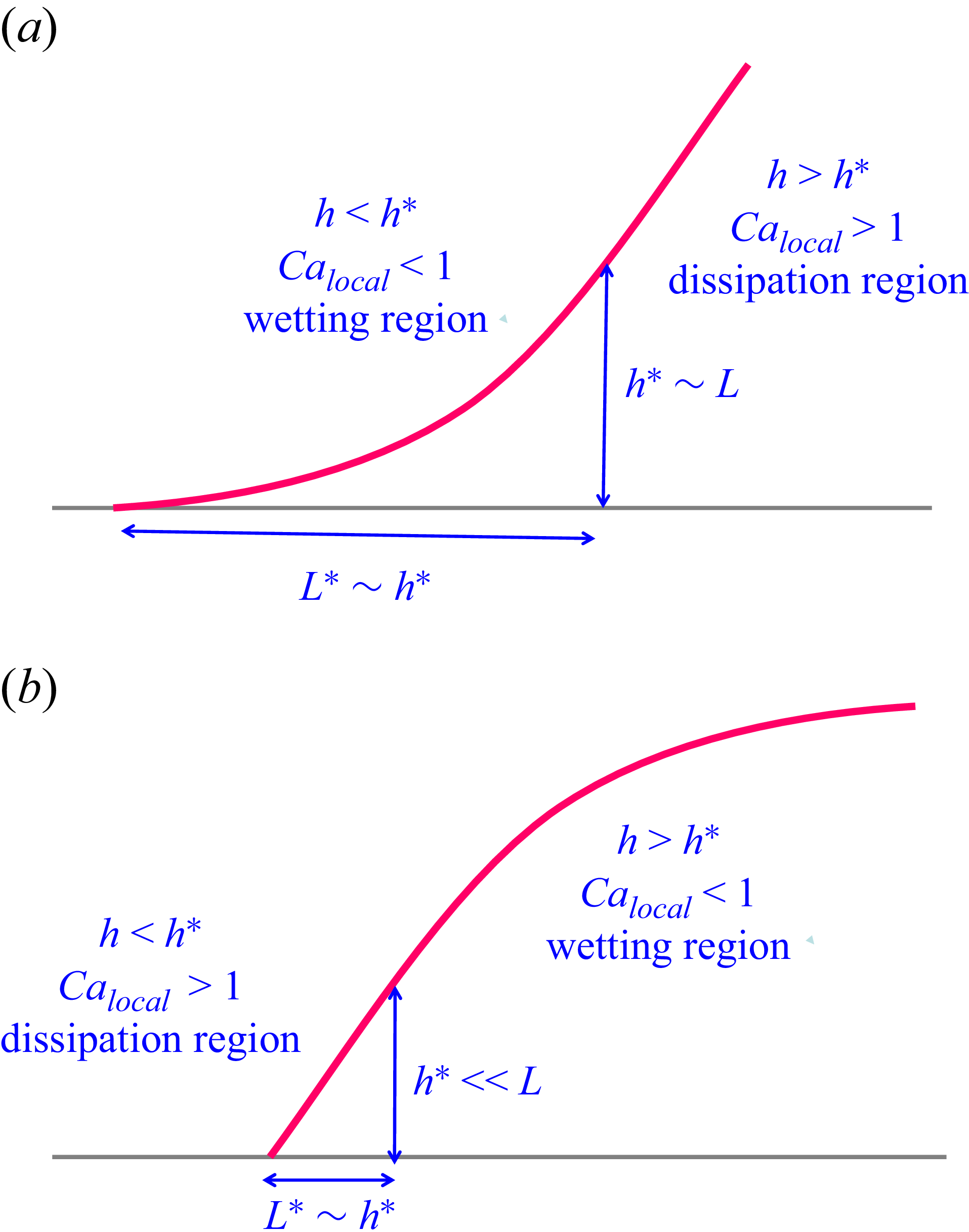
Schematic illustrations of how the characteristic dissipation length
 $ h^{*} $
influences the contact line structures for (a) shear-thinning fluids (n < 1) with large
 $ h^{*} $
extending into the bulk, and (b) shear-thickening fluids (n > 1) with small
 $ h^{*} $
near the contact line.

For
 $ n \lt 1 $
, corresponding to shear-thinning fluids, since
 $ \text{tan}\,\theta \sim {\textit{Ca}_{\textit{local}} }^{1/3} \propto h^{(1-n)/3} $
in (4.6) together with (4.5), the interface slope increases with distance from the contact line, forming a concave profile as illustrated in figure 2(a). The wetting condition (4.7) requires
 $ h^{*} \gg h $
according to (4.5) with
 $n\lt1$
, indicating that viscous dissipation extends far beyond the immediate contact line region. Because
 $ h^{*} \propto U^{n/(n-1)} $
from (4.4),
 $ h^{*} $
diverges as U→0, suggesting that the dissipation progressively expands into the bulk as the contact line advances and its speed decreases. This outer bulk dissipation region – far away from the contact line – has h >
 $ h^{*} $
or
 $ \textit{Ca}_{\textit{local}} \gt 1 $
, yielding
 $ h \sim L $
according to (4.6) and, hence,
 $ h^{*} \sim L $
. Conversely, the inner wetting region near the contact line satisfies h <
 $ h^{*} $
or
 $ \textit{Ca}_{\textit{local}} \lt 1 $
. The lateral length scale
 $ L^{*} $
corresponding to
 $ h^{*} $
, which separates these two regions, thus occurs at h ∼
 $ h^{*} $
or
 $ \textit{Ca}_{\textit{local}} $
∼ 1, giving
 $ L^{*} \sim h^{*} $
. It should be noted that in the extreme shear-thinning limit (n → 0), (4.3) reduces to the equation governing the motion of a strongly slipping contact line (Wei et al. Reference Wei, Tsao and Chu2019), where viscous dissipation is primarily confined within a fixed region of size
 $ h^{*} $
proportional to the slip length λ. With
 $ \text{tan}\,\theta \sim \theta $
when θ is small under (4.6) and (4.7), the dynamic contact angle is
 \begin{align} \theta_{d}\sim (h/h^{*})^{(1-n)/3}, \end{align}
which is consistent with (3.11b
), showing that the wetting can be enhanced with
 $ \theta \rightarrow 0 $
as
 $ h \rightarrow 0 $
due to the drag reduction effect of shear thinning.
Conversely, when
 $ n \gt 1 $
for shear-thickening fluids, the situation is markedly different. In this case, the viscosity
 $\eta \sim k(U/h)^{n-1}$
increases sharply near the contact line. According to (4.6) together with (4.5),
 $ \text{tan}\,\theta \propto 1/h^{(n-1)/3} $
, so the interface slope decreases with distance from the contact line, yielding a convex profile as illustrated in figure 2(b). The wetting condition (4.7) requires that the characteristic dissipation length satisfies
 $ h^{*}\ll h $
. This implies that the viscous dissipation is highly concentrated in a narrow region very close to the contact line. Because
 $ h^{*} \propto U^{n/(n-1)} $
from (4.4),
 $ h^{*} $
decreases as U→0, indicating that the dissipation becomes increasingly localised near the contact line as the wetting progresses. When n is large, the rate of shrinkage of
 $ h^{*} $
approaches its maximum, with
 $ h^{*} \propto U $
, corresponding to extremely shear-thickening fluids (Starov et al. Reference Starov, Tyatyushkin, Velarde and Zhdanov2003).
As also illustrated in figure 2(b), the contact line behaviours in the inner and outer regions for shear-thickening fluids are markedly different from those for shear-thinning fluids. The inner region with
 $ h \lt h^{*} $
(or
 $ \textit{Ca}_{\textit{local}} \gt 1 $
) is now dominated by strong viscous dissipation and confined within the immediate vicinity of the contact line. The outer region with
 $ h\gt h^{*} $
(or
 $ \textit{Ca}_{\textit{local}} \lt 1 $
) corresponds to the wetting zone, where surface tension prevails and interface relaxation takes place. The lateral dimension associated with
 $ h^{*} $
separates these two regions and again scales as
 $ L^{*} $
∼
 $ h^{*} \ll L $
, corresponding to the location where
 $ \textit{Ca}_{\textit{local}} \sim 1 $
.
However, to determine the apparent dynamic contact angle
 $ \theta_{d}$
in the outer wetting zone with
 $ h \gt h^{*} $
, certain precautions are needed. Since (4.6) together with (4.5) indicate that θ →π/2 as
 $ h \rightarrow 0 $
, this suggests a complete suppression of wetting. In fact, under this condition, the lubrication equation (4.3) breaks down near the contact line where the interface steepens significantly due to the mounting viscous resistance caused by the more severe contact line singularity. To sustain wetting with
 $ \theta \ll 1 $
and to alleviate the interface’s steepening and resistance, a microscopic mechanism must operate at a scale h
m
, much larger than the dissipation length
 $ h^{*} $
in the vicinity of the contact line. Consequently, when wetting occurs under (4.7), a well-defined apparent dynamic contact angle can exist only if the interface satisfies
 $h^{*}/h_{m} \ll 1$
in (4.6) with (4.5) evaluated at
 $h=h_m$
, leading to
 \begin{align} \theta_{d}\sim \left(h^{*}/h_{m}\right)^{\left(n-1\right)/3}, \end{align}
which is consistent with (3.13b ).
4.3. Review of solutions to ( 4.1 ) obtained by previous studies
Regarding the actual solution to (4.1), it is worth revisiting what has been done previously. Wang et al. (Reference Wang, Lee, Peng and Lai2007a ) analysed spreading power-law fluid drops and reported that (4.1) admits an analytical solution in a simple power-law form, i.e.
 \begin{align}h=\textit{bU}^{n/(n+2)}x^{3/(n+2)},\end{align}
with
 $b \gt 0$
being the coefficient required to satisfy (4.1). A similar solution form was also identified by Carré & Eustache (Reference Carré and Eustache2000) for shear-thinning fluids (
 $n\lt 1$
). In fact, this solution was first obtained by Boatto et al. (Reference Boatto, Kadanoff and Olla1993) who investigated various classes of travelling-wave solutions of the evolution equation
 $h_{t}+(h^{n+1}h_{xxx})_{x}=0$
. However, as pointed out by Bertozzi & Pugh (Reference Bertozzi and Pugh1996), (4.10) is valid only for
 $n\lt 1$
but not for
 $n\geq 1$
. Indeed, it can be readily verified that (4.10) does not satisfy (4.1) for
 $n\gt 1$
, since the left-hand side of (4.1) remains positive while the right-hand side is negative. Moreover, even if (4.10) were assumed in this case, it would result in
 $h^{\prime}$
diverging at the contact line (
 $x=0$
), yielding an apparent contact angle
 $\theta _{d}=90^{\mathrm{o}}$
. This is clearly unphysical, as the contact line would not advance at all, not to mention that this contradicts the small-slope assumption under which (4.1) is derived.
It is worth noting that due to nonlinearity, (4.1) can exhibit a variety of solution characteristics, depending on the value of
 $n$
(Boatto et al. Reference Boatto, Kadanoff and Olla1993). While an exact solution can sometimes exist (Abdel Kader et al. Reference Abdel Kader, Abdel and Nour2013), it is often not easily converted into a form that facilitates a clear understanding of the underlying physics. Furthermore, even with a simple solution form like (4.10), it is difficult to identify how the dynamic contact angle
 $\theta _{d}=h^{\prime}$
is influenced by the length scales involved in connection to the nature of the contact line singularity. Therefore, an approximate yet more physically oriented approach is needed to solve (4.1), which is presented next.
4.4. New dynamic contact angle relationships and Cox–Voinov generalisation
Under the assumption that
 $h^{\prime}$
is small, we employ the slowly varying slope approach to solve equations (4.1) or (4.3) approximately. This approach was first introduced by Voinov (Reference Voinov1976) in his derivation of (2.3) and later extended by Snoeijer (Reference Snoeijer2006) for the large-slope scenario. The essence of this approach is that, by assuming the shape of the macroscopic wedge to vary slowly with respect to the distance to the contact line, the dynamic contact angle formula can be derived through a straightforward integration of the equation. This approach is able to recover the Cox–Voinov law (2.3) (Wei Reference Wei2018), and its validity is supported by the fact that the numerical error due to this approximation, when compared with the full formula derived by Cox (Reference Cox1986), does not exceed 1 % for
 $\theta _{d}\lt 3\pi /4$
(Voinov Reference Voinov1976; Bonn et al. Reference Bonn, Eggers, Indekeu, Meunier and Rolley2009). Moreover, the same framework has been successfully applied to model surfactant superspreaders (Wei Reference Wei2018) and to develop a theory of slipping moving contact lines (Wei et al. Reference Wei, Tsao and Chu2019), demonstrating the robustness of this approach.
In the derivation below, following the approach of Voinov (Reference Voinov1976), we use
 $h$
as the variable to integrate (4.1) under the assumption of slowly varying
 $h^{\prime}$
. We first rewrite
 $h^{\prime\prime\prime}=h^{\prime}\textrm{d}h^{\prime\prime}/\textrm{d}h$
in (4.1) and integrate it along with the vanishing curvature condition (4.2). This yields
 \begin{align}h^{\prime\prime}=-\textit{KU}^{n}\int _{h_{ \infty }}^{h}\left(\frac{1}{h^{\prime}}\right)\,\frac{\textrm{d}x}{h^{n+1}},\end{align}
where
 $h_{ \infty }\equiv h(x\rightarrow \infty )$
. Since
 $h^{\prime}$
varies slowly, the integral on the right-hand side of (4.11) with
 $n\gt 0$
can be approximated as
 \begin{align}\left(\frac{1}{h^{\prime}}\right)\int _{h_{ \infty }}^{h}\frac{\textrm{d}x}{h^{n+1}}\approx -\left(\frac{1}{h^{\prime}}\right)\frac{1}{n}h^{-n},\end{align}
wherein we neglect
 $h_{ \infty }^{-n}$
in the final result because
 $h_{ \infty }\gg h$
. Substituting (4.12) into (4.11) and rewriting
 $h^{\prime\prime}=h^{\prime}\textrm{d}h^{\prime}/\textrm{d}h$
, we arrive at
 \begin{align}(h^{\prime})^{2}\frac{\textrm{d}h^{\prime}}{\textrm{d}h}=\left(\frac{K}{n}\right)U^{n}h^{-n}.\end{align}
As anticipated, for
 $n=1$
, integrating (4.13) recovers the Cox–Voinov law (2.3) for the Newtonian case. For power-law fluids with
 $n\neq 1$
, integrating (4.13) yields a new law for the apparent dynamic contact angle
 $\theta _{d}\equiv h^{\prime}(x)$
at
 $x\gg x_{m}$
:
 \begin{align}(h^{\prime})^{3}=\left({h_m}^{\prime}\right)^{3}+\left[\frac{3K}{n(1-n)}\right]U^{n}\left[h^{1-n}-h_{m}^{1-n}\right]\!,\end{align}
where
 $h_{m}$
(
 $\ll h)$
and
 ${h_m}^{\prime}$
(
 $\ll h^{\prime}$
) are evaluated at a mesoscopic length
 $x_{m}$
.
As indicated by (4.14), the behaviour of
 $h^{\prime}$
can be dominated by either the macroscopic
 $h^{1-n}$
term or the mesoscopic
 $h_{m}^{1-n}$
term, depending on whether
 $n\lt 1$
or
 $n\gt 1$
. These macroscopic and mesoscopic terms correspond to distinct dissipation length scales
 $L$
and
 $x_{m}$
for
 $n\lt 1$
and
 $n\gt 1$
, respectively, as also described by the braking force behaviour in (3.3).
4.4.1. The shear-thinning case
For shear-thinning fluids (n < 1), (4.14) is dominated by the
 $h^{1-n}$
term. By neglecting the contributions from
 $h_{m}$
, (4.14) reduces to
 \begin{align}(h^{\prime})^{3}=c \textit{KU}^{n}h^{1-n},\end{align}
where
 $ c = 3/n(1-n) $
. This confirms the scaling result (3.11b
). When expressed in terms of the dissipation length
 $ h^{*} $
= (KU
n
)1/(n−1) given by (4.4), (4.15) reduces to the familiar Cox–Voinov form, written in terms of the local capillary number defined by (4.5), consistent with (4.8):
 \begin{align}(h^{\prime})^{3}= c \textit{Ca}_{\textit{local}} = c (h / h^{*})^{1-n} .\end{align}
The corresponding interface profile is then
 \begin{align} h=\left[\frac{n+2}{3}\left(\textit{cK}\right)^{1/3}\right]^{3/\left(n+2\right)}U^{n/\left(n+2\right)} x^{3/\left(n+2\right)}, \end{align}
which recovers the exact solution reported previously (Boatto et al. Reference Boatto, Kadanoff and Olla1993; Carré & Eustache Reference Carré and Eustache2000; Wang et al. Reference Wang, Lee, Peng and Lai2007a
). Re-expressing (4.15) in terms of x using (4.17), we find that the apparent dynamic contact angle
 $\theta _{d}\equiv h^{\prime}(x)$
varies as
 \begin{align}\theta _{d}(x)=C_{1}U^{n/(n+2)}x^{(1-n)/(n+2)},\end{align}
where C
1 = [(n + 2)/3](1−n)/(n + 2) (cK)1/(n + 2). Note that the above results hold only for
 $x$
sufficiently far from the microscopic position
 $x_{m}$
, as the contributions from
 $h_{m}$
at that position are neglected in (4.14). Suppose that
 $\theta _{d}$
is evaluated at a fixed relative position
 $r=R-x=(1-\alpha )R$
with respect to the spreading radius
 $R$
with
 $\alpha$
being a constant (
 $\lt 1$
). Then,
 $\theta _{d}$
described by (4.18) not only varies with the extent of the spreading but also is constrained by the drop volume
 $V=(\pi /4)R^{3}\theta _{d}$
. Substitution of
 $x=\alpha R$
and
 $R=(4V/\pi \theta _{d})^{1/3}$
into (4.18) leads
 $\theta _{d}$
to vary with
 $U$
as
 \begin{align} \theta _{d}=\left[\left(\frac{4V\alpha ^{3}}{\pi }\right)^{1-n}C_{1}^{3\left(n+2\right)}\right]^{1/\left(2n+7\right)}U^{3n/\left(2n+7\right)} . \end{align}
Equation (4.19) is consistent with the
 $ \theta_{d}$
-U relationship obtained by Starov et al. (Reference Starov, Tyatyushkin, Velarde and Zhdanov2003) using self-similar analysis. In their work, the spreading law R(t) was derived first by solving the full lubrication equation across the entire drop, and the spreading speed U was subsequently expressed in term of
 $ \theta_{d}$
via the constant drop volume constraint. In contrast, the present derivation of (4.19) is achieved by resolving the local contact line behaviour directly. Furthermore, unlike the Newtonian case where the
 $ \theta_{d}$
-U relationship is independent of the drop volume V, as indicated by the Cox–Voinov law (2.3), (4.19) exhibits an explicit dependence on V, as also noted by Starov et al. (Reference Starov, Tyatyushkin, Velarde and Zhdanov2003). This arises because the dissipation length
 $ h^{*} $
given by (4.4) now extends across the entire drop body, i.e.
 $ h^{*} $
∼R. For this reason, the actual value of α– which quantifies the extent of dissipation – must be determined by solving the full equation governing the interfacial evolution of a spreading drop, as carried out by Starov et al. (Reference Starov, Tyatyushkin, Velarde and Zhdanov2003).
Writing
 $U\sim R/t$
and using
 $R^{3}\theta _{d}=$
constant again, we can use (4.19) to determine how
 $\theta _{d}$
and
 $R$
vary with time
 $t$
:
 \begin{align}\theta _{d}\propto t^{-3n/(3n+7)}, \\[-28pt] \nonumber\end{align}
 \begin{align}R\propto t^{n/(3n+7)}. \\[-2pt] \nonumber\end{align}
Equation (4.20b ) reproduces the spreading law derived by Starov et al. (Reference Starov, Tyatyushkin, Velarde and Zhdanov2003) and Betelu & Fontelos (Reference Betelu and Fontelos2004) with complete prefactors using self-similar analysis and is also consistent with the solution form proposed by King (Reference King2001). Furthermore, (4.20a ) for the dynamic contact angle evolution agrees with that derived by Betelu & Fontelos (Reference Betelu and Fontelos2004). This consistency confirms that the present formulation – based on the original contact angle relation (4.15) derived directly from the governing equation (4.1) under the volume constraint – faithfully reproduces the spreading dynamics for shear-thinning fluids. While (4.20a ) and (4.20b ) naturally arise from the self-similar analysis, our formulation underscores that these power-law dependences are not merely mathematical consequences but are intrinsically governed by the local dynamic contact angle behaviour encapsulated in (4.15). This also reinforces that the dynamic contact angle (4.15) serves a more fundamental description from which macroscopic spreading laws emerge.
In the strong shear-thinning
 $n\rightarrow 0$
limit, the approximation used in (4.12) for the right-hand side of (4.1) is no longer valid, and thus, the preceding results do not apply. In this limit, (4.1) simplifies to
 \begin{align}h^{\prime \prime \prime}=-\frac{K_{0}}{h} .\end{align}
Here
 $K_{0}=k/\gamma$
and its inverse is precisely the dissipation length described by (4.4). The same equation form also describes the motion of a strongly slipping contact line with
 $K_{0}$
being inversely proportional to the slip length (Wei et al. Reference Wei, Tsao and Chu2019). Following a similar approach as in (4.11) and (4.12), the dynamic contact angle relationship is found to be
 \begin{align}(h^{\prime})^{3}=3K_{0}h \ln (h_{ \infty }/h).\end{align}
So (
 $h^{\prime})^{3}$
is roughly proportional to
 $h$
, similar to (4.15) with small
 $n$
, albeit it weakly depends on the macroscopic height
 $h_{ \infty }$
through the logarithmic term. The corresponding interface profile is
 \begin{align}h\approx \left(3/2\right)^{3/2}\left[3K_{0}\ln (h_{ \infty }/h)\right]^{1/2}x^{3/2},\end{align}
which approximately follows
 $x^{3/2}$
, resembling (4.17) when
 $n$
is small. Both (4.22) and (4.23) have also been observed in strongly slipping moving contact lines (Wei et al. Reference Wei, Tsao and Chu2019). These results indicate that the contact line behaviour in the strong shear-thinning
 $n\rightarrow 0$
limit resembles that in the strong slip limit because of strong drag reduction due to a substantial decrease in the viscosity.
It should also be noted that the viscosity
 $\eta$
of a shear-thinning fluid does not necessarily vanish as the shear rate
 $\dot{s}$
increases indefinitely, as suggested by (3.1), especially near the contact line. Instead,
 $\eta$
may approach a finite constant value, known as the infinite-shear viscosity
 $\eta _{ \infty }$
, as
 $\dot{s}$
→ ∞, as described by the Carreau model (Bird, Armstrong & Hassager et al. Reference Bird, Armstrong and Hassager1987; Carreau, Kee & Daroux Reference Carreau, Kee and Daroux1979). In this case, the contact line structure can be conceptually divided into three subregions: an inner Newtonian-like region characterised by viscosity
 $\eta _{ \infty }$
, an outer region exhibiting shear-thinning behaviour with a higher apparent viscosity and an intermediate transition region connecting the two (Charitatos et al. Reference Charitatos, Suszynski, Carvalho and Kumar2020).
In fact, the behaviour of such Carreau shear-thinning fluids is somewhat similar to polymeric liquids where viscosity is significantly reduced near a substrate due to the depletion layer (De Gennes Reference de Gennes1985). This results in an apparent slip length
 $\lambda$
near the contact line where viscosity decreases from the bulk value η
b
to
 $\eta_{\infty}$
. As the shear stress near the contact line behaves as
 \begin{align}\tau =\eta \frac{\partial u}{\partial y}\sim \eta _{b}\frac{U}{h+\lambda }\sim \eta _{ \infty }\frac{U}{h} ,\end{align}
the slip length λ can be related to the viscosity reduction ratio through
 \begin{align}\frac{\lambda }{h}\sim \frac{\eta _{b}}{\eta _{ \infty }}-1,\end{align}
establishing a connection between shear-thinning effects and slip effects. When this viscosity-reduction-induced slip effect becomes pronounced, i.e.
 $ \lambda/h \gg 1$
, the apparent dynamic contact angle can be shown to behave as
 $ \theta_{d}$
∼ Ca
b
1/2 in terms of the capillary number
 $ \textit{Ca}_{b} = \eta_{b} U/\gamma $
based on the bulk viscosityη
b
(Wei et al. Reference Wei, Tsao and Chu2019). This scaling deviates significantly from the classical Cox–Voinov law
 $ \theta_{d}$
∼ Ca
b
1/3 given by (2.3). Recently, Yancheshme et al. (Reference Yancheshme, Yoon, Palmese and Alvarez2024) performed drop spreading experiments for a variety of shear-thinning fluids and found that the measured dynamic contact angles approximately collapse according to
 $ \theta_{d}$
∼ Ca
b
0.51. The excellent agreement with this prediction strongly supports the notion that shear-induced viscosity reduction near the contact line effectively enhances slip, thereby altering the local dissipation mechanism and leading to a stronger dependence of the dynamic contact angle on the capillary number.
Another aspect worth noting is that as the shear rate
 $\dot{s}$
→ 0, the viscosity η should asymptotically approach the zero-shear viscosity η
0, which corresponds to the bulk viscosity η
b
mentioned above and cannot be captured by the simple power-law model (3.1). It might happen that in the outer region sufficiently far away from the contact line, the local shear rate becomes very small, η is therefore dominated by the zero-shear viscosity plateau η
0. This might accompany the inner contact line region where
 $\dot{s}$
is large but not yet high enough to reach the infinite-shear viscosity plateau
 $\eta_{\infty}$
, its viscosity may still follow the power-law dependence described by (3.1). Under such circumstances, η can be more accurately represented by the Ellis model, which incorporates only a zero-shear viscosity plateau, or by the Carreau model, which accounts for both the zero-shear and infinite-shear viscosity plateaus (Bird et al. Reference Bird, Armstrong and Hassager1987). In either model, the transition from the outer Newtonian (low
 $\dot{s}$
) regime to the inner shear-thinning (high
 $\dot{s}$
) regime occurs at a critical shear rate,
 $\dot{s}_{c}$
, below or above which the contact line behaviour is respectively Newtonian or shear-thinning. This also defines the corresponding critical liquid height
 $ h_{c} \sim U/\dot{s}_{c} $
below or above which the contact line dynamics exhibit shear-thinning or Newtonian characteristics. When
 $\dot{s}_{c}$
is large, h
c
becomes small and, thus, is easily exceeded, making the contact line behaviour predominantly Newtonian. This height may effectively act as a velocity-dependent slip length λ to alleviate the contact stress singularity in Newtonian fluids. In that case, the apparent dynamic angle can be described by the classical Cox–Voinov law with
 $\ell = 0.54 \lambda \textit{Ca}^{-1/3}$
in (2.3) (Eggers & Stone Reference Eggers and Stone2004), where
 $ \textit{Ca} = \eta_{0} U/\gamma $
is the capillary number based on the zero-shear viscosity η
0. When
 $\dot{s}_{c}$
is small, however, the contact line region becomes shear thinning and the local viscosity decreases markedly with increasing shear rate. In this regime, an effectively large slip length may emerge due to the substantial viscosity reduction according to (4.25). This in turn results in a weak stress singularity, making the dynamic contact angle deviated from the classical Cox–Voinov law as indicted by (4.19).
4.4.2. The shear-thickening case
For shear-thickening fluids with
 $n\gt 1$
, we rewrite (4.14) in terms of the characteristic dissipation length
 $h^{*}$
defined by (4.4),
 \begin{align}(h^{\prime})^{3}=(h_{m}')^{3}+c\left[\left(\frac{h^{*}}{h_{m}}\right)^{n-1}-\left(\frac{h^{*}}{h}\right)^{n-1}\right]\! ,\end{align}
with
 $ c = 3/n (n-1)$
. Equation (4.26) shows that the slope
 $h^{\prime}(x)$
increases monotonically with
 $h$
as
 $h$
grows toward the bulk. As
 $h\rightarrow \infty $
when
 $x\rightarrow \infty $
,
 $h'$
approaches a constant value, representing the apparent dynamic contact angle
 $\theta _{d}\equiv \tan ^{-1}(h^{\prime}(x\rightarrow \infty ))$
, leading (4.26) (neglecting
 $(h_{m}^{\prime})^{3}$
) to
 \begin{align} {\theta_{d}}^{3}=cCa_{\textit{local}}\left(h_{m}\right)= (h^{*}/ h_{m})^{n-1}, \end{align}
which is essentially (4.9) with the local capillary number
 $ \textit{Ca}_{\textit{local}} $
evaluated at h = h
m
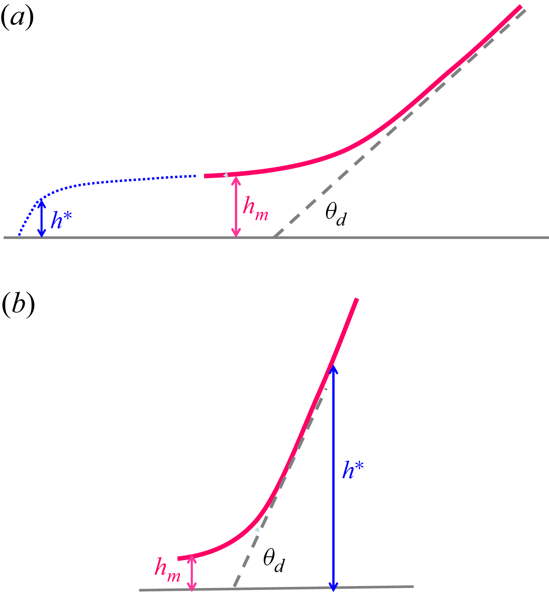
. Equation (4.27) indicates that wetting under small values of
 $\theta _{d}$
would become more favourable when
 $h^{*}\lt h_{m}$
(see figure 3
a). Since
 $h^{*}=(\textit{KU}^{n})^{1/(n-1)}$
according to (4.4), this implies that favourable wetting can only be achieved when the speed
 $U$
is below a certain critical value,
 $U_{c}$
:
Schematic illustrations showing how the contact line structure for shear-thickening fluids (
 $n\gt 1$
) is influenced by the relative size of the dissipation length
 $h^{*}$
compared with the microscopic cutoff
 $h_{m}$
. Results are shown for (a)
 $h^{*}\ll h_{m}$
and (b)
 $h_{m}\ll h^{*}$
.

 \begin{align}U_{c}=\big(K^{-1}h_{m}^{n-1}\big)^{1/n}.\end{align}
In this case, the apparent dynamic angle is
 \begin{align}\theta _{d} \approx C_{2}\left(\frac{k}{\gamma }\right)^{1/3}U^{n/3}h_{m}^{(1-n)/3},\end{align}
which is (3.13b ), where C 2 = (c(2 + 1/n) n )1/3. The apparent dynamic contact relationship (4.29) is new and stands in contrast to that proposed by Wang et al. (Reference Wang, Lee, Peng and Lai2007a ), where the same functional form derived for shear-thinning fluids was applied to shear-thickening fluids.
On the other hand, if
 $U\gt U_{c}$
, this means
 $h^{*}\gt h_{m}$
, which may cause the dynamic contact angle
 $\theta _{d}$
to no longer be small and even approach
 $90^{\circ}$
(see figure 3b
). In this case, wetting becomes less favourable. Note from (4.26) that
 $h^{\prime}(x)$
will be smaller than
 $h_{m}^{\prime}\equiv h^{\prime}(x_{m})$
when
 $h\lt h_{m}$
and continue to decrease as
 $h$
approaches the contact line. If there is a pre-wetted film ahead of the macroscopic contact line, this will allow
 $h^{\prime}(x)$
to continuously decrease towards zero, with
 $h^{\prime}=0$
at some
 $h\lt h_{m}$
or
 $x\lt x_{m}$
. Since
 $h^{\prime}$
cannot be further decreased to a negative value below this point, an additional mechanism is required to ensure that this zero-slope location also acts as an inflection point
 $h^{\prime\prime}=0$
. Below this point,
 $h^{\prime}$
must necessarily increase as it moves towards the microscopic contact line. Given that
 $h$
is very small in this region, this inflection point and subsequent film thinning below it can only arise from disjoining pressure effects. For the potentially large
 $\theta _{d}$
situation when
 $h^{*}\gt h_{m}$
, the presence of a precursor film due to disjoining pressure would become even more essential to facilitate the forward movement of the contact line. In any case, the thickness of the precursor film, which determines
 $h_{m}$
, and the extent of its spread will be governed by the detailed profile of the film, which is examined in § 5.
4.5. Summary and comparison with literature
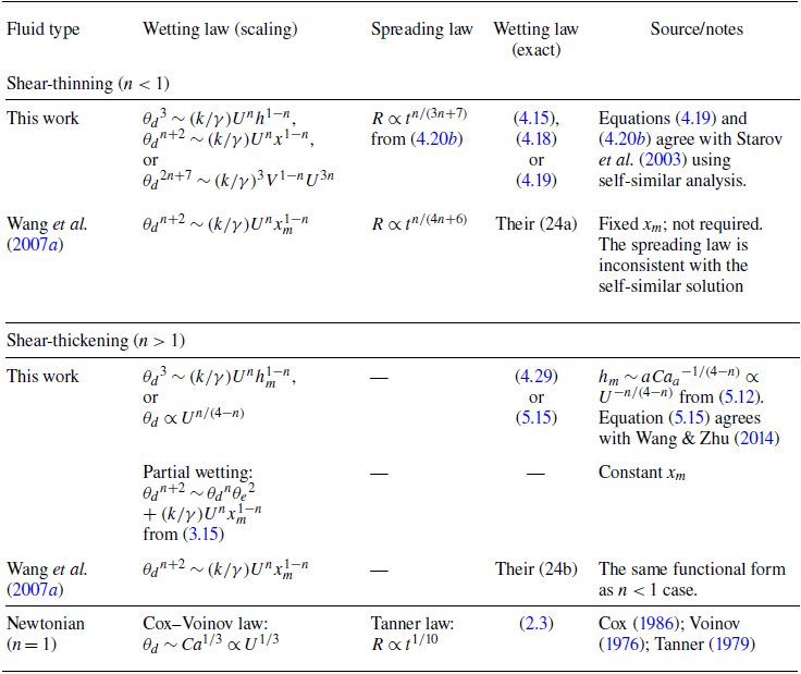
Having completed the derivations of the apparent dynamic contact angle relationships for both shear-thinning and shear-thickening fluids in §§ 4.4.1 and 4.4.2, table 1 summarises these results and the corresponding spreading laws in comparison with those reported by previous work.
Summary of theoretical predictions for dynamic contact angle relationship (called wetting law) and spreading law in power-law fluids.

For shear-thinning fluids (n < 1), how the dynamic contact angle
 $ \theta_{d}$
varies with the contact line speed U is found to be size dependent, described by
 $ {\theta_{d}}^{3} \sim (k/ \gamma)U^{n}h^{1-n} $
from (4.15) or
 $ {\theta_{d}}^{n+2} \sim (k/\gamma)U^{n}x^{1-n}$
from (4.18). The resulting wetting law and spreading law are
 $ \theta_{d} \propto U^{3n/(2n+7)}$
from (4.19) and
 $ R \propto t^{n/(3n + 7)}$
in (4.20b
), recovering the results of Starov et al. (Reference Starov, Tyatyushkin, Velarde and Zhdanov2003) using self-similar analysis. This consistency also validates our contact-line-based approach. In difference, Wang et al. (Reference Wang, Lee, Peng and Lai2007a
) obtained
 ${\theta_{d}}^{n+2} \sim (k/ \gamma)U^{n}{x_{m}}^{1-n}$
with a fixed microscopic cutoff
 $x_{m}$
that is not required. This yields
 $ R \propto t^{n/(4n+6)} $
– a result inconsistent with the self-similar solution.
For shear-thickening fluids (n > 1) under complete wetting conditions, our analysis shows
 $ {\theta_{d}}^{3} \sim (k/ \gamma)U^{n}{h_{m}}^{1-n} $
from (4.29) with a required microscopic h
m
. As shown later in § 5, if h
m
is provided by the microscopic precursor film induced by disjoining pressure, it can vary with the contact line speed U as
 $ h_{m} \propto U^{-n/(4 - n)} $
, leading to
 $\theta _{d} \propto U^{n/(4-n)}$
reported previously by Wang & Zhu (Reference Wang and Zhu2014). For partial wetting where the required microscopic cutoff
 $x_{m}$
becomes a fixed quantity depending on the substrate’s wettability, the dynamic contact angle relationship is modified to
 $ {\theta_{d}}^{n+2} \sim {\theta_{d}}^{n} {\theta_{e}}^{2} + (k/\gamma) U^{n}x_{m}^{1-n}$
from (3.15). For Newtonian fluids (n = 1), the theory reduces to the classical Cox–Voinov law
 $ {\theta_{d}} \sim \textit{Ca} ^{1/3} \propto U^{1/3} $
given by (2.3) and to Tanner’s spreading law
 $ R \propto t^{1/10} $
.
5. Precursor film theory for power-law fluids
In this section we examine the microstructure of the contact line in power-law fluids, with particular emphasis on shear-thickening fluids. In such fluids, the stress singularity at the contact line is more severe and, therefore, necessitates the introduction of a microscopic cutoff for regularisation. We focus on the microstructure induced by a precursor film that extends ahead of the macroscopic contact line. This film typically has a thickness of 10–100 nm (Kavehpour, Ovryn & McKinley Reference Kavehpour, Ovryn and McKinley2003) and often forms due to van der Waals disjoining pressure (Bonn et al. Reference Bonn, Eggers, Indekeu, Meunier and Rolley2009):
 \begin{align}\Pi =\gamma \frac{a^{2}}{h^{3}}.\end{align}
Here
 $a=(A/6\pi \gamma )^{1/2}$
is the molecular length, which is typically an order of 0.1 nm, and
 $A$
is the Hamaker constant.
The equation governing the precursor film motion can be derived by adding the disjoining pressure term
 $-\Pi$
from (5.1) to the capillary pressure
 $-\gamma h^{\prime\prime}$
, modifying (4.1) to
 \begin{align}h^{\prime \prime \prime}=-K\frac{U^{n}}{h^{n+1}}+\frac{3a^{2}h^{\prime}}{h^{4}}.\end{align}
We first determine the scales for the precursor film thickness
 $h_{\!f}$
and its lateral extent
 $\ell$
f
by balancing the terms in (5.2). This can be more conveniently done by rewriting (5.2) into the form analogous to the Newtonian case, i.e.
 \begin{align}h^{\prime \prime \prime}=-\frac{\mathcal{C}}{h^{2}}+\frac{3a^{2}h^{\prime}}{h^{4}},\end{align}
where
 $\mathcal{C}=\textit{KU}^{n}/h^{n-1}$
represents the effective capillary number that varies with h. This quantity is essentially the local capillary number defined by (4.5), evaluated within the microscopic precursor film region. We begin with
 $h_{\!f}^3\sim \mathcal{C}\ell_{f}^{3}$
by balancing the surface tension term
 $h^{\prime\prime\prime}\sim h_{\!f}/\ell_{f}^{3}$
with the viscous term
 $\mathcal{C}/h^{2}\sim \mathcal{C}/h_{\!f}^{2}$
. Similarly, balancing the disjoining pressure term
 $3a^{2}h^{\prime}/h^{4}\sim a^{2}\ell_{f}^{-1}/h_{\!f}^{3}$
with the surface tension term
 $h_{\!f}/\ell_{f}^{3}$
yields
 $h_{\!f}^{2}\sim a\ell_{f}$
. Combining these two relations, we obtain
 $h_{\!f}$
and
 $\ell_{f}$
in terms of
 $\mathcal{C}$
(Bonn et al. Reference Bonn, Eggers, Indekeu, Meunier and Rolley2009):
 \begin{align}h_{\!f}\sim a\mathcal{C}^{-\frac{1}{3}},\quad \ell_{f}\sim a\mathcal{C}^{-\frac{2}{3}}.\end{align}
Because
 $\mathcal{C}$
involves h ∼ h
f
we wish to determine, we rewrite it as
 $\mathcal{C}=Ca_{a}(a/h)^{n-1}$
in terms of the molecular capillary number Ca
a
 $=\textit{KU}^{n}/a^{n-1}$
. With this,
 $h_{\!f}$
and
 $\ell_{f}$
in (5.4) can be determined as
 \begin{align}h_{\!f}\sim aCa_{a}^{-\frac{1}{4-n}},\qquad\ell_{f}\sim aCa_{a}^{-\frac{2}{4-n}}.\end{align}
To solve for the film profile governed by (5.2), we non-dimensionalise (5.2) using
 $\phi =h/h_{\!f}$
and
 $\zeta =x/\ell_{f}$
based on (5.5), i.e.
 \begin{align}\phi ^{\prime \prime \prime}=-\frac{1}{\phi ^{n+1}}+\frac{3\phi^{\prime}}{\phi ^{4}},\end{align}
where primes denote derivatives with respect to
 $\zeta$
. For numerical calculations, it is more convenient to utilise the asymptotic solution
 $\phi _{- \infty }$
as
 $\zeta \rightarrow - \infty $
, away from the macroscopic contact line. This solution is obtained by balancing the driving viscous
 $\phi ^{-(n+1)}$
term with the disjoining pressure term
 $3\phi^{\prime}/\phi ^{4}$
, since the film profile in this region is nearly flat (except near the tip) and the surface tension
 $\phi ^{\prime\prime\prime}$
term can be considered small compared with the other two terms. This yields
 \begin{align}\phi _{- \infty }=\left(\frac{3}{(2-n)(-\zeta )}\right)^{\frac{1}{2-n}}\!.\end{align}
The correction to the asymptotic solution (5.7) due to surface tension, denoted as
 $\psi$
, is a static adjustment. It is obtained by balancing the perturbed disjoining pressure term
 $3\psi^{\prime}/\phi _{- \infty }^{4}$
with the surface tension term
 $\psi ^{\prime\prime\prime}$
:
 \begin{align}\psi ^{\prime \prime \prime}=\frac{3\psi^{\prime}}{\phi _{- \infty }^{4}}.\end{align}
Following Hervet & De Gennes (Reference Hervet and de Gennes1984) and Eggers & Stone (Reference Eggers and Stone2004), the approximate solution to (5.8) can be determined as follows using the Wentzel–Kramers–Brillouin (WKB) method (see Appendix C for detailed derivation):
 \begin{align}\psi =g_{0}^{-3/2}\exp \left(\int\! g_{0}\textrm{d}\zeta \right)\!,\end{align}
where
 \begin{align}g_{0}=\frac{\sqrt{3}}{\phi _{- \infty }^{2}}.\end{align}
The more accurate asymptotic film profile can therefore be constructed by adding
 $\psi$
described by (5.9) to
 $\phi _{- \infty }$
described by (5.7), i.e.
 \begin{align}\phi =\phi _{- \infty }+\Lambda \psi ,\end{align}
with
 $\Lambda$
being the adjustable coefficient. For a given value of
 $\Lambda$
, we use (5.11) to specify the values of
 $\phi$
,
 $\phi^{\prime}$
and
 $\phi ^{\prime\prime}$
at
 $\zeta =\zeta _{0}\lt 0$
, which serve as the initial conditions to integrate (5.6) numerically towards
 $\zeta \gt 0$
. The values of
 $\Lambda$
and
 $\zeta _{0}$
are selected such that the solution asymptotically satisfies the zero-curvature condition at infinity,
 $\phi ^{\prime\prime}(\zeta \rightarrow \infty )\rightarrow 0$
. For a given value of
 $n$
, we find that the value of
 $\Lambda$
is not too sensitive to the choice of
 $\zeta _{0}$
as long as
 $|\zeta _{0}|$
is sufficiently large. For
 $n=$
1.1, 1.2,1.3 and 1.4, the respective values of
 $\Lambda$
are 3.407, 1.442, 0.512 and 0.073.
Computed interface profiles (red solid lines) from numerical integration of (5.6) for shear-thickening fluids at different values of
 $n\gt 1$
. The results perfectly match the corresponding profiles (black dotted lines) in the outer wedge (macroscopic contact angle) region according to (4.29). Here Ca
a
 $=\textit{KU}^{n}/a^{n-1}=0.1$
.

Figure 4 displays the computed interface profiles for these
 $n$
values (scaled by the molecular length
 $a$
) with the cutoff
 $h_{m}$
taken as the computed interface height at
 $x=0$
. These profiles exhibit excellent agreement with the asymptotic wedge profiles corresponding to the apparent contact angle given in (4.29). This result confirms the scaling relation (5.5a
) for the film thickness, indicating that the cutoff takes the form
 \begin{align} {h_m} = \chi aC{a_a}^{ - 1/(4 - n)} \propto {U^{ - n/(4 - n)}},\end{align}
where χ is a numerical factor determined by matching the macroscopic contact line, depending on the value of
 $ n(\gt 1) $
.
We now revisit the relationship (4.27) for the apparent dynamic contact angle
 $\theta _{d}$
in terms of Ca
a
 $=\textit{KU}^{n}/a^{n-1}$
, i.e.
 \begin{align} {\theta _d} \equiv h^{\prime}(x \to \infty ) = c^{\prime}{\left( {\frac{{{h^*}}}{{{h_m}}}} \right)^{(n - 1)/3}} = c^{\prime}{\left( {\frac{{{a}}}{{{h_m}}}} \right)^{(n - 1)/3}}C{a_a}^{1/3},\end{align}
with
 $ c^{\prime} = [3/n(n-1)]^{1/3} $
. Note that in (5.13), the molecular capillary number Ca
a
can be rewritten as
 \begin{align}Ca_{a}=\eta _{a}\frac{U }{\gamma },\end{align}
based on the viscosity over the molecular length
 $a$
,
 \begin{align}\eta _{a}=\big(2+n^{-1}\big)^{n}k\left(\frac{U}{a}\right)^{n-1}.\end{align}
Substituting (5.12) for
 $h_{m}$
into (5.13) gives
 \begin{align} \theta _{d}= c^{\prime}\chi ^{-\left(n-1\right)/3}Ca_{a}^{1/\left(4-n\right)} \propto U^{n/\left(4-n\right)} , \end{align}
which is consistent with the scaling result reported by Wang & Zhu (Reference Wang and Zhu2014), but here the exact coefficient is explicitly provided.
To facilitate the interpretation of (5.15), we rewrite Ca
a
in (5.15) as
 $ \textit{Ca}_{a} = \textit{Ca}_{\textit{eff}} (h_{m}/a)^{n-1} $
in terms of the effective capillary number,
 \begin{align}Ca_{\mathit{eff}}=\eta_{\kern-1.5pt f}\frac{U}{\gamma } ,\end{align}
based on the viscosity
 $\eta_{\kern-1.5pt f}$
over the microscopic cutoff film thickness
 $h_{m}$
:
 \begin{align} \eta_f= \big(2+n^{-1} \big)^nk\left(\frac{U}{h_{m}}\right)^{n-1} . \end{align}
The microscopic viscosity defined above is experimentally identifiable, as the microscopic cutoff h m can be taken as the precursor film thickness – typically of the order of 10–100 nm. This thickness can be measured using optical techniques. Optical interferometry (Kavehpour et al. Reference Kavehpour, Ovryn and McKinley2003; Hoang & Kavehpour Reference Hoang and Kavehpour2011) is an effective technique for measuring film thicknesses in the nanometre to micrometre range near spreading contact lines. Phase-shifting imaging ellipsometry (Shoji et al. Reference Shoji, Kaneko, Yonemura, Kubo, Tsukada and Komiya2021) provides two-dimensional thickness profiles with nanometre-scale resolution, which thus enables accurate characterisation of the precursor film structure. Another approach is fluorescence microscopy (Hoang et al. Reference Hoang, Berteloot, Sharif-Kashani and Kavehpour2012) that offers a non-invasive technique capable of measuring film thicknesses from nanometres to millimetres with high resolution. The rheological parameters n and k can be measured using standard rheometric measurements. The contact line speed U, of course, is readily obtainable from experiments.
Re-expressing (5.15) in terms of Ca
eff
using
 $ (h_{m}/a)^{n-1} $
and substituting (5.12) for h
m
, (5.15) can be reduced to the familiar Cox–Voinov form:
 \begin{align} \theta_{d}=c^{\prime}C{a_{\textit{eff}}}^{1/3} . \end{align}
In fact, (5.17) is independent of specific microscopic mechanisms, as it is essentially (4.27) with the local capillary number
 $ \textit{Ca}_{\textit{local}} $
evaluated at h = h
m
representing the effective capillary number Ca
eff
. This result is significant because it elegantly extends classical theories of dynamic wetting – originally developed for Newtonian fluids – to non-Newtonian, power-law fluids, while preserving a familiar scaling structure. The key implications are as follows. First, Ca
eff
adapts the classical capillary number
 $ \textit{Ca}=\eta U/\gamma$
for non-Newtonian fluids by replacing the constant viscosity
 $\eta$
with a microscopically scaled viscosity
 $\eta_{\kern-1.5pt f}$
based on the local film thickness
 $h_{m}$
. As a result, the apparent contact angle
 $\theta _{d}$
captures this intricate interplay between shear-dependent viscosity and film thickness – revealing how microscale physics governs macroscale observables. More importantly, this reformulation leads to a universal scaling law (5.17) that is analogous to the Cox–Voinov law for Newtonian fluids, demonstrating that even in the presence of complex rheology, the dynamic wetting behaviour maintains a simple and interpretable structure.
6. Comparison with experiments
Having established a comprehensive theoretical framework, we now compare our predictions with experimental observations. Figure 5 presents the measured dependence of the dynamic contact angle
 $\theta _{d}$
on the spreading speed
 $U$
from drop spreading experiments by Wang et al. (Reference Wang, Lee, Peng and Lai2007a
) and Carré and Eustache (Reference Carré and Eustache2000) using shear-thinning fluids (
 $n\lt 1$
). The data are presented on a log–log scale, allowing us to identify the power-law relationship
 $\theta _{d}\sim U^{m}$
from the slope
 $m$
. For the rheological exponent
 $n$
= 0.4378 and 0.79, the measured power values are
 $m$
= 0.16 and 0.26, respectively, which are in excellent agreement with the corresponding theoretical values
 $3n/(2n+7) \approx$
0.167 and 0.276, as given by (4.19). Wang et al. (Reference Wang, Lee, Peng and Lai2007a
) predicted
 $m=n/(n+2) \approx$
0.180 and 0.283 according to (4.18) with x being taken as a fixed value
 $x_{m}$
, which are slightly higher than ours.
Comparison between experimental data (symbols) and theory predictions for the measured relationship between dynamic contact angle (
 $\theta _{d}$
) and the wetting speed (U) (in log–log scale) in shear-thinning fluids (
 $n\lt 1$
). (a) In the experiment by Wang et al. (Reference Wang, Lee, Peng and Lai2007a
) with n = 0.4378, the best fit (dashed line) is
 $\theta _{d}=48.406U^{0.1576}$
, yielding the slope
 $\approx 0.16$
, in good agreement with our theoretical prediction
 $3n/(2n+7) \approx 0.17$
according to (4.19). (b) In the experiment by Carré & Eustache (Reference Carré and Eustache2000) with n = 0.79, the best fit curve (dashed line) is given by
 $\theta _{d}=412.09U^{0.2606}$
, resulting in the slope
 $\approx 0.26$
, which closely matches with our theoretical prediction
 $3n/(2n+7) \approx 0.28$
.

Although the differences are minor, we believe that our dynamic contact angle relationship (4.19) captures the underlying physics more fundamentally than Wang et al.’s (Reference Wang, Lee, Peng and Lai2007a
). This is because (4.19) is derived directly from the generalised Cox–Voinov law (4.16) through the emergence of characteristic dissipation length
 $ h^{*} $
defined by (4.4). Such a generalisation can be tested by plotting the measured dynamic contact angle
 $ \theta_{d}$
against the local capillary number
 $ \textit{Ca}_{\textit{local}} $
defined by (4.5). Using
 $ h \thickapprox \theta_{d} R$
together with
 $R = (4V/\pi \theta_{d})^{1/3}$
and substitution of (4.4) for
 $ h^{*} $
,
 $ \textit{Ca}_{\textit{local}} $
can be written as
 \begin{align} Ca_{\textit{local}}=\frac{kU^n}{\gamma }\left(2+\frac{1}{n}\right)^{n}\left(\frac{4}{\pi }V\right)^{\frac{1-n}{3}}{\theta _{d}}^{\frac{2}{3}\left(1-n\right)} , \end{align}
in terms of measurable rheological parameters k,
 $ \gamma $
and n, the drop volume V and the dynamic contact angle
 $ \theta_{d}$
. Figure 6 replots the measured values of
 $ \theta_{d}$
from figures 5(a) and 5(b) against
 $ \textit{Ca}_{\textit{local}} $
defined in (6.1). The data collapse remarkably well onto the predicted scaling
 $ \theta_{d} \sim {\textit{Ca}_{\textit{local}}}^{1/3}$
, consistent with the generalised Cox–Voinov law (4.16). This demonstrates that the dynamic contact angle is controlled by the local capillary number incorporating the characteristic dissipation length
 $ h^{*} $
, thereby validating our theoretical prediction.
Replot of the measured dynamic contact angle
 $ \theta_{d}$
from figure 5 against the local capillary number
 $ \textit{Ca}_{\textit{local}} $
defined in (6.1). The data collapse onto a single trend
 $ \theta_{d} \sim {\textit{Ca}_{\textit{local}}}^{1/3}$
according to the generalised Cox–Voinov law (4.16).

Another reason we regard the model of Wang et al. (Reference Wang, Lee, Peng and Lai2007a
) as less essential is the presence of an internal inconsistency in their derivation. Our formulation also recovers the same power expression
 $m=n/(n+2)$
from the original version of the dynamic contact angle relation (4.18), just as in Wang et al.’s formulation. However, that relation indicates that
 $\theta _{d}$
depends on the distance to the contact line x, which should actually be the order of a macroscopic length L, since viscous dissipation extends into the bulk. In drop spreading,
 $L$
is typically taken to be the drop spreading radius
 $R$
, which is not an independent variable but instead varies inversely with
 $\theta _{d}$
due to the constant drop volume constraint. Once this interdependence is properly accounted for, the resulting relationship becomes (4.19), yielding the exponent
 $m=3n/(2n+7)$
. This contrasts sharply with Wang et al. (Reference Wang, Lee, Peng and Lai2007a
), who treated
 $x$
as a fixed microscopic length
 $x_{m}$
, which appears unnecessary because the contact line force is finite as indicated by (3.6).
A comparison can also be made from the perspective of drop spreading dynamics by linking the dynamic contact angle relationship to the spreading law. Under the constant drop volume constraint
 $R^{3}\theta _{d}=$
constant again, the dynamic contact angle relationship
 $\theta _{d}\sim U^{m}\sim (R/t)^{m}$
implies a spreading law
 $R\sim t^{\nu }$
with the spreading exponent
 $\nu =m/(m+3)$
, where
 $t$
is time. Substituting
 $m=3n/(2n+7)$
from our derived
 $ \theta_{d}$
–U relationship (4.19) yields
 $\nu =n/(3n+7)$
, identical to (4.20b
) obtained from the self-similar solutions (Starov et al. Reference Starov, Tyatyushkin, Velarde and Zhdanov2003; Betelu & Fontelos Reference Betelu and Fontelos2004).
Figure 7(a) shows the plot of R vs t based on the experimental data of Rafaï et al. (Reference RafaÏ, Bonn and Boudaoud2004), from which the spreading exponent ν is obtained by fitting a power law. Figure 7(b) presents a similar plot but in log–log scale, using the data of Wang et al. (Reference Wang, Zhang, Lee and Peng2007
b), from which ν is extracted from the slopes. As summarised in figure 7(c), the measured
 $\nu$
values for various
 $n$
exhibit a reasonable agreement with the theoretical prediction
 $ \nu = n/(3n+7) $
. Although this comparison was previously reported by Wang et al. (Reference Wang, Zhang, Lee and Peng2007b
), we include it here to highlight that the spreading exponent
 $ \nu = n/(3n+7) $
directly follows the contact angle exponent
 $m = 3n/(2n+7)$
.
Plots of spreading radius,
 $R$
, versus time,
 $t$
, for shear-thinning fluids (
 $n\lt 1$
) obtained from drop spreading experiments by (a) Rafaï et al. (Reference RafaÏ, Bonn and Boudaoud2004) and (b) Wang et al. (Reference Wang, Zhang, Lee and Peng2007b
). Solid lines represent best fits using R = Γ t
ν to determine the spreading exponent
 $\nu$
. (c) Comparison between experiment and theory: plot of
 $\nu$
versus the rheology exponent
 $n$
. The trend of the measured
 $\nu$
values from (a) and (b) is reasonably captured by the theoretical prediction
 $ \nu = n/(3n+7) $
.

It is also worth noting that the alternative expression
 $\nu =n/(4n+6)$
derived from
 $m=n/(n+2)$
as based on Wang et al. (Reference Wang, Lee, Peng and Lai2007a
) also reproduces experimental trends reasonably well, although their formulation is not consistent with the self-similar solution. The discrepancy arises because, in their analysis, the microscopic lateral length scale
 $x_{m}$
– which is not required in the present work – is treated to be a constant, for example, through the introduction of a slip length. Such a situation cannot be entirely ruled out, since a substantial reduction in the fluid viscosity near the contact line could generate a depletion-layer-like effect and thereby a large apparent slip length, as indicated by (4.25). Since their exponent
 $m=n/(n+2)$
and our exponent
 $m=3n/(2n+7)$
are not very distinguishable over the experimentally relevant range of n (typically 0.5–1), both formulations predict similar spreading exponents ν and, thus, comparable macroscopic behaviours. This explains why the experimental data of Wang et al. (Reference Wang, Lee, Peng and Lai2007a
) appear to agree reasonably well with both models, despite distinct theoretical foundations between their and our models. Determining which formulation more faithfully captures the true physics likely requires investigations at the microscopic level.
It is also possible that there exists a microscopic structure ahead of the macroscopic contact line, even though no microscopic cutoff is required in shear-thinning fluids. Consequently, beyond our model and that of Wang et al. (Reference Wang, Lee, Peng and Lai2007a
), other formulations may likewise reproduce the observed trends in the dynamic contact angle. Identifying which model truly reflects the underlying contact line physics ultimately hinges on characterising the microstructure – arising from a molecular-force-driven precursor film, slip or the equilibrium contact angle – located ahead of the macroscopic contact line (Wei et al. Reference Wei, Tsao and Chu2019; Chan et al. Reference Chan, kamal, snoeijer, spritles and eggers2020). In particular, if a precursor film is present, its microscopic thickness h
m
and lateral extent
 $x_{m}$
will generally depend on the contact line speed U, which in turn can fundamentally alter the dependence of the spreading exponent m on n, producing behaviours that differ from both our prediction and that of Wang et al. (Reference Wang, Lee, Peng and Lai2007a
). In any case, h
m
and
 $x_{m}$
, if they exist, may be inferred from a modelled dynamic contact angle relationship
 $\theta _{d}$
(U) or measured directly using optical techniques (Kavehpour et al. Reference Kavehpour, Ovryn and McKinley2003; Hoang & Kavehpour Reference Hoang and Kavehpour2011; Hoang et al. Reference Hoang, Berteloot, Sharif-Kashani and Kavehpour2012; Shoji et al. Reference Shoji, Kaneko, Yonemura, Kubo, Tsukada and Komiya2021).
It should be noted that, in the above comparison for shear-thinning fluids, the prefactors in the power-law relationships
 $\theta _{d}\sim U^{m}$
and
 $R\sim t^{\nu }$
represent the geometrical shape factors of the spreading drop. These factors generally depend on the overall drop geometry and its dimensions, as reflected in the self-similar solutions (Starov et al. Reference Starov, Tyatyushkin, Velarde and Zhdanov2003; Betelu & Fontelos Reference Betelu and Fontelos2004). In practice, however, the drop may deviate from an ideal spherical-cap shape and instead exhibit a ‘bell hat’ profile, featuring rim thickening near the periphery. Such deviations can arise from apparent slip effects (Wei et al. Reference Wei, Tsao and Chu2019) caused by local viscosity reduction via (4.25), or from the formation of a microscopic precursor film induced by disjoining pressure (Wei et al. Reference Wei, Tsao and Chu2019). These effects may modify the effective shape factors. Moreover, the shape factors can also be influenced by the fluid rheology, characterised by the parameters n and k, which determine the characteristic dissipation length
 $ h^{*} $
in (4.16). In fact, these shape factors can be highly model dependent, as the viscosity η near the contact line – where the shear rate is extremely high – may not necessarily follow the simple power-law form (3.1) assumed here. Instead, it may approach the infinite-shear viscosity plateau
 $\eta_{\infty}$
, as described by the Carreau model. In such cases, the resulting shape factors can deviate significantly from those predicted by the simple power-law rheology. Comparison between the fitted prefactors of the experimental data by Wang et al. (Reference Wang, Lee, Peng and Lai2007a
) in figure 5(a) and the theoretical prediction given by (4.19) reveals that the experimental values are much larger, likely due to the substantially high value of
 $\eta_{\infty}$
.
Despite possible variations in the shape factors discussed above, the underlying power-law dependences for the global spreading characteristics − dictated by the local contact line dynamics − should remain unaffected. Our analysis demonstrates how the spreading law here – originally derived from self-similar solutions – naturally emerges from the characteristic dissipation length framework, providing an explicit link between the dynamic contact angle relationship and the macroscopic spreading behaviour. The good agreement with experimental data further validates both the established spreading law and the extended theoretical framework connecting microscopic dissipation mechanisms to macroscopic wetting dynamics.
For shear-thickening fluids (
 $n\gt 1$
), figure 8 shows the log–log plots of
 $\theta _{d}$
against
 $U$
using the data measured by Wang et al. (Reference Wang, Lee, Peng and Lai2007a
). For
 $n=1.3031$
under a complete wetting condition shown in figure 8(a), the measured slope is 0.39, which is reasonably well captured by our prediction
 $m=n/(4-n)\approx 0.48$
from (5.15). It should be noted that if the required microscopic cutoff h
m
is provided by slip, h
m
may be taken as the slip length λ, which is effectively constant. In this case, (5.17) and (5.16) yield
 $ m = n/3 $
, consistent with Wang & Zhu (Reference Wang and Zhu2014). This gives
 $ m \thickapprox 0.43 $
, which also provides a good description of the data.
Comparison between experimental data (symbols) of Wang et al. (Reference Wang, Lee, Peng and Lai2007a
) and theory predictions for the measured relationship between dynamic contact angle,
 $\theta _{d}$
, and the wetting speed,
 $U$
, (in log–log scale) in shear-thickening fluids (
 $n\gt 1$
). Panel (a) displays the result for
 $n=1.3031$
under the complete wetting condition. The best fit curve (dashed line) is given by
 $\theta _{d}=997.21U^{0.3917}$
, yielding the slope
 $\approx 0.39$
, which is reasonably captured by our theoretical prediction
 $n/(4-n) \approx 0.48$
according to (5.15). Panel (b) presents the result for a partially wetting drop with
 $n=1.7282$
. The slope of the data trend in the early stage of spreading is about 0.49, which is reasonably close to our theoretical prediction
 $n/(n+2) \approx 0.46$
according to (3.13a
) with
 $x_{m}$
being kept fixed.

For a partially wetting drop with
 $n=1.7282$
, figure 8(b) shows that
 $\theta _{d}$
increases slowly with
 $U$
at slow speeds, but rises more rapidly at higher
 $U$
, consistent with the behaviour described by (3.15). In particular, during the early stage of wetting where
 $U$
is high and
 $\theta _{d}$
is expected to follow the scaling in (3.13a
), the measured slope is 0.49, which is reasonably close to the theoretical value
 $m=n/(n+2)\approx 0.46$
according to (3.13a
) in which
 $x_{m}$
is kept fixed and often depends on the equilibrium contact angle and film thickness.
As shown above, in the complete wetting case, both precursor film and slip models adequately reproduce the measured value of m. We do not rule out the possibility that alternative models could also describe the observed trend, including those that combine precursor film and slip effects, as demonstrated by Wei et al. (Reference Wei, Tsao and Chu2019) for Newtonian fluids. A similar situation may arise in the partial wetting case:
 $x_{m}$
may not be a fixed quantity but could vary with the contact line speed U if a molecule-force-driven mechanism such as a precursor film is at play. In any case, the model that truly captures the underlying physics can only be revealed at the microscopic level. Various optical techniques (Kavehpour et al. Reference Kavehpour, Ovryn and McKinley2003; Hoang & Kavehpour Reference Hoang and Kavehpour2011; Hoang et al. Reference Hoang, Berteloot, Sharif-Kashani and Kavehpour2012; Shoji et al. Reference Shoji, Kaneko, Yonemura, Kubo, Tsukada and Komiya2021) provide a direct means to measure the microscopic thickness h
m
and lateral extent
 $x_{m}$
and to determine how they vary with the contact line speed U. Such data can be used to test our precursor film theory by evaluating the effective capillary number Ca
eff
defined in (5.16) and examining whether the measured dynamic contact angles collapse onto the generalised Cox–Voniv law (5.17), in direct analogy to the data collapse shown in figure 6 for shear-thinning fluids.
7. Concluding remarks
Motivated by earlier derivations of spreading laws for shear-thinning drops (Starov et al. Reference Starov, Tyatyushkin, Velarde and Zhdanov2003; Betelu & Fontelos Reference Betelu and Fontelos2004), we have developed a renewed and comprehensive theoretical framework for moving contact lines in power-law fluids, capable of unifying the dynamic wetting behaviour of both shear-thinning and shear-thickening fluids. This framework rests on the key observation that contact line characteristics are intimately linked to the nature of the stress singularity at the contact line, depending on whether the fluid is shear-thinning (
 $ n \lt 1 $
) or shear-thickening (
 $ n \gt 1 $
). Specifically, the behaviour of a contact line in a power-law fluid is highly sensitive to the degree of the contact line stress singularity compared withNewtonian fluids. It is well known that in Newtonian fluids the contact line stress singularity behaves as
 $1/x$
as the distance
 $x$
approaches zero at the contact line, leading to a logarithmic divergence in the contact line force. For shear-thinning fluids (
 $n\lt 1$
), the contact line stress singularity is relatively mild, making it integrable. As a result, the contact line force remains finite without the need of a microscopic cutoff. In contrast, for shear-thickening fluids (
 $n\gt 1$
), the contact line stress singularity becomes much more severe, leading to an even stronger divergence of the contact line force. In this case, a microscopic cutoff is required to prevent such divergence.
Building on this understanding, we develop a rigorous dynamic contact line theory by extending the classical De Gennes–Tanner–Cox–Voinov theory of Newtonian fluids to power-law fluids. This extended theory not only reveals how the nature of a contact line singularity affects the contact line behaviour but also yields the dynamic contact relationships in a unified manner. We show that these effects manifest by a characteristic dissipation length
 $h^{*} \propto U^{n/(n-1)}$
, determined by the contact line speed U and the rheological exponent n. This length scale governs the extent of viscous dissipation and distinguishes the behaviours of shear-thinning and shear-thickening fluids. This, in turn, strongly influences how the dynamic contact angle
 $\theta _{d}$
varies with both macroscopic and microscopic length scales.
For shear-thinning fluids (n < 1),
 $h^{*}$
can be extended to the bulk. This not only eliminates the need for a microscopic cutoff, but also renders
 $\theta _{d}\propto U^{n/(n+2)}R^{(1-n)/(n+2)}$
given by (4.18) to further depend on the spreading radius,
 $R$
, which leads to
 $\theta _{d}\propto U^{3n/(2n+7)}$
given by (4.19) under the constant drop volume constraint, fairly capturing experimental observations (Wang et al. Reference Wang, Lee, Peng and Lai2007a
). This dynamic contact angle relationship is further validated by the corresponding spreading law
 $R\propto t^{n/(3n+7)}$
, previously derived using self-similar analyses (Starov et al. Reference Starov, Tyatyushkin, Velarde and Zhdanov2003; Betelu & Fontelos Reference Betelu and Fontelos2004) and confirmed experimentally (Rafaï et al. Reference RafaÏ, Bonn and Boudaoud2004; Wang et al. Reference Wang, Zhang, Lee and Peng2007b
).
For shear-thickening fluids (n > 1), by contrast, the contact line motion is dissipated within a much narrow region
 $h^{*}$
that is much smaller than the required microscopic cutoff
 $h_{m}$
. We also consider the precursor film ahead of the macroscopic contact line and develop a complete theory for determining its profile due to disjoining pressure effects. This provides a precise measure for the required microscopic cutoff
 $h_{m}\propto U^{-n/(4-n)}$
and, hence, recovers
 $\theta _{d}\propto U^{n/(4-n)}$
reported previously by Wang & Zhu (Reference Wang and Zhu2014) using scaling analysis. Our work provides the explicit dynamic contact angle relationship (5.15) for the above by bridging the microscopic precursor film to the macroscopic contact line.
We further show that the apparent dynamic angle relationships derived in this work for both shear-thinning and shear-thickening fluids can be recast in the familiar Cox–Voinov form within the classical De Gennes–Tanner–Cox–Voinov framework. For shear-thinning fluids (n < 1), the variations of the apparent dynamic angle
 $ \theta_{d}$
on the contact line speed U can be expressed as
 $\theta _{d}\sim C{a_{\textit{local}}}^{1/3}$
in terms of the local capillary number
 $ \textit{Ca}_{\textit{local}} = (h/h^{*})^{1-n} \propto U^{n} h^{1-n}$
. For shear-thickening fluids (n > 1), the contact line dynamics is characterised by the effective capillary number
 $\textit{Ca}_{\mathit{eff}}=\eta_{\kern-1.5pt f}U/\gamma=(h^*/h_m)^{n-1}$
(with γ being the surface tension) ∝ U
n
h
m
1−n
based on the microscopic viscosity
 $\eta_{\kern-1.5pt f}\propto (U/h_{m})^{n-1}$
associated with the local shear rate
 $U/h_{m}$
across the microscopic cutoff
 $h_{m}$
, yielding the Cox–Voinov form
 $\theta _{d}\sim Ca_{\mathit{eff}}^{1/3}$
. More importantly, this Newtonian analogy is entirely general – independent of specific microscopic mechanisms – and, therefore, allows us to apply classical dynamic wetting concepts to interpret and unify the behaviour of shear-thickening contact lines.
As such, these analogous Cox–Voinov relationships bridge the gap between the classical Newtonian and non-Newtonian wetting dynamics, demonstrating that despite the complex rheology of power-law fluids, the dynamic contact angle retains the same qualitative scaling with
 $ \textit{Ca}_{\textit{local}} $
or Ca
eff
. This reinterpretation suggests that, by properly incorporating shear-thinning or thickening effects through
 $ \textit{Ca}_{\textit{local}} $
or Ca
eff
, established wetting models can be extended to a much broader class of complex fluids without altering the underlying scaling behaviour. For instance, in the case of more realistic rheological constitutive laws such as the Carreau model − which accounts for both the zero-shear and infinite-shear viscosities − these generalised Cox–Voinov relationships remain valid through a simple redefinition of the effective viscosity, even though self-similar solutions may no longer exist in this case, unlike those established by Starov et al. (Reference Starov, Tyatyushkin, Velarde and Zhdanov2003) and Betelu & Fontelos (Reference Betelu and Fontelos2004) for simple power-law fluids. Such a generalisation has been supported by recent drop spreading experiments of Yancheshme et al. (Reference Yancheshme, Yoon, Palmese and Alvarez2024) using shear-thinning fluids described by the Carreau model and further demonstrated in drop-impact studies by Mobaseri, Kumar & Cheng (Reference Mobaseri, Kumar and Cheng2025) using both shear-thinning and shear-thickening fluids. Building on these findings, our study establishes a direct mapping of non-Newtonian spreading dynamics onto equivalent Newtonian behaviour, thereby providing a more robust framework for the design and control of droplet dynamics in practical applications.
From a computational perspective, our results also have practical implications for numerical simulations of drop spreading and other phenomena involving moving contact lines, particularly in non-Newtonian fluids. Computational methods such as phase field, volume-of-fluid and level-set approaches typically cannot resolve the microscopic contact line region where
 $ h^{*} $
becomes extremely small, especially for shear-thickening fluids. Our explicit apparent dynamic contact angle relationships – (4.19) for shear-thinning fluids and (4.29) for shear-thickening fluids – provide physically based boundary conditions that could potentially be implemented as subgrid-scale models, where the contact angle is dynamically updated based on the local contact line velocity. This enables a hybrid multiscale strategy: the macroscopic flow is resolved on realistic meshes while the unresolved microscopic region is represented through boundary conditions rather than ad hoc models. For phase field methods, in particular, our precursor film analysis also provides matching conditions between the molecular-scale region (governed by disjoining pressure) and the macroscopic wedge. As these apparent dynamic contact angle relationships can also be re-expressed in the familiar Cox–Voinov form analogous to Newtonian fluids (see (4.16) and (4.27)), they can be readily incorporated into existing computational frameworks with minimal modification. This facilitates consistent treatment of wetting dynamics across a wide range of rheological behaviours, ensuring that both shear-thinning and shear-thickening effects are accurately captured through physically grounded, dynamically adaptive boundary conditions.
Acknowledgements
We thank T.-I. Lin for her assistance on the preparation of this paper. We also acknowledge S. Kumar and D. Bonn for their insightful comments and constructive suggestions.
Funding
H.H.W. acknowledges the support from the National Science and Technology Council of Taiwan under the grant 114-2221-E-006-030.
Declaration of interests
The authors report no conflict of interest.
Appendix A. Derivation of (4.1) using the lubrication theory
The motion of a contact line is most conveniently described in a reference frame moving with it at speed
 $U$
, as shown in figure 1. Assuming a small slope, the lubrication theory can be applied, where the flow field (
 $u$
) is predominantly in the horizontal direction (
 $x$
) but varies vertically across the liquid (in
 $y$
). The equation governing the fluid motion is approximately
 \begin{align}\frac{\partial p}{\partial x}=\frac{\partial }{\partial y}\left(\eta \frac{\partial u}{\partial y}\right)\!.\end{align}
Here
 $p$
is the pressure and
 $\eta$
is the viscosity that varies with the shear rate in a power-law manner according to
 \begin{align}\eta =k\left(-\frac{\partial u}{\partial y}\right)^{n-1}\!,\end{align}
with
 $k$
being the consistency constant.
The velocity profile can be obtained by solving (A1) with the no-slip boundary condition
 $u=U$
at the solid substrate
 $y=0$
and the free-stress condition
 $\partial u/\partial y=0$
at the air–liquid interface
 $y=h(x)$
, yielding
 \begin{align}u=\left(1+\frac{1}{n}\right)^{-1}\left(\frac{1}{k}\frac{\partial p}{\partial x}\right)^{\frac{1}{n}}\left[(h-y)^{1+\frac{1}{n}}-h^{1+\frac{1}{n}}\right]+U.\end{align}
Further applying the zero-flow rate condition across the liquid,
 \begin{align}\int _{0}^{h}u\,\textrm{d}y=0,\end{align}
we can relate the pressure gradient to the contact speed as
 \begin{align}\frac{\partial p}{\partial x}=k\left(2+\frac{1}{n}\right)^{n}\frac{U^{n}}{h^{n+1}}.\end{align}
By replacing p with the Laplace pressure at the interface due to surface tension
 $\gamma$
,
 \begin{align}p=-\gamma \frac{\partial ^{2}h}{\partial x^{2}},\end{align}
the evolution equation for the liquid thickness
 $h(x)$
, given by (4.1), can then be derived.
Appendix B. Derivation of (3.10) for viscous dissipation energy
We start with the formula for the viscous dissipation energy within the film, i.e.
 \begin{align}T\dot{\Sigma }_{f}=\int _{-d}^{0}\int _{0}^{h}\eta \left(\frac{\partial u}{\partial y}\right)^{2}\,\textrm{d}y\,\textrm{d}x,\end{align}
with the viscosity
 $\eta$
being given by (A2). From (A3), we can write the shear rate as
 \begin{align}\left(-\frac{\partial u}{\partial y}\right)=\left[\left(2+\frac{1}{n}\right)^{n}\frac{U^{n}}{h^{n+1}}(h-y)\right]^{\frac{1}{n}}\!.\end{align}
With (B2) and (A2), the integrand in (B1) is
 \begin{align}\eta \left(\frac{\partial u}{\partial y}\right)^{2}=k\left| \frac{\partial u}{\partial y}\right| ^{n+1}=k\left(2+\frac{1}{n}\right)^{n+1}\dfrac{U^{n+1}}{h^{(n+1)(1+1/n)}}(h-y)^{1+1/n}.\end{align}
Using (B3), we first carry out the integral over
 $y$
, leading (B1) to
 \begin{align}T\dot{\Sigma }_{f}=k\left(2+\frac{1}{n}\right)^{n}U\int _{-d}^{0}\frac{U^{n}}{h^{n}}\,\textrm{d}x.\end{align}
Making use of (5.2) by letting the driving viscous term be mainly balanced by the disjoining pressure term because the surface tension
 $h^{\prime\prime\prime}$
term plays a minor role in the film, the integrand in (B1) can be approximated as
 \begin{align}\frac{U^{n}}{h^{n}}\approx \left(2+\frac{1}{n}\right)^{-n}\left(\frac{a^{2}\gamma }{k}\right)\frac{3h^{\prime}}{h^{2}},\end{align}
With the above, (B4) becomes
 \begin{align}T\dot{\Sigma }_{f}\approx Ua^{2}\gamma \int _{-d}^{0}\frac{3h^{\prime}}{h^{3}}\,\textrm{d}x.\end{align}
The integral can be evaluated as
 \begin{align}\int _{-d}^{0}\frac{3h^{\prime}}{h^{3}}\,\textrm{d}x=\int _{h_{e}}^{h}\frac{3}{h^{3}}\,\textrm{d}h\approx \frac{3}{2h_{e}^{2}},\end{align}
in terms of the ‘truncated’ equilibrium film thickness
 \begin{align}h_{e}=a\sqrt{3\gamma /2S},\end{align}
where
 $S$
is the spreading coefficient. This leads (B6) to
 \begin{align}T\dot{\Sigma }_{f}\approx SU,\end{align}
which is (3.10).
Appendix C. Derivation of (5.9) using the WKB ansatz
As in Hervet & De Gennes (Reference Hervet and de Gennes1984) and Eggers & Stone (Reference Eggers and Stone2004), we use the WKB ansatz to determine the asymptotic solution to (5.8) in the precursor film region. According to this approximation, we assume that the solution
 $\psi$
varies slowly with
 $\zeta$
in the form of
 \begin{align}\psi =\exp \left(\int g(\zeta )\,d{\zeta}\right).\end{align}
We write
 $g$
as a series, i.e.
 \begin{align}g=g_{0}+g_{1}+ {\cdots} ,\end{align}
such that
 $g_{0}\gg g_{1}\gg {\cdots}$
. Substituting (C1) with (C2) into (5.8) yields, to leading order,
 \begin{align}g_{0}^{3}=\frac{3g_{0}}{\phi _{- \infty }^{4}},\end{align}
that is,
 \begin{align}g_{0}=\frac{\sqrt{3}}{\phi _{- \infty }^{2}}.\end{align}
Knowing that
 $ g_{0}^{\prime} \ll g_{0}$
contributes to the first order correction and is compatible to
 $g_{1}$
, the first correction yields
 \begin{align} g_{0}g_{0}'+3g_{0}g_{1}=\frac{3g_{1}}{\varphi _{-\infty }^{4}} . \end{align}
We can then solve for
 $g_{1}$
by substituting
 $g_{0}$
, given by (C4), into (C5), which yields
 \begin{align}g_{1}=-\frac{3}{2}\left(\ln \!g_{0}\right)^{\prime}.\end{align}
Finally, we use the first two leading-order terms of
 $g$
, by combining (C4) and (C6) into (C2), to obtain the following expression for
 $\psi$
, (C1), as given by (5.9):
 \begin{align}\psi =g_{0}^{-3/2}\exp \left(\int g_{0}\,d\zeta \right).\end{align}
Here
 \begin{align}\int g_{0}\,d\zeta =-\frac{\sqrt{3}(2-n)}{C^{2}(4-n)}\left(-\zeta \right)^{(4-n)/(2-n)},\end{align}
with
 $C=[3/(2-n)]^{1/(2-n)}$
.