2. Hybrid simulation

To study the evolution of near-body flow into the far wake in a computationally feasible manner we employ a hybrid simulation. The hybrid simulation combines two simulations: a BI one that resolves the flow around the wake generator and a body-exclusive (BE) one that resolves the far wake. The BE simulation can be a temporally evolving wake (Pasquetti Reference Pasquetti2011) or a spatially evolving wake similarly to the approach of VanDine, Chongsiripinyo & Sarkar (Reference VanDine, Chongsiripinyo and Sarkar2018) who validated the method for a sphere wake. The use of the BI simulation avoids the drawback of regular temporal simulations, for which the choice of initial conditions introduces considerable variability in the subsequent wake evolution. In our implementation, the BI flow field provides the inflow for the subsequent BE simulation. The data from a selected cross-stream plane of the BI simulation are interpolated on to a new grid and fed into the BE simulation as an inlet boundary condition. This procedure allows us to relax the natural stiffness of the far-wake problem by using different spatial and temporal resolutions appropriate for the BI and BE stages. The grid cell in the BE simulation, which has to be sufficiently small to adequately resolve wake turbulence, is still much larger than that required to resolve the boundary layer. The consequently large time step in the BE simulation leads to considerable savings in computational time without compromising accuracy (VanDine et al. Reference VanDine, Chongsiripinyo and Sarkar2018).

The three-dimensional Navier–Stokes equations are solved in a cylindrical coordinate system using a staggered grid. An immersed boundary method (Balaras Reference Balaras2004; Yang & Balaras Reference Yang and Balaras2006) is used to represent the $6:1$ prolate spheroid. Both the BI and BE simulations are performed with the same solver. The solver uses a third-order Runge–Kutta method combined with second-order Crank–Nicolson scheme to advance the equations in time, and second-order-accurate central differences for spatial derivatives. This solver has been extensively validated in both unstratified and stratified sphere wakes (Pal et al. Reference Pal, Sarkar, Posa and Balaras2017). A wall-adapting local eddy-viscosity (WALE) model is used (Nicoud & Ducros Reference Nicoud and Ducros1999). For both simulations, the boundary conditions are Dirichlet at the inflow, Orlanski for the convective outflow and Neumann at the lateral boundary. Further numerical details and validation are reported for a disk wake (Chongsiripinyo & Sarkar Reference Chongsiripinyo and Sarkar2020) and a lower-$Re$ slender-body wake with laminar boundary layer (Ortiz-Tarin, Chongsiripinyo & Sarkar Reference Ortiz-Tarin, Chongsiripinyo and Sarkar2019).

The cylindrical coordinate system is $(x,r, \phi )$ with the origin at the body centre. The minor-axis diameter of the prolate spheroid is $D$ and the major axis is aligned with the incoming velocity $U_\infty$. The body aspect ratio is $6:1$ and the Reynolds number based on $D$ is $Re=U_\infty D/\nu =10^5$. To accelerate laminar-to-turbulent transition, the boundary layer is tripped by a small surface bump at $0.5D$ from the nose of the body. The bump has radial thickness of $0.002 D$ (${\sim }15$ wall units) and streamwise extent of $0.1 D$. The location at which the flow time history from the BI simulation is extracted and subsequently fed as inflow into the BE simulation is $x/D=6$. This location is well away from the recirculation region which ends at $x/D = 3.1$.

The simulation parameters are listed in table 1. The grid is designed to resolve the turbulent boundary layer and to resolve small-scale wake turbulence. The total number of grid points across BI and BE domains is approximately 1.5 billion. The turbulent boundary layer is resolved with $\Delta x^+=40$, $\Delta r^+=1$ and $r\Delta \phi ^+=32$. There are 10 points in the viscous sublayer and 130 across the buffer and log layers. In the wake, the peak ratio between the grid size and the Kolmogorov length ($\eta =(\nu ^3/\varepsilon )^{1/4}$), in both BI and BE domains, is $\max (\Delta x/\eta )=7.5$, $\max (\Delta r/\eta )=6$ and $\max (r\Delta \theta /\eta )=5$. The distributions of $\Delta x/\eta$ and $\Delta r/\eta$ in the domain are given in figure 2. The peak ratio of the turbulent viscosity over the molecular viscosity occurs at the tripping location and is $\nu _{sgs}/\nu \approx 3$. Everywhere else, $\nu _{sgs}/\nu < 1$, confirming the excellent resolution of the large-eddy simulation grid of both BI and BE simulations.

Figure 2.

Grid quality: (a) radial maximum of the streamwise grid size over the Kolmogorov length scale; (b) radial grid size over the Kolmogorov length scale across the wake.

Table 1.

Simulation parameters of the body-inclusive (BI) and body-exclusive (BE) simulations.

Flow statistics are obtained by temporal and azimuthal averaging. The average, denoted by $\langle \ \rangle$, is performed over 100 $D/U_\infty$ after the flow has reached statistically steady state. Velocity is normalised with the free-stream velocity $U_\infty$ and length with the body minor axis $D$. The mean velocities are $(U,U_r,U_\phi )$, the root-mean-square (r.m.s.) turbulent fluctuations $(u_x,u_r,u_\phi )$ and the Reynolds shear stress $u_{xr}$. The TKE is given by $k= (u_x^2+u_r^2+u_\phi ^2)/2$ and the turbulent dissipation rate by $\varepsilon =2\nu \langle s_{ij}s_{ij}\rangle$ where $s_{ij}$ is the fluctuating strain-rate tensor. The decay rate $\alpha$ of any quantity is computed as the best fit of a power law, $f(x)=C(x-x_0)^{\alpha }$, to the data. The procedure employed here is similar to that of Obligado et al. (Reference Obligado, Dairay and Vassilicos2016). The exponent is fitted first and then the amplitude and the virtual origin are obtained. Similarly to the experimental findings of Jiménez et al. (Reference Jiménez, Hultmark and Smits2010), keeping the virtual origin $x_0$ fixed had negligible effects on $\alpha$ or the fit quality. The $R^2$ regression value exceeds 0.98 in all cases.

3. Flow visualisation

The visualisation of instantaneous vorticity and streamwise velocity in figure 3 reveals the main characteristics of the flow. The near wake is quasi-parallel and carries small-scale turbulence which has originated in the tripped boundary layer. The separation region, shown in red in figure 3(b), is small and extends for a distance of $0.1D$ from the end of the body, in accordance with the experiments of Chevray (Reference Chevray1968). The wake topology is similar to that observed in previous slender-body studies such as Kumar & Mahesh (Reference Kumar and Mahesh2018) and Posa & Balaras (Reference Posa and Balaras2016). Disk, plates and other bluff body wakes have significantly larger recirculation bubbles, e.g. the disk of Chongsiripinyo & Sarkar (Reference Chongsiripinyo and Sarkar2020) has a recirculation bubble of length $2D$. In addition, compared with the wake of bluff bodies, here the near wake is not dominated by the asymmetric shedding of the boundary layer, as was also observed by Kumar & Mahesh (Reference Kumar and Mahesh2018). In a bluff-body wake, the asymmetric shedding of the boundary-layer vorticity leads to the dominance of a helical mode immediately after the recirculation bubble, e.g.Berger, Scholz & Schumm (Reference Berger, Scholz and Schumm1990), Johansson & George (Reference Johansson and George2006b) and Nidhan et al. (Reference Nidhan, Chongsiripinyo, Schmidt and Sarkar2020). Figure 3(a,b) shows a quasi-cylindrical structure in the near wake. Only farther downstream beyond $x\approx 20$, (figure 3c), does the wake start showing a large-scale sinuous structure.

Figure 3.

(a) Instantaneous lateral vorticity contour $\omega _y$ in the near wake, (b) instantaneous streamwise velocity contour in the near wake and (c) the intermediate wake. In (b) the red isoline shows the limit of the recirculation region where the streamwise velocity is zero.

4. The classic axisymmetric wake theory

The classic analysis of the axisymmetric turbulent wake starts with the Reynolds-averaged streamwise momentum equation,

(4.1)\begin{equation} U\frac{\partial U}{\partial x}+U_r\frac{\partial U}{\partial r}={-}\frac{1}{r}\frac{\partial }{\partial r} (r u_{xr})-\frac{1}{\rho}\frac{\partial p}{\partial x}. \end{equation}

By writing the left-hand side as a function of the momentum deficit $U_\infty -U$, assuming that the momentum deficit is $U_\infty -U \ll U_\infty$ and retaining only the first-order terms, one obtains

(4.2)\begin{equation} U_\infty\frac{\partial (U-U_\infty)}{\partial x}={-}\frac{1}{r}\frac{\partial }{\partial r} (r u_{rx}), \end{equation}

where we have used the boundary-layer approximation and assumed high $Re$ so that the viscous term is negligible.

The analysis proceeds by assuming self-similarity of the velocity deficit and the Reynolds stresses,

(4.3a,b)\begin{equation} U_\infty-U=U_d(x)f(\eta), \quad u_{rx}=R_s(x)g(\eta), \end{equation}

where $\eta =r/L$ is a similarity variable that depends on a characteristic wake width $L=L(x)$. Here $U_d$ and $R_s$ are the peak values of the velocity deficit and the Reynolds shear stress, respectively. Equation (4.2) then simplifies to

(4.4)\begin{equation} \left[\frac{L}{U_d}\frac{\textrm{d}U_d}{\textrm{d}x}\right]f-\left[\frac{\textrm{d}L}{\textrm{d}x}\right]\eta f'=\left[\frac{R_s}{U_\infty U_d}\right]\frac{1}{\eta}\frac{\textrm{d}}{\textrm{d}\eta}(\eta g), \end{equation}

where, for self-preservation, all the terms in brackets must have the same $x$ dependence.

The same procedure applied to the conservation of TKE leads to

(4.5)\begin{equation} \left[\frac{L}{K_s}\frac{\textrm{d}K_s}{\textrm{d}x}\right]h-\left[\frac{\textrm{d}L}{\textrm{d}x}\right]\eta h'={-}\left[\frac{D_sL}{K_sU_\infty}\right]e+\left[\frac{T_s L}{K_sU_\infty}\right]t+\left[\frac{P_sL}{K_sU_\infty}\right]p, \end{equation}

where the TKE, turbulent dissipation, production and transport terms are as follows,

(4.6a–d)\begin{equation} k=K_s(x)h(\eta), \quad \varepsilon=D_s(x)e(\eta), \quad P=P_s(x)p(\eta) \quad \text{and} \quad T=T_s(x)t(\eta). \end{equation}

As in (4.4), for full self-similarity, all the bracketed terms in (4.5) must have the same $x$ dependence. However, flows can be partially self-preserving, meaning that they show self-similarity only in the mean momentum equation or only up to certain orders of the turbulence statistics (George Reference George1989).

The integration of the momentum equation over a cross-section provides us with an additional constraint, namely, the momentum thickness $\theta (x)$, or its first-order approximation $\tilde \theta (x)$, is constant. Here,

(4.7a,b)\begin{equation} \theta^2=\frac{1}{U_\infty^2}\int_0^\infty U (U_\infty-U)r\,\textrm{d}r \quad \textrm{and} \quad \tilde{\theta}^2=\frac{1}{U_\infty}\int_0^\infty (U_\infty-U)r\,\textrm{d}r, \end{equation}

and $\theta \approx \tilde \theta$ holds only when $U_d/U_\infty \ll 1$. After employing (4.3a,b) for the momentum deficit, the expression for $\tilde {\theta }$ can be readily integrated to obtain $L^2U_d=\tilde {\theta }^2U_\infty$, which directly relates $L$ and $U_d$.

At this point, to obtain the decay law of $U_d$, more assumptions are required and classic theories start to differ. Tennekes & Lumley (Reference Tennekes and Lumley1972) assume that $R_s\sim U_d^2$ and, using (4.4), they obtain $U_d\sim x^{-2/3}$. Here $R_s$ can vary independently of $U_d$ and then the TKE equation comes into play. Townsend (Reference Townsend1976) and George (Reference George1989) assume that dissipation follows the high-$Re$ inertial scaling $\varepsilon \sim K^{3/2}/L$ and that the turbulent production is $P=-u_{xr}({\partial U}/{\partial r})\sim R_s({U_d}/{L})$. With these assumptions, they showed that $K_s \sim R_s\sim U_d^2$ and also $U_d\sim x^{-2/3}$. In addition, George (Reference George1989) obtained the low-$Re$ $U_d\sim x^{-1}$ decay when the viscous term $\sim \nu U_d/L^2$ dominates the turbulent stress in the momentum balance and turbulent dissipation scales as $\varepsilon \sim \nu U_d^{2}/L^2$.

5. Wake analysis

In the present study, the decay rates of near-wake statistics ($x< 20$) agree well with previous experiments and simulations of a slender-body wake. However, the behaviour after $x=20$ has not been documented before. We find that after $x = 20$, the flow transitions from partial to full self-similarity, while showing notable departures from the classic wake decay.

Figure 4 shows the streamwise evolution of several wake statistics. The peak defect velocity $U_d$ shows two distinct decay rates. The near wake, $5 < x < 15$, decays in a similar manner to the classic high-$Re$ result, $U_d\sim x^{-0.66}$. However, in the intermediate and far wake, $20 < x < 80$, the decay rate increases to $U_d\sim x^{-1.2}$. Figure 4(b) shows the evolution of the wake width ($L$) measured in three different ways. $L_d$ is defined such that $U(L_d)=U_d/2$, and $L_k$ is defined analogously using the TKE as $k(L_k)=k(r=0)/2$. The displacement thickness ($L_\theta$) is defined by $L_\theta ^2={U_d}^{-1}\int _0^\infty (U_\infty -U)r\,\textrm {d}r$. For $x> 6$, the three measures of $L$ show the same values of growth rate. The wake width grows as $L\sim x^{0.33}$ in the region $15 < x<20$ and transitions towards $L\sim x^{0.6}$ as the wake traverses $30< x<80$.

Figure 4.

Streamwise evolution of wake statistics: (a) centreline defect velocity, (b) wake half-widths and (c) peak r.m.s. velocities, Reynolds shear stress and TKE.

Figure 4(c) shows the decay of the peak r.m.s. turbulent intensities together with the TKE and the Reynolds shear stress. The near wake has anisotropy with $u_x>u_\phi >u_r$ and the individual decay rates agree well with Jiménez et al. (Reference Jiménez, Hultmark and Smits2010). In particular, $u_r,u_\phi \sim x^{-0.21}$ and $u_x,u_{xr}^{1/2} \sim x^{-0.26}$. After $x\approx 40$, the r.m.s. values become similar and they show a long region of constant decay rate. Here, the TKE and the Reynolds shear stress decay as $k^{1/2}, u_{xr}^{1/2}\sim x^{-0.8}$ and the r.m.s. velocities as $u_r, u_\theta \sim x^{-0.73}$ and $u_x \sim x^{-0.86}$.

To proceed with the classic wake analysis, we move on to assess self-similarity. Figure 5 shows the profiles of velocity deficit, TKE, Reynolds shear stress ($u_{xr}$) and dissipation rate ($\varepsilon$), each scaled by its peak, as a function of normalised radial coordinate at different streamwise locations.

Figure 5.

Radial profiles in similarity coordinates at various streamwise locations: (a) defect velocity, (b) TKE, (c) turbulent shear stress and (d) turbulent dissipation.

The $U$-deficit profile exhibits self-similarity from $x\approx 5$ onwards. The $u_{xr}$ profiles collapse together in local scales after $x \approx 10$. TKE shows self-similarity only after $x \approx 30$ and $\varepsilon$ after $x\approx 40$. In the near wake, $k$ and $\varepsilon$ show an off-centre maximum, which is the imprint of the tripped boundary layer. Indeed, self-similarity of higher-order statistics require longer $x$, thus revealing stages of partial self-similarity (George Reference George1989). Terms in the momentum equation show self-similar behaviour after $x \approx 10$ and terms in the TKE equation after $x \approx 40$.

In addition to the assumption of self-similarity, the classic turbulent wake theory assumes that the defect velocity $U_d$ is small compared with the free-stream velocity $U_\infty$. This hypothesis simplifies the equations significantly, leads to the classic scaling laws, and to the integral constraint $U_d L^{2}$ being constant at any cross-section along the wake. Figure 6(a) shows the evolution of the momentum thickness $\theta$ and the first-order approximation of the momentum thickness $\tilde \theta$. The full momentum thickness reaches a constant value of $\theta _0=0.075$ after $x=10$. The simplified momentum thickness does not become constant until $x \approx 60$ and in the near wake it changes significantly. This explains why the growth rate of $L$ and the decay of $U_d$ do not fulfil exactly $U_d L^{2}=U_\infty \theta _0^2$ in the near wake. Note that, in the near-wake region $5\leq x \leq 15$, the simulation shows $L\sim x^{0.26}$ and $U_d\sim x^{-0.66}$, i.e. $U_d L^{2}$ is not constant.

Figure 6.

(a) Streamwise evolution of the momentum thickness $\theta$ and the simplified momentum thickness $\tilde {\theta }$. (b) Streamwise evolution of terms in the streamwise momentum balance (4.1). The convective term has been written using $U_d = U_\infty - U$. The viscous term is also plotted.

To further understand the approach to similarity, the centreline evolution of the leading terms in the $U$ equation are evaluated and plotted in figure 6(b). The second-order term, $U_d({\partial U_d}/{\partial x})$, remains non-negligible until $x\approx 15$. Equation (4.2) becomes a better approximation of the exact $U$-equation with increasing $x$ but complete balance between the decay of $U$ and the radial derivative of $u_{xr}$ is not achieved until $x\approx 25$. Note that the viscous term remains at least two orders of magnitude below the leading terms. At comparable $Re$, blunt-body wakes show a higher initial value of $U_d$ however, because their entrainment levels are higher, $U_d$ decays faster. Therefore, in the range $x\approx 10\text {--}20$, $U_d$ of a blunt-body disk wake becomes half that of the spheroid wake as is evident after comparing the black and the green lines in figure 1. At $x=10$ the disk of Chongsiripinyo & Sarkar (Reference Chongsiripinyo and Sarkar2020) exhibits a value of $U_d/U_\infty =0.09$ and at $x=30$ the value is $U_d/U_\infty =0.03$. Here, at $x=10$ the magnitude is $U_d/U_\infty =0.22$ and, at $x=30$, $U_d/U_\infty =0.06$. This factor-of-two-larger value of $U_d$ for the prolate spheroid relative to the sphere wake at comparable $x$ implies that a longer streamwise distance is required in the spheroid wake for the second-order terms to truly become negligible.

The first-order approximation of the momentum conservation (4.2) and the first-order approximation of the momentum thickness definition (4.7a,b) have been used to explain the observed decay of $U_d$ in the near wake of slender bodies since the classic wake theories were established (Chevray Reference Chevray1968; Jiménez et al. Reference Jiménez, Hultmark and Smits2010; Kumar & Mahesh Reference Kumar and Mahesh2018). They both rely on the assumption that $U_d\ll U_\infty$ which, based on the present results, is not a good approximation in the near wake of a streamlined body.

After testing the validity of the assumptions involving the velocity deficit and the transverse Reynolds stress, we now move to the scaling of TKE and turbulent dissipation $\varepsilon$. Figure 7(a) shows the peak TKE ($K_s$) and the peak turbulent shear stress ($R_s$) scaled by $U_d^2$. Neither becomes constant, which implies that, at least until $x = 80$, $U_d^2$ is not the proper scaling for $k$ and $u_{xr}$. Instead, they satisfy $K_s\sim R_s \sim U_\infty U_d({\textrm {d}L}/{\textrm {d}x})$. The r.m.s. velocities $u_r,u_\phi ,u_x$ also show the same trend individually. This scaling was observed in the wake of a fractal plate by Dairay et al. (Reference Dairay, Obligado and Vassilicos2015) and it can be obtained from (4.4), introducing $K_s \sim R_s$ as observed in the simulation.

Figure 7.

Evaluation of alternative scalings. (a) Peak TKE and shear stress scaled with the classic scaling ($U_d^2$) and with $U_\infty U_d d_x L$. (b) Peak turbulent dissipation normalised with classical and with non-equilibrium estimates.

The inertial estimate, $\varepsilon \sim K_s^{3/2}/L$, is tested for the normalised peak dissipation ($D_s$), black solid curve in figure 7(b). This curve does not asymptote to a constant, showing that inertial scaling does not hold in the region $x < 80$. An alternative is the non-equilibrium scaling proposed by Nedić et al. (Reference Nedić, Vassilicos and Ganapathisubramani2013),

(5.1)\begin{equation} \varepsilon=\left(\frac{Re}{Re_k}\right)^n \frac{k^{3/2}}{L}, \end{equation}

where $Re_k=\sqrt {k}L/\nu$ is the local Reynolds number. The non-equilibrium estimate, specifically with $n =2$ in (5.1), is found to be a much better choice to scale $D_s$ beyond $x = 40$ as shown by the dashed curve in figure 7(b). The non-equilibrium scaling of dissipation has been observed in bluff-body wakes (Nedić et al. Reference Nedić, Vassilicos and Ganapathisubramani2013; Dairay et al. Reference Dairay, Obligado and Vassilicos2015; Obligado et al. Reference Obligado, Dairay and Vassilicos2016; Chongsiripinyo & Sarkar Reference Chongsiripinyo and Sarkar2020) and jets (Cafiero & Vassilicos Reference Cafiero and Vassilicos2019). It has also been found to hold in unsteady decaying turbulence (Goto & Vassilicos Reference Goto and Vassilicos2016), where it was shown to be related to the imbalance between the large-scale energy of the turbulence and the small-scale dissipation. Whereas in previous bluff-body studies $n=1$ was the appropriate exponent to scale dissipation, here $n=2$ is a better choice. The different exponent might be related to a different mechanism sustaining the large-scale wake motions, here the imprint of vortex shedding from the body is weak, large-scale coherent structures are only observed late in the wake, and the TKE and dissipation profiles show an off-centre peak whereas in bluff-body wakes such as those studied by Dairay et al. (Reference Dairay, Obligado and Vassilicos2015) and Nidhan et al. (Reference Nidhan, Chongsiripinyo, Schmidt and Sarkar2020), the maxima occur at the centreline. Further investigation is still required for a more comprehensive understanding of the non-equilibrium scaling (Vassilicos Reference Vassilicos2015; Cafiero & Vassilicos Reference Cafiero and Vassilicos2019). In addition, assessment of whether the turbulent dissipation transitions to the classic inertial estimate at larger downstream distances will require longer spatial domains.

At this point, we have enough information to obtain power laws for $\{U_d, L, K_s, R_s, D_s\}$ in the self-similar far wake. Let $U_d \sim x^{-\alpha }$. Then $L \sim x^{\alpha /2}$ to satisfy the momentum integral constraint. Let $K_s \sim x^{-\beta }$. Equation (5.1) with $n = 2$ leads to $D_s \sim x^{-(\beta + 3\alpha )/2}$. We have shown previously that $K_s \sim R_s \sim U_\infty U_d({\textrm {d}L}/{\textrm {d}x})$, so $\beta = 1 + \alpha /2$. After balancing the TKE decay with the dissipation, equation (4.5) provides us with an additional constraint for $\alpha$, whose solution is $\alpha = 6/5$. Finally,

(5.2a–d)\begin{equation} U_d\sim x^{{-}6/5}, \quad L\sim x^{3/5}, \quad K_s\sim R_s\sim x^{{-}8/5} \quad \text{and} \quad D_s \sim x^{{-}13/5}, \end{equation}

which agree well with the growth rates observed in the simulation for the region $40< x<80$,

(5.3a–e)\begin{equation} U_d\sim x^{{-}1.20}, \quad L\sim x^{0.59}, \quad K_s\sim x^{{-}1.60} \quad R_s \sim x^{{-}1.64} \quad \text{and} \quad D_s \sim x^{{-}2.63}. \end{equation}

It is worth noting that the production, which scales as $P_s \sim x^{-17/5}$, drops from the leading-order TKE balance.

Here, it is necessary to remark on the near-wake behaviour. The observed power laws over $5< x<15$ are $U_d\sim x^{-2/3}$ and $L\sim x^{0.26}$. Our simulation and all the previous evidence (see figure 1) show a region of $U_d\sim x^{-0.66}$ over $5\lessapprox x \lessapprox 15$. However, in this region, the profiles of $u_{xr}$, $k$ and $\varepsilon$ are not self-similar. Thus, (4.4) and (4.5) cannot be invoked. Furthermore, $R_s \nsim U_d^2$. The observed $U_d\sim x^{-0.66}$ is probably a short-lived coincidence and not the asymptotic -2/3 decay. In this region, the first-order momentum integral constraint ($U_{d}L^{2}$) is not constant and, hence, $L \nsim x^{0.33}$. Instead, $L$ grows at a slower rate, $L \sim x^{0.26}$.

There are three potential causes for the change of wake power laws from the near to far wake: (i) after a transient, the mean flow and turbulence achieve equilibrium, (ii) the local Reynolds number reduces significantly to bring viscosity into play, or (iii) there is a structural change in the wake. In figure 7, it was shown that turbulence and mean flow are not in equilibrium since $k\nsim U_d^2$, $R_s\nsim U_d^2$ throughout the domain. Regarding (ii), the flow does not show a transition to low local Reynolds number. As can be seen in figure 8, both $Re_{L}=U_dL/\nu$ and $Re_k$ are of the order of $10^3$. In their simulations, Johansson et al. (Reference Johansson, George and Gourlay2003) observed that the flow transitioned to low-$Re$ decay once the local Reynolds number went below 500, here the local Reynolds numbers are well above that threshold. In addition, the microscale Reynolds number, $Re_\lambda =\sqrt{k}\lambda /\nu$ where $\lambda ^2=15\nu u_x^2/\varepsilon$, is above 100 and the energy spectra show a $-$5/3 decay throughout the domain (figure 10b).

Figure 8.

Streamwise evolution at the centreline of different local Reynolds numbers: $Re_L=U_d L_d/\nu$, $Re_k=\sqrt {k} L_k/\nu$ and $Re_\lambda =\sqrt{k}\lambda /\nu$, where $\lambda$ is the Taylor microscale.

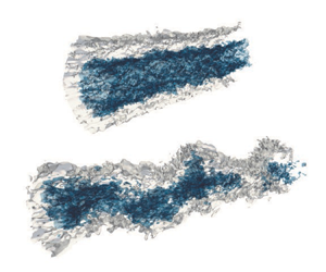
Regarding (iii), the emergence or decay of coherent structures is a major structural change. The three-dimensional visualisation of figure 9 shows the emergence of a helical structure coinciding with the $U_d\sim x^{-2/3}$ to $U_d\sim x^{-6/5}$ transition. The near wake (figure 9(a), also evident in figure 3a,b) is quasi-parallel without any visible large-scale azimuthal asymmetry. This near-wake topology is similar to that found by Kumar & Mahesh (Reference Kumar and Mahesh2018) and Posa & Balaras (Reference Posa and Balaras2016). However, farther downstream (figure 9b) a sinuous single helix, originating at $x\approx 20$, is observed. Previous simulations and experiments did not access locations downstream of $x\approx 20$ and, hence, did not observe the emergence of helical structures in the intermediate wake region.

Figure 9.

Isocountours of instantaneous streamwise velocity: (a) the near wake, white $0.97U_\infty$, blue $0.7 U_\infty$; and (b) the intermediate wake, white $0.97U_\infty$, blue $0.85 U_\infty$.

To further characterise the sinuous mode, figure 10(a) shows the cross-sectional area-integrated energy of the streamwise velocity fluctuations as a function of the azimuthal mode ($m$). Initially, at $x=3.5$, the turbulence is nearly broadband. As the wake evolves, energy concentrates around the $|m|=1$ mode and, progressively, the single helical mode dominates. The spectra (figure 10b) of $u_x$ confirms this finding. After $x=10$, a peak at $St=fD/U=0.28$ is visible and is sustained until the end of the domain. $St = 0.28$ corresponds to the wavelength of the undulation identified in figure 9(b).

Figure 10.

(a) Cross-wake area-integrated energy of $u_x$ as a function of the azimuthal wavenumber $|m|$. (b) Energy spectra of $u_x$ at $r = 0.5$.

We can further investigate the structure of the wake by looking into the spatio-temporal evolution of the azimuthal modes. Figure 11(a,c,e,g) show the time evolution of the Fourier coefficients of the axisymmetric $m=0$ mode and the single helix $|m|=1$ mode. The $r-t$ variation of these modes is plotted at two streamwise locations: $x=3.5$ and $x=30$, representative of the near and the intermediate wake, respectively. The characteristic frequencies of these modes are also identified by performing a temporal Fourier transform. The corresponding spectra are shown in figure 11(b,d,f,h).

Figure 11.

Azimuthal Fourier coefficients of modes $|m|=0$ and $|m|=1$ as a function of the radial coordinate and time at a fixed streamwise location: (a,c) near wake at $x=3.5$, which is $0.5D$ downstream from the trailing end of the body; (e,g) intermediate wake at $x=30$. Corresponding power spectra of the modes computed at specific radial locations, marked by the dotted black line: (b,d) near-wake spectra computed at $r=0.1$; (f,h) intermediate-wake spectra at $r = 0.5$.

In the near wake at $x=3.5$, which is $0.5D$ from the trailing end of the spheroid, the $|m|=0$ axisymmetric mode is broadband and carries the small-scale turbulence of the boundary layer, see figure 11(a,b). The $|m|=1$ mode (figure 11c), however, has distinctive low-frequency motions in the wake core. This low frequency is caused by the oscillation of the recirculation region, which is small and spans $r \approx 0.1$ as was shown in figure 3(b). In the spectra of figure 11(d), two low-frequency peaks are observed: $St=0.16$ and $St=0.28$. At $x=3.5$, both $m=0$ and $|m|=1$ have energy levels comparable with the other nearby modes, as was shown in figure 10(a).

At $x=30$, the small scales of the boundary layer have been dissipated and the $|m|=1$ low-frequency motion spans the whole wake width. A peak with a characteristic frequency of $St=0.28$ is clearly identified in figure 11(h) and is visible in the periodic stripes of figure 11(g). This peak is also observed farther downstream, as was shown in figure 10(b) and corresponds to the undulation observed in the wake visualisations, figures 3(c) and 9(b). In this region, the asymmetric $|m|=1$ mode contributes the most to the energy of the flow. Note that the origin of the $St=0.28$ oscillation can be traced to the near wake. However, its effect as a coherent structure is not visible until $x \approx 20$.

It is well established by experiments and linear stability analysis (Sato & Okada Reference Sato and Okada1966; Wygnanski et al. Reference Wygnanski, Champagne and Marasli1986; Monkewitz Reference Monkewitz1988; Berger et al. Reference Berger, Scholz and Schumm1990; Rigas et al. Reference Rigas, Oxlade, Morgans and Morrison2014), that the wake of axisymmetric bodies is dominated by a global instability with azimuthal wave number $|m|=1$. In bluff-body wakes, the $|m|=1$ mode dominates the flow starting right at the recirculation region where there is strong asymmetric shedding of the boundary layer (Rigas et al. Reference Rigas, Oxlade, Morgans and Morrison2014; Nidhan et al. Reference Nidhan, Chongsiripinyo, Schmidt and Sarkar2020). In this wake, however, the recirculation region is much smaller, and the asymmetry induced by the separated flow is weaker. The asymmetry is particularly weak because the flow immediately behind the body is surrounded by an axisymmetric region of turbulence originating from the turbulent boundary layer. As a result, the large-scale symmetry breaking of the wake associated with the presence of a coherent helical structure, becomes dominant only farther downstream, at $x\approx 20$, when the imprint of the boundary-layer turbulence becomes sufficiently weak.

The dominance of the $|m|=1$ mode in the intermediate wake coincides with the change of the decay rate and precedes the non-equilibrium scaling of dissipation. The relation between the non-equilibrium scaling of dissipation and the presence of coherent structures was hypothesised by Goto & Vassilicos (Reference Goto and Vassilicos2016) in three-dimensional decaying turbulence and more recently by Cafiero & Vassilicos (Reference Cafiero and Vassilicos2019) in turbulent jets. Here also, there is evidence of such a connection. In previous bluff-body wake studies (Chongsiripinyo & Sarkar Reference Chongsiripinyo and Sarkar2020; Nidhan et al. Reference Nidhan, Chongsiripinyo, Schmidt and Sarkar2020), the dominance of the helical $|m|=1$ instability and the establishment of a region of non-equilibrium scaling occurs very early in the wake. In the slender-body wake, the helical mode develops farther downstream and so does the non-equilibrium region. Note the strong contribution to the energy of the $|m|=1$ mode at $x=30$ in figure 10(a) immediately before the non-equilibrium scaling becomes appropriate.

Farther downstream, near the end of the domain, as shown in figure 10(a), the dominance of $|m|=1$ recedes. Therefore, the far wake might eventually transition to the classic $U_d\sim x^{-2/3}$. Simulations or experiments with longer domains are needed to clarify this.