2. Numerical method and problem set-up

We perform 3D numerical simulations of deformable RBCs in a simple shear flow $\boldsymbol{u}=\{\dot{{\it\gamma}}y,0,0\}$ , where $\dot{{\it\gamma}}$ is the shear rate, using a front-tracking method as described previously by Yazdani & Bagchi (Reference Yazdani and Bagchi2013) and Cordasco et al. (Reference Cordasco, Yazdani and Bagchi2014). The cell is modelled as a viscous liquid drop enclosed by a zero-thickness elastic membrane having the experimentally observed biconcave discocyte shape as the resting shape. The viscosity of the membrane is neglected in this study (except when mentioned otherwise). The interior and suspending fluids are assumed to be incompressible and Newtonian with viscosities ${\it\lambda}{\it\mu}_{o}$ and ${\it\mu}_{o}$ , respectively. The membrane is assumed to possess a resistance against shear deformation, area dilatation and bending. The shear deformation and area dilatation are modelled following Skalak et al. (Reference Skalak, Tozeren, Zarda and Chien1973) using an in-plane strain energy function,

where $G_{s}$ is the membrane shear elastic modulus, $I_{1}={\it\epsilon}_{1}^{2}+{\it\epsilon}_{2}^{2}-2$ and $I_{2}={\it\epsilon}_{1}^{2}{\it\epsilon}_{2}^{2}-1$ are the strain invariants of the Green strain tensor, and ${\it\epsilon}_{1}$ and ${\it\epsilon}_{2}$ are the principal stretch ratios. The area dilatation parameter $C$ is chosen so that the total surface area change remains less than 1 %. We choose $C=1000$ for capillary number $\mathit{Ca}=1$ and scale $C$ linearly with $\mathit{Ca}$ . Specific results are provided in supplementary materials available at http://dx.doi.org/10.1017/jfm.2014.587 to show that the total surface area and cell volume changes are of the order of 0.1 % for the cells in the intermittent regime (figures S33, S34, S35). The bending resistance is modelled following Helfrich’s formulation for bending energy (Zhong-can & Helfrich Reference Zhong-can and Helfrich1989),

where $E_{b}$ is the bending modulus, ${\it\kappa}$ is the mean curvature, $c_{o}$ is the spontaneous curvature and $S$ is the surface area. Computation of the membrane forces from (2.1) and (2.2) is described in Yazdani & Bagchi (Reference Yazdani and Bagchi2013). The fluid motion interior and exterior to the cell is obtained by solving the full Navier–Stokes equations. The computational domain is a cubic box of length $2{\rm\pi}a_{o}$ , where $a_{o}$ is the radius of a sphere having the same volume as the cell. The domain is discretized by $120^{3}$ points, and the cell surface is discretized using 20 480 triangular elements. The dimensionless time is denoted by $t^{\ast }=t\dot{{\it\gamma}}$ . The major dimensionless parameters are the capillary number $\mathit{Ca}=\dot{{\it\gamma}}\,{\it\mu}_{o}\,a_{o}/G_{s}$ and the viscosity ratio ${\it\lambda}$ . The effect of inertia is negligible. The ranges of $\mathit{Ca}$ and ${\it\lambda}$ considered here are 0.02–1 and 0.01–5, respectively, corresponding to a shear rate of approximately $1{-}1000\ \text{s}^{-1}$ . The stress-free state of the cell is assumed to be an oblate spheroid of reduced volume $V_{0}=V_{obl}/(A^{3/2}/3\sqrt{4{\rm\pi}})=0.997$ , where $V_{obl}$ is the spheroid volume and $A=134.1\ {\rm\mu}\text{m}^{2}$ is the surface area of a normal RBC. The choice of a reduced volume of 0.997 derives from our earlier work by Cordasco et al. (Reference Cordasco, Yazdani and Bagchi2014) where we compared erythrocyte dynamics in shear flow under different stress-free states of reduced volumes 0.997, 0.98, 0.95 and 0.644 (corresponding to the experimentally observed discocyte shape), and showed that the buckling of the cell shape near the transition border disappears as the reduced volume approaches that of a sphere. We observed that the use of a perfect sphere as the stress-free state leads to numerical instability when the cell is released in a flow. The reduced volume of 0.997 is very close to that of a sphere which still gives a stable result under dynamic flow conditions. The biconcave resting shape is generated numerically from the spheroid by deflation until the desired volume $V_{cell}=94.1\ {\rm\mu}\text{m}^{3}$ of a normal RBC is reached. The final shape agrees well with the experimental shape and has a reduced volume of 0.644 as of a normal RBC. The reference shape for the Helfrich energy is set by the inclusion of the spontaneous curvature $c_{o}$ as in (2.2). It should be noted that the resting shape is obtained under a balance between the membrane forces, and thus the shape is determined by the dimensionless bending stiffness $E_{B}/a_{o}^{2}G_{s}$ and the dimensionless spontaneous curvature $c_{o}a_{o}$ . The bending stiffness used in the simulations is approximately $6\times 10^{-19}\ \text{J}$ which is within the experimental range of $3{-}8\times 10^{-19}\ \text{J}$ . 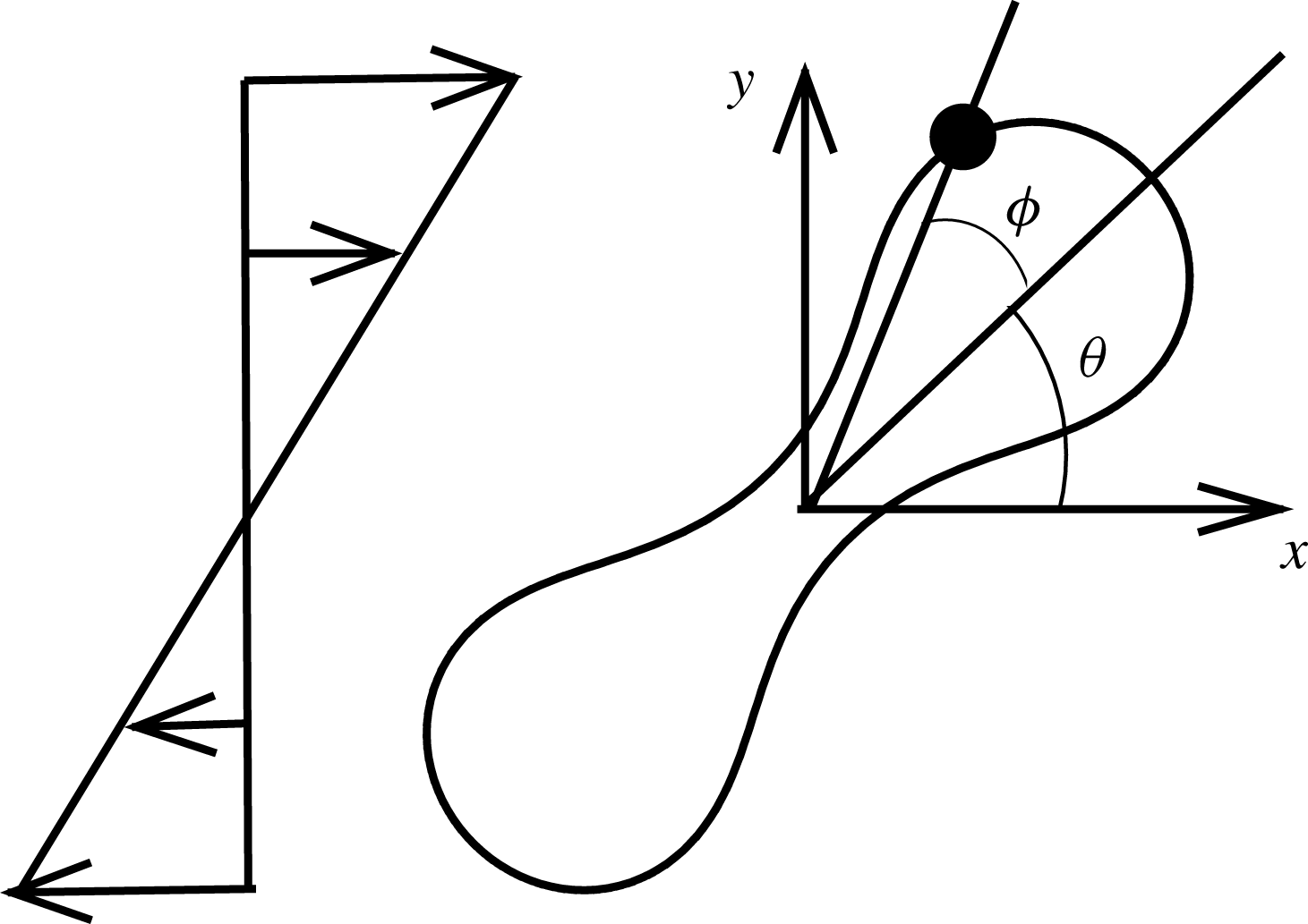The axis of revolution of the RBC initially lies in the shear plane. The cell dynamics is identified using two angles: the inclination angle ${\it\theta}$ of the RBC major axis with respect to the flow direction and the phase angle ${\it\phi}$ of a marker point on the cell surface with respect to the major axis (figure 1). For a swinging motion, ${\it\theta}$ oscillates but ${\it\phi}$ varies between $\pm {\rm\pi}/2$ , indicating a full rotation of the membrane. For a tumble, ${\it\phi}$ oscillates but ${\it\theta}$ varies between $\pm {\rm\pi}/2$ .

Figure 1.

Schematic of a biconcave RBC in shear flow, and definitions of ${\it\theta}$ and ${\it\phi}$ . Here, ⚫ represents a marker point on the cell surface.

3. Results and discussion

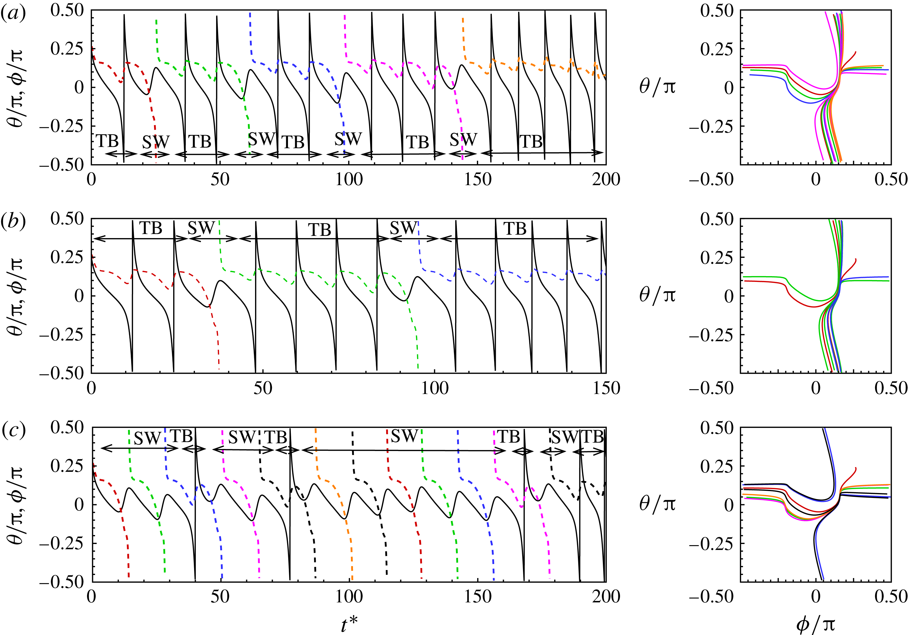
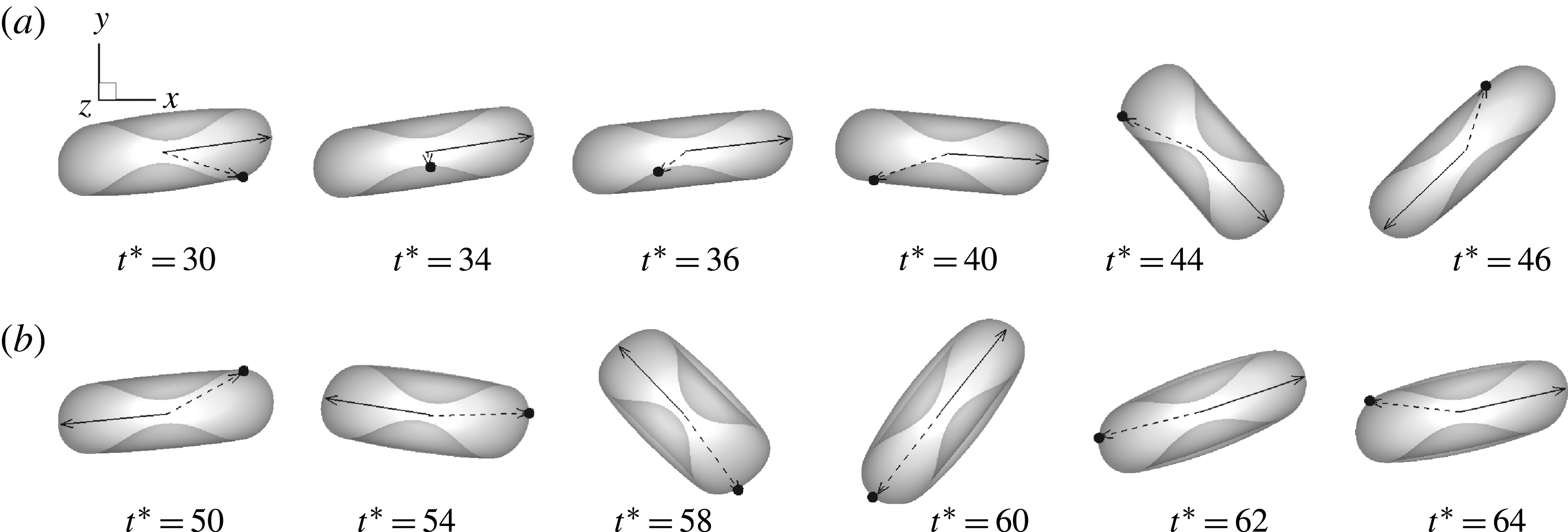
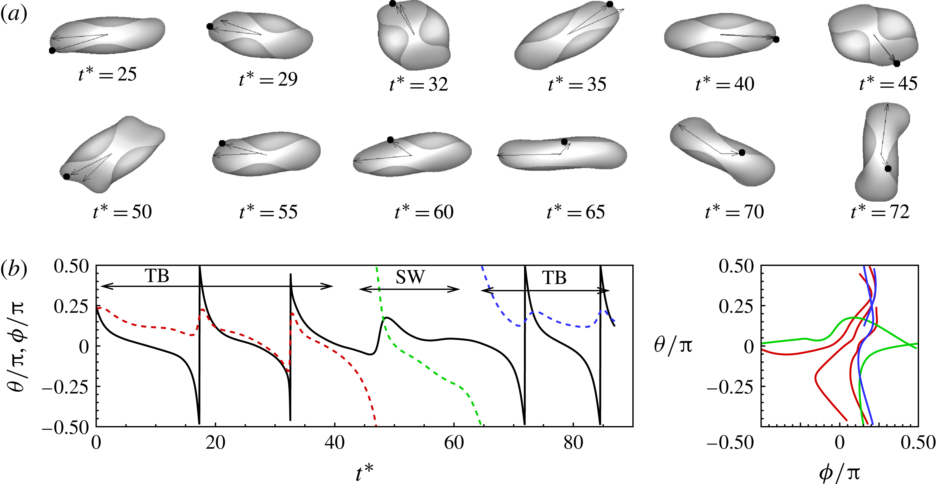
We observe intermittent and synchronized motions of the RBC in our simulations near the TB–TT border. In the current work, the intermittent motion is characterized by an irregular sequence of TB interrupted by an SW, or vice versa. The synchronized motion is periodic and is characterized by the coexistence of cell rotation and membrane rotation with an integer ratio of the rotational frequencies. Intermittent dynamics is shown in figure 2 for three representative cases. Additional cases are presented in the supplementary materials (figures S4–S16, and two animations). In figure 2(a), the cell swings once after one, two or three 180° tumbles. In figure 2(b), a sequence of TB is interrupted by a swing. In figure 2(c), a sequence of SW is interrupted by TB. Comparison of figures 2(b) and (c) shows the effect of changing $\mathit{Ca}$ : at lower $\mathit{Ca}$ , the cell mostly exhibits TB interrupted by SW; at higher $\mathit{Ca}$ , the cell mostly exhibits SW interrupted by TB. Further, during the SW phases, the cell sometimes swings about ${\it\theta}=0$ , while at other times it swings with ${\it\theta}>0$ . 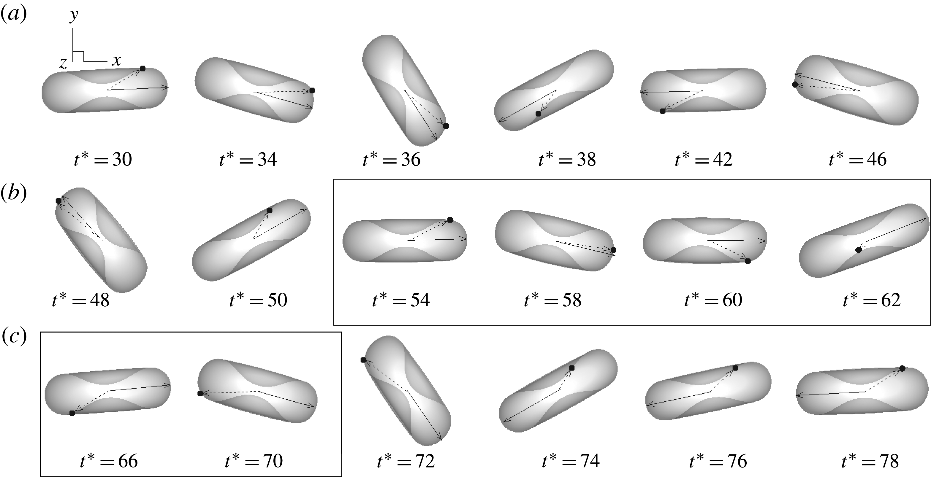A sequence of visualization is presented in figure 3 for the case in figure 2(a). The cell tumbles clockwise (CW) between $t^{\ast }\approx 30$ and 58, swings counter-clockwise (CCW) between $t^{\ast }\approx 58$ and 62, and resumes CW tumble for $t^{\ast }\gtrsim 70$ . The oscillation in ${\it\phi}$ during TB is evident from the back-and-forth movement of a marker point shown on the cell surface. In the SW phase, the marker point moves CW in a continuous manner resembling the membrane tank-tread and traverses nearly half of the cell contour (between $t^{\ast }\approx 54$ and 70). As TB resumes, the one-way rotation of the marker ends and the oscillatory motion resumes.

Figure 2.

Intermittent motion. The left panel shows the time evolution of the inclination angle ${\it\theta}$ (solid black line) and phase angle ${\it\phi}$ (coloured dashed lines). The right panel shows the trajectory in a ${\it\theta}{-}{\it\phi}$ phase plot. (a) $\mathit{Ca}=0.029$ , ${\it\lambda}=0.42$ . (b)  $\mathit{Ca}=0.0302$ , ${\it\lambda}=0.6$ . (c) $\mathit{Ca}=0.0325$ , ${\it\lambda}=0.6$ . A visualization sequence for case (a) is shown in figure 3, and for case (c) in figure S16 in the supplementary materials.

Figure 3.

Intermittent motion at $\mathit{Ca}=0.029$ , ${\it\lambda}=0.42$ . The full simulation is shown in figure 2(a) until $t^{\ast }\approx 200$ . The cell tumbles CW between $t^{\ast }\approx 30$ and 58, swings CCW between $t^{\ast }\approx 58$ and 62, and resumes CW tumble for $t^{\ast }\gtrsim 70$ . The swinging phase is marked by a box. The cell axis is marked by a solid line and a marker point on the cell surface is tracked. See the supplementary materials for an animation.

Prior full-scale numerical study by Kessler et al. (Reference Kessler, Finken and Seifert2008) found that initially tumbling capsules eventually settled into a stable swinging motion. The analytical model by Vlahovska et al. (Reference Vlahovska, Young, Danker and Misbah2011) which allows for small deformation of capsules also concluded that intermittency is a transient event and capsules settled into stable SW after a few initial tumbles. In contrast, the present results show that the cells switch between TB and SW in a truly intermittent manner. Figure 2 shows that our simulations can predict a sequence of tumbles interrupted by swinging, as well as a sequence of swings interrupted by tumbling. Furthermore, we find that the exact behaviour of the cell is highly sensitive to the parameters: for example, in figures 2(b) and (c), as $\mathit{Ca}$ changes from 0.0302 to 0.0325, the dynamics changes from a TB sequence interrupted by SW to an SW sequence interrupted by TB.

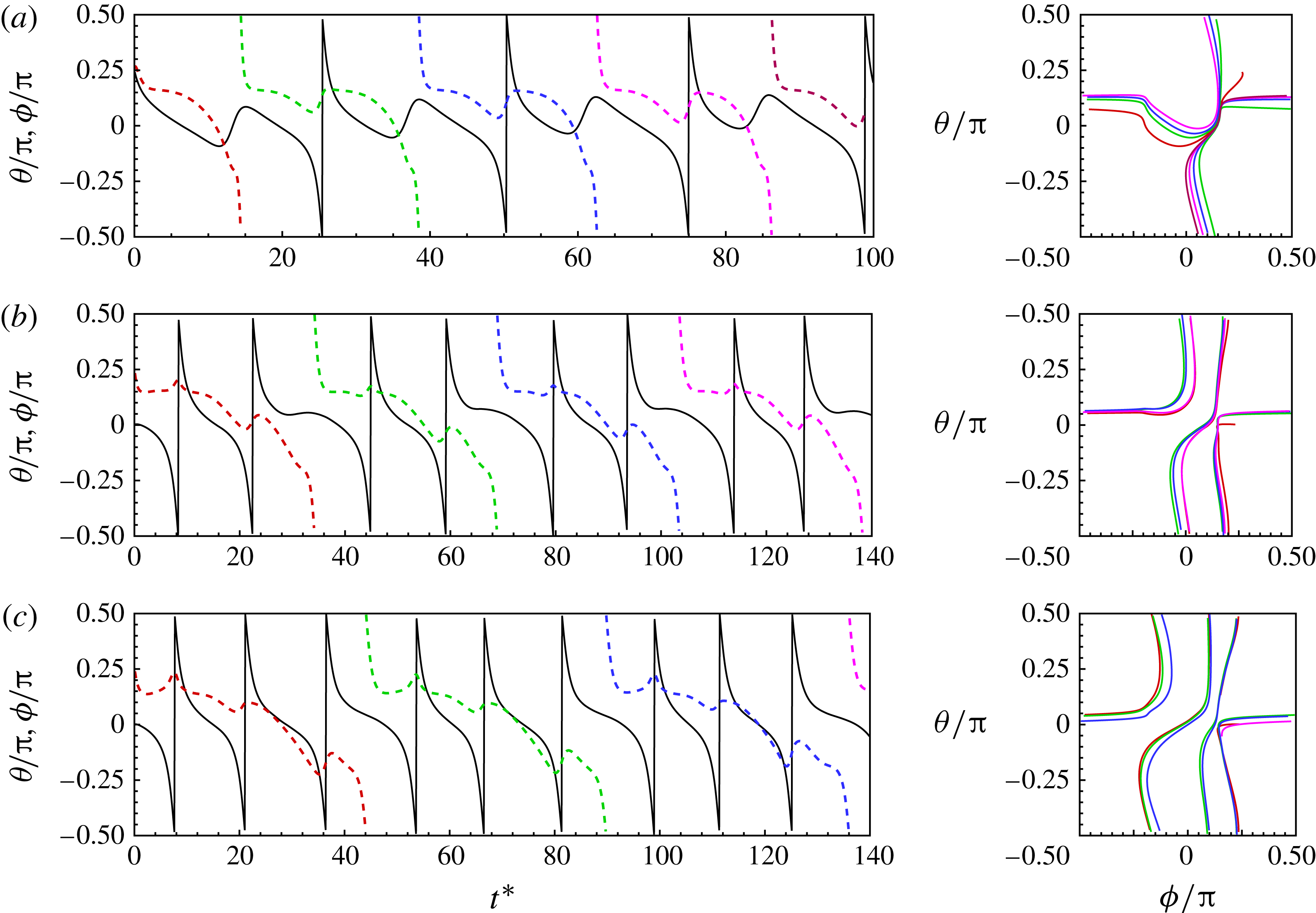
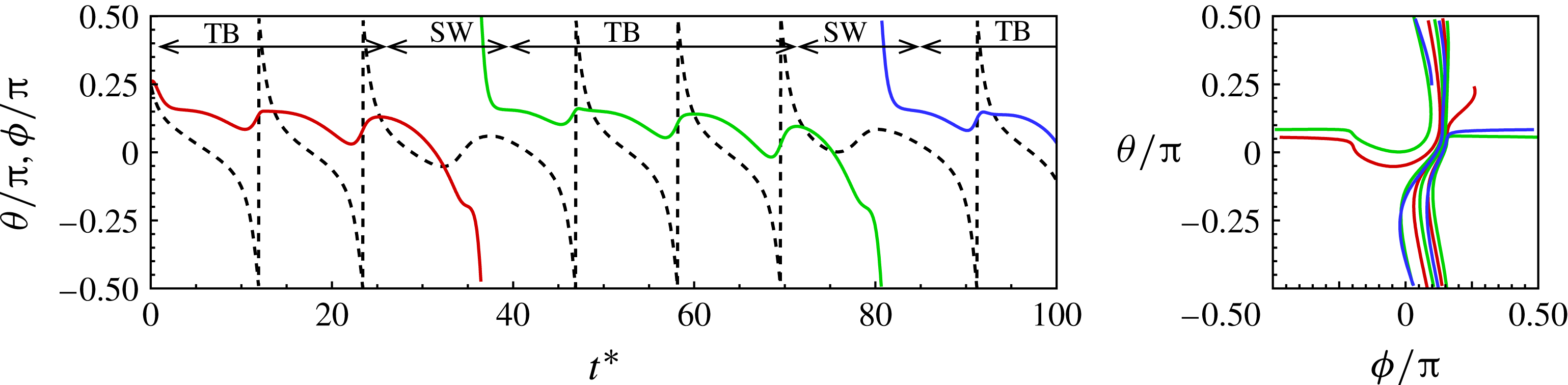
A synchronized motion characterized by one 180° tumble followed by one swing is shown in figure 4(a). During the SW phase, the cell swings CCW while the membrane makes the one-way CW rotation resembling a TT and traversing nearly half of the cell contour. In the TB phase, the cell rotates CW as the axis crosses $\pm {\rm\pi}/2$ , while the membrane rotates CCW by a small angle. The net rotation of the membrane over a complete cycle is CW. Thus membrane rotation and cell tumbling exist simultaneously. For the specific case shown in figure 4(a), the tumbling frequency is equal to the membrane rotational frequency, i.e. $f_{{\it\theta}}/f_{{\it\phi}}=1$ . Additional cases of synchronized motion and coexistence of TT and tumbling are presented in figures 4(b) and (c) in which the membrane rotation progressively slows down, resulting in increasing values of $f_{{\it\theta}}/f_{{\it\phi}}=2$ and 3, respectively. Similarly to the prediction made by Noguchi (Reference Noguchi2009, Reference Noguchi2010), integer values of $f_{{\it\theta}}/f_{{\it\phi}}$ are observed, which in the present simulations vary from 1 to 6. These additional cases of synchronized motion are presented in the supplementary materials (figures S17–S32 and two animations). Here, two or more tumbles are followed by a ‘slower’ tumble during which the cell spends a longer time along the flow direction and the membrane rotates by a significant amount. A sequence of visualization for $f_{{\it\theta}}/f_{{\it\phi}}=2$ (for the case in figure 4 b) is shown in figure 5 (see the supplementary materials for an animation). As is evident, the cell major axis crosses ${\it\theta}=\pm {\rm\pi}/2$ twice (indicating a full 360° rotation) as the membrane rotates by 180°.

Figure 4.

Synchronized motion resulting in integer ratios of the tumbling frequency and membrane rotation frequency. (a) Periodic TB and SW which results in $f_{{\it\theta}}/f_{{\it\phi}}=1$ . Panels (b) and (c) illustrate coexistence of TB and TT where $f_{{\it\theta}}/f_{{\it\phi}}=2$ and 3, respectively. (a) $\mathit{Ca}=0.03$ , ${\it\lambda}=0.5$ ; (b) $\mathit{Ca}=0.073$ , ${\it\lambda}=1.73$ ; (c) $\mathit{Ca}=0.087$ , ${\it\lambda}=2.38$ . The line patterns are as explained in figure 2.

Figure 5.

Synchronized motion with coexistence of TB and TT at $\mathit{Ca}=0.063$ , ${\it\lambda}=1.73$ . The full simulation is shown in figure 4(b). The membrane rotates 180° as the cell axis makes a full 360° rotation resulting in $f_{{\it\theta}}/f_{{\it\phi}}=2$ . An animation is given in the supplementary materials.

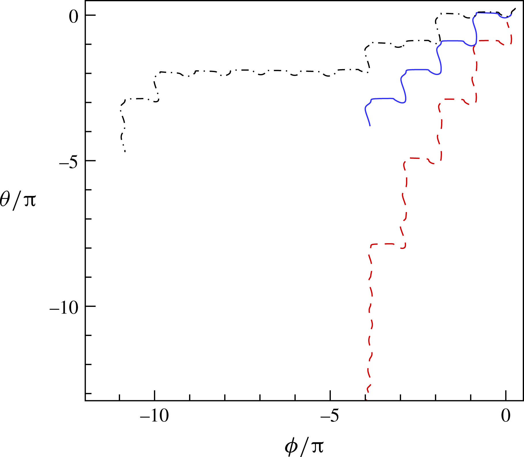
To further differentiate between the intermittent and synchronized motions, we provide an extended ${\it\theta}{-}{\it\phi}$ plot in figure 6. The trajectory for the synchronized motion (corresponding to the case shown in figure 4 a) shows identical steps representing a periodic behaviour. The trajectories for the intermittent motion (corresponding to the cases shown in figures 2 a,c) show unequal steps.

Figure 6.

Extended phase plot in continuous ${\it\theta}$ and ${\it\phi}$ comparing the synchronized motion (solid line, corresponding to the case shown in figure 4 a) and intermittent motion (dashed and dash–dotted lines, corresponding to the cases shown in figures 2 a,c, respectively).

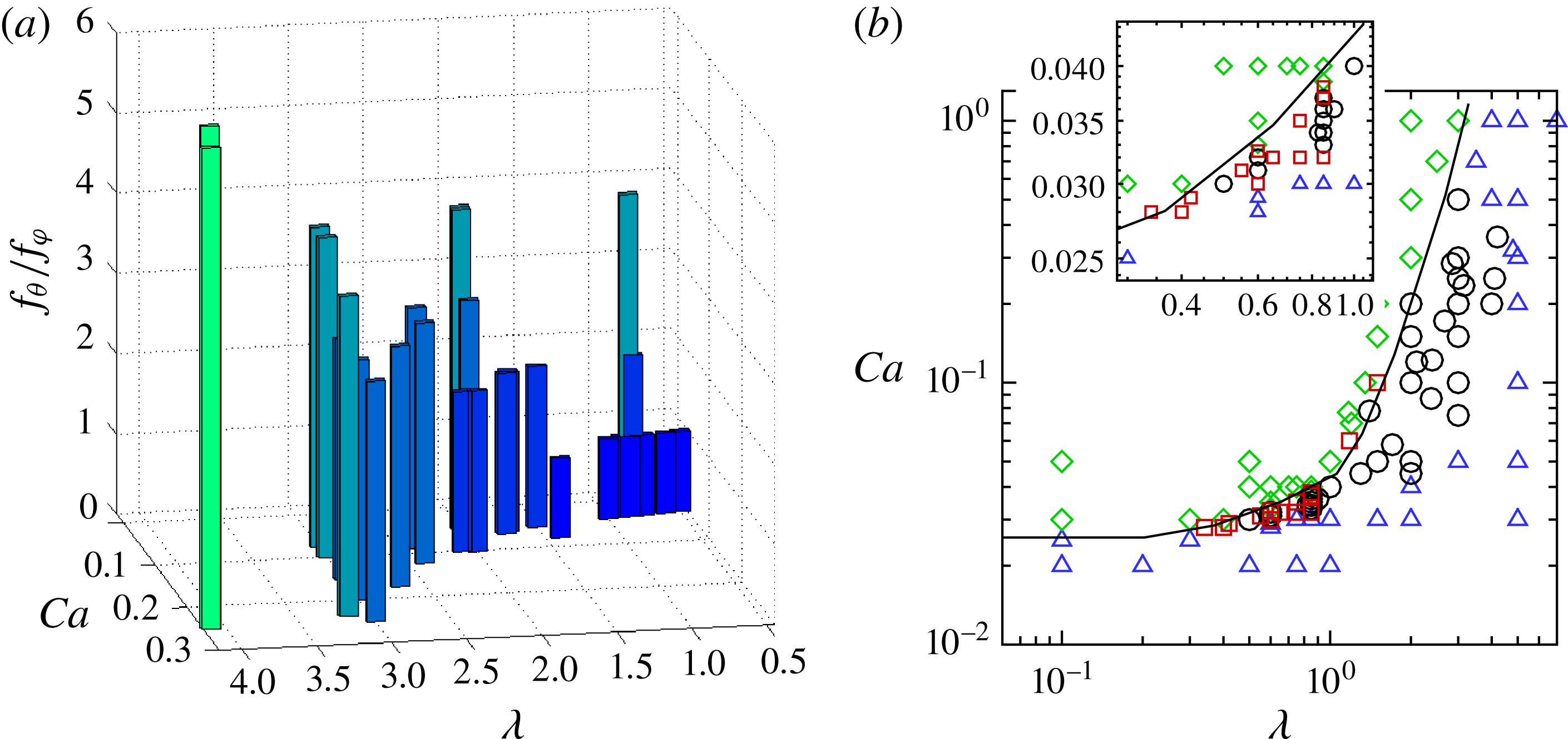
Figure 7(a) shows $f_{{\it\theta}}/f_{{\it\phi}}$ obtained from our simulations as a function of $\mathit{Ca}$ and  ${\it\lambda}$ . The frequency ratio varies from 1 to 6 in the parameter range considered in the simulations, resembling a Devil’s staircase as predicted by the reduced model of Noguchi (Reference Noguchi2009, Reference Noguchi2010). The figure shows that $f_{{\it\theta}}/f_{{\it\phi}}$ increases with increasing ${\it\lambda}$ , but decreases with increasing $\mathit{Ca}$ . Consequently, pure TB ( $f_{{\it\theta}}/f_{{\it\phi}}\longrightarrow \infty$ ) is approached as ${\it\lambda}$ increases or $\mathit{Ca}$ decreases, and pure TT ( $f_{{\it\theta}}/f_{{\it\phi}}\longrightarrow 0$ ) is approached as ${\it\lambda}$ decreases or $\mathit{Ca}$ increases. The figure shows that the synchronized motion is also very sensitive to the parameters, as small changes in $\mathit{Ca}$ and ${\it\lambda}$ can greatly alter $f_{{\it\theta}}/f_{{\it\phi}}$ .

Figure 7.

(a) Ratio of cell tumbling frequency to membrane rotation frequency, $f_{{\it\theta}}/f_{{\it\phi}}$ , in synchronized motion as a function of $\mathit{Ca}$ and ${\it\lambda}$ . (b) Phase diagram in the $\mathit{Ca}{-}{\it\lambda}$ plane illustrating different dynamics: pure SW (green diamonds), pure TB (blue triangles), intermittent dynamics (red squares), synchronized dynamics (black circles). The solid line is drawn manually as an approximate TT–TB transition border. The inset shows a zoomed-in section where the intermittent dynamics is observed.

Figure 7(b) shows a phase diagram in the $\mathit{Ca}{-}{\it\lambda}$ plane illustrating the parameter range for the intermittent and synchronized motions. Dynamics obtained from nearly 100 simulations are presented here. Intermittency is observed near the TT–TB transition border in a narrow range of $\mathit{Ca}$ , and for ${\it\lambda}\lesssim 1$ . A variety of rich dynamics consisting of synchronized tumbling with TT and intermittent tumbling and swinging can exist. There is a progression from tumbling with increasing membrane oscillation to tumbling with intermittent swinging with increasing $\mathit{Ca}$ . Tumbling accompanied by TT then appears in which the cell tends toward synchronized rotations with integer ratios of rotational frequency. Eventually, the RBC exhibits swinging with intermittent tumbles which transitions to pure swinging with a further increase in $\mathit{Ca}$ . The sensitivity of the dynamics to $\mathit{Ca}$ and ${\it\lambda}$ is evident from the inset of figure 7(b), where a small part of the phase diagram is enlarged.

Figure 8.

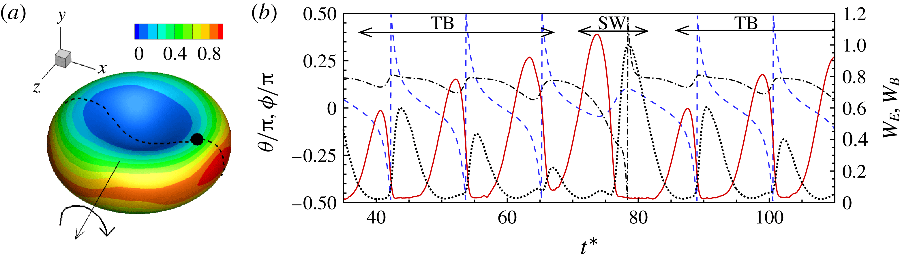
(a) Distribution of membrane elastic energy $W_{E}$ as given by (2.1). The trajectory of a membrane patch is indicated. (b) The time evolution of the elastic energy $W_{E}$ (red solid line, right axis) and bending energy $W_{B}$ (black dotted line, right axis) of a membrane patch, cell inclination angle ${\it\theta}$ (blue dashed line, left axis) and phase angle of the patch (black dash–dotted line, left axis) are shown for a synchronized motion of $f_{{\it\theta}}/f_{{\it\phi}}=3$ . ${\it\lambda}=0.85,\mathit{Ca}=0.033$ .

It should be noted that the range of shear rate over which intermittent and synchronized dynamics are observed is below the physiological range, but consistent with the in vitro study of Abkarian et al. (Reference Abkarian, Faivre and Viallat2007). However, low shear rates can occur in venules, and under pathological conditions. The synchronized motion is observed to persist closer to the physiological range, although the membrane rotation becomes much slower ( $f_{{\it\theta}}/f_{{\it\phi}}=6$ at ${\it\lambda}\approx 4$ in the figure). It should be noted that the phase diagram presented here is for the cell with a nearly spherical stress-free state (reduced volume 0.997). For a comparison of the phase diagrams for the nearly spherical stress-free state and the discocyte stress-free state, we refer to our earlier work by Cordasco et al. (Reference Cordasco, Yazdani and Bagchi2014), where we showed that the TB–TT transition occurs at lower $\mathit{Ca}$ for the former case than the latter. There, we also presented a comparison of our phase diagram with experimental data by Abkarian et al. (Reference Abkarian, Faivre and Viallat2007), Dupire et al. (Reference Dupire, Socol and Viallat2012) and Fischer & Korzeniewski (Reference Fischer and Korzeniewski2013). Peng et al. (Reference Peng, Mashayekh and Zhu2014) as well as Tsubota et al. (Reference Tsubota, Wada and Liu2013) also found that the TB–TT border shifts to lower $\mathit{Ca}$ for the nearly spherical stress-free state. Here, we do not repeat these results, as the purpose of figure 7(b) is to show the parametric range where the intermittency occurs, and not to compare the phase boundaries obtained from different studies.

Figure 9.

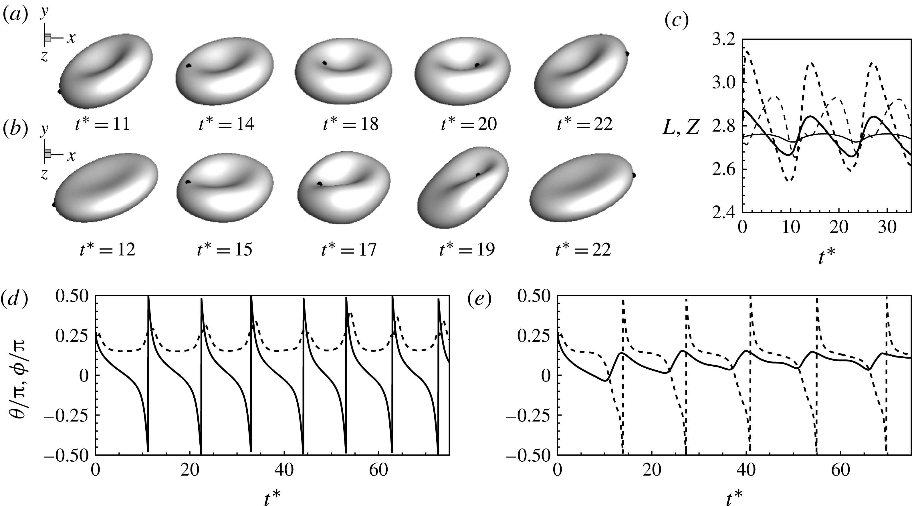
(a)–(c) Comparison of the RBC dynamics near the transition border for the SSF state (a, $\mathit{Ca}=0.03$ , ${\it\lambda}=0.1$ ) and for the BCSF state (b, $\mathit{Ca}=0.15$ , ${\it\lambda}=0.1$ ). As noted earlier, the transition border shifts to lower $\mathit{Ca}$ for the SSF state. The maximum elongations ( $L$ , thick lines) in the shear plane and along the vorticity direction ( $Z$ , thin lines) are compared in (c) for the SSF state (continuous lines, $\mathit{Ca}=0.04$ , ${\it\lambda}=0.75$ ) and BCSF state (dashed lines, $\mathit{Ca}=0.15$ , ${\it\lambda}=0.75$ ). (d), (e) Sample results showing the non-existence of intermittency for the BCSF state. TB is observed in (d) ${\it\lambda}=0.6$ and $\mathit{Ca}=0.11$ ; SW is observed in (e) ${\it\lambda}=0.6$ and $\mathit{Ca}=0.12$ .

We now provide a physical explanation of the observed dynamics. Figure 8(a) shows the membrane (in-plane) elastic energy $W_{E}$ as given by (2.1), which is relatively small in and around the dimple, but increases rapidly and substantially near the rim, resembling an energy well (see also figure S3 in the supplementary materials). In a pure TT case, the hydrodynamic shear force is high enough so that the membrane elements are able to overcome the energy barrier. Conversely, in a pure TB case, the hydrodynamic shear force is weaker, and the membrane elements can only oscillate and show zero net movement. Figure 8(b) shows the time evolution of the local elastic energy of a membrane patch for a synchronized dynamics of $f_{{\it\theta}}/f_{{\it\phi}}=3$ . Unlike in pure TB, here a net forward displacement occurs after each back-and-forth oscillation and the membrane element climbs slightly higher up the energy barrier with each tumble. After three tumbles, the element finally moves over the rim, and then it slides rapidly downhill into the energy well of the other dimple. The slide downhill causes the cell to tank-tread without a tumble. Once within the energy well, the membrane element again oscillates in an attempt to climb the energy hill while the cell executes another TB sequence. Interestingly, as is evident from figure 8(b), the elastic energy achieves a local maximum preceding each vertical flip of the RBC until it eventually exceeds the barrier indicated by a global maximum at which point the cell swings. Also shown in figure 8(b) is the time evolution of the bending energy of the membrane patch $(2{\it\kappa}-c_{o})^{2}\text{d}S$ . The bending energy has the opposite trend to the elastic energy: it is maximum near the dimple and minimum around the rim. However, bending energy alone does not provide a barrier to membrane rotation, as noted by Noguchi (Reference Noguchi2010) and also illustrated in our previous study by Yazdani & Bagchi (Reference Yazdani and Bagchi2011), where we observed that the TB–TT transition border at low ${\it\lambda}$ remained nearly unchanged with increasing bending stiffness.

We find that the intermittent and synchronized dynamics occur when the stress-free state of the cell is close to a sphere (hereafter called the SSF state), but not the biconcave discocyte (hereafter called the BCSF state). Our simulations and those of Peng et al. (Reference Peng, Mashayekh and Zhu2014) show that near the TB–TT transition, the RBC undergoes a large shape deformation and significant departure from the resting biconcave shape under the BCSF state. In contrast, the shape oscillation is significantly reduced and an almost stable biconcave shape is maintained under the SSF state (figure 9). In particular, the breathing motion is reduced for the SSF state, as is evident from the snapshots, as well as from the time-dependent cell lengths. For the BCSF case, the cell exhibits a greater inward folding (at around $t^{\ast }\approx 17$ in the figure), and the cell lengths show wider fluctuations indicating breathing-like dynamics. Earlier, in Cordasco et al. (Reference Cordasco, Yazdani and Bagchi2014), we explained the reduced deformation for the SSF state based on the membrane energy. In and around the dimple, the bending energy is very high for the SSF state. Furthermore, the rim of the cell is under a large tensile stress for the former, but under a compressive stress for the latter. The presence of the compressive stress cause the large shape oscillation and breathing dynamics under the BCSF state, while the higher bending energy and tensile stress suppress them for the SSF state. Indeed, the very recent experimental work by Dupire et al. (Reference Dupire, Socol and Viallat2012) shows that RBCs maintain their stable biconcave shape near the transition, and concludes that the biconcave discocyte is not the stress-free state. While the exact stress-free shape still remains controversial (see, e.g., Fischer & Korzeniewski Reference Fischer and Korzeniewski2013), our results show that the intermittent and synchronized motion can occur only under certain stress-free states. As mentioned earlier, the specific value of the reduced volume considered here is 0.997, which is very close to that of a sphere. This specific value is not important, and the results presented here would remain unchanged as long as the stress-free state considered remains close to a sphere. As the reduced volume is decreased, the region of intermittency also decreases. In the limit where the stress-free state approaches the discocyte, the intermittency is absent. Also shown in figures 9(d) and (e) is the angle plot for the BCSF state near the transition border as this is the region where intermittency is expected. As is evident, for two close values of $\mathit{Ca}$ (0.11 and 0.12), we get pure TB and SW, respectively; no intermittency is observed. If a value of $\mathit{Ca}$ is chosen to match the intermittent region for the SSF state, a pure TB dynamics is observed, since the transition border is shifted to higher $\mathit{Ca}$ for the BCSF state, as discussed before. More detailed results comparing the dynamics of the two stress-free states are given in Cordasco et al. (Reference Cordasco, Yazdani and Bagchi2014), and can also be found in Peng et al. (Reference Peng, Mashayekh and Zhu2014), and, hence, are not repeated here.

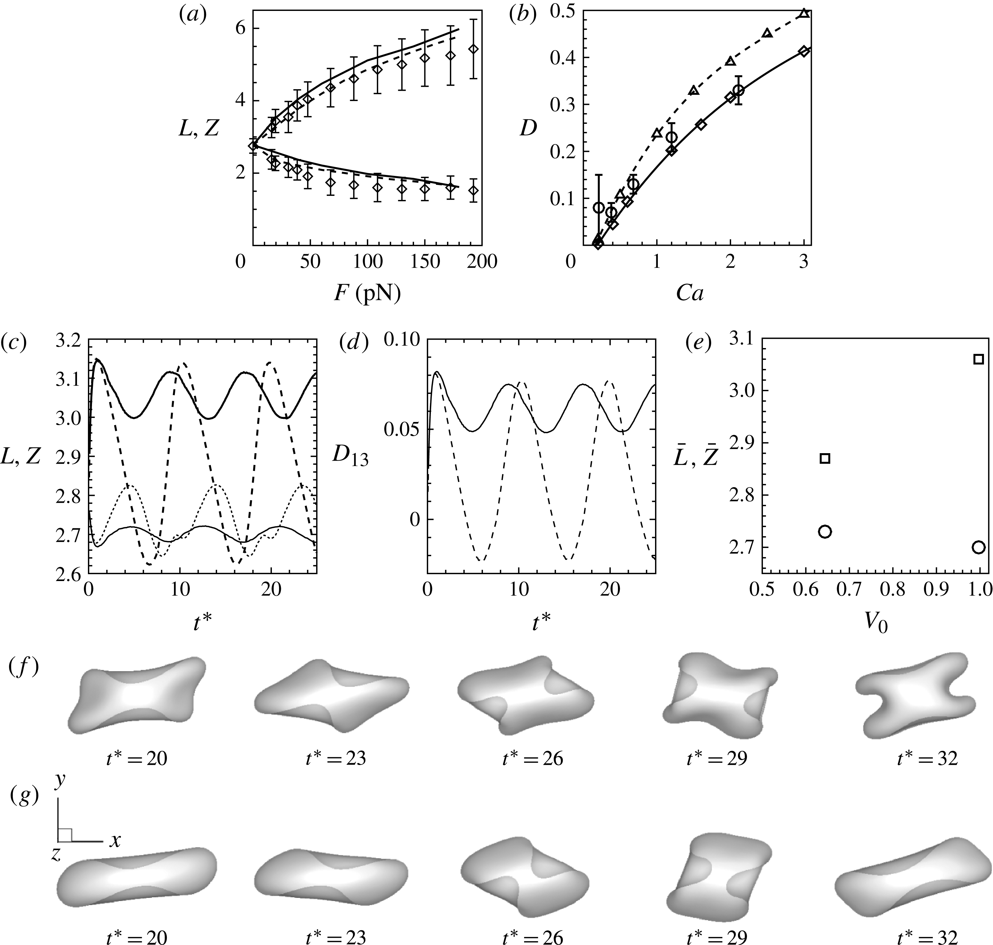
It should be emphasized that the SSF state does not limit cell deformation, in general. It only eliminates the breathing-like dynamics that occurs for the BCSF state near the transition border. The SSF state does not yield an ‘almost shape-preserved cell’ as used in the reduced-order analysis. To illustrate this point we provide a number of results in figure 10. First, we simulate cell stretching experiments using optical tweezers, and present the cell length under the SSF and BCSF states comparing our numerical data with the experimental data of Mills et al. (Reference Mills, Qie, Dao, Lim and Suresh2004) in figure 10(a). The data show that the deformation of the cell using the spherical stress-free state is very close to that obtained using the discocyte stress-free state. Second, figure 10(b) compares the cell elongation in shear flow under the two stress-free states, and also compares the results with the experimental data of Wang et al. (Reference Wang, Zhao, Zhuang and Stoltz1999) at high shear rates. Here, the spherical stress-free state yields slightly higher elongation than the discocyte state. Then, in figures 10(c) and (d), we plot the time-dependent elongation of the cell in the shear plane and along the vorticity axis, and the deformation parameter for both the SSF and BCSF states at moderate shear rates. The corresponding time-averaged elongations are given in figure 10(e), which again shows that the spherical stress-free state yields higher average elongation than the discocyte state.

Figure 10.

(a) Simulation of optical tweezer stretching experiments of RBC using the spherical stress-free state (dashed lines) and discocyte state (solid lines). The numerical data are compared with the experimental data of Mills et al. (Reference Mills, Qie, Dao, Lim and Suresh2004) (symbols with error bars). The cell elongation predicted by the SSF state is close to that predicted by the BCSF state. (b) Time-averaged cell deformation in shear flow at high shear rates using the spherical stress-free state (- -▵- -) and the discocyte stress-free state (—♢—). Numerical data are compared with laser diffraction measurements of Wang et al. (Reference Wang, Zhao, Zhuang and Stoltz1999) (○ with error bars). The SSF state predicts higher elongation than the BCSF state. (c)–(e) Comparison of the red blood cell dynamics away from the transition border at a moderate shear rate for the SSF and BCSF states. $\mathit{Ca}=0.2$ , ${\it\lambda}=0.1$ . (c) The time-dependent cell elongation in the shear plane ( $L$ , thick lines) and along the vorticity direction ( $Z$ , thin lines) for the SSF (continuous lines) and BCSF (dashed lines) states. (d) The time-dependent deformation parameter $D_{13}=(L-Z)/(L+Z)$ . (e) The time-averaged $L$ (▫) and $Z$ (○) for the SSF ( $V_{0}=0.997$ ) and BCSF ( $V_{0}=0.644$ ) states. The SSF state predicts higher average elongation than the BCSF state. (f,g) The time-dependent cell shapes for the SSF and BCSF states, respectively, at ${\it\lambda}=5$ , $\mathit{Ca}=1.0$ . Cell deformation is more severe for the SSF state.

Finally, in figures 10(f) and (g), we show cell shapes at moderately high shear rates and physiological viscosity ratio. Here, the SSF state shows more severe deformation than the BCSF state. Thus, the spherical stress-free state used here is not merely an ‘almost shape-preserved’ model like what is usually used in theoretical studies.

Figure 11.

Effect of higher bending stiffness on the dynamics of cells with the BCSF state. (a) Time evolution of the cell shape and (b) inclination and phase angles. Here, $E_{B}/a_{o}^{2}G_{s}=0.05$ , ${\it\lambda}=4.5,Ca=0.5$ . The line patterns are the same as in figure 2.

It should also be noted that several prior studies including the ones by Dupire et al. (Reference Dupire, Socol and Viallat2012), Tsubota et al. (Reference Tsubota, Wada and Liu2013), Cordasco et al. (Reference Cordasco, Yazdani and Bagchi2014) and Peng et al. (Reference Peng, Mashayekh and Zhu2014) indicated that the stress-free state of the RBC is close to that of a sphere. Thus, the spherical stress-free state considered here is not a mere postulation. However, the present study is the only one to show that such a state leads to intermittency.

Moreover, cell deformation is introduced in the reduced models in an empirical manner. Further, the reduced-order models do not account for the stress-free state explicitly. The present study is the first to show that the intermittency is directly connected to the stress-free state through an exact model of a fully deformable cell, in stark contrast to the reduced-order models.

We now comment on the role of the bending stiffness. Noguchi (Reference Noguchi2010) related the disappearance of the intermittent dynamics to low values of the bending modulus used by Kessler et al. (Reference Kessler, Finken and Seifert2008). The dimensionless bending stiffness used in their simulation is 0.01, whereas that used in ours is 0.03. Hence, these two values are not significantly different. Thus, the bending stiffness alone cannot account for the observed intermittency in the present work. We have performed additional simulations using the BCSF state by varying the dimensionless bending stiffness from 0.002 to 0.05. See also Yazdani & Bagchi (Reference Yazdani and Bagchi2011) for a detailed study on the effect of the bending stiffness. It appears that for the BCSF state, cells near the TB–TT transition border undergo extreme buckling at low to moderate values of bending stiffness. Buckling persists even with higher values of the bending stiffness, as shown in figure 11. Although the inclination and phase angles seem to suggest a TB sequence interrupted by an SW, we cannot strongly say that intermittency occurs here due to buckling. This observation is consistent with the discussion in Fischer & Korzeniewski (Reference Fischer and Korzeniewski2013) in reference to the work by Fedosov et al. (Reference Fedosov, Caswell and Karniadakis2010). In contrast, we clearly see intermittency for the cells with the SSF state with a value of the bending stiffness that is within the experimental range and also close to those used by others in their simulations. It should be noted that for the SSF state, the resting biconcave shape can be generated only under certain choices of the dimensionless bending stiffness, the reduced volume and the spontaneous curvature (see, e.g., Seifert, Berndl & Lipowsky Reference Seifert, Berndl and Lipowsky1991). For a smaller value of the bending stiffness, the discocyte shape can be generated by using also a smaller value of the reduced volume, and the corresponding cell shows buckling when subjected to a shear flow. On the other hand, the simulations become unstable if a much higher value ( $E_{B}/a_{o}^{2}G_{s}>0.05$ ) of the bending stiffness is used.

We now discuss the role of membrane viscosity. The results presented so far were obtained without considering the membrane viscosity. It should be noted that the definition of ${\it\lambda}$ used here is simply the ratio of the internal (haemoglobin) to external (suspending) fluid viscosities, ${\it\lambda}={\it\mu}_{i}/{\it\mu}_{o}$ . The membrane viscosity does not enter in the definition of ${\it\lambda}$ . In simulations where the membrane viscosity is considered, we introduce an additional dimensionless parameter ${\it\mu}_{m}^{\ast }={\it\mu}_{m}/{\it\mu}_{o}a_{o}$ , where ${\it\mu}_{m}$ is the dimensional membrane viscosity. Thus, in our scaling, we have two parameters, ${\it\lambda}$ and ${\it\mu}_{m}^{\ast }$ . Alternatively, one can introduce a single parameter, an effective viscosity, which in dimensionless form can be written as an effective viscosity ratio as ${\it\lambda}_{eff}={\it\lambda}+{\it\Phi}_{memb}/{\it\Phi}_{internal}$ , where ${\it\Phi}$ is the viscous dissipation. Both approaches are correct, and the specific choice depends on the implementation of the different constituents of the membrane model. Experiments on shear flow dynamics of the RBC usually report the viscosity value of the suspending fluid, from which ${\it\lambda}$ can be directly obtained as per our definition without knowing the membrane viscosity. Abkarian et al. (Reference Abkarian, Faivre and Viallat2007) provided experimental data on intermittency for a suspending medium viscosity of 22 mPa s and at a shear rate of ${\sim}1.5\ \text{s}^{-1}$ , which yields $\mathit{Ca}=0.03$ and ${\it\lambda}\approx 0.3$ as per our definition. Furthermore, the theoretical study by Skotheim & Secomb (Reference Skotheim and Secomb2007) noted intermittency in the range ${\it\lambda}\sim 1$ . Therefore, the range of ${\it\lambda}$ and $\mathit{Ca}$ in which intermittency is observed in the present simulations agrees with that in prior experimental and theoretical studies.

To address whether the membrane viscosity alters the observed intermittency, we have performed additional simulations including the membrane viscosity. The details of the numerical implementation of the membrane viscosity can be found in our previous study by Yazdani & Bagchi (Reference Yazdani and Bagchi2013). A sample result is presented in figure 12. It is evident that intermittency is present even when the membrane viscosity is considered in the simulations.

Figure 12.

Sample result showing that intermittency could be present when the membrane viscosity is considered. Here, $\mathit{Ca}=0.04$ , ${\it\lambda}=0.5$ , and ${\it\mu}_{m}^{\ast }=10$ . The line patterns are the same as in figure 2.

Finally, it should be noted that in experiments by Dupire et al. (Reference Dupire, Socol and Viallat2012), it was shown that the stable orientation of the cell at low $\mathit{Ca}$ is the rolling orientation, and the transition occurs as SW to rolling. In our previous studies by Cordasco & Bagchi (Reference Cordasco and Bagchi2013) and Cordasco et al. (Reference Cordasco, Yazdani and Bagchi2014) we studied this SW to rolling transition in great detail for RBCs (under different stress-free configurations), and for prolate and oblate spheroids, and explained this behaviour based on energy considerations. In those studies, we found that the shear plane orientation is a metastable orientation, and that a small deviation from this metastable configuration could lead to cell movement towards the rolling orientation. However, if the background noise is low and grows very slowly over time, the in-shear-plane TB dynamics can be sustained in this metastable configuration. Furthermore, by a detailed parametric search performed in Cordasco & Bagchi (Reference Cordasco and Bagchi2013) and Cordasco et al. (Reference Cordasco, Yazdani and Bagchi2014) we did find that the TB dynamics could be stable for ${\it\lambda}\lesssim 1$ and small values of $\mathit{Ca}$ (see the phase diagrams given in these papers).

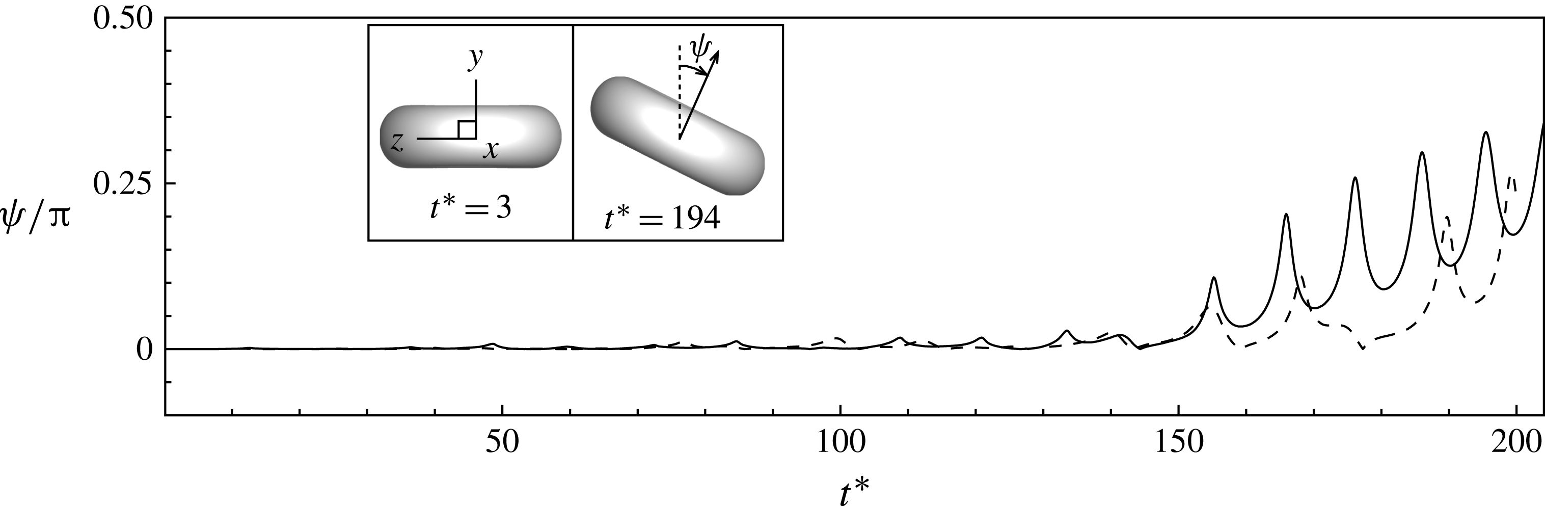
Nonetheless, if the current simulations are extended over a longer time, we do observe cell movement towards the rolling orientation near the end of the simulation, as shown in figure 13. The results shown here correspond to the intermittent cases presented in figures 2(a) and (c). The growth of the off-shear-plane angle ${\it\psi}$ as shown in the figure suggests the remarks made above about the role of inherent noise in the system. A rapid increase in the off-shear-plane angle occurs near the end of the simulation at which point the cell starts a precessing motion about the vorticity axis. If the simulations are continued even further, the cells settle in the rolling orientation as shown in Cordasco & Bagchi (Reference Cordasco and Bagchi2013) and Cordasco et al. (Reference Cordasco, Yazdani and Bagchi2014). It should be noted that for a long time the cell axis remains aligned with the shear plane allowing us a sufficiently large time window to clearly observe intermittency for several cycles. For additional results and physical insights on the transition from SW to rolling orientation, we refer the reader to Cordasco & Bagchi (Reference Cordasco and Bagchi2013) and Cordasco et al. (Reference Cordasco, Yazdani and Bagchi2014).

Figure 13.

Cell movement from the shear plane towards the rolling orientation. Shown here is the angle ${\it\psi}$ that the cell axis of revolution makes with the shear plane, ${\it\psi}=0$ when the axis is aligned in the shear plane and ${\rm\pi}/2$ when it is aligned with the vorticity axis. The results are shown for the intermittent cases presented in figures 2(a) (solid line) and (c) (dashed line). The insets show the cell shape/orientation looking along the flow direction ( $x$ ) near the beginning and end of the simulation, and illustrate tilting of the cell axis away from the shear plane and towards the vorticity axis ( $z$ ). Intermittent dynamics occurs over a large time window before the cell moves significantly off plane and starts a precessing dynamics. See Cordasco & Bagchi (Reference Cordasco and Bagchi2013) and Cordasco et al. (Reference Cordasco, Yazdani and Bagchi2014) for details.