



1. Introduction
Axial solute dispersion in micro/nano-fluidic systems holds significant theoretical importance and practical applications, with its regulation directly influencing the efficiency of critical processes such as micro-mixing (Dong et al. Reference Dong, Zhang, Wang and Luo2014; Liao et al. Reference Liao, Dasgupta, Srinivasan and Liu2015), separation analysis (Ghosal & Chen Reference Ghosal and Chen2012; Dhellemmes et al. Reference Dhellemmes, Leclercq, Lichtenauer, Hochsmann, Leitner, Ebner, Michel Martin, Neusu and Cottet2024) and electrophoresis (Ghosal Reference Ghosal2006). Over recent decades, alongside the rapid advancement of microfluidic technology, this field has demonstrated broad application prospects in scenarios such as biomedicine, chemical synthesis and point-of-care diagnostics. Meanwhile, active control strategies for axial dispersion have continuously evolved, including: modulating flow characteristics via applied pressure gradients (Rana & Murthy Reference Rana and Murthy2016a ; Azari & Sadeghi Reference Azari and Sadeghi2022); regulating solute diffusion behaviour using electric fields (Rubinstein & Zaltzman Reference Rubinstein and Zaltzman2013); introducing magnetic fields to induce Lorentz forces and alter solute diffusions (Vargas et al. Reference Vargas, Arcos, Bautista and Méndez2017); engineering interfacial interactions through surface modification techniques (Sadeghi et al. Reference Sadeghi, Saidi, Moosavi and Sadeghi2020).
In microfluidic systems, electro-osmosis (EO) attracts significant research interest due to its unique capability for pump-free fluid propulsion. Introducing magnetic fields to establish an additional magnetohydrodynamic (MHD) effect creates a novel fluid manipulation mechanism, enabling fine-scale regulation of hydrodynamic characteristics through the interaction between electromagnetic fields and fluids. Additionally, the synergistic combination of hydrophobic wall slip characteristics and slip-dependent zeta potential further enhances fluid behaviour control. Therefore, this study investigates how interface slip and slip-dependent zeta potential modulate solute dispersion in viscoelastic solutions under oscillatory electro-osmotic flow (EOF) coupled with MHD, developing enhanced technology for precise control of microscale mass transport.
1.1. Theoretical models for solute dispersion
Theoretical research on dispersion models has long attracted the attention of researchers. Taylor’s pioneering work (Taylor Reference Taylor1953) laid the foundation for solute dispersion modelling in pressure-driven pipe flows. This model relies on transverse concentration averaging, which requires an initial phase for radial diffusion to homogenise cross-sectional concentration profiles. This process is characterised by the dimensionless time scale
 $D_m t / R^2$
(where
 $t$
,
 $D_m$
and
 $R$
denote time, molecular diffusivity and pipe radius, respectively), restricting the model’s validity to long-time regimes. To overcome these limitations, Aris extended Taylor’s dispersion theory using the moment method for an infinitely long pipe (Aris Reference Aris1956). He derived a second-moment equation to describe the average concentration distribution under steady advection and demonstrated that, over sufficiently long times, solute tracers evolve into a Gaussian distribution due to the mean flow field. This research further refined the applicability and descriptive capability of Taylor dispersion theory. Subsequently, the methodologies based on the models proposed by Taylor and Aris were improved by Chatwin (Reference Chatwin1970), Barton (Reference Barton1983), Jimenez & Sullivan (Reference Jimenez and Sullivan1984), Mazumder & Das (Reference Mazumder and Das1992) and Wu & Chen (Reference Wu and Chen2014).
Over the years, numerous studies have examined solute transport behaviour under different conditions, such as porous layers (Dentz et al. Reference Dentz, Icardi and Hidalgo2018; Das et al. Reference Das, Mondal, Poddar and Wang2024a ), MHD flows (Vargas et al. Reference Vargas, Arcos, Bautista and Méndez2017; Poddar et al. Reference Poddar, Saha, Mondal, Dhar and Mazumder2024; Das et al. Reference Das, Poddar and Kairi2024b ; Sen et al. Reference Sen, Mondal and Kairi2025), pollutant emissions in floating wetlands (Ai et al. Reference Ai, Dai, Zhai, Chen and Huai2022), by improving Taylor’s model. However, these studies have only analysed solute diffusion at long times after injection into the fluid and have not provided any information on solute diffusion during the short time immediately following injection. Notably, Samuel et al. (Reference Samuel, Chang, Ma and Santiago2025) recently extended the Taylor dispersion in coupled electro-osmotic and pressure-driven flows across all time regimes under the assumptions of a low zeta potential, the Debye-Hückel approximation and a finite electric double layer (EDL) thickness. Initial studies sought to characterise band broadening dynamics immediately following injection, Gill & Sankarasubramanian (Reference Gill and Sankarasubramanian1970) put forth a general model, which articulates the transport coefficients as functions of time within steady-state flow. Subsequently, a series of advancements have been made. These include the consideration of a time-variable flow (Gill & Sankarasubramanian Reference Gill and Sankarasubramanian1972; Sankarasubramanian & Gill Reference Sankarasubramanian and Gill1972; Vedel & Bruus Reference Vedel and Bruus2012), oscillating flow (Rana & Murthy Reference Rana and Murthy2016a ; Azari & Sadeghi Reference Azari and Sadeghi2022), the non-uniformity of the injected solute band (Gill & Sankarasubramanian Reference Gill and Sankarasubramanian1971, Reference Gill and Sankarasubramanian1972) and interfacial/boundary mass transfer processes (Sankarasubramanian & Gill Reference Sankarasubramanian and Gill1973; Rana & Murthy Reference Rana and Murthy2016a ). In the present study, we are set to carry out a comprehensive exploration of the solute dispersion driven by the combined effects of MHD and oscillating EOF. Our research builds upon the generalised dispersion model that was introduced by Gill & Sankarasubramanian (Reference Gill and Sankarasubramanian1970).
1.2. Solute dispersion in microchannels driven by EOF and MHD
The manipulation of fluid flow and dispersion in microchannels via EOF represents a foundational area of inquiry in microfluidics owing to its attributes of operational simplicity, high controllability, uniform flow velocity profiles and reliance on non-mechanical actuation (Sadr et al. Reference Sadr, Yoda, Zheng and Conlisk2004; Goyal et al. Reference Goyal, Datta and Chakraborty2024; Mehta & Mondal Reference Mehta and Mondal2024). For nearly a century, the literature has systematically investigated various aspects of hydrodynamic dispersion in direct-current (DC) EO. Huang et al. (Reference Huang, Debnath, Roy, Wang, Jiang, Beg and Kuharat2024) showed that in transient Taylor–Gill dispersion during EOF, the peak concentration attenuates with increasing reaction intensity. Through multiscale analysis, Subudhi et al. (Reference Subudhi, Jangili and Barik2024) found that stronger coupling parameters significantly slow solute transport in micropolar EOF within rectangular microchannels. Ponalagusamy & Murugan (Reference Ponalagusamy and Murugan2023) revealed that the EDL effect enhances solute diffusion in Carreau fluid under combined pressure-driven flow and EOF. Schulz et al. (Reference Schulz, Gärttner and Ray2024) developed a novel effective dispersion model accounting for Taylor–Aris dispersion, EO-induced dispersion and their coupling. They theoretically proved the positivity of the dispersion coefficient and the existence and uniqueness of strong solutions, and numerically demonstrated the feasibility of charged species separation. Additionally, researchers have persistently pursued inquiries in this domain to examine the impacts of diverse supplementary facets of electrokinetic phenomena on solute transport and mixing dynamics (Arcos et al. Reference Arcos, Méndez, Bautista and Bautista2018; Mukherjee et al. Reference Mukherjee, DasGupta and Chakraborty2020; Mozafari et al. Reference Mozafari, Safarzadeh and Sadeghi2025).
Beyond conventional DC-EOF systems, alternating-current (AC)-EOF governs dynamic dispersion through electric field and EDL interactions to optimise dispersion and mixing processes in microfluidic systems. Li & Jian (Reference Li and Jian2017) presented a focused investigation into solute dispersion induced by AC-EOF of viscoelastic fluids, with series expansion and transform techniques employed for analysis. Reshadi & Saidi (Reference Reshadi and Saidi2019) found that in oscillatory EO-Poiseuille flow through polyelectrolyte-grafted capillaries, the polyelectrolyte layer (PEL) enhances solute advection and dispersion. A thicker charged PEL strengthens electro-osmotic advection, flattening transverse concentration and increasing radial differences. Mederos et al. (Reference Mederos, Arcos, Bautista and Méndez2020) theoretically investigated mass transfer in a microcapillary connecting two reservoirs with different concentrations of an electro-neutral solute. Results show that fluid elasticity–oscillatory flow interplay can enhance mass transfer rates by orders of magnitude compared with Newtonian oscillatory EOF. Peralta et al. (Reference Peralta, Arcos, Méndez and Bautista2020) investigated the mass transfer of Maxwell fluids in concentric annular microchannels driven by an AC-EOF. The analysis demonstrates that optimising the elasticity number, cylindrical gap and angular Reynolds number rationally can augment the total mass transfer rate and facilitate component separation. Subsequently, extensive research on solute transport driven by AC-EOF has primarily focused on the following key directions: dispersion analysis in microchannels with diverse geometries (Vargas et al. Reference Vargas, Méndez, Docoslis and Escobedo2023), solute dispersion in nanochannels enclosed by a dielectric liquid layer (Chowdhury et al. Reference Chowdhury, Pal and Gopmandal2025), the coupling effects of non-uniform walls (Dehe et al. Reference Dehe, Rehm and Hardt2021), regulatory mechanisms of asymmetric wall zeta potentials and slip interfaces (Huang et al. Reference Huang, Kuo and Huang2022), as well as the regulatory mechanisms of high zeta potentials and slip interfaces (Saha & Kundu Reference Saha and Kundu2022) on solute transport properties. In this work, an AC electric field is employed due to its superior performance in solute dispersion and microfluidic control. Its periodic polarity reversal suppresses electrode polarisation and electrolysis, thereby avoiding the unstable EOF and band broadening associated with DC fields. The oscillating field drives solutes into reciprocating motion, enhancing mixing and dispersion efficiency. Electrokinetic effects can be flexibly tuned by adjusting the frequency and amplitude, while high-frequency operation reduces Joule heating and improves system stability. These merits make AC electric fields highly suitable for microfluidic and biological applications.
In recent years, electric fields, magnetic fields and their synergy are widely used to precisely control microfluidic flows, with broad prospects in chemical and biomedical engineering involving mass and heat transport. In the study of EO and MHD flows, Joule heating and viscous dissipation constitute key thermal and mechanical effects. Chakraborty et al. (Reference Chakraborty, Dey and Chakraborty2013) reported that under constant wall heat flux, both effects reduce the Nusselt number via distinct mechanisms: Joule heating uniformly elevates bulk fluid temperature and weakens the wall temperature gradient, while viscous dissipation intensifies near the wall and raises wall temperature, both deteriorating heat transfer. Xie & Jian (Reference Xie and Jian2017) quantified entropy generation in two-layer MHD and EOF with Joule heating, finding that the entropy generation rate decays from the wall to interface and is dominated by the Hartmann number and viscous dissipation. Yang et al. (Reference Yang, Jian, Xie and Li2019) investigated MHD-EOF and heat transfer in rectangular microchannels, demonstrating that heat transfer is jointly affected by Joule heating, viscous dissipation and electromagnetic coupling, where increased viscous dissipation impairs heat transfer while a larger electrokinetic width promotes it. Rilwan et al. (Reference Rilwan, Oni, Jha and Jibril2024) further examined the influences of Joule heating and viscous dissipation on electromagnetohydrodynamic flow and heat transfer in porous microchannels. Furthermore, the coupled driving of MHD and EOF enables precise regulation of solute dispersion paths, thereby offering a new paradigm for the multi-field synergistic control of microscale mass transfer processes. Poddar et al. (Reference Poddar, Saha, Mondal, Dhar and Mazumder2024) showed that strong magnetic fields significantly reduce flow velocity and the Taylor dispersion coefficient in two-dimensional MHD Taylor dispersion through parallel channels. Vargas et al. (Reference Vargas, Arcos, Bautista and Méndez2017) and Das et al. (Reference Das, Poddar and Kairi2024b ) applied Aris’ method of moments to Newtonian solute dispersion in EO-MHD flows through parallel plate microchannels. Specifically, Vargas et al. (Reference Vargas, Arcos, Bautista and Méndez2017) found that slow sinusoidal wall zeta potential variations, combined with EO-MHD forces, significantly alter the axial distribution of the effective dispersion coefficient. Das et al. (Reference Das, Poddar and Kairi2024b ) explored the regulatory effects of symmetric and asymmetric zeta potentials on solute distribution, demonstrating that asymmetric zeta potentials accelerate the dispersion process. Subsequently, Sen et al. (Reference Sen, Mondal and Kairi2025) introduced heterogeneous first-order boundary reactions and transverse electric fields to further investigate the solute dispersion characteristics of non-Newtonian fluids under the combined effects of MHD and EOF in parallel plate microchannels. All their core conclusions are fundamentally based on Aris’ method. Notably, Joule heating has been consistently neglected in existing studies on solute dispersion in MHD and EOF-driven flows. This indicates that while Joule heating is indispensable in heat transfer-focused analyses of MHD and EOF systems, neglecting it in studies concentrating on solute dispersion is a common and reasonable practice. This simplification is not an oversight, but rather reflects the physical consensus in the field that thermal effects are always secondary to the hydrodynamic mechanisms of interest in such problems. In line with this established research paradigm, the present study focuses on elucidating the fundamental regulatory mechanism of electromagnetic forces on solute dispersion over a wide range of magnetic field intensities. Within the parameter range explored, the temperature rise induced by Joule heating is negligible, and it is therefore justifiably excluded from the analysis.
1.3. Microchannel interfacial slip and slip-dependent zeta potential
In microscale fluid mechanics, the extremely small characteristic scales (at the micrometre level) and high surface-area-to-volume ratios make surface properties a core determinant of flow behaviour. Notably distinct from macroscopic flows, hydrodynamic slip at microscale liquid–solid interfaces is a prevalent phenomenon, whereby traditional no-slip models often require modification due to their inadequacy (Thompson & Troian Reference Thompson and Troian1997; Zhu & Granick Reference Zhu and Granick2001, Reference Zhu and Granick2002). This attribute is critical in microscale EOF. First, interfacial slip directly alters the flow field. In hydrophobic microchannels, non-wetting conditions exacerbate the breakdown of the no-slip assumption, making slip length an essential parameter (Hegde & Harikrishnan Reference Hegde and Harikrishnan2021; Sujith et al. Reference Sujith, Mehta and Pati2025). Second, wall slip modifies the relationship between surface potential and zeta potential. Specifically, slip leads to an apparent increase in zeta potential, which manifests as a reduced velocity gradient within the EDL (Joly et al. Reference Joly, Ybert, Trizac and Bocquet2006).
The interplay between interfacial slip and zeta potential has been a focal point of research in recent decades. Owing to the strong coupling between these two factors, the independent measurement of electrokinetic phenomena on hydrophobic surfaces remains challenging. Early investigations by Churaev et al. (Reference Churaev, Ralston, Sergeeva and Sobolev2002) established a linear relationship model between slip length and zeta potential through experiments on methylated quartz capillaries. Subsequent studies by Yang & Kwok (Reference Yang and Kwok2002) and Tandon & Kirby (Reference Tandon and Kirby2008) further refined this theoretical framework. This mechanistic understanding highlights that traditional surface potential models based on the no-slip assumption are no longer capable of accurately describing microscale transport characteristics, with the interaction between interfacial slip and electrochemical properties emerging as a critical factor in explaining physical processes within microfluidic devices.
Recently, research on surface slip and slip-dependent zeta potential has made significant progress in the field of microscale fluid dynamics, spanning fluid flow, heat transfer mechanisms, energy conversion systems and solute dispersion processes in EOF, MHD flow and EO-MHD coupled flow. Banerjee et al. (Reference Banerjee, Mehta, Pati and Biswas2021) showed that traditional surface potential models (neglecting slip) underestimate core flow velocity in combined electro-osmotic pressure-driven microchannels. Banerjee et al. (Reference Banerjee, Pati and Biswas2023) found that slip-induced zeta potential increase strengthens EO force and enhances near-wall velocity in pulsatile EO and shear-driven flows. Siva et al. (Reference Siva, Dubey and Jangili2024) confirmed that slip-dependent zeta potential governs rotational flow and volume transport in EO-MHD couple stress flows in rotating microchannels. Deng et al. (Reference Deng, Xiao and Liang2024) demonstrated that slip-dependent zeta potential significantly enhances the sensitivity of two-layer flow parameters in unsteady cylindrical EOF. Other recent studies on the EO and MHD transport of viscoelastic fluids in microchannels with slip-dependent zeta potential have revealed several critical advances. The slip-dependent zeta potential significantly optimises the electrokinetic energy conversion process (Saha & Kundu Reference Saha and Kundu2023; Liu et al. Reference Liu, Wu and Liu2024; Saha & Kundu Reference Saha and Kundu2025); strengthening the coupling between interfacial charges and fluid slip remarkably modifies the electromagnetic transport properties (Das et al. Reference Das, Vajravelu and Kairi2025) and thermal entropy characteristics (Siva et al. Reference Siva, Jangili and Kumbhakar2023) in a microchannel.
Notably, the influence of interfacial slip on solute dispersion has sparked extensive discussion (Li & Jian Reference Li and Jian2019; Huang et al. Reference Huang, Kuo and Huang2022; Saha & Kundu Reference Saha and Kundu2022). The investigation of coupled slip-dependent zeta potential and viscoelastic effects of Carreau fluids in two-fluid EOF demonstrated that slip modifies diffusion kinetics by enhancing the apparent zeta potential, with shear-thinning/thickening behaviour further amplifying this effect (Kuntal et al. Reference Kuntal, Ghiya and Tiwari2025). However, the solute dispersion characteristics in the combined driving regime of AC-EOF and MHD with slip-dependent zeta potential remain unexplored in existing literature.
1.4. The position and structure of the current work
Based on a comprehensive review of recent advancements in solute dispersion studies within microfluidic systems, it has been found that EOF and the hybrid EO-MHD approach for fluid flow and mass transport have emerged as a prominent frontier in multi-physics microscale transport research. This synergistic strategy integrates the high driving efficiency of EO with the superior dispersion-suppression capability of MHD, enabling better controllability than single actuation modes. It exhibits great potential for applications including biochemical separation, targeted drug delivery and microfluidic reaction systems (Sahore et al. Reference Sahore, Doonan and Bailey2018; Chaudhuri et al. Reference Chaudhuri, Mandal and Bandyopadhyay2018; Zhang et al. Reference Zhang2025), where stable transport and tuneable dispersion are essential. Nevertheless, current research still suffers from several limitations, as detailed below.
First, a key challenge in this field is that, whereas research has predominantly focused on Newtonian fluids (Reshadi & Saidi Reference Reshadi and Saidi2019; Sadeghi et al. Reference Sadeghi, Saidi, Moosavi and Sadeghi2020; Das et al. Reference Das, Poddar and Kairi2024b ; Samuel et al. Reference Samuel, Chang, Ma and Santiago2025) and select non-Newtonian fluids (Sen et al. Reference Sen, Mondal and Kairi2025) within microchannels, the governing mechanisms of coupled magneto-electrodynamic fields on solute dispersion in viscoelastic fluids remain elusive. Given the prevalence of such fluids in industrial applications of axial dispersion, elucidating their behaviour is critical. This lack of mechanistic insight across broad parameter spaces hinders the development of general principles for dispersion.
Second, current research on the influence of microscale interfacial characteristics on solute dispersion processes remains insufficient. Most existing studies are based on the no-slip assumption (Reshadi & Saidi Reference Reshadi and Saidi2019; Sadeghi et al. Reference Sadeghi, Saidi, Moosavi and Sadeghi2020; Das et al. Reference Das, Poddar and Kairi2024b ; Samuel et al. Reference Samuel, Chang, Ma and Santiago2025; Sen et al. Reference Sen, Mondal and Kairi2025), which exhibits significant limitations in microscale flows. Moreover, the majority of related work has focused only on the role of single factors, such as heterogeneous or asymmetric zeta potentials at the wall (Vargas et al. Reference Vargas, Arcos, Bautista and Méndez2017; Das et al. Reference Das, Poddar and Kairi2024b ), without incorporating the combined effects of interfacial slip and zeta potentials.
Third, although Gill’s generalised dispersion model shows higher reliability in describing the transient processes of solute dispersion, its inherent complexity in mathematical derivation has resulted in limited adoption in practical microfluidic systems.
Against this backdrop, building on an extension of Gill’s generalised dispersion model, this study seeks to (i) systematically investigate the solute dispersion behaviour in polymer solutions within microchannels under the drive of MHD-AC-EOF multiphysics coupling, and (ii) further elucidate the regulatory role of microscale interfacial effects, specifically interfacial slip characteristics and slip-dependent zeta potential, in this dispersion process. The findings will offer more comprehensive theoretical underpinnings for optimising the separation and mixing performance of microfluidic devices.
The remainder of this paper is structured as follows. The subsequent section first systematically describes the flow geometry configuration and explicitly outlines the physical problem formulation along with key assumptions. Section 3 outlines the governing equations for MHD-AC-EOF and solute dispersion in polymer solutions; specifically, the development of models for several types of complex polymer solutions and the estimation of their corresponding parameters are detailed in Appendix A; additionally, the corresponding analytical solution algorithms are proposed. Section 4 presents the core results of this study, including the validation of the proposed model and corresponding simulation results, alongside an in-depth mechanism analysis underlying the effects of major dimensionless parameters on solute dispersion behaviour under both AC-EOF and mixed MHD-AC-EOF regimes. Finally, § 5 concludes the paper with discussions on the results.
The diagram of the MHD-AC-EOF in a microtube with a slip-dependent zeta potential.

Figure 1. Long description
A diagram of the MHD-AC-EOF in a microtube with a slip-dependent zeta potential. The microtube has an anode on the left and a cathode on the right. An alternating current electric field is applied along the length of the tube. The tube has a hydrophobic wall with a slip length δ. Positive and negative ions are distributed within the tube, with arrows indicating the direction of the magnetic field. The green shaded area represents the injected solute band. The diagram includes labels for the anode, cathode, AC field, hydrophobic wall, and magnetic field.
2. Problem description and assumptions
As shown in figure 1, the unsteady flow characteristics and dispersion phenomena in viscoelastic solutions (such as polymer solutions) through a microtube under the coordinated driving of an AC electric field and a magnetic field are considered. A cylindrical coordinate system is adopted, with its origin precisely situated at the centre of the tube. In this coordinate system,
 $r$
represents the radial distance measured from the central axis of the tube, while
 $x$
denotes the axial coordinate. The microtube has a radius
 $R$
and is sufficiently long such that the flow is fully developed and all physical quantities are independent of the axial coordinate
 $x$
. The dispersion process commences at
 $t=0$
with the instantaneous injection of a minute quantity of solute. This solute is uniformly distributed across the cross-section at
 $x=0$
and subsequently propelled by the MHD-AC-EOF within the flexible microtube. It is postulated that the injected solute band is sufficiently dilute such that the flow of the carrier fluid remains unaffected by the presence of trace-level soluble substances. In this study, the research objectives are pursued in a sequential manner. Initially, an analysis of the dynamic behaviours of MHD-AC-EOF is performed, which holds significant importance for studies on solute dispersion driven by MHD-AC-EOF. After that, the dispersion characteristics of the solutes injected into the tube will be analysed under two distinct scenarios: pure AC-EOF and mixed MHD-AC-EOF. The following sections elaborate on these aspects in detail.
3. Mathematical analysis of electric potential, velocity and concentration fields
Currently, we are preparing to conduct an analysis of MHD-AC-EOF and solute dispersion in a narrow tube with a slip-dependent zeta potential. The velocity for the MHD-AC-EOF and concentration for solute dispersion are determined by momentum conservation and mass transport. In the case of considering a symmetric electrolyte solution, the continuity equation, Navier–Stokes equation and the convective diffusion equation can be given in the following forms:
 \begin{equation} \bar { \boldsymbol{\nabla }} \boldsymbol{\cdot }\bar{\boldsymbol{V}}=0, \end{equation}
 \begin{equation} \rho \frac {\partial \bar{\boldsymbol{V}}}{\partial t}+\rho \left (\bar{\boldsymbol{V}}\boldsymbol{\cdot }\bar {\boldsymbol{\nabla }}\bar{\boldsymbol{V}}\right )=\boldsymbol{\nabla }\boldsymbol{\cdot }{\bar {\boldsymbol{T}}}+\bar{\boldsymbol{F}}, \end{equation}
 \begin{equation} \frac {\partial \bar {C}}{\partial t}+\bar {\boldsymbol{\nabla }}\boldsymbol{\cdot }\left (\bar{\boldsymbol{V}} \bar {C}\right )=D\bar {\boldsymbol{\nabla }}\boldsymbol{\cdot }(\bar {\boldsymbol{\nabla }} \bar {C}). \end{equation}
In (3.1)–(3.3),
 $\bar{\boldsymbol{V}}$
and
 $\bar {\boldsymbol{T}}$
are the velocity vector and stress tensor, respectively,
 $\rho$
is fluid density,
 $t$
is time, and
 $\bar {C}$
and
 $D$
are the concentration field and molecular diffusivity, respectively. Moreover,
 $\bar{\boldsymbol{F}}$
represents the body force acting on the fluid, originating from the electromagnetic interactions imposed on the system and potentially contributed by
 \begin{equation} \bar{\boldsymbol{F}}=\bar {\rho }_{e}\bar{\boldsymbol{E}}+\bar{\boldsymbol{J}}\times \bar{\boldsymbol{B}}. \end{equation}
In this formulation,
 $\bar {\rho }_{e}=e\sum _lz_ln_l$
is the charge density, in which
 $e$
is the basic electric charge,
 $n_l$
and
 $z_l$
are the molar concentration and charge valence of space
 $l$
, respectively,
 $\bar{\boldsymbol{E}}$
is the applied electric field with a strength of
 $E_x(t)$
in the
 $x$
direction and
 $\bar{\boldsymbol{B}}$
represents the applied magnetic field with magnitude
 $B_0$
in the
 $\theta$
direction, which is symmetrically distributed around the circumference of the microtube cross-section. At each circumferential position, the magnetic field vector is locally tangential, perpendicular to the plane formed by the central axis and the radial direction and acts uniformly on all fluid elements across the entire cross-section. Here
 $\bar{\boldsymbol{J}}$
signifies the local ion current density defined by Ohm’s law,
 \begin{equation} \bar{\boldsymbol{J}}=\sigma _e(\bar{\boldsymbol{E}}+\bar{\boldsymbol{V}}\times \bar{\boldsymbol{B}}), \end{equation}
where
 $\sigma _e$
is the electrical conductivity.
3.1. Electric potential distribution with slip dependent zeta potential
We first evaluate the magnetic Reynolds number
 $\textit{Re}_m$
to assess the validity of neglecting the induced magnetic field. For MHD flow in the microtube, the magnetic Reynolds number is defined as
 $\textit{Re}_m=U_mL/\eta _m$
, where
 $U_m$
is the characteristic velocity,
 $L$
is the characteristic length and
 $\eta _m=1/(\mu \sigma _e)$
is the magnetic diffusivity, with
 $\sigma _e$
the electrical conductivity of the fluid and
 $\mu$
the magnetic permeability. Using the typical parameter ranges given in § 4 (e.g.
 $L=10$
–
 $250\ {\unicode[Arial]{x03BC}} \mathrm{m}$
,
 $\sigma _e=2.2\times 10^{-4}$
–
 $10^6\ \mathrm{S\,m^{-1}}$
,
 $U_m\approx 1\ \mathrm{m\,s^{-1}}$
and
 $\mu =\mu _0=4\pi \times 10^{-7}\ \mathrm{H\,m^{-1}}$
), the calculated magnetic Reynolds number ranges from approximately
 $2.8\times 10^{-15}$
to
 $3.1\times 10^{-4}$
, which is much less than unity. Under this condition, the induced magnetic field is negligible and the applied external magnetic field remains unaffected by the flow field. The potential
 $\bar {\varPsi}$
in the channel can be considered as the electrostatic potential and is generated by the superposition of external potential
 $\bar {\varphi }$
and surface charge potential (EDL potential)
 $\bar {\psi }$
on the microchannel wall. Assuming that the microchannel is very long and any end effects are ignored, the EDL potential can be considered as independent of the axial position in the microchannel, and the total potential can be expressed
 \begin{equation} \bar {\varPsi }=\bar {\varphi }+\bar {\psi }. \end{equation}
Following Gauss’s law, the electric potential equation can be decomposed into two equations:
 \begin{equation} \varepsilon \bar {\boldsymbol{\nabla} }^2\bar {\varphi }=0, \end{equation}
 \begin{equation} \varepsilon \bar {\boldsymbol{\nabla} }^2\bar {\psi }=-\bar {\rho }_{e}. \end{equation}
Here
 $\varepsilon$
is the permittivity of the fluid. According to the electrostatic theory of aqueous electrolyte solutions adjacent to charged surfaces, the ionic concentration
 $n_l$
displays a spatial gradient extending from the capillary wall to its central axis. Under the assumption of equilibrium conditions for electrolyte solutions across the entire capillary cross-section, the ionic concentration conforms to a Boltzmann distribution, i.e.
 \begin{equation} n_l=n_l^\infty \exp \left (-\frac {ez_l\bar {\psi }}{k_bT}\right )\!. \end{equation}
Here
 $n_l^\infty$
is defined as the bulk concentration of ion l under the neutral condition where the electric potential
 $\bar {\psi }$
equals zero. By combining (3.8) and (3.9), the Poisson–Boltzmann equation governing the electric potential distribution in the microchannel is mathematically derived as
 \begin{equation} \varepsilon \bar {\boldsymbol{\nabla} }^{2}\bar {\psi }=-e\sum _lz_ln_l^\infty \exp \left (-\frac {ez_l\bar {\psi }}{k_bT}\right )\!. \end{equation}
This model provides a fundamental framework for describing ion transport phenomena in microfluidic systems (Wang & Kang Reference Wang and Kang2010). Given the challenges associated with obtaining analytical solutions to the complete set of electrokinetic equations, three primary approximation frameworks have been established over the years. These methodologies are specifically tailored to scenarios characterised by thin EDLs, weak field/flow conditions and low surface electric potential, respectively. (i) If the thickness of the EDL (approximated by the Debye length
 $\lambda _D$
) is significantly smaller than the system’s characteristic length scale (
 $\lambda _D /L\ll 1$
), specifically, fluid flow of a Newtonian electrolyte (Debye length
 $\lambda _D\sim \mathcal{O}(10^{-9} \text{m})$
) in a microchannel with complex geometry (
 $L\sim \mathcal{O}(10^{-5} \text{m})$
), and under the assumption of quasi-laminar flow within the EDL, then the EDL effect can be approximated by a surface slip velocity. This approach circumvents the need to resolve the flow field within the EDL. (ii) The Helmholtz–Smoluchowski theory,
 $\boldsymbol{u}_{HS}=\mu \boldsymbol{E}$
, is canonically employed to model this slip velocity under such scenarios (Chen et al. Reference Chen, Li, Lv, Wei and Li2023; Wang et al. Reference Wang, Xu and Qi2023). Importantly, slip boundary conditions inherently fail to resolve microscale phenomena occurring within the EDL. (iii) The low-surface-potential assumption (i.e.
 $|ez_l\psi /k_bT| \lt 1$
) can be adopted. This enables the application of the Debye–Hückel linearisation to (3.10) (Li Reference Li2004; Masliyah & Bhattacharjee Reference Masliyah and Bhattacharjee2006). In this paper, for symmetric electrolyte solutions (
 $z^+=-z^-=z, D^+=D^-=D$
) confined within micro/nanotubular geometries under low-surface-potential conditions, the Poisson–Boltzmann equation can be expressed in cylindrical coordinates and linearised via the Debye–Hückel approximation as the following dimensionless form:
 \begin{equation} \frac {\partial ^{2} \psi }{\partial r^{2}}+\frac {1}{r}\frac {\partial \psi }{\partial r}=\kappa ^2\psi . \end{equation}
Here the subsequent collection of dimensionless quantities is utilised:
 $\psi =ez\bar {\psi }/k_bT$
,
 $r=\bar {r}/R$
and
 $\kappa =R/\lambda _D$
is known as the Debye parameter, where
 $\lambda _D=(2n^\infty e^2z^2/\varepsilon k_bT)^{-1/2}$
is the Debye length.
The quantitative relationship between the surface zeta potential and the slip length was first derived by Churaev et al. (Reference Churaev, Ralston, Sergeeva and Sobolev2002) as an analytical model, which can be expressed in the dimensionless form:
 $\zeta _\delta =\zeta (1+\delta \kappa )$
. Here,
 $\zeta _\delta =\bar {\zeta }_\delta ez/k_bT$
and
 $\zeta =\bar {\zeta }ez/k_bT$
denote the dimensionless form of zeta potentials under slip and no-slip boundary conditions, respectively, with
 $\delta =\bar {\delta }/R$
defined as the dimensionless slip length parameter governing interfacial hydrodynamic effects. Subsequently, Yang & Kwok (Reference Yang and Kwok2002) introduced a modification factor
 $f_m$
to establish the adjusted zeta potential formulation
 $\zeta _\delta = \zeta (1+\delta \kappa )/f_m$
. Most recently, Tandon & Kirby (Reference Tandon and Kirby2008) developed a nonlinear slip-dependent zeta potential model for a symmetric
 $z:z$
electrolyte expressed as
 \begin{equation} \zeta _\delta =\zeta \left (1+\delta \kappa \frac {\sinh \zeta }{\zeta }\right )\!. \end{equation}
The core physical significance of this model is that it quantitatively reveals the strong coupling between solid–liquid interfacial slip and EDL electrokinetic properties in micro/nano-fluidic systems, providing a unified, precise theoretical framework for interpreting complex electrokinetic transport at hydrophobic interfaces. This analytical framework has been extensively adopted in contemporary investigations of electro-osmotic transport within microfluidic systems (Vasista et al. Reference Vasista, Mehta, Pati and Sarkar2021, Reference Vasista, Mehta and Pati2022; Banerjee et al. Reference Banerjee, Mehta, Pati and Biswas2021, Reference Banerjee, Pati and Biswas2023; Siva et al. Reference Siva, Dubey and Jangili2024; Deng et al. Reference Deng, Xiao and Liang2024). Particularly, we utilise this theoretical relationship to quantitatively determine the interfacial electric potential distribution along the microchannel surfaces. The suitable boundary conditions required to solve (3.11) are enumerated as follows:
 \begin{equation} \left . \psi \right |_{r=0}=\mathrm{finite},\quad \left .\frac {\mathrm{d} \psi }{\mathrm{d} r}\right |_{r=0}=0,\quad\left .\psi \right |_{r=1}=\zeta _\delta . \end{equation}
Under the condition of slip-dependent zeta potential, the Debye–Hückel approximation is valid when
 $|\zeta _\delta |\lt 1$
, and this condition can be guaranteed by imposing the constraint
 $\delta \kappa \lt (1-|\zeta |)/\sinh |\zeta |$
(with
 $|\zeta |\lt 1$
for the non-slip zeta potential). Consequently, by applying the stated boundary conditions, the dimensionless analytical solutions to (3.11) and the expression for charge density
 $\rho _e$
are obtained as
 \begin{equation} \psi =\zeta \left (1+\delta \kappa \frac {\sinh \zeta }{\zeta }\right )\frac {I_0(\kappa r)}{I_0(\kappa )},\;\;\rho _e=\kappa ^2\psi , \end{equation}
where
 $I_0(r)$
is the modified Bessel function of the first kind of order zero (Watson Reference Watson1995). Analogously, with respect to the slip-independent zeta potential, the mathematical representation of
 $\psi$
is given by
 \begin{equation} \psi =\zeta \frac {I_0(\kappa r)}{I_0(\kappa )}. \end{equation}
3.2. Velocity distribution
With the electric potential distribution within the microtube now determined, we can compute the electrokinetic body force for incorporation into the Navier–Stokes equation. This enables us to analytically solve for the transient velocity profile in the microtube. Given the axisymmetric geometry and the elongated, narrow configuration characteristic of microfluidic channels, the axial velocity component exhibits independence on
 $\theta$
and
 $x$
. The velocity field therefore reduces to
 $\boldsymbol{V}=(0, 0, u(r,t))$
in cylindrical coordinates, inherently satisfying the continuity equation for this constrained flow. Through simplification of the viscoelastic constitutive relation (A5) for the rectilinear flow geometry and subsequent substitution into the momentum equation, governing equations for the velocity distribution can be reformulated as
 \begin{align} & \left (1+\lambda ^{\alpha -\beta }\frac {\partial ^{\alpha -\beta }}{\partial \bar {t}^{\alpha -\beta }}\right )\left (\rho \frac {\partial \bar {u}}{\partial \bar {t}}+\sigma _e B_0^2\bar {u}\right )\nonumber \\ &=\eta \lambda ^{\alpha -1}\frac {\partial ^{\alpha -1}}{\partial \bar {t}^{\alpha -1}}\frac {1}{\bar {r}}\frac {\partial }{\partial \bar { r}}\left (\bar {r}\frac {\partial \bar {u}}{\partial \bar {r}}\right )+\bar {\rho }_{e}(\bar {r})\left (1+\lambda ^{\alpha -\beta }\frac {\partial ^{\alpha -\beta }}{\partial \bar {t}^{\alpha -\beta }}\right )\bar {E}_x(\bar {t}). \end{align}
As previously discussed, the applied electric field and resulting flow velocity each contain harmonic oscillating components with identical angular frequency (
 $\omega$
). Consequently, these quantities can be represented in complex form as
 \begin{equation} \left \langle \bar {u}(\bar {r},\bar {t}), \;\bar {E}_x(\bar {t})\right \rangle = \mathrm{Im\,}\left \{\left \langle \bar {u}_0(\bar {r}), \;\bar {E}_0\right \rangle \exp (\mathrm{i}\bar {\omega } \bar {t})\right \}\!. \end{equation}
In this mathematical formulation,
 $\mathrm{i}=\sqrt {-1}$
denotes the imaginary unit, while
 $\mathrm{Im\,}$
designates the imaginary component of a complex number. Substituting (3.17) into (3.16) and equating the coefficients of the exponential term in the resulting equation on both sides, the following expression can be derived:
 \begin{align} &\eta \lambda ^{\alpha -1}(\mathrm{i} \bar {\omega })^{\alpha -1}\left (\frac {\mathrm{d}^{2} \bar {u}_0(\bar {r})}{\mathrm{d} \bar {r}^{2}}+\frac {1}{\bar {r}}\frac {\mathrm{d} \bar {u}_0(\bar {r})}{\mathrm{d} \bar {r}}\right )\nonumber \\ &-\left [1+\lambda ^{\alpha -\beta }(\mathrm{i} \bar {\omega })^{\alpha -\beta }\right ]\big (\rho \mathrm{i}\bar {\omega } \bar {u}_0(\bar {r})+\sigma _e B_0^2\bar {u}_0(\bar {r})\big) =-\bar {\rho }_e(r)\big [1+\lambda ^{\alpha -\beta }(\mathrm{i} \bar {\omega })^{\alpha -\beta }\big ]. \end{align}
For analytical tractability, substituting the charge density expression via (3.14) and performing proper scaling, (3.18) can be further cast into the following dimensionless form:
 \begin{align} & \frac {\mathrm{d}^2 u_0(r)}{\mathrm{d}r^2}+\frac {1}{r}\frac {\mathrm{d}u_0(r)}{\mathrm{d}r}-\big (\mathrm{i}^{1-\alpha }\textit{De}^{1-\alpha }+\mathrm{i}^{1-\beta }\textit{De}^{1-\beta }\big ) (\textit{Re} \mathrm{i}+\textit{Ha}^2)u_0(r)\nonumber \\ &=-\kappa ^2\zeta \big (\mathrm{i}^{1-\alpha }\textit{De}^{1-\alpha }+\mathrm{i}^{1-\beta }\textit{De}^{1-\beta }\big )\left (1+\kappa \delta \frac {\sinh \zeta }{\zeta }\right )\frac {I_0(\kappa r)}{I_0(\kappa )}. \end{align}
Within the preceding equation, the dimensionless variables are hereinafter denoted as
 $r=\bar {r}/R,\;\psi =\bar {\psi }ez/k_bT,\;\kappa = \bar {\kappa }R,\,u=\bar {u}/U_{\textit{EO}},\;\omega =\bar {\omega }/\omega _{\textit{ref}},\;t=\bar {t}\omega _{\textit{ref}},\;De=\lambda \bar {\omega },\; \textit{Re}=\rho \bar {\omega } R^{2}/\eta ,$
 $\;Ha=B_0R\sqrt {( {\sigma _e}/{\eta })}$
, where
 $U_{\textit{EO}}=-\varepsilon k_bTE_0/\eta ze$
represents the Helmholtz–Smoluchowski velocity,
 $\omega _{\textit{ref}}=D/R^2$
is the reference frequency and
 $De$
,
 $\textit{Re}$
and
 $\textit{Ha}$
denote the Deborah number, oscillation Reynolds number and Hartmann number, respectively. To solve (3.19), the following conditions are defined: the value of velocity should be finite at the centre of the capillary, velocity needs to meet the axial-symmetry requirement, a slip condition holds at the capillary wall. Each of these conditions can be expressed in the following dimensionless forms, respectively:
 \begin{equation} \left . \begin{array}{ll} \displaystyle \left . u_0(r)\right |_{r=0}=\mbox{finite},\;\;\;\;\left .\frac {\mathrm{d} u_0(r)}{\mathrm{d} t}\right |_{r=0}=0,\\[11pt] \displaystyle \left [u_0(r)+\delta \left .\frac {\mathrm{d} u_0(r)}{\mathrm{d}r} \right ]\right |_{r=1}=0. \end{array}\right \} \end{equation}
The solution of (3.19) and (3.20) can be derived as
 \begin{align} u_0(r)&=C_1 \left [C_2\mathrm{J}_0\big(i\sqrt {A}r\big)+C_3r\mathrm{I}_0(\kappa r)\mathrm{I}_1\big(\sqrt {A}r\big)\mathrm{Y}_0\big(-\mathrm{i}\sqrt {A}r\big) \right .\nonumber \\ &-\mathrm{i}C_3r\mathrm{I}_0(\kappa r)\mathrm{J}_0\big(i\sqrt {A}r\big)\mathrm{Y}_1\big(-i\sqrt {A}r\big)\nonumber \\ &\left .+C_4r\mathrm{I}_1(\kappa r)\mathrm{J}_0\big(i\sqrt {A}r\big)\mathrm{Y}_0\big(-i\sqrt {A}r\big)-C_4r\mathrm{I}_0\big(\sqrt {A}r\big)\mathrm{I}_1(\kappa r)\mathrm{Y}_0\big(-i\sqrt {A}r\big)\right ]\!. \end{align}
The explicit expressions for coefficients
 $C_1-C_4$
and the coupled parameter
 $A$
are provided in Appendix B. Since the analytical velocity solution is mathematically involved, we performed an equivalent mathematical transformation to obtain a more compact form to facilitate the subsequent derivation and evaluation of the concentration distribution, with detailed derivations presented in Appendix B.
3.3. Analysis of solute dispersion
The generalised dispersion model developed by Gill & Sankarasubramanian (Reference Gill and Sankarasubramanian1970) employs time-varying dispersion coefficients to ensure applicability at all times after solute injection and is readily solvable for fully developed steady tube flow. In contrast, this study deals with a multi-field driven oscillatory flow with a complex velocity distribution. Due to this complexity, quantities such as
 $K_2(t)$
and
 $g_1(r,t)$
are solved using a method different from the reference (see (3.36)–(3.38) and Appendix C). The model is expressed in cylindrical coordinates as
 \begin{equation} \frac {\partial \bar {C}}{\partial \bar {t}}+\bar {u}(\bar {r},\bar {t}) \frac {\partial \bar {C}}{\partial \bar {x}}=D\left [ \frac {\partial ^{2} \bar {C}}{\partial \bar {x}^{2}}+\frac {1}{\bar {r}}\frac {\partial }{\partial \bar {r}}\left (\bar {r}\frac {\partial \bar {C}}{\partial \bar {r}}\right )\right ]\!, \end{equation}
where
 $\bar {u}(\bar {r},\bar {t})$
is the velocity of the MHD-AC-EOF. We assume that the injected solute is introduced at the initial time
 $\bar {t}=0$
within a bandwidth of
 $\bar {x_s}$
, and its concentration is set to
 $\bar {C_0}$
. The concentration approaches zero as the spatial position extends to infinity. No mass transfer occurs at the wall surface and the concentration distribution exhibits perfect symmetry about the central axis. Then, the associated conditions can be rewritten as
 \begin{equation} \bar {C}(\bar {x}, \bar {r}, 0)=\bar {C}_0, \left (|\bar {x}|\leq \frac {1}{2}\bar {x}_s\right )\!,\quad \bar {C}(\bar {x}, \bar {r}, 0)=0,\left (|\bar {x}|\gt \frac {1}{2}\bar {x}_s\right )\!, \end{equation}
 \begin{equation} \bar {C}(\infty , \bar {r}, \bar {t})=0,\quad\frac {\partial \bar {C}}{\partial \bar {r}}(\bar {x},0,\bar {t})=\frac {\partial \bar {C}}{\partial \bar {r}}(\bar {x},R,\bar {t})=0. \end{equation}
The subsequent dimensionless variables are introduced for further analysis
 \begin{equation} C=\frac {\bar {C}}{\bar {C}_0},\;\bar {x}=\frac {D\bar {x}}{R^2U_{\textit{EO}}},\quad \bar {x}_s=\frac {D\bar {x}_s}{R^2U_{\textit{EO}}},\quad r=\frac {\bar {r}}{R},\quad t=\frac {D\bar {t}}{R^2},\quad \textit {Pe}=\frac {\textit{RU}_{\textit{EO}}}{D}. \end{equation}
Then, the aforesaid equation is capable of being expressed in the following dimensionless form:
 \begin{equation} \frac {\partial C}{\partial t}+u(r,t) \frac {\partial C}{\partial x}=\frac {1}{\textit {Pe}^2} \frac {\partial ^{2} C}{\partial x^{2}}+\frac {1}{r}\frac {\partial }{\partial r}\left (r\frac {\partial C}{\partial r}\right )\!, \end{equation}
 \begin{equation} C(x, r, 0)=1, \left (|x|\leq \frac {1}{2}x_s\right )\!,\quad C(x, r, 0)=0, \left (|x|\gt \frac {1}{2}x_s\right )\!, \end{equation}
 \begin{equation} C(\infty , r, t)=0,\quad \frac {\partial C}{\partial r}(x,0,t)=\frac {\partial C}{\partial r}(x,1,t)=0. \end{equation}
Here
 $Pe$
is the Peclet number.
For analysing the solute dispersion process, a new coordinate system is set up, in which the
 $x$
axis moves a distance determined by calculating the mean velocity of the flow, i.e.
 \begin{equation} x_1=x-\int _0^tU(t)\text{d}t, \quad \mathrm{ where}\quad U(t)=2\int _0^1ru\mathrm{d}r=\mathrm{Im\,}\{U_1 {\rm e}^{\textrm{i}\omega t}\}, \end{equation}
where
 $U(t)$
denotes the instantaneous cross-sectionally averaged velocity (with the radius normalised to unity) and
 $U_1 = 2\int _0^1 r u_0 \mathrm{d}r$
represents its complex amplitude. Given the new coordinate system, (3.25a
) can be reformulated as
 \begin{equation} \frac {\partial C}{\partial t}+(u-U)\frac {\partial C}{\partial x_1}=\frac {1}{\textit {Pe}^2} \frac {\partial ^{2} C}{\partial x_1^{2}}+\frac {1}{r}\frac {\partial }{\partial r}\left (r\frac {\partial C}{\partial r}\right )\!. \end{equation}
Adopting the method proposed by Gill & Sankarasubramanian (Reference Gill and Sankarasubramanian1970), the local concentration
 $C$
is currently defined by a series expansion based on axis gradients of different orders of the area-average concentration
 $C_m$
, i.e.
 \begin{equation} C=\sum _{p=0}^{\infty }g_p(r,t)\frac {\partial ^p C_m}{\partial x_1^p}, \end{equation}
where
 \begin{equation} C_m=2 \int _{0}^{1} rC\mathrm{d}r, \end{equation}
the function
 $g_p(r,t)$
bears resemblance to the Taylor expansion coefficient. By default,
 $g_0=1$
. After substituting (3.28) into (3.27) , we obtain
 \begin{align} &\frac {\partial C_m}{\partial t}+(u-U)\frac {\partial C_m}{\partial x_1}-\frac {1}{\textit{Pe}^2}\frac {\partial ^2 C_m}{\partial x_1^2} +\sum _{p=1}^{\infty }\left \{\left [\frac {\partial g_p}{\partial t}-\frac {1}{r}\frac {\partial }{\partial r}\left (r\frac {\partial g_p}{\partial r}\right )\right ]\frac {\partial ^p C_m}{\partial x_1^p}\right . \\ \nonumber &\left .+(u-U)g_p\frac {\partial ^{p+1} C_m}{\partial x_1^{p+1}} -\frac {1}{\textit{Pe}^2}g_p\frac {\partial ^{p+2} C_m}{\partial x_1^{p+2}}+g_p\frac {\partial ^{p+1} C_m}{\partial t\partial x_1^{p}}\right \}=0. \end{align}
Assuming the evolution of
 $C_m$
is diffusive from time zero, we can formulate the generalised dispersion model in dimensionless form with time-dependent dispersion coefficients as
 \begin{equation} \frac {\partial C_m}{\partial t}=\sum _{j=0}^{\infty }K_{\!j}(t)\frac {\partial ^{j} C_m}{\partial x_1^{j}}. \end{equation}
The coefficients
 $K_0(t)$
,
 $K_1(t)$
and
 $K_2(t)$
denote the exchange, convection and dispersion coefficients, respectively, while
 $K_3(t)$
and
 $K_4(t)$
in (3.31) characterise the skewness and kurtosis of the solute concentration distribution during the dispersion process. Since the terms involving
 $K_0 - K_2$
are several orders of magnitude larger than the higher-order terms, the cross-sectional mean concentration profile can be accurately approximated using only the first three terms (Gill & Sankarasubramanian Reference Gill and Sankarasubramanian1970). This convention is widely adopted in the relevant literature (Rana & Murthy Reference Rana and Murthy2016a
; Reshadi & Saidi Reference Reshadi and Saidi2019; Sadeghi et al. Reference Sadeghi, Saidi, Moosavi and Sadeghi2020). In the present study, because the wall is impermeable and there is no mass exchange at the boundary, we have
 $K_0(t)=0$
. The coefficients
 $K_1(t)$
and
 $K_2(t)$
are determined next. Upon the substitution of (3.31) into (3.30), followed by the rearrangement of terms and taking into account the condition
 \begin{equation} \frac {\partial ^{p+1} C_m}{\partial t\partial x_1^{p}}=\sum _{j=1}^{\infty }K_{\!j}(t)\frac {\partial ^{j+p} C_m}{\partial x_1^{j+p}}, \end{equation}
an infinite set of differential equations is generated by equating the coefficients of
 $\partial ^{p} C_m/\partial x_1^{p}$
to zero:
 \begin{align} \frac {\partial g_1}{\partial t}=&\frac {1}{r}\frac {\partial }{\partial r}\left (r\frac {\partial g_1}{\partial r}\right )-\left (u-U+K_1(t)\right )\!, \\[-12pt]\nonumber \end{align}
 \begin{align} \frac {\partial g_2}{\partial t}=&\frac {1}{r}\frac {\partial }{\partial r}\left (r\frac {\partial g_2}{\partial r}\right ) -\left (u-U+K_1(t)\right )g_1-\left (K_2(t)-\frac {1}{\textit{Pe}^2}\right )\!, \\[-12pt]\nonumber \end{align}
 \begin{align} \frac {\partial g_{p+2}}{\partial t}=&\frac {1}{r}\frac {\partial }{\partial r}\left (r\frac {\partial g_{p+2}}{\partial r}\right ) -\left (u-U+K_1(t)\right )g_{p+1}\\ \nonumber &-\left (K_2(t)-\frac {1}{\textit{Pe}^2}\right )g_p-\sum _{j=3}^{p+2}K_{\!j}(t)g_{p+2-j},\;\;\;p=1,2,3,{\cdots} . \end{align}
Equations (3.31) and (3.33) formulate the transient dispersion problem associated with time-varying flow. In view of the initial and boundary conditions for
 $C$
as presented in (3.25), and the definition of
 $C_m$
in (3.29), the corresponding conditions for
 $g_p$
can be derived as
 \begin{align} g_p(0,\;r)&=0, \\[-12pt]\nonumber \end{align}
 \begin{align} \frac {\partial g_p}{\partial r} (t,\;0)&=\frac {\partial g_p}{\partial r} (t,\;1)=0, \\[-12pt]\nonumber \end{align}
 \begin{align} \int _{0}^{1}rg_p\mathrm{d}r&=0. \end{align}
Multiplying (3.33a
) by
 $r$
and subsequently integrating
 $r$
from
 $0$
to
 $1$
gives the corresponding result
 \begin{equation} K_1(t)=-2\int _{0}^{1}(u-U)r\mathrm{d}r=0. \end{equation}
It is worth reminding here that
 $U$
is the average velocity, which has been defined previously, as shown in (3.26). Moving forward, we compute
 $K_2(t)$
, an essential coefficient in (3.31). Its relationship to
 $g_1$
and
 $g_2$
makes determination non-trivial. Hence, we now employ an alternative method to calculate it. Initially, we intend to utilise the homogenisation principle presented by Duhamel’s theorem (Bartels & Churchill Reference Bartels and Churchill1942). Actually, since
 $g_1$
is known (as derived from (3.33a
), with the full derivation provided in Appendix C), combining Duhamel’s theorem with the superposition principle represents an optimal approach for obtaining
 $K_2(t)$
without needing to determine the function
 $g_2$
. Denote
 $F(r,\;t,\;\tau )$
as the solution of (3.36), along with its initial and boundary conditions
 \begin{equation} \frac {\partial F}{\partial t}(r,t,\tau )+\left [u(r,\tau )-U(\tau )\right ]g_1(r,\tau )+K_2(\tau )-\frac {1}{\textit{Pe}^2}=\frac {1}{r}\frac {\partial }{\partial r}\left (r\frac {\partial F(r,t,\tau )}{\partial r}\right )\!, \end{equation}
 \begin{equation} F(r,0,\tau )=0,\;\;\frac {\partial F}{\partial r}(0,t,\tau )=\frac {\partial F}{\partial r}(1,t,\tau )=0. \end{equation}
In this context,
 $\tau$
acts as a character temporarily treated as a variable for the purpose of substituting
 $\tau$
in
 $u(r,t)$
,
 $U(t)$
,
 $g_1(r,t)$
and
 $K(t)$
. By decomposing (3.36) into two separate equations and determining the solutions
 $F_1(r,\tau )$
and
 $F_2(r,t,\tau )$
for each equation respectively, one can readily acquire the solution
 $F(r,t,\tau )=F_1(r,\tau )+F_2(r,t,\tau )$
to (3.36a
) and (3.36b
):
 \begin{equation} \frac {1}{r}\frac {\partial }{\partial r}\left (r\frac {\partial F_1(r,\tau )}{\partial r}\right )=\left [u(r,\tau )-U(\tau )\right ]g_1(r,\tau )+K_2(\tau )-\frac {1}{\textit {Pe}^2}, \end{equation}
 \begin{equation} \frac {\partial F_2(r,t,\tau )}{\partial t}=\frac {1}{r}\frac {\partial }{\partial r}\left (r\frac {\partial F_2(r,t,\tau )}{\partial r}\right )\!. \end{equation}
Furthermore, if we multiply both sides of (3.37a
) by
 $r$
and then perform integration from
 $0$
to
 $1$
, the expression for
 $K_2(\tau )$
can be obtained as
 \begin{equation} K_2(\tau )=\frac {1}{\textit {Pe}^2}-2\int ^1_0r[u(r,\tau )-U(\tau )]g_1(r,\tau )\mathrm{d}r+\left [r\frac {\partial F_1(r,\tau )}{\partial r}\right ]^{r=1}_{r=0}. \end{equation}
To obtain
 $ K_2(\tau )$
, we need to solve the last term on the right-hand side of (3.38), which involves the boundary conditions of function
 $F_1$
. The boundary condition
 $\partial F(1,t,\tau )/\partial r=0$
necessitates
 $\partial F_2(1,t,\tau )/\partial r=0$
. Otherwise, if
 $\partial F_2(1,t,\tau )/\partial r\neq 0$
, by the superposition
 $\partial F/\partial r=\partial F_1/\partial r+\partial F_2/\partial r$
, this would force
 $\partial F(1,t,\tau )/\partial r$
to become a non-zero function of
 $t$
, directly contradicting the original boundary condition. Therefore, we can deduce that
 $\partial F_1(1,\tau )/\partial r=0$
. Then, (3.38) can be rewritten in the following form by replacing
 $\tau$
with
 $t$
:
 \begin{equation} K_2(t)=\frac {1}{\textit {Pe}^2}-2\int ^1_0r[u(r,t)-U(t)]g_1(r,t)\mathrm{d}r. \end{equation}
Under the imposed flow conditions, the convection coefficient vanishes, i.e.
 $K_1(t)=0$
; see (3.35). Consequently, the generalised dispersion model reduces to a simplified form:
 \begin{equation} \frac {\partial C_m}{\partial t}=K_2(t)\frac {\partial ^{2} C_m}{\partial x_1^{2}}. \end{equation}
Next, to derive the average concentration distribution
 $C_m$
, we firstly define a new variable
 $\xi =\int _{0}^{t}K_2(t')\mathrm{d}t'$
such that the governing equation (3.40) and corresponding initial-boundary conditions transform into
 \begin{equation} \dfrac {\partial C_m}{\partial \xi }=\dfrac {\partial ^{2} C_m}{\partial x_1^{2}}, \end{equation}
 \begin{equation} C_m(x_1,0)=x_s\boldsymbol{\cdot }\delta _{x_s},\;\;\; \delta _{x_s}= \begin{cases} \dfrac {1}{x_s}& \text{ $ x_1\in \left [-\dfrac {x_s}{2},\dfrac {x_s}{2}\right ] $ } \\[11pt] 0,& \text{ others } \end{cases}. \end{equation}
By applying the Fourier transform to (3.41a ) and (3.41b ), we have
 \begin{equation} \tilde {C}_m(\mu , \xi )=\int _{-\infty }^{\infty }x_s\boldsymbol{\cdot }\delta _{x_s}\boldsymbol{\cdot }\mathrm{e}^{-\mathrm{i}\mu \nu }\mathrm{d}\nu \boldsymbol{\cdot }\mathrm{e}^{-\mu ^2 \xi }. \end{equation}
Ultimately, the solutions to the system (3.41) are given by the following expression via the inverse Fourier transform:
 \begin{equation} C_m(x_1, \xi )=\frac {1}{2}\left [ \mathrm{erf}\left (\frac {\dfrac {1}{2}x_s+x_1}{2\xi ^{\frac {1}{2}}}\right ) +\mathrm{erf}\left (\frac {\dfrac {1}{2}x_s-x_1}{2\xi ^{\frac {1}{2}}}\right )\right ]\!. \end{equation}
Here
 $\mathrm{erf}(x)$
is the error function.
4. Results and discussions
The primary objective of this investigation is to comprehensively characterise the temporal evolution of solute dispersion in a microtube driven by the MHD-AC-EOF. Consequently, critical parameters governing fluid flow and solute transport must be precisely determined. Based on experiments in microfluidic systems, the radius of the tube
 $R$
is selected within the range of
 $10 - 250$
 ${\unicode[Arial]{x03BC}} \mathrm{m}$
(Sparks et al. Reference Sparks, Smith, Straayer, Cripe, Schneider, Chimbayo, Anasari and Najafi2003), the fluid density
 $\rho$
is set to
 $10^{3}$
 $\mathrm{kg\,m^{-3}}$
(Wang et al. Reference Wang, Huang and Yang2011; Nghe et al. Reference Nghe, Terriac, Schneider, Li, Cloitre, Abecassisa and Tabeling2011) and fluid viscosity
 $\eta$
is in the range of
 $10^{-3} - 2\times 10^{-3}$
 $\mathrm{kg\,m^{-1}s^{-1}}$
(Wang et al. Reference Wang, Huang and Yang2011; Nghe et al. Reference Nghe, Terriac, Schneider, Li, Cloitre, Abecassisa and Tabeling2011). Based on the works of EOF and MHD (Liu et al. Reference Liu, Jian, Chang and Yang2012; Li & Jian Reference Li and Jian2017), Helmholtz–Smoluchowski velocity
 $U_{\textit{EO}}$
is set to
 $10^{-5} - 2.5\times 10^{-4}$
 $\mathrm{m\,s^{-1}}$
. Referring to the analysis of solute dispersion in a microchannel by Rana & Murthy (Reference Rana and Murthy2016a
,
Reference Rana and Murthyb
), the constant diffusion coefficient
 $D$
is taken as
 $10^{-10} - 10^{-9} \;\mathrm{m^2\,s^{-1}}$
, the local concentration
 $C_0$
as
 $10^{-3} \;\mathrm{mol \,L^{-1}}$
and the injection band width
 $\bar {x}_s$
as
 $10^{-4}$
 $\mathrm{m}$
. Additionally, the interface slip coefficient
 $\delta$
is considered to be
 $0 - 0.5$
 ${\unicode[Arial]{x03BC}} \mathrm{m}$
(Zhu & Granick Reference Zhu and Granick2001; Vasista et al. Reference Vasista, Mehta, Pati and Sarkar2021), the imposed magnetic field
 $B_0$
as
 $0 - 0.44$
 $\mathrm{T}$
(Jang & Lee Reference Jang and Lee2000; Xie & Jian Reference Xie and Jian2017; Yang et al. Reference Yang, Jian, Xie and Li2019). The electrical conductivity
 $\sigma _e$
is
 $2.2 \times 10^{-4} - 10^{6}$
 $\mathrm{S\,m^{-1}}$
(Xie & Jian Reference Xie and Jian2017; Yang et al. Reference Yang, Jian, Xie and Li2019; Siva et al. Reference Siva, Jangili and Kumbhakar2023), where the high conductivity values are set to explore the evolution laws of fluid flow and solute transport across a broad electromagnetic effect parameter range. The relaxation time
 $\lambda$
is simulated within a range of
 $4 \times 10^{-4}$
 $\mathrm{s}$
to
 $5 \times 10^{-3}$
 $\mathrm{s}$
. This interval safely aligns with the typical relaxation time domain
 $10^{-4} - 10^3$
 $\mathrm{s}$
documented in Bird et al. (Reference Bird, Stewart and Lightfoot2001). Crucially, the relaxation time must satisfy the condition
 $\lambda \leq 2\pi /\bar {\omega }$
(or
 $De\lt 2\pi$
), ensuring it remains smaller than the oscillating period of the electric field, as stipulated in Bird et al. (Reference Bird, Stewart and Lightfoot2001) and Liu et al. (Reference Liu, Jian, Liu and Li2015); thus, the oscillating angular frequency
 $\bar {\omega }$
is selected within
 $ 0.2\pi - 5\pi \times 10^3 \;\mathrm{rad \,s^{-1}}$
. Therefore, the dimensionless parameter values derived from real-world microfluidic system data and used in our simulation are listed in the table 1.
Normalised ranges of major dimensionless parameters.

Table 1. Long description
A table with two columns: Parameter and Value. The table lists the normalized ranges of major dimensionless parameters. Row 1: Parameter, Order of the fractional derivative \alpha; Value, 0-1. Row 2: Parameter, Order of the fractional derivative beta; Value, 0-1 (<\alpha). Row 3: Parameter, Deborah number De; Value, 0-1. Row 4: Parameter, Debye parameter kappa; Value, 10-30. Row 5: Parameter, Oscillation Reynolds number Re; Value, 0-50. Row 6: Parameter, Peclet number Pe; Value, 50. Row 7: Parameter, Hartmann number Ha; Value, 0-3. Row 8: Parameter, Interface slip coefficient delta; Value, 0-0.05. Row 9: Parameter, Surface slip-independent zeta potential zeta; Value, 0.5. Row 10: Parameter, injection bandwidth x_s; Value, 0.019.
(a) Comparison of the present potential distribution with Soong et al. (Reference Soong, Hwang and Wang2010), Banerjee et al. (Reference Banerjee, Mehta, Pati and Biswas2021) for the case of a slip-dependent zeta potential at
 $\zeta =1$
. (b) Comparison of present velocity profiles with Liu et al. (Reference Liu, Jian, Chang and Yang2012) at
 $\alpha =1$
,
 $\beta =0$
,
 $\kappa =20$
,
 $\zeta =1$
,
 $\delta =0$
,
 $\textit{Re}=10\pi$
. (c) Comparison of the mean dispersion coefficient between the present study and Li & Jian (Reference Li and Jian2017) at
 $\alpha =1$
,
 $\beta =0$
,
 $\kappa =10$
,
 $\omega =20$
,
 $\zeta =1$
,
 $\delta =0$
. (d) Comparison of the mean concentration between the present study and Li & Jian (Reference Li and Jian2017) at
 $\alpha =1$
,
 $\beta =0$
,
 $\kappa =10$
,
 $\omega =20$
,
 $De=1$
,
 $Pe=50$
,
 $\zeta =1$
,
 $\delta =0$
,
 $x_s=0.019$
,
 $x_1=0.005$
.

Figure 2. Long description
Panel A: A line graph compares the present potential distribution with results from Soong et al. (2010) and Banerjee et al. (2021) for a slip-dependent zeta potential. The x-axis represents the variable r, ranging from 0.5 to 1.0, and the y-axis represents the potential ψ, ranging from 0 to 5. The graph includes four data series: present result for δ = 0.15, κ = 10; Banerjee et al. for δ = 0.15, κ = 10; present result for δ = 0.15, κ = 20; and Soong et al. for δ = 0.15, κ = 20. Panel B: A line graph compares present velocity profiles with Liu et al. (2012) at specific conditions. The x-axis represents the variable r, ranging from 0 to 1.0, and the y-axis represents the velocity u_0(r), ranging from -0.2 to 0.8. The graph includes four data series: present result for De = 0.5; Liu et al. for De = 0.5; present result for De = 0.2; and Liu et al. for De = 0.2. Panel C: A line graph compares the mean dispersion coefficient between the present study and Li & Jian (2017) at specific conditions. The x-axis represents the Reynolds number Re, ranging from 0 to 30, and the y-axis represents the maximum value of K_2(t) - 1/Pe^2, ranging from 0 to 0.05. The graph includes four data series: present result for De = 1; present result for De = 1.5; Li et al. for De = 1; and Li et al. for De = 1.5. Panel D: A line graph compares the mean concentration between the present study and Li & Jian (2017) at specific conditions. The x-axis represents time t, ranging from 0 to 0.5, and the y-axis represents the mean concentration C_m, ranging from 0 to 1.0. The graph includes four data series: present result for Re = 0.1; Li et al. for Re = 0.1; present result for Re = 50; and Li et al. for Re = 50.
Prior to investigating the solute dispersion under the combined MHD-AC-EOF drive, the accuracy of the analytical solutions from the previous sections must be validated. Figure 2(a-d) provides a comparison between the present analytical results of electric potential, velocity, dispersion coefficient and mean concentration distribution with results from existing literature (Soong et al. Reference Soong, Hwang and Wang2010; Liu et al. Reference Liu, Jian, Chang and Yang2012; Li & Jian Reference Li and Jian2017; Banerjee et al. Reference Banerjee, Mehta, Pati and Biswas2021), across varying critical governing parameter values. As evident from figure 2(a–d), all sets of results exhibit excellent consistency, which confirms both the reliability of the current model and the precision of the analytical algorithm utilised in this study. Subsequent sections will present a comparative analysis of the effects of major dimensionless parameters on the dispersion coefficient and mean concentration for two flow configurations: AC electro-osmotic-driven flow (
 $\textit{Ha}=0$
) and mixed MHD and AC electro-osmotic-driven flow (
 $\textit{Ha}\neq 0$
).
Spatial variation of the imaginary part of the velocity complex amplitude
 $\mathrm{Im\,}\{u_0(r)\}$
with
 $r$
for Deborah number
 $De$
and Hartmann number
 $\textit{Ha}$
at different values of Reynolds number
 $\textit{Re}$
(
 $\kappa =10$
,
 $\zeta =0.5$
,
 $\delta =0.01$
,
 $\alpha =0.8$
,
 $\beta =0.4$
).

4.1. Velocity distribution
This subsection focuses on investigating the rules governing how key parameters affect the velocity distribution, and thus, provides support for the in-depth analysis of the solute dispersion mechanism. First, we aim to analyse the velocity distribution under both pure AC-EOF actuation (
 $\textit{Ha}=0$
) and mixed MHD-AC-EOF actuation (
 $\textit{Ha}\neq 0$
); see figure 3(a-i). A broad range of Hartmann numbers (
 $0\leq Ha\leq 3$
) is employed to explore the underlying mechanism of magnetic field–fluid interaction and reveal the evolution laws under both weak and strong electromagnetic effects. As anticipated, when the Hartmann number (
 $\textit{Ha}$
) is set to zero and the oscillation Reynolds number (
 $\textit{Re}$
) is small, the velocity profile exhibits a plug-like morphology of classical EOF; see figure 3(a). In the presence of a magnetic field (
 $\textit{Ha}=1, 2$
), the imaginary part of the velocity complex amplitude begins to decrease and the alteration in the velocity profile becomes more substantial; see figures 3(b) and 3(c). The underlying cause is that the Lorentz force in the axial direction, with a magnitude of
 $\sigma _e B_0^2u_0$
in (3.16), acts as an opposing force, thus leading to the reduction of velocity. Then, as the oscillation Reynolds number
 $\textit{Re}$
increases, the influence of the magnetic field on the flow velocity gradually weakens. Although the trend of flow velocity change does not show obvious alteration, it is still observable that the presence of the magnetic field leads to a decrease in the velocity amplitude, as specifically shown in figure 3(d–f). Moreover, it can be seen that the continuous increase of
 $\textit{Re}$
will result in the magnetic field having a negligible impact on both the trend of velocity change and the amplitude; see figure 3(g–i). That is because the dimensionless ratio
 $\textit{Ha}^2/\textit{Re}$
governs the capacity of electromagnetic forces to modulate flow behaviour (Shatrov & Gerbeth Reference Shatrov and Gerbeth2010). Additionally, we can perceive that an upward trend in
 $\textit{Re}$
leads to the emergence of wave-like velocity profiles. For low Reynolds numbers (
 $\textit{Re}=0.1, 5$
), the velocity amplitude increases monotonically with
 $De$
. However, at high
 $\textit{Re}=30$
, the velocity field undergoes significant oscillations with large peak-to-valley differences. In this regime, the magnitude of the oscillatory velocity becomes large, but the variation with
 $De$
is non-monotonic due to the complex coupling effects. This observation can be theoretically elucidated through the following physical mechanisms. In viscoelastic fluids, as the relaxation time increases proportionally with
 $De$
, the energy-storage capacity of macromolecules is significantly enhanced. Meanwhile, these macromolecules fail to dissipate energy effectively during the oscillation time period (Liu et al. Reference Liu, Jian, Chang and Yang2012; Vasista et al. Reference Vasista, Mehta, Pati and Sarkar2021). Consequently, the polymer chains are elongated along the flow direction, which causes a decrease in the cross-sectional area of the polymer molecules. This elongation restricts the molecular flow to the direction of stretching, thereby promoting enhanced shear-thinning behaviour (Colby et al. Reference Colby, Boris, Krause and Dou2007).
Next, to analyse the velocity flow patterns under the combined action of MHD and AC-EOF, we show the absolute amplitude of the cross-sectionally averaged velocity (
 $|U_1|$
) on the plane of the electrokinetic parameter
 $\kappa$
and MHD parameter
 $\textit{Ha}$
in the contour plot of figure 4. The
 $U_1$
is defined below (3.26). It can be observed from figures 4(a) and 4(b) that the
 $\kappa$
-
 $\textit{Ha}$
plane can be divided into three regions: at low
 $\textit{Ha}$
(
 ${\lt } 0.5$
), the region is electric field dominated, where the flow velocity increases with
 $\kappa$
; at moderate
 $\textit{Ha}$
, the electric force and magnetic forces compete with each other, leading to the flow velocity being sensitive to both
 $\kappa$
and
 $\textit{Ha}$
while decreasing overall; at high
 $\textit{Ha}$
(
 ${\gt } 1.5$
or
 $2$
), the region exhibits magnetic field-induced flow restriction, where the flow velocity is significantly suppressed. Furthermore, the flow response of the polymer solution, governed by its viscoelasticity through the Deborah number, differs markedly from Newtonian fluids. At
 $De=0.1$
, polymer chains respond incompletely to the rapid electric field, limiting velocity at low-to-moderate
 $\textit{Ha}$
. However, even at high
 $\textit{Ha}$
, increasing the electrokinetic parameter
 $\kappa$
still enhances flow, indicating that the field partially overcomes polymeric relaxation lag. In contrast, at
 $De=1$
, the matched relaxation and field periods enable efficient elastic energy conversion, yielding higher velocities at low-to-moderate
 $\textit{Ha}$
before saturation at high
 $\textit{Ha}$
. Consequently, a higher
 $De$
enhances the electric-field-driven flow and elevates the critical
 $\textit{Ha}$
for magnetic suppression.
A comparison of figures 4(b) and 4(c) shows that increasing the Reynolds number (
 $\textit{Re}$
) from
 $5$
to
 $30$
markedly reduces the amplitude of cross-sectionally averaged velocity and weakens the magnetic confinement effect. In figure 4(b) the flow is highly sensitive to both
 $\kappa$
and
 $\textit{Ha}$
, as shown by the dense, steep contours and the appearance of a strong confinement zone for
 $\textit{Ha}\gt 2$
, indicating distinct flow regimes. In contrast, at
 $\textit{Re}=30$
, see figure 4(c), the electrokinetic-dominated region extends to higher
 $\textit{Ha}$
, the confinement zone shrinks and contours become nearly parallel to the
 $\textit{Ha}$
axis. This transition occurs because higher inertial forces at elevated
 $\textit{Re}$
enhance momentum transport, partially offsetting the Lorentz force damping and stabilising the tripartite coupling among electric, magnetic and inertial forces, thereby reducing the flow’s sensitivity to
 $\kappa$
and
 $\textit{Ha}$
.
Contour plot of the cross-sectionally averaged velocity for (a)
 $De=0.1$
,
 $\textit{Re}=5$
; (b)
 $De=1$
,
 $\textit{Re}=5$
; (c)
 $De=1$
,
 $\textit{Re}=30$
under
 $\alpha =0.8$
,
 $\beta =0.4$
,
 $\zeta =0.5$
,
 $\delta =0.01$
.

4.2. Dispersion coefficient
 $K_2(t)$

This subsection commences by examining the effects of electro-osmotic and MHD drivings on solute dispersion. To this end, figure 5 presents contour maps of the dispersion coefficient amplitude across the parameter space defined by the electrokinetic parameter
 $\kappa$
and the magnetic field parameter
 $\textit{Ha}$
. The amplitude of the dispersion coefficient is defined as
 $(K_2(t))_{\textit{amp}} = \langle \max (K_2(t)) - \min (K_2(t)) \rangle / 2$
, where
 $\langle \boldsymbol{\cdot }\rangle$
denotes the periodic average. As shown in the figure, the dispersion coefficient amplitude responds distinctly to
 $\kappa$
across
 $\textit{Ha}$
regimes. In the low-
 $\textit{Ha}$
region, the amplitude increases substantially with
 $\kappa$
(colour transitions from blue to red) due to weakened Lorentz force damping, which enables effective electrokinetic driving and enhances convective dispersion. This trend reverses in the high-
 $\textit{Ha}$
region, where behaviour becomes
 $\textit{Re}$
dependent. Under low
 $\textit{Re}$
(figures 5
a and 5
b), the dominant Lorentz force suppresses flow motion and diminishes the enhancement effect of
 $\kappa$
, resulting in limited amplitude growth (the colour shifts to blue). Conversely, at high
 $\textit{Re}$
(figure 5
c), enhanced inertial forces partially compensate for magnetic confinement, maintaining considerable dispersion levels even at high
 $\kappa$
.
A comparative analysis of figures 5(b) and 5(c) further elucidates the distinct dispersion characteristics at different
 $\textit{Re}$
. Figure 5(b), corresponding to a low-
 $\textit{Re}$
regime, displays strongly curved contours and a large dispersion coefficient amplitude. It also exhibits a marked magnetic suppression effect at high
 $\textit{Ha}$
, as indicated by the abrupt colour transition toward blue with increasing
 $\textit{Ha}$
. In contrast, figure 5(c), obtained at high
 $\textit{Re}$
, features flattened contours and a significantly lower dispersion amplitude, along with attenuated magnetic suppression under high
 $\textit{Ha}$
(manifested as a gradual colour shift). These morphological and amplitude differences stem from enhanced fluid inertia at elevated
 $\textit{Re}$
, which mitigates magnetic confinement while simultaneously intensifying the
 $\kappa$
-driven flow. As a result, electric field effects persist even under high-
 $\textit{Ha}$
conditions, leading to clearly divergent dispersion regimes. Additionally, the sensitivity of the dispersion coefficient to the Deborah number (
 $De$
) is primarily governed by the ‘temporal synchronisation’ between the electric field and the viscoelastic response of the polymer solution. This is clearly evidenced by comparing figures 5(a) and 5(b). At
 $De=1$
, the polymer relaxation time matches the field period, allowing the elastic polymer chains to fully respond and effectively transfer energy. This resonant interaction generates a highly complex oscillatory flow, which dramatically enhances axial dispersion through strong advection–diffusion coupling (figure 5
b). In contrast, at
 $De=0.1$
, the rapid field oscillations prevent the polymer chains from responding fully, resulting in weak dispersion effects and generally lower amplitude (figure 5
a). Therefore, in microfluidic applications such as separation and mixing processes, precise control of these key parameters is essential for optimising the outcome and efficiency.
Contour plot of the amplitude of the dispersion coefficient for (a)
 $De=0.1$
,
 $\textit{Re}=5$
; (b)
 $De=1$
,
 $\textit{Re}=5$
; (c)
 $De=1$
,
 $\textit{Re}=30$
under
 $\alpha =0.8$
,
 $\beta =0.4$
,
 $\zeta =0.5$
,
 $\delta =0.01$
.

Figure 5. Long description
Panel A: A heat map showing the amplitude of the dispersion coefficient. The x-axis is labeled with the variable κ ranging from 10 to 30, and the y-axis is labeled with the variable Ha ranging from 0 to 3. The color scale ranges from blue to red, indicating values from 0 to 1.0 times 10^-3. The heat map shows a gradient where higher values are represented by red and lower values by blue. Panel B: A heat map showing the amplitude of the dispersion coefficient. The x-axis is labeled with the variable κ ranging from 10 to 30, and the y-axis is labeled with the variable Ha ranging from 0 to 3. The color scale ranges from blue to red, indicating values from 0 to 0.012. The heat map shows a gradient where higher values are represented by red and lower values by blue. Panel C: A heat map showing the amplitude of the dispersion coefficient. The x-axis is labeled with the variable κ ranging from 10 to 30, and the y-axis is labeled with the variable Ha ranging from 0 to 3. The color scale ranges from blue to red, indicating values from 0 to 2.0 times 10^-3. The heat map shows a gradient where higher values are represented by red and lower values by blue.
(a,b) Variations of the dispersion coefficient with
 $t$
for different values of oscillation Reynolds number
 $\textit{Re}$
under
 $\kappa =10$
,
 $\textit{Ha}=0.6$
,
 $De=1$
,
 $\omega =20$
,
 $\zeta =0.5$
,
 $\delta =0.01$
,
 $\alpha =0.8$
,
 $\beta =0.4$
. (c,d) Mean dispersion coefficient of a fractional Maxwell fluid as a function of the oscillation Reynolds number
 $\textit{Re}$
for different parameters under
 $\omega =20$
,
 $\zeta =0.5$
,
 $\alpha =0.8$
,
 $\beta =0.4$
. (e,f) Mean dispersion coefficient of a Newtonian fluid as a function of the oscillation Reynolds number
 $\textit{Re}$
for different parameters under
 $\omega =20$
,
 $\zeta =0.5$
,
 $\alpha =1$
,
 $\beta =1$
.

As mentioned previously, the Reynolds number significantly influences the dispersion coefficient. Therefore, we will next examine the variation of the dispersion coefficient at different Reynolds number values. Figures 6(a) and 6(b) display the dispersion coefficient under low (
 $\textit{Re} \lt 5$
) and high (
 $\textit{Re} \gt 5$
) Reynolds number conditions, respectively. The additive contribution of axial diffusion (
 $1/\textit {Pe}^2$
) has been subtracted from these values, following the data processing approach of Rana & Murthy (Reference Rana and Murthy2016a
) (their figures 11–32) and Sadeghi et al. (Reference Sadeghi, Saidi, Moosavi and Sadeghi2020) (their figures 11–16). In the low oscillation Reynolds number regime, viscous and inertial forces operate at comparable magnitudes. As
 $\textit{Re}$
increases, the amplitude of the oscillatory inertial force grows significantly and dominates fluid flow, thereby nonlinearly modulating the dispersion coefficient and amplifying the amplitude of
 $K_2(t)-1/\textit{Pe}^2$
. Conversely, in the high-
 $\textit{Re}$
regime, inertial forces overwhelm viscous forces and their rapid oscillation compresses the growth for the
 $K_2(t)-1/\textit{Pe}^2$
amplitude, manifesting an opposing evolutionary trend. Notably, these findings indicate the existence of a critical oscillation Reynolds number,
 $\textit{Re}_{c}$
, which optimally modulates the amplitude of
 $K_2(t)-1/\textit{Pe}^2$
. This observation aligns with the research outcomes presented by Rana & Murthy (Reference Rana and Murthy2016b
) and Li & Jian (Reference Li and Jian2017). This critical value serves as a pivotal threshold, demarcating the transition between the two disparate response patterns of
 $K_2(t)-1/\textit{Pe}^2$
to changes in
 $\textit{Re}$
. Consequently, we need to analyse the influence of relevant parameters on the critical oscillation Reynolds number. Figures 6(c), 6(d), 6(e) and 6(f) illustrate the variation of the mean dispersion coefficient with
 $\textit{Re}$
for the fractional Maxwell fluid and the Newtonian fluid over the time interval
 $0 - 5$
, respectively. For both fluid models, the mean dispersion coefficient exhibits a unimodal trend of initial increase followed by decrease with
 $\textit{Re}$
, corresponding to a well-defined critical Reynolds number
 $\textit{Re}_{c}$
: when
 $\textit{Re} \lt \textit{Re}_{c}$
, inertial effects enhance transverse mixing of fluid elements, thereby increasing the dispersion coefficient; when
 $\textit{Re} \gt \textit{Re}_{c}$
, inertia dominates and regularises the flow field, causing the dispersion coefficient to decay with further increase in
 $\textit{Re}$
. Notably,
 $\textit{Re}_{c}$
decreases with increasing Deborah number
 $De$
, while it increases with a larger Hartmann number
 $\textit{Ha}$
, Debye parameter
 $\kappa$
and slip length
 $\delta$
. For the fractional Maxwell fluid, the Deborah number
 $De$
characterises its viscoelasticity: a higher
 $De$
suppresses inertial mixing at lower
 $\textit{Re}$
, thereby reducing
 $\textit{Re}_{c}$
. In contrast, the Newtonian fluid, lacking viscoelasticity, exhibits a generally higher
 $\textit{Re}_{c}$
under the same
 $\textit{Ha}$
,
 $\kappa$
and
 $\delta$
conditions. Furthermore, viscoelasticity amplifies the deformation of fluid elements and enhances mixing, leading to a considerably higher peak dispersion coefficient for the fractional Maxwell fluid.
Variations of the dispersion coefficient with different Hartmann numbers
 $\textit{Ha}$
for (a) the fractional Maxwell fluid (
 $\alpha =0.8$
,
 $\beta =0.2$
), (b) the classical Maxwell fluid (
 $\alpha =1$
,
 $\beta =0$
), (c) the Newtonian fluid (
 $\alpha =1$
,
 $\beta =1$
) under
 $\kappa =10$
,
 $\textit{Re}=5$
,
 $De=1$
,
 $\omega =20$
,
 $\zeta =0.5$
,
 $\delta =0.01$
.

Figure 7. Long description
Three line graphs depict variations of the dispersion coefficient with different Hartmann numbers for different types of fluids. Panel A: The line graph shows the fractional Maxwell fluid with the vertical axis labeled K_2(t) - 1/Pe^2 and the horizontal axis labeled t. Different lines represent different Hartmann numbers (Ha = 0, 0.4, 0.8, 1.2). Panel B: The line graph shows the classical Maxwell fluid with the same axis labels and Hartmann numbers. Panel C: The line graph shows the Newtonian fluid with the same axis labels and Hartmann numbers.
Figure 7 illustrates the influence of the Hartmann number
 $\textit{Ha}$
on
 $K_2(t)-1/\textit {Pe}^2$
under three fluid models, characterised by different parameter combinations: the fractional Maxwell model (FMM) (
 $\alpha =0.8$
,
 $\beta =0.2$
), the classical integer-order Maxwell model (
 $\alpha =1$
,
 $\beta =0$
) and the Newtonian fluid model (
 $\alpha =1$
,
 $\beta =1$
). We find that the amplitude of the dispersion coefficient for FMM is the largest, compared with that of the classical integer Maxwell model and the Newtonian fluid model. This phenomenon can be attributed to the distinct values of fractional parameters, which modulate the relative contributions of viscous and elastic behaviours within the fractional viscoelastic model. Specifically, under the current parameter regime (
 $\alpha =0.8$
,
 $\beta =0.2$
), the elastic component exerts a dominant influence, significantly intensifying solution convection and subsequently facilitating the dispersion process. The dispersion coefficients for other values of the fractional parameters are presented in figure 8. It can be observed that as the fractional parameters
 $\alpha$
and
 $\beta$
increase, the amplitude of the dispersion coefficient gradually decreases. The reason is that increasing
 $\alpha$
and
 $\beta$
leads to reductions in both velocity magnitude and gradients, rendering the velocity field more uniform. Such uniformity weakens dispersion and decreases the magnitude of the dispersion coefficient.
Variations of the dispersion coefficient with
 $t$
for (a) different fractional parameters
 $\alpha$
and (b) different fractional parameters
 $\beta$
under
 $\kappa =10$
,
 $\textit{Re}=5$
,
 $De=1$
,
 $\omega =20$
,
 $\textit{Ha}=0.6$
,
 $\zeta =0.5$
,
 $\delta =0.01$
.

Figure 8. Long description
Two line graphs depict variations of dispersion coefficient with time for different fractional parameters. Panel A: The line graph shows the variation of the dispersion coefficient with time for different fractional parameters \alpha. The x-axis represents time (t), and the y-axis represents the normalized dispersion coefficient (K_2(t) - 1/Pe2). The graph includes four lines representing different values of \alpha: 0.4, 0.6, 0.8, and 1. Panel B: The line graph shows the variation of the dispersion coefficient with time for different fractional parameters \beta, with \alpha fixed at 0.8. The x-axis represents time (t), and the y-axis represents the normalized dispersion coefficient (K_2(t) - 1/Pe2). The graph includes four lines representing different values of \beta: 0.1, 0.3, 0.5, and 0.7.
Variations of the dispersion coefficient with
 $t$
for (a) different slip lengths
 $\delta$
(with
 $\omega =20$
) and (b) different oscillation frequencies
 $ \omega $
(with
 $\delta =0.01$
at
 $\kappa =10$
,
 $De=1$
,
 $\textit{Re}=5$
,
 $\textit{Ha}=0.6$
,
 $\zeta =0.5$
,
 $\alpha =0.8$
,
 $\beta =0.4$
.

The impacts of the remaining parameters (slip length
 $\delta$
and oscillation frequency
 $\omega$
) on the dispersion coefficient are comprehensively illustrated in figure 9. It is crucial to emphasise that the degree of dispersion is predominantly governed by the relative significance of the flow velocity magnitude and the configuration of the flow velocity profile. As observed in figure 9(a), an increase in the slip coefficient leads to a higher amplitude of the dispersion coefficient. The underlying mechanisms are as follows, (i) An increased slip coefficient accelerates the flow near the channel wall, bringing its velocity closer to that in the central region and thus disturbing the uniformity of the velocity distribution. (ii) Owing to the interdependence between the slip coefficient and the flow potential, a larger slip coefficient elevates the potential, resulting in greater flow velocity and intensified convective effects. Figure 9(b) illustrates the evolution of dispersion coefficient for specific values of
 $\omega$
. Evidently, as
 $\omega$
increases, the amplitude of the dispersion coefficient decreases accordingly. This phenomenon can be attributed to the fact that a higher
 $\omega$
indicates the period of the applied electric field is significantly shorter than the diffusion time scale. Consequently, the more rapid oscillation of the applied electric field severely restricts the effective time available for solute transport.
4.3. Mean concentration
$C_m(x_1,t)$

In this subsection we analyse the evolution of the mean concentration distribution
 $C_m$
with different parameters. As shown in (3.43), the mean concentration distribution is related to the dispersion coefficient
 $K_2(t)$
through the parameter
 $\xi$
. Thus, parameters that influence
 $K_2(t)$
should also be considered for their impacts on the mean concentration. First, the evolution of the mean concentration at different spatial positions
 $x_1$
(the formal definition of this quantity can be found in (3.26)) over time with an injection bandwidth of
 $x_s=0.019$
is illustrated in figure 10. Analysis indicates that for
 $x_1=0.003$
and
 $0.008$
,
 $C_m$
undergoes monotonic decay over time. In contrast, when
 $x_1=0.01$
,
 $0.02$
and
 $0.04$
,
 $C_m$
first increases and then decreases with time
 $t$
, and the inflection point between these two trends occurs near the boundary of the solute injection region (
 $|x_1|\approx x_s/2$
). A closer examination reveals that as
 $x_1$
approaches
 $x_s/2$
,
 $C_m$
decreases monotonically. Conversely, when
 $x_1\gt x_s/2$
,
 $C_m$
follows a rise-decay pattern, with the peak concentration decreasing as the magnitude of
 $x_1$
increases. For cases where
 $|x_1|$
is substantially distant from
 $x_s/2$
,
 $C_m$
exhibits a delay in increasing from zero, which indicates that the solute requires a certain period of time to reach the target location from the injection point through transport processes including diffusion, advection and dispersion.
The evolution of the concentration distribution at different positions over time with
 $\textit {Pe}=50$
,
 $\kappa =10$
,
 $\textit{Re}=5$
,
 $De=1$
,
 $\textit{Ha}=0.6$
,
 $\zeta =0.5$
,
 $\omega =20$
,
 $\delta =0.01$
,
 $\alpha =0.8$
,
 $\beta =0.4$
,
 $x_s=0.019$
.

Mean concentration contours at various times for different Hartmann numbers with
 $\textit {Pe}=50$
,
 $\kappa =10$
,
 $\textit{Re}=5$
,
 $De=1$
,
 $\omega =20$
,
 $\zeta =0.5$
,
 $\delta =0.01$
,
 $\alpha =0.8$
,
 $\beta =0.4$
,
 $x_s=0.019$
.

(a–c) Variation of the mean concentration along the axial distribution with different Hartmann numbers. (d–f) Mean concentration contours of solute with different Hartmann numbers at
 $\textit {Pe}=50$
,
 $\kappa =10$
,
 $\textit{Re}=5$
,
 $De=1$
,
 $\omega =20$
,
 $\zeta =0.5$
,
 $\delta =0.01$
,
 $\alpha =0.8$
,
 $\beta =0.4$
,
 $x_s=0.019$
.

Figure 12. Long description
Panel A: A line graph shows the variation of mean concentration along the axial distribution with a Hartmann number of 0. The x-axis represents the axial position (x1) ranging from -0.06 to 0.06, and the y-axis represents the mean concentration (Cm) ranging from 0 to 1. Different lines represent different times (t = 0.0005, 0.01, 0.05, 0.1). Panel B: A line graph shows the variation of mean concentration along the axial distribution with a Hartmann number of 1. The x-axis represents the axial position (x1) ranging from -0.06 to 0.06, and the y-axis represents the mean concentration (Cm) ranging from 0 to 1. Different lines represent different times (t = 0.0005, 0.01, 0.05, 0.1). Panel C: A line graph shows the variation of mean concentration along the axial distribution with a Hartmann number of 3. The x-axis represents the axial position (x1) ranging from -0.06 to 0.06, and the y-axis represents the mean concentration (Cm) ranging from 0 to 1. Different lines represent different times (t = 0.0005, 0.01, 0.05, 0.1). Panel D: A contour plot shows the mean concentration contours of solute with a Hartmann number of 0. The x-axis represents time (t) ranging from 0 to 0.25, and the y-axis represents the axial position (x1) ranging from -0.06 to 0.06. The color scale represents the mean concentration (Cm) ranging from 0 to 1. Panel E: A contour plot shows the mean concentration contours of solute with a Hartmann number of 1. The x-axis represents time (t) ranging from 0 to 0.25, and the y-axis represents the axial position (x1) ranging from -0.06 to 0.06. The color scale represents the mean concentration (Cm) ranging from 0 to 1. Panel F: A contour plot shows the mean concentration contours of solute with a Hartmann number of 3. The x-axis represents time (t) ranging from 0 to 0.25, and the y-axis represents the axial position (x1) ranging from -0.06 to 0.06. The color scale represents the mean concentration (Cm) ranging from 0 to 1.
We next analyse the effect of a magnetic field on solute dispersion in AC-EOF driven systems. Recall that
 $\textit{Ha}=0$
corresponds to the absence of a magnetic field (pure AC-EOF), whereas a finite
 $\textit{Ha}$
introduces an additional MHD mechanism via the Lorentz force. Figure 11 presents the mean concentration contours at fixed times. It directly illustrates the magnetic field regulation on solute spatial distribution. At early times (
 $t=0.005$
), the solute is highly concentrated near the centre
 $x_1=0$
. A higher
 $\textit{Ha}$
indicates a stronger magnetic field. It confines the solute to a narrower central region and yields a sharper concentration peak. As time evolves from
 $t=0.02$
to
 $0.5$
, the concentration gradually broadens and homogenises. This process is significantly delayed at larger
 $\textit{Ha}$
. Strong Lorentz forces suppress radial fluid motion. They sustain steeper concentration gradients and prolong the transient dispersion phase. To further complement the spatial perspective, figure 12 displays the temporal evolution of mean concentration at fixed Hartmann numbers. Figure 12(a–c) shows the spatial distribution of mean concentration at various times. Under pure AC electro-osmotic driving with
 $\textit{Ha}=0$
, the concentration peak flattens and spreads more rapidly. This behaviour indicates enhanced dispersion. In contrast, increasing
 $\textit{Ha}$
attenuates dispersion. It notably prolongs the initial transient phase and delays homogenisation. Figure 12(d–f) offers a clearer comparison through concentration profiles and contours. In the absence of a magnetic field with
 $\textit{Ha}=0$
, AC-EOF induces strong convective transport. This leads to fast dispersion and early homogenisation. Applying a magnetic field suppresses EOF through Lorentz forces. It weakens convection and retards homogenisation. Under strong magnetic fields, flow velocity is significantly reduced. Concentration gradients can be sustained for extended periods without full homogenisation. Together, figures 11 and 12 provide a comprehensive picture of magnetic field effects: with the electro-osmotic effect held constant, higher
 $\textit{Ha}$
constrains the solute near the centre and slows down dispersion, while lower
 $\textit{Ha}$
promotes uniform radial distribution and faster homogenisation.
(a–c) Variation of the mean concentration along the axial distribution with different slip lengths. (d–f) Mean concentration contours of solute with different slip lengths at
 $\textit {Pe}=50$
,
 $\kappa =10$
,
 $\textit{Re}=5$
,
 $De=1$
,
 $\omega =20$
,
 $\textit{Ha}=0.6$
,
 $\zeta =0.5$
,
 $\alpha =0.8$
,
 $\beta =0.4$
,
 $x_s=0.019$
.

(a–c) Variation of the mean concentration along the axial distribution with different fractional parameters. (d–f) Mean concentration contours of solute with different fractional parameters at
 $\textit {Pe}=50$
,
 $\textit{Re}=5$
,
 $De=1$
,
 $\kappa =10$
,
 $\omega =20$
,
 $\textit{Ha}=0.6$
,
 $\zeta =0.5$
,
 $\delta =0.01$
,
 $x_s=0.019$
.

Figure 14. Long description
Panel A: A line graph shows the variation of mean concentration along the axial distribution for different fractional parameters. The x-axis represents the axial position (x1) ranging from -0.06 to 0.06, and the y-axis represents the mean concentration (C_m) ranging from 0 to 1. Different lines represent different time values (t = 0.0005, t = 0.01, t = 0.05, t = 0.1) with distinct colors and styles. Panel B: Another line graph shows similar data for different fractional parameters with the same axes and time values. Panel C: A third line graph depicts the same type of data with different fractional parameters. Panel D: A contour plot shows the mean concentration contours of solute with different fractional parameters over time. The x-axis represents time (t) ranging from 0 to 0.25, and the y-axis represents the axial position (x1) ranging from -0.06 to 0.06. The contours are color-coded to represent different concentration levels. Panel E: A similar contour plot for different fractional parameters. Panel F: Another contour plot for different fractional parameters.
Figure 13(a–f) illustrates the influence of the interfacial slip coefficient on the mean concentration distribution. The presence of slip accelerates initial solute dispersion and reduces the time required for full homogenisation. This behaviour stems from slip-enhanced boundary velocity profiles. Through the slip-amplified zeta potential, convective transport is intensified and velocity non-uniformity increased, thereby expediting solute homogenisation.
The FMM can reduce to either the classical Maxwell model or the Newtonian fluid model depending on the fractional parameters, making a comparative analysis of their dispersion behaviours necessary. As shown in figure 14, compared with the integer-order Maxwell and Newtonian models, the FMM exhibits a rapid initial response and enhanced dispersion depth due to its long-range memory and multi-scale characteristics, leading to the fastest peak decay and the lowest equilibrium concentration. However, its long-tail relaxation prolongs the time to reach steady state. The classical Maxwell model achieves quick elastic–viscous balance via exponential relaxation, resulting in efficient early stage dispersion, moderate final mixing and the shortest stabilisation time. In contrast, the Newtonian fluid, lacking elasticity and memory, shows the slowest decay and least dispersion. This mechanism reflects the crucial influence of the relaxation behaviour of the microscopic structure on the macroscopic solute transport in multi-field coupling scenarios, ranging from simple viscous fluids to complex viscoelastic fluids.
(a,b) Variation of the mean concentration along the axial distribution with different fractional parameters
 $\alpha$
and
 $\beta$
at
 $t=0.1$
. (c,d) The percentage of axial concentration difference varies as a function of the fractional parameters
 $\alpha$
and
 $\beta$
, under
 $\textit {Pe}=50$
,
 $\kappa =10$
,
 $\textit{Re}=5$
,
 $De=1$
,
 $\omega =20$
,
 $\delta =0.01$
,
 $\textit{Ha}=0.6$
,
 $\zeta =0.5$
,
 $x_s=0.019$
.

The effect of fractional parameters on the mean concentration distribution is given in figures 15(a) and 15(b). It can be observed that when either fractional parameter
 $\beta$
(or
 $\alpha$
) is held constant, the peak mean concentration increases as
 $\alpha$
(or
 $\beta$
) increases. A higher
 $\alpha$
enhances the fluid’s sensitivity to high-frequency oscillations in the AC electric field, reducing phase lag and improving particle tracking. This promotes directed migration and aggregation under periodic forcing. Meanwhile, an increase in
 $\beta$
intensifies the stress memory effect, effectively suppressing random diffusion. Thus, raising both
 $\alpha$
and
 $\beta$
amplifies the concentration peak and attenuates dispersion. To quantitatively evaluate the axial homogenisation of solutes under hybrid MHD-AC-EOF over time, we introduce a modified version of the concentration difference percentage index used in previous studies (Wu & Chen Reference Wu and Chen2014; Reshadi & Saidi Reference Reshadi and Saidi2019). The index
 $R_a$
is defined as
 \begin{equation} R_a(t)=\frac {\mathrm{max}\left [C_m(x_1,t)\right ]-\mathrm{min}\left [C_m(x_1,t)\right ]}{C_m(x_1,t)|_{x_1=0, \;t=t_0}}\times 100\,\%. \end{equation}
Here
 $R_a$
represents the ratio of the maximum variation in the axially mean concentration over a predefined distance (
 $x_1\in [-0.06,0.06]$
) to the concentration at the centroid of the solute band at a given time, thus serving as a crucial metric for evaluating the degree of axial uniformity of the solute. As demonstrated in figures 15(c) and 15(d),
 $R_a$
for different fractional parameters exhibits an oscillatory decline over time, indicating that the axial distribution of the solute gradually achieves uniformity. Moreover, an increase in the fractional parameters
 $\alpha$
and
 $\beta$
leads to an elevation in
 $R_a$
, signifying greater axial non-uniformity of the solute concentration.
Figure 16 displays contour plots of the mean concentration distribution at various oscillation Reynolds numbers
 $\textit{Re}$
. Below the critical value, the concentration gradient decreases gradually, which leads to a more uniform solute distribution and reduces the time required to reach steady state. At
 $\textit{Re} = 5$
, the concentration profile is nearly homogeneous throughout the entire domain, indicating highly effective dispersion. Above
 $\textit{Re}_c$
(
 $20 \leq \textit{Re} \leq 50$
), increases in
 $\textit{Re}$
sharpen concentration gradients and amplify solute non-uniformity, reflecting a reduction in dispersion efficacy. This behaviour occurs because, at low
 $\textit{Re}$
, electromagnetic and viscous forces act together to enhance dispersion. At high
 $\textit{Re}$
, inertial forces dominate and nonlinear interactions between electromagnetic and inertial effects reverse the trend in concentration gradient, thereby increasing the spatial heterogeneity of the solute distribution.
Figure 17 illustrates the mean concentration contours of solute at different Deborah numbers
 $De$
. Clearly, an increase in
 $De$
results in a reduction in
 $C_m$
, which can be attributed to the enhanced convective effects that render the dispersion process more pronounced. By comparing the concentration distribution characteristics of the fractional Maxwell fluid (
 $De\neq 0$
) and the Newtonian fluid (
 $De=0$
), it is found that the solute dispersion rate in the fractional Maxwell fluid is faster. This difference is directly related to the inherent elastic effect of viscoelastic fluids. The contours of mean concentration with different oscillation frequencies
 $\omega$
are given in figure 18. When the frequency of the AC electric field is low, the solute has sufficient time to respond to the electric field actuation, accelerating the dispersion process and causing the concentration distribution to rapidly approach uniformity. Conversely, under high-frequency conditions, solute migration fails to keep pace with the rapid oscillations of the electric field, giving rise to periodic concentration fluctuations and a notable enhancement of the concentration gradient.
Surface plots of the mean solute concentration for different oscillation Reynolds numbers
 $\textit{Re}$
at
 $\alpha =0.8$
,
 $\beta =0.4$
,
 $\textit {Pe}=50$
,
 $\kappa =10$
,
 $De=1$
,
 $\omega =20$
,
 $\textit{Ha}=0.6$
,
 $\zeta =0.5$
,
 $\delta =0.01$
,
 $x_s=0.019$
.

Figure 16. Long description
The image contains six 3D surface plots arranged in a 2×3 grid. Each plot shows the mean concentration surface of solute for different oscillation Reynolds numbers. The x-axis is labeled x1, the y-axis is labeled t, and the z-axis represents the concentration values. The color bar at the top ranges from 0 to 1, indicating the concentration levels. Each plot is labeled with a different Reynolds number (Re): 0.1, 1, 5, 20, 30, and 50. The plots show how the concentration surface changes with varying Reynolds numbers, illustrating the impact of different oscillation Reynolds numbers on the solute distribution.
Surface plots of the mean solute concentration for different Deborah numbers
 $De$
at
 $\alpha =0.8$
,
 $\beta =0.4$
,
 $\textit {Pe}=50$
,
 $\kappa =10$
,
 $\textit{Re}=5$
,
 $\omega =20$
,
 $\textit{Ha}=0.6$
,
 $\zeta =0.5$
,
 $\delta =0.01$
,
 $x_s=0.019$
.

Surface plots of the mean solute concentration for different oscillation frequencies
 $\omega$
at
 $\textit{Re}=5$
,
 $\alpha =0.8$
,
 $\beta =0.4$
,
 $Pe=50$
,
 $\kappa =10$
,
 $De=1$
,
 $\textit{Ha}=0.6$
,
 $\zeta =0.5$
,
 $\delta =0.01$
,
 $x_s=0.019$
.

Figure 18. Long description
Three 3D surface plots are presented side by side, each depicting mean concentration surface plots for different electric field oscillation frequencies. Panel A: The plot shows the mean concentration surface plots for an electric field oscillation frequency of 10. The x-axis is labeled x1, the y-axis is labeled t, and the z-axis represents the concentration values. The color gradient ranges from red to blue, indicating varying concentration levels. Panel B: The plot shows the mean concentration surface plots for an electric field oscillation frequency of 40. The axes and color gradient are consistent with Panel A. Panel C: The plot shows the mean concentration surface plots for an electric field oscillation frequency of 80. The axes and color gradient are consistent with Panels A and B. Each plot illustrates how the concentration surface plots change with different oscillation frequencies, highlighting the impact of frequency on the distribution of mean concentration.
5. Conclusion
An outstanding challenge in microfluidic transport is the accurate modelling of solute dispersion in viscoelastic fluids under multiphysics fields, where key interfacial phenomena such as hydrodynamic slip and zeta potential coupling are critical. The omission of these effects has hindered the development of high-performance mixers and separators. To address this, we introduce a unified theoretical framework that integrates these previously neglected phenomena. Our model provides analytical solutions capable of capturing the full spatiotemporal transport dynamics, thereby establishing a foundational tool for the predictive design of complex microfluidic systems. We demonstrate that the strategic application of a reverse Lorentz force via a magnetic field effectively suppresses solute dispersion in AC-EOF by flattening the underlying velocity profile. This approach proves most effective when the EDL is thick (i.e. for small values of
 $\kappa$
). Our results confirm the cross-system universality of a fundamental principle: as concurrently revealed by Samuel et al. (Reference Samuel, Chang, Ma and Santiago2025) for EOF driven flows, employing an opposing pressure gradient to modulate flow morphology constitutes a robust and universal strategy for minimising solute dispersion.
The key findings of this study show that while the MHD suppression of solute dispersion in polymer solutions aligns with observations in both Newtonian (Das et al. Reference Das, Poddar and Kairi2024b
) and non-Newtonian systems (Sen et al. Reference Sen, Mondal and Kairi2025), the viscoelasticity of these solutions induces a distinct coupled-field response. Specifically, at elevated Deborah numbers (
 $De$
), electric-field-induced polymer chain stretching and alignment enhance electrokinetic flow, intensify axial dispersion and increase the critical Hartmann number (
 $\textit{Ha}$
) needed for MHD suppression. Moreover, the dispersion response to the electrokinetic parameter (
 $\kappa$
) exhibits significant sensitivity to
 $\textit{Ha}$
. Under low-
 $\textit{Ha}$
conditions, the dispersion amplitude increases with
 $\kappa$
, indicating electrokinetic dominance. In contrast, at high
 $\textit{Ha}$
, the behaviour transitions to a Reynolds number (
 $\textit{Re}$
)-dependent regime: Lorentz forces dampen the flow and diminish the effect of
 $\kappa$
at low
 $\textit{Re}$
, whereas at high
 $\textit{Re}$
, inertial forces partially overcome the MHD suppression, thereby sustaining a higher dispersion level.
Furthermore, this study broadens the scope of investigation by exploring the effect of flow inertia on dispersion behaviour across an extended
 $\textit{Re}$
range of
 $1$
–
 $30$
, which goes beyond the limited low-
 $\textit{Re}$
framework (
 $0.1$
–
 $2$
) typically covered in existing literature (Reshadi & Saidi Reference Reshadi and Saidi2019; Das et al. Reference Das, Poddar and Kairi2024b
; Sen et al. Reference Sen, Mondal and Kairi2025). Due to their constrained
 $\textit{Re}$
intervals, prior studies could only report a monotonic trend of decreasing dispersion with increasing
 $\textit{Re}$
. In contrast, our work, spanning a wider
 $\textit{Re}$
range, reveals a key nonlinear feature: there exists a critical
 $\textit{Re}_c$
value below which the dispersion coefficient increases with
 $\textit{Re}$
and above which it decreases. This critical
 $\textit{Re}_c$
is collectively influenced by multiple parameters, including
 $\textit{Ha}$
,
 $De$
,
 $\kappa$
and slip coefficient (
 $\delta$
).
Our study also advances microfluidic transport analysis by integrating interfacial slip and its electrokinetic coupling with the zeta potential, extending beyond the conventional no-slip paradigm. Results indicate that the slip-dependent zeta potential model significantly enhances near-wall electrokinetic fields and flow velocities, exacerbating velocity profile non-uniformity and thereby intensifying global solute dispersion. Combined with prior research showing that ‘asymmetric channel-wall zeta potential’ (Das et al. Reference Das, Poddar and Kairi2024b ) and ‘interfacially grafted PELs’ (Reshadi & Saidi Reference Reshadi and Saidi2019; Sadeghi et al. Reference Sadeghi, Saidi, Moosavi and Sadeghi2020) also enhance dispersion, our findings position the active regulation of microchannel wall properties as a novel approach for controlling axial solute dispersion in microfluidic systems.
Although this study systematically analyses solute dispersion in MHD and AC-EOF, certain limitations remain, such as the idealised circular tube geometry and the focus on dilute single-solute systems. Despite these, this work advances the fundamental understanding of solute transport in microfluidic systems by elucidating the coupled effects of MHD and EOF. It reveals how key dimensionless parameters, such as the Hartmann number, electrokinetic parameter and Reynolds number, govern flow patterns and dispersion characteristics, providing theoretical insights and practical guidance for electromagnetically driven microfluidic devices, including lab-on-a-chip systems, targeted drug delivery and micromixers. Future work will aim to overcome the above limitations and establish a quantitative model correlating the Reynolds number, Hartmann number and electrokinetic parameter to develop a generalised stability criterion, ultimately supporting precise flow control in such devices.
Funding
This work was supported by the National Natural Science Foundation of China (NSFC, Grant Nos. 12402300, 12172197 and 12171284) and the Natural Science Foundation of Shandong Province (Grant Nos. ZR2024QA160 and ZR2025MS35).
Declaration of interests
The authors report no conflict of interest.
Appendix A
This paper studies solute dispersion in aqueous solutions of hydroxyethyl cellulose (HEC) and xanthan gum (XG). These polymers are ideal for microfluidic applications owing to their water solubility, pseudoplasticity and stability. Such properties aid in flow regulation and help minimise unintended variations in dispersion. In microfluidic systems, HEC and XG solutions are commonly employed to control the transport and dispersion of solutes, such as drug molecules, through viscosity modulation. Therefore, accurate rheological modelling is essential for predicting and managing solute behaviour in processes like mixing and separation. This section aims to establish appropriate viscoelastic models for these solutions to support subsequent analysis of solute diffusion and transport in microchannels.
A.1. Rheological properties of HEC and XG aqueous solutions
Experimental studies (Dinic & Sharma Reference Dinic and Sharma2020; Cao & Kraume Reference Cao and Kraume2022) have shown that the frequency responses of aqueous solutions of HEC and XG adhere to a power-law relationship. The macroscopic viscoelastic phenomena observed in polymers, such as stress relaxation, originate from the motion of molecular segments. This classic concept is extensively detailed in Ferry (Reference Ferry1980). Specifically, the viscoelastic storage modulus and loss modulus exhibit a frequency-dependent behaviour described by
 $G'(\omega )\sim \omega ^{\alpha }, G''(\omega )\sim \omega ^{\beta }$
. However, traditional rheological models such as the Maxwell model and the Kelvin–Voigt model cannot adequately capture such power-law characteristics.
Although additional mechanical elements can be added in series or parallel to the basic Maxwell or Kelvin–Voigt elements (Tschoegl Reference Tschoegl1989) to introduce more relaxation modes and enable the modelling of power-law materials, this method often requires an excessive number of mechanical elements when dealing with many complex solutions. This not only increases model complexity but also raises computational demands, making it infeasible in practical modelling scenarios. Furthermore, in models with a finite set of relaxation modes, the values of the fitted parameters are highly sensitive to the time scale of the experimental data used for fitting. As a result, the model parameters obtained through this process often lack clear physical significance (Kollmannsberger & Fabry Reference Kollmannsberger and Fabry2011). The fractional constitutive model integrated with spring-pot mechanical elements is capable of providing a natural and quantitative description of the power-law behaviour commonly observed in experiments with only a few constitutive parameters. Therefore, in this paper we use the fractional Maxwell viscoelastic model derived from the fractional stress–strain relationship to quantitatively describe the power-law rheological behaviour exhibited by such solutions.
A.2. Fractional Maxwell viscoelastic model
The classical linear viscoelastic Maxwell model has the following integral form:
 \begin{equation} \sigma (t)=G_0\int _{-\infty }^{t}\mathrm{e}^{-\frac {t-t'}{\lambda }} \frac {\mathrm{d}\gamma (t')}{\mathrm{d} t'}{\mathrm{d} t'}. \end{equation}
In this equation,
 $G(t)=G_0\mathrm{e}^{-\frac {t}{\lambda }}$
is defined as the relaxation modulus, which describes the stress response to an instantaneous deformation jump. Notably, this integral form is a specific instance of the Boltzmann integral and is characterised by exponential decay. It is widely used to characterise the linear viscoelastic deformation of complex materials. However, for materials exhibiting different forms of memory fading behaviour, such as some polymer solutions with power-law decay behaviour (e.g. the HEC solution and XG aqueous solution considered in this study), polymer gels (Martin et al. Reference Martin, Adolf and Wilcoxon1988; Larsen & Furst Reference Larsen and Furst2008), cells (Fabry et al. Reference Fabry, Maksym, Butler, Glogauer, Navajas and Fredberg2001; Balland et al. Reference Balland, Desprat, Icard, Feriol, Asnacios, Browaeys, Hanon and Gallet2006), etc., the relaxation modulus decays as
 $G(t)=St^{-\alpha }$
, with the exponent
 $0\lt \alpha \lt 1$
. For such materials, the following form of stress response to an arbitrary shear history needs to be considered (Schiessel et al. Reference Schiessel, Metzler, Blumen and Nonnenmacher1995; Aime et al. Reference Aime, Cipelletti and Ramos2018),
 \begin{equation} \boldsymbol{\sigma }(t)=\frac {E\lambda ^{\alpha }}{\varGamma (1-\alpha )}\int _{-\infty }^{t}(t-t')^{-\alpha } \frac {\mathrm{d}\gamma (t')}{\mathrm{d} t'}{\mathrm{d} t'} \end{equation}
by reformulating the relaxation modulus as
 $G(t)=({E}/({\varGamma (1-\alpha )})) ({t}/{\lambda } )^{-\alpha }$
, where
 $E$
is a modulus and
 $\lambda$
is a characteristic time. In light of the definition of the fractional derivative operator (Caputo type) (Podlubny Reference Podlubny1999; Mainardi Reference Mainardi2022),
 \begin{equation} \frac {\mathrm{d}^{\alpha }}{\mathrm{d}t^{\alpha }}f(t) =\frac {1}{\varGamma (1-\alpha )}\int _{-\infty }^{t}(t-t')^{-\alpha }\frac {\mathrm{d}f(t')}{\mathrm{d}t'}{\mathrm{d} t'},\;\;0\lt \alpha \lt 1, \end{equation}
the aforementioned (A2) can be reformulated as
 \begin{equation} \boldsymbol{\sigma }(t)=E\lambda ^{\alpha } \frac {\mathrm{d}^{\alpha }\boldsymbol{\gamma }(t)}{\mathrm{d} t^{\alpha }}. \end{equation}
This formalism is commonly referred to as the Scott-Blair element or spring-pot (Scott-Blair et al. Reference Scott-Blair, Veinoglou and Caffyn1947). The proposed model can be physically implemented via hierarchical configurations of springs and dashpots, including ladder-like, tree-like or fractal architectures. Microscopic and mesoscopic interpretations of such continuous viscoelastic structures can be found in Schiessel & Blumen (Reference Schiessel and Blumen1995). In the limiting cases of
 $\alpha =1$
and
 $\alpha =0$
, (A4) reduces to the constitutive laws for a viscous Newtonian fluid,
 $\boldsymbol{\sigma }(t)=\eta ( {\mathrm{d}\boldsymbol{\gamma }}/{\mathrm{d} t})$
with
 $\eta =E\lambda$
, and a linear elastic solid,
 $\boldsymbol{\sigma }(t)=E \boldsymbol{\gamma }$
, respectively. For intermediate values of
 $\alpha \in (0,1)$
, (A4) generalises these behaviours and interpolates between the elastic and viscous extremes. Figure 19 illustrates the interpolation, showing the creep deformation of spring-pot elements with varying fractional exponents
 $\alpha$
under a step stress applied at
 $t=0$
.
The normalised strain is presented as a function of the normalised time when a constant stress is applied at time
 $t=0$
to spring-pots with various exponents
 $\alpha$
.

Analogous to classical integer-order viscoelastic models constructed via the series and parallel combinations of springs and dashpots, spring-pot elements can be used to establish more complex constitutive models. Specifically, two spring-pots, characterised by the parameter pairs (
 $\alpha$
,
 $E_1$
,
 $\lambda _1$
) and (
 $\beta$
,
 $E_2$
,
 $\lambda _2$
), respectively, are connected in series. By assuming stress equivalence across the spring-pots (
 $\boldsymbol{\sigma }=\boldsymbol{\sigma _1}=\boldsymbol{\sigma _2}$
) and strain additivity (
 $\boldsymbol{\gamma }=\boldsymbol{\gamma _1}+\boldsymbol{\gamma _2}$
) , the constitutive equation of the FMM can be systematically derived (Schiessel et al. Reference Schiessel, Metzler, Blumen and Nonnenmacher1995; Tan et al. Reference Tan, Pan and Xu2003), i.e.
 \begin{equation} \left (1+\lambda ^{\alpha -\beta }\frac {\mathrm{d}^{\alpha -\beta }}{\mathrm{d} t^{\alpha -\beta }}\right )\sigma (t)=E\lambda ^{\alpha }\frac {\mathrm{d}^{\alpha }\gamma (t)}{\mathrm{d} t^{\alpha }},\quad 0\leq \beta \leq \alpha \leq 1, \end{equation}
where
 $\lambda =(E_1\lambda _1^\alpha /E_2\lambda _2^\beta )^{1/(\alpha -\beta )}$
and
 $E=E_1(\lambda _1/\lambda )^\alpha$
. Without loss of generality,
 $\alpha \gt \beta$
is assumed here (Schiessel et al. Reference Schiessel, Metzler, Blumen and Nonnenmacher1995). Friedrich (Reference Friedrich1991) demonstrated that the model yields non-negative internal work and energy dissipation rate, fulfilling the laws of thermodynamics. It is important to note that the proposed model reduces to the classical integer-order Maxwell model when
 $\alpha =1$
and
 $\beta =0$
. Conversely, when
 $\alpha =\beta =1$
, the model simplifies to the classical Newtonian fluid model. This special-case analysis not only highlights the versatility of the model but also elucidates its connection with well-established constitutive models in the field of rheology.
In this paper, the experimental data of the viscoelastic storage modulus
 $G'(\omega )$
and loss modulus
 $G''(\omega )$
of HEC and XG aqueous solutions are employed. These data are obtained through small-amplitude oscillatory shear deformation tests in the frequency domain. Regarding the FMM, the complex modulus can be analytically derived by applying the Fourier transform to the governing equation (A5):
 \begin{equation} G^*=\frac {E\lambda ^{\alpha }(\mathrm{i}\omega )^{\alpha }\boldsymbol{\cdot}\lambda ^{\beta }(\mathrm{i}\omega )^{\beta }}{\lambda ^{\alpha }(\mathrm{i}\omega )^{\alpha } +\lambda ^{\beta }(\mathrm{i}\omega )^{\beta }}. \end{equation}
Subsequently, through the separation of the real and imaginary components of the derived equation, the expressions for the storage modulus and loss modulus can be obtained, i.e.
 \begin{equation} G'(\omega )=\frac {E\lambda ^{\beta }\omega ^{\beta }\cos (\pi \alpha /2)+E\lambda ^{\alpha }\omega ^{\alpha }\cos (\pi \beta /2)} {\lambda ^{\alpha -\beta }\omega ^{\alpha -\beta }+\lambda ^{\beta -\alpha }\omega ^{\beta -\alpha }+2\cos (\pi (\alpha -\beta )/2)}, \end{equation}
 \begin{equation} G''(\omega )=\frac {E\lambda ^{\beta }\omega ^{\beta }\sin (\pi \alpha /2)+E\lambda ^{\alpha }\omega ^{\alpha }\sin (\pi \beta /2)} {\lambda ^{\alpha -\beta }\omega ^{\alpha -\beta }+\lambda ^{\beta -\alpha }\omega ^{\beta -\alpha }+2\cos (\pi (\alpha -\beta )/2)}. \end{equation}
When
 $\alpha =1$
and
 $\beta =0$
, expressions (A7) and (A8) simplify to those of the linear Maxwell model, which verifies the consistency between the fractional model and classical theory. The FMM concisely captures the broad spectrum of relaxation dynamics using only four parameters (
 $\alpha ,\;\beta ,\lambda ,\;E$
), providing a more parsimonious alternative to traditional models. In contrast, to accurately describe the power-law behaviour of materials by using multiple Maxwell models, an impractically large number of discrete relaxation times is required (Tschoegl Reference Tschoegl1989).
A.3. Parameter estimation on polymer solutions
This subsection focuses on fitting the experimental data for entangled HEC and XG aqueous solutions using the FMM and identifying the model parameters
 $\alpha$
,
 $\beta$
,
 $E$
and
 $\lambda$
via an enhanced differentiated creative search (DCS) algorithm (Duankhan et al. Reference Duankhan, Sunat, Chiewchanwattana and Nasa-ngium2024). The original DCS algorithm, known for its strong evolutionary and optimisation capabilities, suffers from uneven solution space distribution due to random initialisation. To address this, a logistic chaotic map is employed for population initialisation to improve the algorithm’s performance in the parameter identification process:
 \begin{equation} P_{k,d} = L_d + \chi \boldsymbol{\cdot }\mathcal{L}(x_{k,d}, \vartheta ) \boldsymbol{\cdot }(U_d - L_d), \quad k=1,\ldots ,N_P; \, d=1,\ldots ,D. \end{equation}
Here
 $P_{k,d}$
represents the position coordinate of the
 $k$
th individual in the
 $d$
th dimension,
 $U_d$
and
 $L_d$
represent the lower bound and upper bound, respectively, for the
 $d$
th dimension,
 $N_p$
is the population size,
 $\chi$
denotes the chaotic disturbance strength coefficient, which regulates the search range of the chaotic mapping in the solution space,
 $\mathcal{L}(x_{k,d}, \vartheta )$
represents the logistic map function, whose expression is given by
 \begin{equation} \mathcal{L}(x_{k,d}, \vartheta )=\vartheta x_{k,d} (1-x_{k,d}), \end{equation}
where
 $\vartheta$
is the control parameter, typically set to
 $\vartheta =4$
to ensure the system operates in a full chaos state.
The fitness function and constraint conditions for this problem are given as
 \begin{equation} \textit{Fitness}(X)=\sqrt {\frac {\sum _{s=1}^{N_s}\big (G'_s-G'_{\textit{exp}}\big )^2+\big (G''_s-G''_{\textit{exp}}\big )^2}{N_s}}+cP, \end{equation}
 \begin{equation} 0\lt \alpha \leq 1,\quad \beta -\alpha \lt 0,\quad 0\lt E,\quad 0\lt \lambda . \end{equation}
Here
 $G'_s$
and
 $G''_s$
are the storage and loss moduli of the FMM at the sample points,
 $G'_{\textit{exp}}$
and
 $G''_{\textit{exp}}$
designate the experimental data of storage and loss moduli of the HEC solution or XG solution,
 $N_s$
represents the number of sample points,
 $P$
is the penalty coefficient given by a large number (
 $10^5$
) and
 $c$
is the number of instances that do not meet the constraint conditions, (
 $\alpha$
,
 $\beta$
,
 $\lambda$
,
 $E$
) is the parameter vector to be estimated.
The parameter estimation results for HEC solutions.

Table 2. Long description
The table presents parameter estimation results for HEC solutions with different molecular weights and concentrations. It has 6 columns and 5 rows, including headers. The columns are labeled as M_w, Concentration (wt percent), \alpha, \beta, E (Pa), lambda (s), and Fitness. The rows list specific values for each parameter. For example, the first row shows M_w as 7.2 x 10^5 g mol^-1, Concentration as 2.0 wt percent, \alpha as 0.8417, beta as 0.4110, E (Pa) as 52.0171, lambda (s) as 0.0243, and Fitness as 0.0162. The table provides a detailed comparison of these parameters across different conditions.
(a,b) The fitting results for the storage modulus
 $G'$
(closed symbols) and loss modulus
 $G''$
(open symbols) of HEC solutions in Dinic & Sharma (Reference Dinic and Sharma2020) with the FMM (solid lines) and classical Maxwell model (dashed lines) at
 $M_w=7.2\times 10^5$
 $\textrm{g}\,\textrm{mol}^{-1}$
and
 $M_w=1.3\times 10^6$
 $\textrm{g}\,\textrm{mol}^{-1}$
, respectively. (c,d) Iterative convergence curve of parameter inversion for HEC solutions with DCE method.

Using experimental data for the storage and loss moduli of HEC solutions with varying molecular weights (
 $M_w$
) and concentrations at 5 % strain amplitude (Dinic & Sharma Reference Dinic and Sharma2020), we determined the parameters of the FMM via the DCS method. The fitting results are presented in figures 20(a) and 20(b), and estimated parameters are listed in table 2. For comparison, figure 20 also includes the fits obtained with the classical Maxwell model. It is evident that the FMM accurately captures the moduli across the different HEC solutions, whereas the classical Maxwell model exhibits significant deviations. To evaluate the effectiveness of the DCS algorithm, convergence curves of the parameter inversion process are shown in figures 20(c) and 20(d). The fitness value decreases rapidly within
 $5$
–
 $10$
iterations and then stabilises, demonstrating both high stability and fast convergence of the algorithm. The corresponding minimum fitness values are detailed in the last column of table 2. To further demonstrate the broad applicability of the FMM, the DCS algorithm was applied to fit the storage and loss moduli of XG aqueous solution at 10 % deformation (Cao & Kraume Reference Cao and Kraume2022). As shown in figure 21(a), the FMM predictions agree excellently with the experimental data. The estimated parameters, listed in table 3, are consistent with theoretical and literature values. Moreover, the convergence behaviour in figure 21(b) and the low fitness values in table 3 confirm the algorithm’s robustness and stability, affirming both the reliability of the parameters and the effectiveness of the method.
The parameter estimation results for XG aqueous solutions.

Table 3. Long description
A table comparing parameter estimation results for XG aqueous solutions. The table has two rows and six columns. Column headers are Concentration, \alpha, \beta, E(Pa), lambda(s), and Fitness. Row 1: Concentration, 0.05 w/w percent; \alpha, 0.9798; \beta, 0.4169; E(Pa), 0.0671; lambda(s), 9.3457; Fitness, 0.0121. Row 2: Concentration, 0.1 w/w percent; \alpha, 0.9314; \beta, 0.3684; E(Pa), 0.2399; lambda(s), 3.3318; Fitness, 0.0148.
(a) The fitting results for the storage modulus
 $G'$
(closed symbols) and loss modulus
 $G''$
(open symbols) of XG aqueous solutions in Cao & Kraume (Reference Cao and Kraume2022) with the FMM. (b) Iterative convergence curve of parameter inversion for XG solution with DCE method.

In conclusion, it is imperative to highlight that the FMM not only excellently fits the two polymer solutions studied here but also shows strong versatility across diverse systems, including other polymers (Hu & Zhu Reference Hu and Zhu2011; Jaishankar & McKinley Reference Jaishankar and McKinley2014; Wagner et al. Reference Wagner, Barbati, Engmann, Burbidge and McKinley2017; Ferrás et al. Reference Ferrás, Ford, Morgado, Rebelo, McKinley and Nóbrega2018), biological solutions (Yang et al. Reference Yang, Qi and Jiang2018) and viscoelastic interfaces (Jaishankar & McKinley Reference Jaishankar and McKinley2013). Its ability to capture a wider range of relaxation times compared with classical and multi-mode models highlights the broad applicability and superiority of fractional calculus-based viscoelastic modelling. Furthermore, the capability of fractional calculus to describe complex multi-scale dynamics underscores its broader applicability, with significant potential in fields like turbulent flow modelling (Keith et al. Reference Keith, Khristenko and Wohlmuth2021; Samiee et al. Reference Samiee, Akhavan-Safaei and Zayernouri2022; Akhavan-Safaei & Zayernouri Reference Akhavan-Safaei and Zayernouri2023; Barros & Escauriaza Reference Barros and Escauriaza2024).
Appendix B
The coefficients
 $C_1-C_4$
and parameter
 $A$
in (3.21) are given as follows:
 \begin{equation} A=\big (i^{1-\alpha }\textit{De}^{1-\alpha }+i^{1-\beta }\textit{De}^{1-\beta }\big )(\textit{Re}i+\textit{Ha}^2), \end{equation}
 \begin{equation} B=-\frac {\kappa ^2\zeta }{I_0(\kappa )}\big (i^{1-\alpha }\textit{De}^{1-\alpha }+i^{1-\beta }\textit{De}^{1-\beta }\big )\left (1+\kappa \delta \frac {\sinh \zeta }{\zeta }\right )\!, \end{equation}
 \begin{equation} C_1=\frac {1}{2(A-\kappa ^2)[\mathrm{I}_0(\sqrt {A})+\sqrt {A}\delta \mathrm{I}_1(\sqrt {A})]}, \end{equation}
 \begin{equation} C_2=2B(\mathrm{I}_0(\kappa )+\delta \kappa \mathrm{I}_1(\kappa )), \end{equation}
 \begin{equation} C_3=\sqrt {A}B\pi \mathrm{I}_0(\sqrt {A})+AB\delta \pi \mathrm{I}_1(\sqrt {A}), \end{equation}
 \begin{equation} C_4=B\kappa \pi \mathrm{I}_0(\sqrt {A})+\sqrt {A}B\delta \kappa \pi \mathrm{I}_1(\sqrt {A}). \end{equation}
Here parameter
 $A$
is a comprehensive multi-physical coupling parameter that integrates viscoelastic effects (
 $De$
,
 $\alpha$
,
 $\beta$
), oscillatory inertia (
 $\textit{Re}$
) and magnetic damping (
 $\textit{Ha}^2$
). Its magnitude directly governs the radial shape of the velocity profile, reflecting the combined modulation of viscoelasticity, inertia and magnetic forces. Parameter
 $B$
acts as a correction coefficient for the effective EO driving strength, quantifying the EO force modulated by viscoelasticity and interfacial slip. Coefficients
 $C_1$
to
 $C_4$
incorporate the electrokinetic parameter
 $\kappa$
, slip length
 $\delta$
and parameter
 $A$
, ensuring that the velocity solution satisfies the wall boundary conditions.
The expression (3.21) can be reformulated into the following equivalent form by means of the regularised confluent hypergeometric function:
 \begin{equation} u_0(r)=N_1\mathrm{I}_0(\sqrt {A}r)-N_2\mathrm{I}_0(\kappa r). \end{equation}
Here
 \begin{equation} N_1=\frac {2N_2\left [\mathrm{I}_0(\kappa )+\kappa \delta \mathrm{I}_1(\kappa )\right ]}{2\mathrm{I}_0 (\sqrt {A})+A\delta _{\ 0}\!F_1\left (;2;\dfrac {A}{4}\right )}, \end{equation}
 \begin{equation} N_2=\frac {B}{A-\kappa ^2}, \end{equation}
where the two Bessel function terms represent distinct flow modes:
 $\mathrm{I}_0(\sqrt {A}r)$
captures viscoelastic-magnetic-electro-osmotic interactions, with
 $\sqrt {A}r$
governing its radial profile;
 $\mathrm{I}_0(\kappa r)$
is the pure AC electro-osmotic base flow, whose radial structure depends solely on
 $\kappa$
. The coefficients
 $N_1$
and
 $N_2$
weight these two modes, incorporating
 $\kappa$
,
 $\delta$
and all key coupling parameters to quantify the contribution of each mechanism to the overall velocity profile. Moreover, this simple expression form will be used when solving the subsequent concentration distribution. Here
 $_{\ 0}\!F_1(a;b;z)$
is the regularised confluent hypergeometric function, which is related to the confluent hypergeometric function
 $_{\ 0}M_1(a;b;z)$
(Brychkov Reference Brychkov2008):
 \begin{equation} _{\ 0}F_1(a;b;z)=\frac {_{\ 0}M_1(a;b;z)}{\varGamma (b)}. \end{equation}
The confluent hypergeometric function is one of the generalised hypergeometric functions of order
 $m$
,
 $n$
, which is defined as
 \begin{align} _{\ m}M_n(a;b;z)&= _{\ m}M_n(a_1,\ldots ,a_{\!j},\ldots ,a_m;b_1,\ldots ,b_k,\ldots b_n;z) \\ & =\sum _{q=0}^{\infty }\left (\frac {(a_1)_q,\ldots ,(a_{\!j})_q,\ldots ,(a_m)_q} {(b_1)_q,\ldots ,(b_k)_q,\ldots ,(b_n)_q}\right )\left (\frac {z^q}{q!}\right )\!,\nonumber \end{align}
where
 $(a)_q$
and
 $(b)_q$
are Pochhammer symbols,
 $a =(a_1,a_2,\ldots ,a_m)$
and
 $b = (b_1,b_2,\ldots ,b_n)$
are vectors of lengths
 $m$
and
 $n$
, respectively. If
 $a$
or
 $b$
is the empty vector, then the hypergeometric function
 $_{\ m}M_n(a;b;z)$
can be reduced as
 \begin{align} _{\ 0}M_n(;b;z)=&\sum _{q=0}^{\infty }\left (\frac {1}{(b_1)_q,\ldots ,(b_k)_q,\ldots ,(b_n)_q}\right )\left (\frac {z^q}{q!}\right )\!, \nonumber \\ _{\ m}M_0(a;;z)=&\sum _{q=0}^{\infty }\left ((a_1)_q,\ldots ,(a_{\!j})_q,\ldots ,(a_m)_q\right )\left (\frac {z^q}{q!}\right )\!, \nonumber \\ _{\ 0}M_0(;;z)=&\sum _{q=0}^{\infty }\left (\frac {z^q}{q!}\right )=\mathrm{e}^z. \end{align}
Appendix C
Suppose the solution of
 $g_1(r,t)$
takes the form
 $g_1(r,t)=\mathrm{Im}\{G(r) \mathrm{e}^{\textrm{i}\omega t}\}$
, then upon substituting this into (3.33a
) and (3.34b
) and omitting both the imaginary part and
 $\mathrm{e}^{\textrm{i}\omega t}$
, the simplified equation and the corresponding boundary conditions are
 \begin{equation} r^2 G^{\prime \prime }(r)+rG^{\prime }(r)-i\omega r^2G(r)=r^2u_0(r)-r^2U_1, \end{equation}
 \begin{equation} \frac { \mathrm{d}G(0)}{\mathrm{d}r}=\frac { \mathrm{d}G(1)}{\mathrm{d}r}=0. \end{equation}
Equation (C1) is a second-order linear non-homogeneous ordinary differential equation. Its solution can be expressed as the sum of the general solution
 $G_1(r)$
of the corresponding homogeneous equation and the particular solution
 $G_2(r)$
of the non-homogeneous equation, i.e.
 $G(r)=G_1(r)+G_2(r)$
. The homogeneous equation that
 $G_1(r)$
satisfies and the non-homogeneous equation that
 $G_2(r)$
satisfies are presented as follows:
 \begin{equation} r^2 G_1^{\prime \prime }(r)+rG_1^{\prime }(r)-i\omega r^2G_1(r)=0, \end{equation}
 \begin{equation} r^2 G_2^{\prime \prime }(r)+rG_2^{\prime }(r)-i\omega r^2G_2(r)=r^2u_0(r)-r^2U_1. \end{equation}
Equation (C3) is a modified Bessel equation of order
 $0$
and its solution can be directly written out as
 \begin{equation} G_1(r)=A_1\mathrm{I}_0(\sqrt {i\omega }r)+A_2\mathrm{K}_0(\sqrt {i\omega }r), \end{equation}
where
 $\mathrm{I}_0$
and
 $\mathrm{K}_0$
are the modified Bessel function of the first kind and second kind zero order, constants
 $A_1$
and
 $A_2$
are decided by the relevant boundary conditions. In light of the composition of the right-hand side of (C4), the particular solution assumes the following form according to the superposition principle of solutions:
 \begin{equation} G_2(r)=A_3+A_4\mathrm{I}_0(\sqrt {A}r)+A_5\mathrm{I}_0(\kappa r). \end{equation}
Firstly, the
 $A_3=U_1/i\omega$
can be determined by substituting
 $G_2=A_3$
into the following equation:
 \begin{equation} r^2 G_2^{\prime \prime }(r)+rG_2^{\prime }(r)-i\omega r^2G_2(r)=-r^2U_1. \end{equation}
Then, bring
 $A_4\mathrm{I}_0(\sqrt {A}r)+A_5\mathrm{I}_0(\kappa r)$
into the equation
 \begin{equation} r^2 G_2^{\prime \prime }(r)+rG_2^{\prime }(r)-i\omega r^2G_2(r)=r^2u_0(r), \end{equation}
we have
 \begin{equation} A_4r^2 \big (\mathrm{I}_0\big(\sqrt {A}r\big)\big )^{\prime \prime }+A_4r\big (\mathrm{I}_0\big(\sqrt {A}r\big)\big )^{\prime }-A_4i\omega r^2\mathrm{I}_0\big (\sqrt {A}r\big )=r^2N_1\mathrm{I}_0\big (\sqrt {A}r\big ), \end{equation}
 \begin{equation} A_5r^2 \left (\mathrm{I}_0(\kappa r)\right )^{\prime \prime }+A_5r\left (\mathrm{I}_0(\kappa r)\right )^{\prime }-A_5i\omega r^2\mathrm{I}_0\left (\kappa r\right )=-r^2N_2\mathrm{I}_0\left (\kappa r\right )\!. \end{equation}
Meanwhile, let
 $A_4\mathrm{I}_0(\sqrt {A}r)$
and
 $A_5\mathrm{I}_0(\kappa r)$
be the solutions of the following homogeneous equation, respectively:
 \begin{equation} A_4r^2 \big (\mathrm{I}_0\big(\sqrt {A}r\big)\big )^{\prime \prime }+A_4r\big (\mathrm{I}_0\big(\sqrt {A}r\big)\big )^{\prime }-A_4A r^2\mathrm{I}_0\big (\sqrt {A}r\big )=0, \end{equation}
 \begin{equation} A_5r^2 \left (\mathrm{I}_0(\kappa r)\right )^{\prime \prime }+A_5r\left (\mathrm{I}_0(\kappa r)\right )^{\prime }-A_5\kappa ^2 r^2\mathrm{I}_0\left (\kappa r\right )=0. \end{equation}
By solving the above four equations (C9)–(C12), the constants
 $A_4$
and
 $A_5$
can be determined as
 \begin{equation} A_4=\frac {N_1}{A-i\omega },\;\;\;\;A_5=-\frac {N_2}{\kappa ^2-i\omega }. \end{equation}
Therefore, the solution of (C1) can be expressed as the following form:
 \begin{equation} G(r)=A_1\mathrm{I}_0\big(\sqrt {i\omega }r\big)+A_2\mathrm{K}_0\big(\sqrt {i\omega }r\big)+A_3+A_4\mathrm{I}_0\big(\sqrt {A}r\big)+A_5\mathrm{I}_0(\kappa r). \end{equation}
Based on the value of
 $A_3$
,
 $A_4$
and
 $A_5$
obtained above, and by means of the boundary conditions, the constants
 $A_1$
and
 $A_2$
can be deduced as
 \begin{equation} A_1=-\frac {A_5\kappa \mathrm{I}_1(\kappa )+A_4\sqrt {A}\mathrm{I}_1(\sqrt {A})}{\sqrt {i\omega }\mathrm{I}_1(\sqrt {i \omega })},\;\;A_2=0. \end{equation}
Ultimately, the solution of (3.33a ) can be presented as
 \begin{align} g_1(r,t)&=\mathrm{Im}\big \{G(r)\mathrm{e}^{\textrm{i}\omega t}\big \} \nonumber \\[3pt] & =\mathrm{Im}\big \{\big [A_1\mathrm{I}_0(\sqrt {i\omega }r)+A_3+A_4\mathrm{I}_0(\sqrt {A}r)+A_5\mathrm{I}_0(\kappa r)\big ]\mathrm{e}^{\textrm{i}\omega t}\big \}. \end{align}


 ζ=1
 α=1
 β=0
 κ=20
 ζ=1
 δ=0
 Re=10π
 α=1
 β=0
 κ=10
 ω=20
 ζ=1
 δ=0
 α=1
 β=0
 κ=10
 ω=20
 De=1
 Pe=50
 ζ=1
 δ=0
 xs=0.019
 x1=0.005

 Im{u0(r)}
 r
 De
 Ha
 Re
 κ=10
 ζ=0.5
 δ=0.01
 α=0.8
 β=0.4

 De=0.1
 Re=5
 De=1
 Re=5
 De=1
 Re=30
 α=0.8
 β=0.4
 ζ=0.5
 δ=0.01

 De=0.1
 Re=5
 De=1
 Re=5
 De=1
 Re=30
 α=0.8
 β=0.4
 ζ=0.5
 δ=0.01

 t
 Re
 κ=10
 Ha=0.6
 De=1
 ω=20
 ζ=0.5
 δ=0.01
 α=0.8
 β=0.4
 Re
 ω=20
 ζ=0.5
 α=0.8
 β=0.4
 Re
 ω=20
 ζ=0.5
 α=1
 β=1
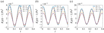
 Ha
 α=0.8
 β=0.2
 α=1
 β=0
 α=1
 β=1
 κ=10
 Re=5
 De=1
 ω=20
 ζ=0.5
 δ=0.01

 t
 α
 β
 κ=10
 Re=5
 De=1
 ω=20
 Ha=0.6
 ζ=0.5
 δ=0.01

 t
 δ
 ω=20
 ω
 δ=0.01
 κ=10
 De=1
 Re=5
 Ha=0.6
 ζ=0.5
 α=0.8
 β=0.4

 Pe=50
 κ=10
 Re=5
 De=1
 Ha=0.6
 ζ=0.5
 ω=20
 δ=0.01
 α=0.8
 β=0.4
 xs=0.019

 Pe=50
 κ=10
 Re=5
 De=1
 ω=20
 ζ=0.5
 δ=0.01
 α=0.8
 β=0.4
 xs=0.019

 Pe=50
 κ=10
 Re=5
 De=1
 ω=20
 ζ=0.5
 δ=0.01
 α=0.8
 β=0.4
 xs=0.019

 Pe=50
 κ=10
 Re=5
 De=1
 ω=20
 Ha=0.6
 ζ=0.5
 α=0.8
 β=0.4
 xs=0.019

 Pe=50
 Re=5
 De=1
 κ=10
 ω=20
 Ha=0.6
 ζ=0.5
 δ=0.01
 xs=0.019

 α
 β
 t=0.1
 α
 β
 Pe=50
 κ=10
 Re=5
 De=1
 ω=20
 δ=0.01
 Ha=0.6
 ζ=0.5
 xs=0.019

 Re
 α=0.8
 β=0.4
 Pe=50
 κ=10
 De=1
 ω=20
 Ha=0.6
 ζ=0.5
 δ=0.01
 xs=0.019

 De
 α=0.8
 β=0.4
 Pe=50
 κ=10
 Re=5
 ω=20
 Ha=0.6
 ζ=0.5
 δ=0.01
 xs=0.019

 ω
 Re=5
 α=0.8
 β=0.4
 Pe=50
 κ=10
 De=1
 Ha=0.6
 ζ=0.5
 δ=0.01
 xs=0.019

 t=0
 α
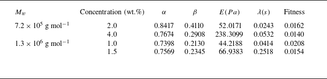

 G′
 G″
 Mw=7.2×10⁵
 gmol−1
 Mw=1.3×10⁶
 gmol−1


 G′
 G″


