2. Atlas and quasi-Atlas models

We use systems of strictly positive continuous semimartingales $\{X_1,\ldots, X_n\}$, with $n>1$, to approximate systems of time-dependent data. For such a system we define the rank function to be the random permutation $r_t\in\Sigma_n$, for $t\ge0$, such that $r_t(i)<r_t(j)$ if $X_i(t)>X_j(t)$ or if $X_i(t)=X_j(t)$ and $i<j$. Here, $\Sigma_n$ is the symmetric group on n elements. The rank processes $\{ X_{(1)}\ge\cdots\ge X_{(n)} \}$ are defined by $X_{(r_t(i))}(t)=X_i(t)$.

For a continuous semimartingale X, we can define the semimartingale local time at the origin $\Lambda_{}$ by the Tanaka–Meyer formula

\begin{equation*}\Lambda_{}(t)\triangleq \frac{1}{2}\Big(|X(t)|-|X(0)|-\int_0^t\text{sgn}(X(s))\,\textrm{d} X(s)\Big),\end{equation*}

for $t \geq 0$, where sgn$(x)=2\,\textbf{1}_{\{x>0\}}-1$, for $x\in{\mathbb R}$ (see [Reference Karatzas and Shreve30, (7.7)–(7.9), p. 220]). The local time $\Lambda_{}$ measures the amount of time that X spends near $0^+$. The mapping $t \mapsto \Lambda_{}(t)$ is continuous and nondecreasing, and induces the random measure $\textrm{d}\Lambda_{}$ with support contained in the set $\{t\ge0\,:\,X(t)=0\}$ (see [Reference Karatzas and Shreve30, Theorem 7.1(ii), p. 218]).

We have assumed that the semimartingales $X_i$ are strictly positive, so we can consider the logarithmic processes $\log X_1,\ldots,\log X_n$. For $1\le k< \ell \le n$, let $\Lambda_{k,\ell}^X$ denote the local time at the origin for $\log X_{(k)}-\log X_{(\ell)}$, with $\Lambda_{0,1}^X=\Lambda_{n,n+1}^X\equiv 0$. The processes $\log X_1,\ldots,\log X_n$ have a triple point at time $t>0$ if there exist $j<k<\ell$ such that $\log X_j(t)=\log X_k(t)=\log X_{\ell}(t)$. Multidimensional Brownian motion almost surely has no triple points (see [Reference Karatzas and Shreve30, Proposition 3.22, p. 161]), but some of the systems we consider satisfy only the weaker condition that the processes $\log X_1,\ldots,\log X_n$ accumulate no local time at triple points, by which we mean that, for all $\ell\ge k+2$, we have $\Lambda_{k,\ell}\equiv 0$, almost surely (a.s.). If the $\log X_i$ accumulate no local time at triple points, then [Reference Banner and Ghomrasni5, Theorem 2.5] shows that the rank processes $\log X_{(k)}$ satisfy

(2.1) \begin{equation}\textrm{d}\log X_{(k)}(t)=\sum_{i=1}^n\textbf{1}_{\{r_t(i)=k\}}\,\textrm{d}\log X_i(t)+\frac{1}{2} \textrm{d}\Lambda_{k,k+1}^X(t)-\frac{1}{2} \textrm{d}\Lambda_{k-1,k}^X(t),\quad\text{\textrm{a.s.}},\end{equation}

for $t\ge0$ and $k = 1, \ldots, n$.

Let us define the processes $X_{[k]} \triangleq X_{(1)}+\cdots+X_{(k)}$, for $k=1,\ldots,n$. The following lemma shows that the local time process $\Lambda_{k,k+1}^X$ measures the flow into and out of $X_{[k]}$.

Lemma 2.1. Let $X_1, \ldots, X_n$ be strictly positive continuous semimartingales that satisfy (2.1). Then

(2.2) \begin{equation}\frac{1}{2} X_{(k)}(t)\textrm{d}\Lambda_{k,k+1}^X(t)= \textrm{d} X_{[k]}(t)- \sum_{i=1}^n \textbf{1}_{\{r_t(i)\le k\}}\textrm{d} X_i(t),\quad\text{\textrm{a.s.}},\end{equation}

for $t\ge0$ and $k=1,\ldots,n$.

Proof. Suppose that the rank processes $X_{(k)}$ satisfy (2.1), so we have

\begin{equation*}\textrm{d}\log X_{(k)}(t) = \sum_{i=1}^{n} \textbf{1}_{\{r_t(i)=k\}}\textrm{d}\log X_i(t)+\frac{1}{2} \textrm{d}\Lambda_{k,k+1}^X(t)-\frac{1}{2} \textrm{d}\Lambda_{k-1,k}^X(t),\quad\text{\textrm{a.s.}},\end{equation*}

for $t\ge0$ and $k=1,\ldots,n$. By Itô’s rule this is equivalent to

\begin{align*}\frac{\textrm{d} X_{(k)}(t)}{X_{(k)}(t)}&= \sum_{i=1}^{n} \textbf{1}_{\{r_t(i)=k\}}\frac{\textrm{d} X_i(t)}{X_{i}(t)}+\frac{1}{2} \textrm{d}\Lambda_{k,k+1}^X(t)-\frac{1}{2} \textrm{d}\Lambda_{k-1,k}^X(t)\\ &= \sum_{i=1}^{n} \textbf{1}_{\{r_t(i)=k\}}\frac{\textrm{d} X_i(t)}{X_{(k)}(t)}+\frac{1}{2} \textrm{d}\Lambda_{k,k+1}^X(t)-\frac{1}{2} \textrm{d}\Lambda_{k-1,k}^X(t),\quad\text{\textrm{a.s.}},\end{align*}

for $t\ge0$ and $k=1,\ldots,n$. From this, we have

\begin{align*}\textrm{d} X_{(k)}(t) &= \sum_{i=1}^{n} \textbf{1}_{\{r_t(i)=k\}}\textrm{d} X_i(t)+\frac{1}{2} X_{(k)}(t)\textrm{d}\Lambda_{k,k+1}^X(t)-\frac{1}{2} X_{(k)}(t)\textrm{d}\Lambda_{k-1,k}^X(t)\\&= \sum_{i=1}^{n} \textbf{1}_{\{r_t(i)=k\}}\textrm{d} X_i(t)+\frac{1}{2} X_{(k)}(t)\textrm{d}\Lambda_{k,k+1}^X(t)-\frac{1}{2} X_{(k-1)}(t)\textrm{d}\Lambda_{k-1,k}^X(t),\quad\text{\textrm{a.s.}},\end{align*}

for $t\ge0$ and $k=1,\ldots,n$, since the support of $\textrm{d}\Lambda_{k-1,k}^X$ is contained in the set $\big\{t\,:\log X_{(k-1)}(t)=\log X_{(k)}(t)\big\}$. Now we can add up $\textrm{d} X_{(1)}(t)+\cdots+\textrm{d} X_{(k)}(t)=\textrm{d} X_{[k]}(t)$, and we have

\begin{equation*}\textrm{d} X_{[k]}(t)= \sum_{i=1}^{n} \textbf{1}_{\{r_t(i)\le k\}}\textrm{d} X_i(t)+\frac{1}{2} X_{(k)}(t)\textrm{d}\Lambda_{k,k+1}^X(t),\quad\text{\textrm{a.s.}},\end{equation*}

for $t\ge0$ and $k=1,\ldots,n$, and (2.2) follows.□

The local time process $\Lambda_{k,k+1}^X$ compensates for turnover into and out of the top k ranks. Over time, some of the higher-ranked processes will decrease and exit from the top ranks, while some of the lower-ranked processes will increase and enter those top ranks. Equation (2.2) measures the replacement of the top k ranks of the system by the lower ranks.

We are interested in systems that show stability by rank, at least asymptotically. Since we must apply our definition of stability to systems of empirical data as well as to continuous semimartingales, we use asymptotic time averages rather than expectations for our definitions. We shall show below that for the systems of continuous semimartingales we consider, a law of large numbers implies that the asymptotic time averages are equal to the corresponding expectations.

The simplest system we consider is an Atlas model, a system of strictly positive continuous semimartingales $\{X_1,\ldots,X_n\}$ defined by

(2.3) \begin{equation}\textrm{d}\log X_i(t) = -g\,\textrm{d} t+ng\textbf{1}_{\{r_t(i)=n \}}\textrm{d} t+\sigma\,\textrm{d} W_i(t),\end{equation}

for $t\ge0$ and $i=1,\ldots,n$, where $g>0$ and $\sigma>0$ are constants, and $(W_1, \ldots, W_n)$ is a Brownian motion (see [Reference Fernholz14, Example 5.3.3, p. 103]). Atlas models are asymptotically stable with parameters

(2.4) \begin{equation} \lambda_{k,k+1} = 2kg, \qquad \sigma^2_{k,k+1} =2 \sigma^2,\end{equation}

for $k = 1, \ldots, n-1$ (see [Reference Ichiba, Papathanakos, Banner, Karatzas and Fernholz29, Proposition 2]).

A modest generalization of the Atlas model is the first-order model, introduced in [Reference Fernholz14, Section 5.5]. A first-order model is a system of strictly positive continuous semimartingales $\{X_1,\ldots,X_n\}$ with

(2.5) \begin{equation}\textrm{d}\log X_i(t) = g_{r_t(i)}\,\textrm{d} t+G_n\textbf{1}_{\{r_t(i)=n\}}\textrm{d} t+\sigma_{r_t(i)}\,\textrm{d} W_i(t),\end{equation}

for $t\ge0$ and $i=1,\ldots,n$, where $\sigma^2_1,\ldots,\sigma^2_n$ are positive constants; $g_1,\ldots,g_n$ are constants that satisfy

(2.6) \begin{equation} g_1+\cdots+g_n \le 0 \quad\text{ and }\quad g_1+\cdots+g_k < 0 \text{ for } k < n;\end{equation}

$G_n=-(g_1 + \cdots + g_n)$; and $(W_1, \ldots, W_n)$ is a Brownian motion (see [Reference Banner, Fernholz and Karatzas4, (1.1)–(1.6)]). First-order models are asymptotically stable with parameters

(2.7) \begin{equation} \lambda_{k,k+1} = -2\big(g_1+\cdots+g_k\big), \qquad \sigma^2_{k,k+1} = \sigma_k^2+\sigma^2_{k+1}, \qquad\text{\textrm{a.s.}},\end{equation}

for $k = 1, \ldots, n-1$ (see [Reference Ichiba, Papathanakos, Banner, Karatzas and Fernholz29, Proposition 2]). Here we use a simple form of first-order model in which the drift parameters $g_k$ are constant and the variance parameters $\sigma^2_k$ grow linearly with rank. Accordingly, we define a quasi-Atlas model to be a first-order model determined by three parameters $g>0$ and $\sigma^2_2\ge\sigma^2_1>0$, such that

(2.8) \begin{equation}g_k = -g, \qquad \sigma^2_k = \sigma^2_1+(k-1)(\sigma^2_2-\sigma^2_1),\end{equation}

for $k=1,\ldots,n$. Hence, we see that Atlas models are a subclass of quasi-Atlas models, which in turn are a subclass of first-order models.

By [Reference Banner, Fernholz and Karatzas4, Proposition 2.3], each of the processes $X_i$ in a first-order model asymptotically spends equal time in each rank. Due to this ergodicity, the parameters ng in (2.3) and $G_n$ in (2.5) cause the asymptotic growth rate to be zero for each of the processes $\log X_i$, for $i=1,\ldots,n$. Equations (2.3) and (2.5) can be generalized by the addition of a term $\gamma\,\textrm{d} t$ on the right-hand side, where the constant $\gamma$ represents the common logarithmic growth rate of the system, but in our setting it is convenient to make the simplifying assumption that $\gamma=0$ (see, e.g., [Reference Banner, Fernholz and Karatzas4, (1.1) and (1.6)]). The condition (2.6), along with $G_n=-(g_1 + \cdots + g_n)$, stabilizes the system and prevents it from separating into smaller subsystems over time. A discussion of this stabilizing effect can be found in the Remark following Theorem 8 of [Reference Pal and Pitman35].

We see from (2.7) that for a first-order model the parameters $\lambda_{k,k+1}$ and $\sigma^2_{k,k+1}$ depend only on ranks 1 through $k+1$ and not on the number n of processes in the model. On a more intuitive level, the parameter $G_n$ is defined so that whatever the size n of the model, the ‘upward force’ $g_{k+1}+\cdots+g_n+G_n>0$ from below adjusts to counteract the ‘downward force’ $g_1+\cdots+g_k<0$ from above, with

\begin{equation*}g_{k+1}+\cdots+g_n+G_n=-(g_1+\cdots+g_k).\end{equation*}

The local time $\Lambda_{k,k+1}$ between ranks k and $k+1$ is determined by these upward and downward forces since they push these two ranks together, and the value of $\lambda_{k,k+1}$ depends on this local time.

Lemma 1 in [Reference Ichiba, Papathanakos, Banner, Karatzas and Fernholz29] shows that the processes $\log X_1,\ldots,\log X_n$ in a first-order model accumulate no local time at triple points. It is also known that a first-order model for which $k\mapsto\sigma^2_k$ is concave, i.e. for which $\sigma^2_{k+1}-\sigma^2_k\le\sigma^2_k-\sigma^2_{k-1}$, for $k=2,\ldots,n-1$, almost surely has no triple points, and this condition holds for Atlas and quasi-Atlas models [Reference Ichiba, Karatzas and Shkolnikov27, Reference Sarantsev36]. Hence, (2.1) and Lemma 2.1 are valid for Atlas and quasi-Atlas models.

For a first-order model $\{X_1,\ldots,X_n\}$, let us define the processes $\mathcal{X}_1,\ldots,\mathcal{X}_n$ by

\begin{equation*}\mathcal{X}_i(t)= \log X_i(t)-\frac{1}{n}\sum_{j=1}^n\log X_j(t),\qquad t\in[0,\infty),\end{equation*}

for $i=1,\ldots,n$, along with the corresponding ranked processes $\mathcal{X}_{(1)}\ge\cdots\ge \mathcal{X}_{(n)}$, with

\begin{equation*}\mathcal{X}_{(k)}(t)= \log X_{(k)}(t)-\frac{1}{n}\sum_{j=1}^n\log X_j(t),\qquad t\in[0,\infty),\end{equation*}

for $k=1,\ldots,n$. Then it follows from [Reference Ichiba, Papathanakos, Banner, Karatzas and Fernholz29, Proposition 1], [Reference Khas’minskii31, Theorems 3.1 and 3.2], or [Reference Khas’minskii32, Theorem 4.1], that $(\mathcal{X}_1,\ldots,\mathcal{X}_n)$, as a process with values in ${\mathbb R}^n$, has a unique stationary distribution. We define the gap processes by $\log X_{(k)}-\log X_{(k+1)}$, for $k=1,\ldots,n-1$, and the stationary distribution for $(\mathcal{X}_1,\ldots,\mathcal{X}_n)$ induces a stationary distribution for each gap process $\log X_{(k)}-\log X_{(k+1)}=\mathcal{X}_{(k)}-\mathcal{X}_{(k+1)}$ (see [Reference Ichiba, Papathanakos, Banner, Karatzas and Fernholz29, Corollary 2]).

For a first-order model $\{X_1,\ldots,X_n\}$, let $\xi_k$ represent the gap process $\log X_{(k)}-\log X_{(k+1)}$ in its stationary distribution, for $k=1,\ldots,n-1$. For an Atlas or quasi-Atlas model, the $\xi_k$ will be independent and exponentially distributed, so the stationary joint distribution of $(\xi_1,\ldots,\xi_{n-1})$ will be the product of the exponential marginal distributions (this follows from [Reference Harrison and Williams24, Theorem 9.2] and is a special case of [Reference Ichiba, Papathanakos, Banner, Karatzas and Fernholz29, Theorem 2]). It is also known that in this case $\xi_k$ has density function $\alpha_k \textrm{e}^{-\alpha_k x}$, for $x\in[0,\infty)$, with rate parameter

(2.9) \begin{equation}\alpha_k= \frac{2\lambda_{k,k+1}}{\sigma^2_{k,k+1}} \end{equation}

and expectation

\begin{equation*}{\mathbb E}\big[\xi_k\big]=\frac{1}{\alpha_k}=\frac{\sigma^2_{k,k+1}}{2\lambda_{k,k+1}}\end{equation*}

(see [Reference Ichiba, Papathanakos, Banner, Karatzas and Fernholz29, Theorem 2]). For $k=1,\ldots,n-1$, if $f\,:\,[0,\infty)\to{\mathbb R}$ is a measurable function with

\begin{equation*}\int_0^\infty |f(x)|\textrm{e}^{-\alpha_k x} \, \textrm{d} x<\infty,\end{equation*}

then the strong law of large numbers,

\begin{equation*}\lim_{T\to\infty}\frac{1}{T}\int_0^T f\big(\log X_{(k)}(t)-\log X_{(k+1)}(t)\big)\textrm{d} t={\mathbb E}\big[f(\xi_k)\big],\qquad\text{\textrm{a.s.}},\end{equation*}

holds (see [Reference Ichiba, Papathanakos, Banner, Karatzas and Fernholz29, Proposition 1], [Reference Khas’minskii31, Theorem 3.1], or [Reference Khas’minskii32, Theorem 5.1]). It follows from this that

(2.10) \begin{equation} \lim_{T\to\infty}\frac{1}{T}\int_0^T\big(\log X_{(k)}(t) - \log X_{(k+1)}(t)\big)\,\textrm{d} t = {\mathbb E}\big[\xi_k\big]=\frac{1}{\alpha_k}=\frac{\sigma^2_{k,k+1}}{2\lambda_{k,k+1}},\quad\text{\textrm{a.s.}},\end{equation}

and

(2.11) \begin{equation} \lim_{T\to\infty}\frac{1}{T}\int_0^T\frac{X_{(k+1)}(t)}{X_{(k)}(t)}\textrm{d} t={\mathbb E}\big[\textrm{e}^{-\xi_{k}}\big]=\frac{\alpha_k}{\alpha_{k}+1},\qquad\text{\textrm{a.s.}},\end{equation}

for $k=1, \ldots, n-1$ (see [Reference Ichiba, Papathanakos, Banner, Karatzas and Fernholz29, Theorem 1]).

For a first-order model $\{X_1,\ldots,X_n\}$, the asymptotic slope of the tangent to the log–log plot of the $X_{(k)}$ versus rank will be

(2.12) \begin{equation} \lim_{T\to\infty}\frac{1}{T}\int_0^T \frac{\log X_{(k)}(t) - \log X_{(k+1)}(t)}{\log(k) - \log(k+1)} \, \textrm{d} t\end{equation}

at rank k, so if we define the slope parameters $s_k$ by

(2.13) \begin{equation} s_k \triangleq k\lim_{T\to\infty}\frac{1}{T}\int_0^T \big(\log X_{(k)}(t) - \log X_{(k+1)}(t)\big) \, \textrm{d} t,\end{equation}

for $k = 1, \ldots, n-1$, then

(2.14) \begin{equation} -s_k\left(1 + \frac{1}{2k}\right) < \lim_{T\to\infty}\frac{1}{T}\int_0^T \frac{\log X_{(k)}(t) - \log X_{(k+1)}(t)}{\log(k) - \log(k+1)} \, \textrm{d} t < -s_k,\end{equation}

for $k = 1, \ldots, n-1$. Accordingly, for large enough k, the slope parameter $s_k$ will be approximately equal to minus the slope given in (2.12). For expositional simplicity, we treat the $s_k$ as if they measured the true log–log slopes between adjacent ranks, but it is important to remember that this equivalence is only as accurate as the range of the inequalities in (2.14).

For an Atlas model, it follows from (2.4), (2.10), and (2.13) that

(2.15) \begin{equation}s_k = \frac{\sigma^2}{2g},\qquad\text{\textrm{a.s.}},\end{equation}

for $k=1,\ldots,n-1$, so the stationary distribution of an Atlas model follows a Pareto distribution, at least within the approximation (2.14), and when $\sigma^2= 2g$ it follows Zipf’s law. For a quasi-Atlas model, we see from (2.7) and (2.10) that the slope parameters will be

(2.16) \begin{equation}s_k = \frac{ k\big(\sigma_k^2+\sigma^2_{k+1}\big)}{2\lambda_{k,k+1}}= \frac{ \sigma_k^2+\sigma^2_{k+1}}{4g},\qquad\text{\textrm{a.s.}},\end{equation}

for $k=1,\ldots,n-1$, so the stationary distributions of quasi-Atlas models are not confined to the class of Pareto distributions.

It is convenient to consider families of first-order models that share the same parameters, and for this purpose we define a first-order family to be a sequence of constants $\{g_k,\sigma^2_k\}_{ k\in{\mathbb N}}$ with $g_1+\cdots+g_k < 0$ and $\sigma^2_k > 0$, for $k\in{\mathbb N}$. A first-order family generates a class of first-order models $\{X_1,\ldots,X_n\}$, each defined as in (2.5) with the common parameters $g_k$ and $\sigma^2_k$, for $k\in{\mathbb N}$, with $G_n=-(g_1+\cdots+g_n)$, for $n\in{\mathbb N}$. An Atlas family is a first-order family with $g_k=-g<0$ and $\sigma^2_k=\sigma^2>0$, for $k\in{\mathbb N}$. A quasi-Atlas family is a first-order family with $g_k=-g<0$ and $\sigma^2_k=\sigma_1^2+(k-1)(\sigma^2_2-\sigma^2_1)>0$, for $k\in{\mathbb N}$.

For a first-order family $\{g_k,\sigma^2_k\}_{k\in{\mathbb N}}$ we shall use the notation ${\mathbb E}_n$ to denote the expectation with respect to the stationary distribution for the system $\{\log(X_{(1)}/X_{(2)}), \ldots,$ $\log(X_{(n-1)}/X_{(n)})\}$ defined by that family. For Atlas and quasi-Atlas models it is useful to measure the expected values of the ranked processes $X_{(k)}$ relative to the value of the top process $X_{(1)}$, so we define the ranked weight ratios

(2.17) \begin{equation}R_k\triangleq {\mathbb E}_n\bigg[\frac{X_{(k)}(t)}{X_{(1)}(t)}\bigg],\end{equation}

for $k=1,\ldots,n$ and $t\ge0$. Since ${\mathbb E}_n$ assumes the stationary distribution, and since the definition does not depend on weights below the kth rank, the ranked weight ratios are independent of both t and n. With the system in its stationary distribution, the random variables $\log(X_{(k)}(t)/X_{(k+1)}(t))$ are independent, so

(2.18) \begin{equation}R_k={\mathbb E}_n\bigg[\frac{X_{(k)}(t)}{X_{(k-1)}(t)}\bigg]\cdot{\mathbb E}_n\bigg[\frac{X_{(k-1)}(t)}{X_{(k-2)}(t)}\bigg]\cdots{\mathbb E}_n\bigg[\frac{X_{(2)}(t)}{X_{(1)}(t)}\bigg],\end{equation}

for $2\le k\le n$ and $t\ge0$, where the terms on the right-hand side can be calculated in terms of (2.11). We can also define, for $n\in{\mathbb N}$,

(2.19) \begin{equation}R_{[n]}\triangleq{\mathbb E}_n\bigg[\frac{X_{[n]}(t)}{X_{(1)}(t)}\bigg] = R_1+\cdots+ R_n,\end{equation}

for $t\ge0$.

For an Atlas or quasi-Atlas family, the parameters $\sigma^2_{k,k+1}$, $\lambda_{k,k+1}$, $s_k$, and $R_k$ are defined uniquely for $k\in{\mathbb N}$ by (2.4), (2.8), (2.15), (2.16), and (2.17), as the case may be. Let us note that for a quasi-Atlas family the slope parameters $s_k$ and ranked weight ratios $R_k$ do not depend on the number of processes in the model as long as $n>k$, so a quasi-Atlas family defines a unique asymptotic distribution curve. Accordingly, these families will allow us to derive results about asymptotic distribution curves without repeatedly reciting the characteristics of individual models. Moreover, we only consider values derived from a first-order family when the models in the family are in their stationary distribution. Hence, for the Atlas and quasi-Atlas families we consider, we can calculate the values of the $s_k$ and $R_k$ directly from the parameters g, $\sigma^2_1$, and $\sigma^2_2$, and we can ignore the models themselves.

3. Zipfian Atlas models as approximations of empirical systems

In this section we first consider how empirical systems of time-dependent data can be approximated by first-order models. In the case that these first-order approximations are in fact Atlas or quasi-Atlas models, we show that it is likely that the empirical systems will follow Zipfian or quasi-Zipfian distributions.

Suppose that $\{Y_1,\ldots,Y_n\}$, for $n>1$, is an asymptotically stable system of strictly positive continuous semimartingales with rank function $\rho_t\in\Sigma_n$, for $t\ge0$, such that $\rho_t(i)<\rho_t(j)$ if $Y_i(t)>Y_j(t)$ or if $Y_i(t)=Y_j(t)$ and $i<j$. Let $\{Y_{(1)}\ge\cdots\ge Y_{(n)}\}$ be the corresponding rank processes with $Y_{(\rho_t(i))}(t)=Y_i(t)$. As in Definition 2.1, for the processes $Y_1\ldots,Y_n$ we can define the parameters

(3.1) \begin{equation}\begin{split}\boldsymbol{\lambda}_{k,k+1} &\triangleq \lim_{t\to\infty}\frac{1}{t}\Lambda_{k,k+1}^Y(t) >0,\qquad\text{\textrm{a.s.}},\\[3pt] \boldsymbol\sigma^2_{k,k+1}&\triangleq \lim_{t\to\infty}\frac{1}{t}\big\langle {\log Y_{(k)}-\log Y_{(k+1)}} \big\rangle_t >0,\qquad\text{\textrm{a.s.}},\end{split}\end{equation}

for $k=1,\ldots,n-1$.

Definition 3.1. (Fernholz [Reference Fernholz14]) Let $\{Y_1,\ldots,Y_n\}$ be an asymptotically stable system of strictly positive continuous semimartingales with parameters $\boldsymbol \lambda_{k,k+1}$ and $\boldsymbol \sigma^2_{k,k+1}$, for $k=1,\ldots,n-1$, defined by (3.1). Then the first-order approximation of $\{Y_1,\ldots,Y_n\}$ is the first-order model $\{X_1,\ldots,X_n\}$ with

(3.2) \begin{equation}\textrm{d}\log X_i(t) = g_{r_t(i)}\,\textrm{d} t+G_n\textbf{1}_{\{r_t(i)=n\}}\textrm{d} t+\sigma_{r_t(i)}\,\textrm{d} W_i(t),\end{equation}

for $t\ge0$ and $i=1,\ldots,n$, where $r_t\in\Sigma_n$ is the rank function for the $X_i$, the parameters $g_k$ and $\sigma_k$ are defined by

(3.3) \begin{equation}\begin{split}g_k &= \frac{1}{2} \boldsymbol \lambda_{k-1,k} - \frac{1}{2} \boldsymbol \lambda_{k,k+1} \qquad \text{for } k=2,\ldots,n-1;\\[3pt]g_1&=-\frac{1}{2}\boldsymbol \lambda_{1,2} , \qquad g_n =g_{n-1}\land0;\\[3pt]\sigma_k^2 &= \frac{1}{4}\big(\boldsymbol \sigma^2_{k-1,k}+\boldsymbol \sigma^2_{k,k+1}\big) \qquad \text{for } k=2,\ldots,n-1;\\[3pt]\sigma^2_1 &=\sigma^2_2+\big(\sigma^2_{2}-\sigma^2_{3}\big)\textbf{1}_{\{2\sigma^2_2>\sigma^2_3\}} , \qquad \sigma^2_n =\sigma^2_{n-1}+\big(\sigma^2_{n-1}-\sigma^2_{n-2}\big)\lor0;\end{split}\end{equation}

where $\sigma_k$ is the positive square root of $\sigma^2_k$, $G_n=-(g_1+\cdots+g_n)$, and $(W_1,\ldots,W_n)$ is a Brownian motion.

The parameters $g_1$, $g_n$, $\sigma^2_1$, and $\sigma^2_n$ in (3.3) were chosen to preserve the structure of Atlas and quasi-Atlas models. For the first-order model (3.2) with parameters (3.3), equation (2.7) implies that

(3.4) \begin{equation} \lambda_{k,k+1}=-2\big(g_1+\cdots+g_k\big)= \boldsymbol \lambda_{k,k+1},\qquad\text{\textrm{a.s.}},\end{equation}

for $k=1,\ldots,n-1$, and

\begin{equation*} \sigma^2_{k,k+1}=\sigma^2_k+\sigma^2_{k+1}= \frac{1}{4}\big(\boldsymbol \sigma^2_{k-1,k}+2\boldsymbol \sigma^2_{k,k+1}+\boldsymbol \sigma^2_{k+1,k+2}\big),\qquad\text{\textrm{a.s.}},\end{equation*}

for $k=2,\ldots,n-2$, so the $\sigma^2_{k,k+1}$ are a smoothed version of the $\boldsymbol \sigma^2_{k,k+1}$. Hence, the parameters for a first-order approximation are similar to those of the asymptotically stable system that it approximates. We would also like to have the stable distributions of the two systems $\{\log(X_{(1)}/X_{(2)}),\ldots,\log(X_{(n-1)}/X_{(n)})\}$ and $\{\log(Y_{(1)}/Y_{(2)}),\ldots,$ $\log(Y_{(n-1)}/Y_{(n)})\}$ be similar, with

\begin{align*} &\lim_{T\to\infty}\frac{1}{T}\int_0^T\big(\log X_{(k)}(t)-\log X_{(k+1)}(t)\big)\,\textrm{d} t \cong\\[3pt] &\qquad\qquad\qquad\qquad\qquad\qquad\lim_{T\to\infty}\frac{1}{T}\int_0^T\big(\log Y_{(k)}(t)-\log Y_{(k+1)}(t)\big)\,\textrm{d} t,\qquad\text{\textrm{a.s.}},\end{align*}

for $k=1,\ldots,n-1$. From (3.3) and (3.4) we see that if the system $\{Y_1,\ldots,Y_n\}$ is a quasi-Atlas model with parameters $\textbf{\textit{g}}_k$ and $\boldsymbol \sigma^2_k$, then the first-order approximation $\{X_1,\ldots,X_n\}$ will also be a quasi-Atlas model with the same parameters $g_k=\textbf{\textit{g}}_k$ and $\sigma^2_k=\boldsymbol \sigma^2_k$, for $k=1,\ldots,n$. In this case it follows from (2.10) that

\begin{align*} &\lim_{T\to\infty}\frac{1}{T}\int_0^T\big(\log X_{(k)}(t)-\log X_{(k+1)}(t)\big)\,\textrm{d} t =\\[3pt] &\qquad\qquad\qquad\qquad\qquad\qquad \lim_{T\to\infty}\frac{1}{T}\int_0^T\big(\log Y_{(k)}(t)-\log Y_{(k+1)}(t)\big)\,\textrm{d} t,\qquad\text{\textrm{a.s.}},\end{align*}

for $k=1,\ldots,n-1$, so the stable distributions of the two systems will be the same.

Lemma 2.1 shows that the parameters $\boldsymbol \lambda_{k,k+1}$ can be expressed as

(3.5) \begin{equation} \boldsymbol \lambda_{k,k+1}=\lim_{T\to\infty}\frac{2}{T} \int_0^T\bigg(\frac{\textrm{d} Y_{[k]}(t)}{Y_{(k)}(t)}-\sum_{i=1}^n \textbf{1}_{\{\rho_t(i)\le k\}}\frac{\textrm{d} Y_i(t)}{Y_{(k)}(t)}\bigg),\qquad\text{\textrm{a.s.}},\end{equation}

for $k=1,\ldots,n-1$, in which all the terms on the right-hand side of the equation are observable. In a similar fashion we can write

(3.6) \begin{equation} \boldsymbol \sigma^2_{k,k+1}=\lim_{T\to\infty}\frac{1}{T}\int_0^T \textrm{d}\big\langle {\log Y_{(k)}-\log Y_{(k+1)}} \big\rangle_t,\qquad\text{\textrm{a.s.}},\end{equation}

for $k=1,\ldots,n-1$. These two equations will allow us to define parameters equivalent to $\boldsymbol \lambda_{k,k+1}$ and $\boldsymbol \sigma^2_{k,k+1}$ for time-dependent systems of empirical data.

Suppose now that we have a time-dependent system $\{ Z_1(\tau), Z_2(\tau), \ldots \}$ of positive-valued data observed at times $\tau\in\{1, 2, \ldots, T\}$, where $T>1$. Let

(3.7) \begin{equation} N_\tau = \#\{Z_1(\tau),Z_2(\tau),\ldots\}\qquad \text{and} \qquad N=N_{1}\land\cdots\land N_{T},\end{equation}

where $\#$ represents cardinality. Let $\rho_\tau\,:\,{\mathbb N}\to{\mathbb N}$ be the rank function for the system $\{Z_1(\tau),Z_2(\tau),\ldots\}$ such that $\rho_\tau$ restricted to the subset $\{1,\ldots,N_\tau\}$ is the permutation with $\rho_\tau(i)<\rho_\tau(j)$ if $Z_i(\tau)>Z_j(\tau)$ or if $Z_i(\tau)=Z_j(\tau)$ and $i<j$, and for $i>N_\tau$, $\rho_\tau(i)=i$. We define the ranked values $\{Z_{(1)}(\tau)\ge Z_{(2)}(\tau)\ge\cdots\}$ such that $Z_{(\rho_\tau(i))}(\tau)=Z_i(\tau)$ for $i\le N_\tau$, and for definiteness we can let $Z_{(k)}(\tau)=0$ for $k>N_\tau$. With these definitions, we have $Z_{[k]}(\tau)=Z_{(1)}(\tau)+\cdots+Z_{(k)}(\tau),$ for $k=1,\ldots,N$ and $\tau\in\{1,2,\ldots,T\}$.

We can mimic the time averages (3.5) and (3.6) to define the parameters

(3.8) \begin{equation} \boldsymbol \lambda_{k,k+1} \triangleq\frac{2}{T-1}\sum_{\tau=1}^{T-1}\bigg(\frac{Z_{[k]}(\tau+1)-Z_{[k]}(\tau)}{Z_{(k)}(\tau)}-\sum_{i=1}^N \textbf{1}_{\{\rho_{\tau}(i)\le k\}}\frac{Z_i(\tau+1)-Z_i(\tau)}{Z_{(k)}(\tau)} \bigg) \end{equation}

and

(3.9) \begin{align}&\boldsymbol \sigma^2_{k,k+1} \triangleq \frac{1}{T-1}\sum_{\tau=1}^{T-1}\Big(\big(\log Z_{(k)}(\tau+1)-\log Z_{(k+1)}(\tau+1)\big)\nonumber\\ &\qquad\qquad\qquad\qquad\qquad\qquad\qquad\quad\qquad -\big(\log Z_{(k)}(\tau)-\log Z_{(k+1)}(\tau)\big)\Big)^2,\end{align}

for $k=1,\ldots,N-1$.

Definition 3.2. Suppose that $\{Z_1(\tau),Z_2(\tau),\ldots\}$, for $\tau\in\{1,2,\ldots,T\}$, with $T>1$, is a time-dependent system of positive-valued data with N, $\boldsymbol \lambda_{k,k+1}$, and $\boldsymbol \sigma^2_{k,k+1}$ defined as in (3.7), (3.8), and (3.9). The first-order approximation of $\{Z_1(\tau),Z_2(\tau),\ldots\}$ is the first-order family $\{g_k,\sigma^2_k\}_{ k\in{\mathbb N}}$ with

(3.10) \begin{equation}\begin{split}g_k &= \frac{1}{2} \boldsymbol \lambda_{k-1,k} - \frac{1}{2} \boldsymbol \lambda_{k,k+1} \qquad \text{for } k=2,\ldots,N-1;\\[3pt] g_1 &=-\frac{1}{2}\boldsymbol \lambda_{1,2} , \qquad g_k =g_{k-1}\land0\text{ for } k\ge N; \\[3pt] \sigma_k^2 &= \frac{1}{4}\big(\boldsymbol \sigma^2_{k-1,k}+\boldsymbol \sigma^2_{k,k+1}\big) \qquad \text{for } k=2,\ldots,N-1;\\[3pt] \sigma^2_1 &=\sigma^2_2+\big(\sigma^2_{2}-\sigma^2_{3}\big)\textbf{1}_{\{2\sigma^2_2>\sigma^2_3\}} , \quad \sigma^2_k =\sigma^2_{k-1}+\big(\sigma^2_{k-1}-\sigma^2_{k-2}\big)\lor0\text{ for } k\ge N.\end{split}\end{equation}

If the first-order model $\{X_1,\ldots,X_{N}\}$ defined by (3.2) with parameters (3.11) satisfies

(3.11) \begin{align} &\lim_{T\to\infty}\frac{1}{T}\int_0^T\big(\log X_{(k)}(t)-\log X_{(k+1)}(t)\big)\,\textrm{d} t \cong\nonumber\\ &\qquad\qquad\qquad\qquad\qquad\qquad\qquad\qquad \frac{1}{T}\sum_{\tau=1}^{T}\big(\log Z_{(k)}(\tau)-\log Z_{(k+1)}(\tau)\big), \end{align}

for $k =1,\ldots,N-1$, then we say that the system $\{Z_1(\tau),Z_2(\tau),\ldots\}$ is rank-based. If the system $\{Z_1(\tau),Z_2(\tau),\ldots\}$ is rank-based and the first-order model $\{X_1,\ldots,X_{N}\}$ defined by (3.2) with parameters (3.10) is a quasi-Atlas model, then it follows from (2.10) and (3.11) that

(3.12) \begin{equation} \frac{1}{T}\sum_{\tau=1}^{T}\big(\log Z_{(k)}(\tau)-\log Z_{(k+1)}(\tau)\big) \cong \frac{\boldsymbol \sigma^2_{k,k+1}}{2\boldsymbol \lambda_{k,k+1}},\end{equation}

for $k =1,\ldots,N-1$. In this case, the slope parameters for the first-order approximation apply to the distribution curve for the empirical system $\{Z_1(\tau),Z_2(\tau),\ldots\}$, and this motivates the next two definitions.

We see that, in terms of the parameters g and $\sigma^2$, an Atlas family is Zipfian if and only if $\sigma^2=2g$, in which case $\alpha_k=k$ in (2.9) and

(3.13) \begin{equation} R_k=\frac{k-1}{k}\cdot\frac{k-2}{k-1}\cdots\frac{1}{2}=\frac{1}{k},\end{equation}

as in (2.11) and (2.18). Since many empirical distributions are not Zipfian but rather quasi-Zipfian, we need to formalize this concept for first-order families.

Definition 3.4. A first-order family is quasi-Zipfian if its slope parameters $s_k$ are nondecreasing with $s_1 \leq 1$ and

\begin{equation*} \lim_{k\to\infty}s_k \geq 1,\end{equation*}

where this limit includes divergence to infinity. A time-dependent rank-based system is quasi-Zipfian if its first-order approximation is quasi-Zipfian.

For a quasi-Atlas family that is not an Atlas family, we see that in terms of the parameters g, $\sigma^2_1$, and $\sigma^2_2$ of (2.8), the family is quasi-Zipfian if and only if $\sigma^2_1+\sigma^2_2\le4g$.

By these definitions, a Zipfian system is also quasi-Zipfian. Because the slope parameters $s_k$ are approximately equal to minus the slope of a log–log plot of size versus rank, Definition 3.4 implies that a time-dependent rank-based system will be quasi-Zipfian if this log–log plot of its first-order approximation is concave with slope not steeper than $-1$ at the highest ranks and not flatter than $-1$ at the lowest ranks.

Zipf’s law originally referred to the frequency of words in a written language [Reference Zipf44], with the system $\{Z_1(\tau),Z_2(\tau),\ldots\}$, where $Z_i(\tau)$ represents the number of occurrences of the ith word in a language at time $\tau$. To measure the relative frequency of written words in a language it is not possible to observe all the written words in that language. Instead, the words must be sampled, where a random sample is selected (without replacement), and the frequency versus rank of this random sample is studied. For example, in Wikipedia [42] 10 million words in each of 30 languages were sampled and the resulting distribution curves were created. If the sample is large enough, the distribution of the sampled data should not differ materially from the distribution of the entire data set, at least for the higher ranks.

An advantage that arises from using sampled data is that it is possible to keep the total number of data in the sample constant over time. The total number of written words that appear in a language is likely to increase over time, and this increase could bias estimates of some parameters. Sampling the data will remove such a trend from the data, since a constant number of words can be sampled at each time. Accordingly, in all cases we shall assume that global trends have been removed from the data, either by sampling or by some other means of detrending.

Since we have assumed that we have a constant sample size or that the data have been detrended, the total count of our sampled data will remain constant, so

(3.14) \begin{equation} Z_1(\tau) + Z_2(\tau) + \cdots = \text{ constant},\end{equation}

for $\tau\in\{1,2,\ldots,T\}$, where in the case of the Wikipedia words the constant would be 10 million.

Suppose we have a time-dependent system of positive-valued data $\{Z_1(\tau),Z_2(\tau),\ldots\}$, for $\tau\in\{1, 2, \ldots, T\}$ with $T>1$, and we observe the top n ranks, for $1<n<N$, with N from (3.7), along with $Z_{[n]}(\tau)=Z_{(1)}(\tau)+\cdots+Z_{(n)}(\tau)$. Since the total value of the sampled data in (3.14) is constant, for large enough n it is reasonable to expect the relative change of the top n ranks to satisfy

(3.15) \begin{equation}\frac{Z_{[n]}(\tau+1)-Z_{[n]}(\tau)}{Z_{[n]}(\tau)}\cong 0,\end{equation}

for $\tau\in\{1, 2, \ldots, T-1\}$ as n becomes large, at least on average over time. This condition is essentially a ‘conservation of mass’ criterion for $\{Z_1(\tau),Z_2(\tau),\ldots\}$, in which the total ‘mass’ (3.14) of the system remains constant, at least on average over time. It is useful to normalize the values $Z_{(k)}(\tau)$ and $Z_{[n]}(\tau)$ by measuring them relative to the largest value $Z_{(1)}(\tau)$, in which case (3.15) becomes

\begin{equation*} \frac{1}{\big(Z_{[n]}(\tau)/Z_{(1)}(\tau)\big)}\frac{Z_{[n]}(\tau+1)-Z_{[n]}(\tau)}{Z_{(1)}(\tau)}\cong 0,\end{equation*}

for $\tau\in\{1, 2, \ldots, T-1\}$ as n becomes large, at least on average over time. For the first-order family $\{g_k,\sigma^2_k\}_{k\in{\mathbb N}}$, this expression allows us to use the ranked weight ratios $R_k$ and $R_{[n]}$ of (2.17) and (2.19), and motivates the following definition.

Definition 3.5. The first-order family $\{g_k,\sigma^2_k\}_{k\in{\mathbb N}}$ is conservative if, for $T>0$,

\begin{equation*} \lim_{n\to\infty}\frac{1}{ R_{[n]}} {\mathbb E}_n\bigg[\frac{1}{T}\int_0^T\frac{\textrm{d} X_{[n]}(t)}{X_{(1)}(t)}\bigg]= 0.\end{equation*}

For the system $\{Z_1(\tau),Z_2(\tau),\ldots\}$, for $\tau\in\{1, 2, \ldots, T\}$, the replacement of processes in the top $n<N$ ranks by processes in the lower ranks over the time interval $[\tau,\tau+1]$ is measured by

\begin{equation*}Z_{[n]}(\tau+1)-\sum_{i=1}^N\textbf{1}_{\{\rho_{\tau}(i)\le n\}}Z_i(\tau+1),\end{equation*}

or

\begin{equation*}\big(Z_{[n]}(\tau+1)-Z_{[n]}(\tau)\big)-\Bigg(\sum_{i=1}^N\textbf{1}_{\{\rho_{\tau}(i)\le n\}}\big(Z_i(\tau+1)-Z_i(\tau)\big)\Bigg).\end{equation*}

While some replacement from lower ranks is necessary, it seems reasonable to expect that the system will be ‘complete’ in the sense that, on average, the relative proportion of the mass that is replaced becomes arbitrarily small for large enough n, i.e. that

\begin{equation*} \frac{1}{Z_{[n]}(\tau)}\bigg(Z_{[n]}(\tau+1)-Z_{[n]}(\tau)-\sum_{i=1}^N\textbf{1}_{\{\rho_{\tau}(i)\le n\}}\big(Z_i(\tau+1)-Z_i(\tau)\big)\bigg)\cong 0,\end{equation*}

for $\tau\in\{1, 2, \ldots, T-1\}$ and large enough n. As in Definition 3.5, in terms of the first-order approximation of $\{Z_1(\tau),Z_2(\tau),\ldots\}$, this becomes

(3.16) \begin{equation} \frac{1}{ R_{[n]}} {\mathbb E}_n\Bigg[\frac{1}{T}\int_0^T\frac{\textrm{d} X_{[n]}(t)}{X_{(1)}(t)}-\frac{1}{T}\int_0^T\Bigg(\sum_{i=1}^N\textbf{1}_{\{r_{t}(i)\le n\}}\frac{\textrm{d} X_i(t)}{X_{(1)}(t)}\Bigg)\Bigg]\cong 0,\end{equation}

for $T>0$ and large enough n, where $N>n$ and $\{X_1,\ldots,X_N\}$ is a first-order model defined by $\{g_k,\sigma^2_k\}_{k\in{\mathbb N}}$. By Lemma 2.1, this is equivalent to

\begin{equation*}\frac{1}{ R_{[n]}} {\mathbb E}_n\bigg[\frac{1}{T}\int_0^T\frac{X_{(n)}(t)}{2X_{(1)}(t)}\textrm{d}\Lambda_{n,n+1}^X(t)\bigg]\cong 0,\end{equation*}

for $T>0$ and large enough n. Since

\begin{equation*} \lim_{T\to\infty}\frac{1}{T}\int_0^T \textrm{d}\Lambda_{n,n+1}^X(t)=\lambda_{n,n+1}=-2\big(g_1+\cdots+g_n\big),\qquad\text{\textrm{a.s.}},\end{equation*}

condition (3.16) corresponds to

\begin{equation*}\frac{1}{ R_{[n]}} {\mathbb E}_n\bigg[\frac{1}{T}\int_0^T-\big(g_1+\cdots+g_n\big)\frac{X_{(n)}(t)}{X_{(1)}(t)}\textrm{d} t\bigg]\cong 0,\end{equation*}

for $T>0$ and large enough n. Since ${\mathbb E}_n$ assumes the stationary distribution, this is equivalent to

\begin{equation*}-\big(g_1+\cdots+g_n\big)\frac{ R_n}{ R_{[n]}}\cong 0,\end{equation*}

for large enough n, and with $G_n=-\big(g_1+\cdots+g_n\big)$, we have the following definition.

Definition 3.6. The first-order family $\{g_k,\sigma^2_k\}_{ k\in{\mathbb N}}$ is complete if

\begin{equation*} \lim_{n\to\infty} \frac{G_n R_n}{ R_{[n]}}= 0.\end{equation*}

For an Atlas or quasi-Atlas family $G_n=ng$, so for these families completeness is equivalent to

\begin{equation*} \lim_{n\to\infty} \frac{n R_n}{R_{[n]}}= 0.\end{equation*}

The following two propositions show that conservation and completeness are the basis for the Zipfian nature of the distributions of many systems of time-dependent rank-based data.

Proof. For an Atlas model $\{X_1,\ldots,X_n\}$ with parameters $g>0$ and $\sigma>0$, Itô’s rule implies that

\begin{equation*}\textrm{d} X_i(t) = \bigg( \frac{\sigma^2}{2}-g+ng\textbf{1}_{\{r_t(i)=n\}}\bigg)X_i(t)\,\textrm{d} t+\sigma X_i(t)\,\textrm{d} W_i(t),\qquad\text{\textrm{a.s.}},\end{equation*}

for $t\ge0$ and $i = 1, \ldots, n$. Hence,

\begin{equation*}\textrm{d} X_{[n]}(t)=\bigg(\frac{\sigma^2}{2}-g\bigg)X_{[n]}(t)\,\textrm{d} t+ X_{[n]}(t) \, \textrm{d} M(t) +ngX_{(n)}(t)\,\textrm{d} t, \qquad\text{\textrm{a.s.}},\end{equation*}

for $t\ge0$, where M is a local martingale incorporating all of the terms $\sigma \,\textrm{d} W_i(t)$. From this we have, for $t\ge0$,

\begin{equation*}\frac{\textrm{d} X_{[n]}(t)}{X_{(1)}(t)} = \bigg(\frac{\sigma^2}{2}-g\bigg)\frac{X_{[n]}(t)}{X_{(1)}(t)}\,\textrm{d} t + \frac{X_{[n]}(t)}{X_{(1)}(t)} \,\textrm{d} M(t) + \frac{ngX_{(n)}(t)}{X_{(1)}(t)}\,\textrm{d} t, \qquad\text{\textrm{a.s.}},\end{equation*}

so, for $T>0$,

\begin{equation*}{\mathbb E}_n\bigg[\frac{1}{T}\int_0^T\frac{\textrm{d} X_{[n]}(t)}{X_{(1)}(t)}\bigg]= \bigg(\frac{\sigma^2}{2}-g\bigg) R_{[n]}+ng R_n,\end{equation*}

or

(3.17) \begin{equation}\frac{1}{ R_{[n]}} {\mathbb E}_n\bigg[\frac{1}{T}\int_0^T\frac{\textrm{d} X_{[n]}(t)}{X_{(1)}(t)}\bigg]= \frac{\sigma^2}{2}-g+\frac{ng R_n}{ R_{[n]}}.\end{equation}

If an Atlas family is conservative and complete, then as n tends to infinity the first and last terms of (3.17) converge to zero, so $\sigma^2/2g = 1$ and the family will be Zipfian.

If the Atlas family is Zipfian then $\sigma^2/2g=1$, in which case (3.13) holds, so $R_k=\frac{1}{k},$ and

\begin{equation*} R_{[n]}=\sum_{k=1}^n \frac{1}{k}=O(\log n).\end{equation*}

It follows that

\begin{equation*}\frac{ng R_n}{ R_{[n]}}=\frac{g}{O(\log n)},\end{equation*}

so the family is complete, and with $\sigma^2/2=g$ the right-hand side of (3.17) converges to zero as n tends to infinity. Hence, the left-hand side must also converge to zero, so the family is conservative.□

This proposition has a natural counterpart for quasi-Atlas families.

Proposition 3.2. If a quasi-Atlas family is conservative and complete with

(3.18) \begin{equation} \lim_{n\to\infty} R_{[n]} \ge 2,\end{equation}

then it is quasi-Zipfian.

Proof. Let $\{X_1,\ldots,X_n\}$ be a quasi-Atlas model with parameters $g,\sigma^2_1>0$ and $\sigma^2_2\ge\sigma^2_1$, such that $g_k=-g$ and $\sigma^2_k=\sigma^2_1+(k-1)(\sigma^2_2-\sigma^2_1)$, for $k=1,\ldots,n$. Itô’s rule implies that

\begin{equation*}\textrm{d} X_i(t) = \bigg( \frac{\sigma^2_{r_t(i)}}{2} - g+ng\textbf{1}_{\{r_t(i)=n\}}\bigg)X_i(t)\,\textrm{d} t+\sigma_{r_t(i)} X_i(t)\,\textrm{d} W_i(t),\qquad\text{\textrm{a.s.}},\end{equation*}

for $t\ge0$ and $i = 1, \ldots, n$, so

\begin{equation*}\textrm{d} X_{[n]}(t) = \sum_{k=1}^n X_{(k)}(t)\bigg(\frac{\sigma^2_k}{2}-g\bigg)\textrm{d} t + \textrm{d} M(t) +ngX_{(n)}(t)\,\textrm{d} t, \qquad\text{\textrm{a.s.}},\end{equation*}

for $t\ge0$, where M is a local martingale incorporating all of the terms $\sigma_{r_t(i)}X_i(t) \, \textrm{d} W_i(t)$. As with (3.17) above, for $T>0$,

\begin{equation*} \frac{1}{ R_{[n]}} E_n\bigg[\frac{1}{T}\int_0^T\frac{\textrm{d} X_{[n]}(t)}{X_{(1)}(t)}\bigg]= \frac{1}{ R_{[n]}} \sum_{k=1}^n R_k\bigg(\frac{\sigma^2_k}{2}-g\bigg)+\frac{ng R_n}{ R_{[n]}}.\end{equation*}

Since the family is conservative and complete, the first and last terms of this equation converge to zero as n tends to infinity, so

(3.19) \begin{equation} \lim_{n\to\infty}\Bigg(\frac{1}{ R_{[n]}} \sum_{k=1}^n R_k\frac{\sigma^2_k}{2g}\Bigg) =1.\end{equation}

Let us now show that (3.18) implies that $s_1\le1$. Since $0<\sigma^2_1\le\cdots\le\sigma^2_n$, (3.19) implies that

\begin{align*} 1& \ge \lim_{n\to\infty}\frac{1}{ R_{[n]}}\frac{\sigma_1^2}{2g}+ \lim_{n\to\infty} \Bigg(\frac{1}{ R_{[n]}} \sum_{k=2}^n R_k\frac{\sigma^2_2}{2g}\Bigg)\\ &=\lim_{n\to\infty}\frac{1}{ R_{[n]}}\frac{\sigma_1^2}{2g} +\bigg(1- \lim_{n\to\infty} \frac{1}{ R_{[n]}}\bigg)\frac{\sigma_2^2}{2g}\\& \ge \frac{1}{2} \frac{\sigma_1^2}{2g}+\frac{1}{2} \frac{\sigma_2^2}{2g}=s_1,\end{align*}

where the last inequality follows from (3.18).

We must now show that either $\lim_{k\to\infty}s_k\ge 1$ or the $s_k$ diverge to infinity. Since the $\sigma^2_k$ are nondecreasing, as k tends to infinity they must either converge to a finite value $\sigma^2>0$ or diverge to infinity. We see from (2.16) that if the $\sigma^2_k$ diverge to infinity, the same will be true for the $s_k$. If $\lim_{k\to\infty}\sigma^2_k=\sigma^2$ then $\lim_{k\to\infty}s_k=\sigma^2/2g$, and since the $\sigma^2_k$ are nondecreasing,

\begin{equation*}1= \lim_{n\to\infty}\Bigg(\frac{1}{ R_{[n]}} \sum_{k=1}^n R_k\frac{\sigma^2_k}{2g} \Bigg)\le \frac{\sigma^2}{2g}.\end{equation*}

It follows that $\lim_{k\to\infty}s_k\ge 1$. □

These two propositions seem remarkably simple. Many empirical systems can be at least roughly approximated by quasi-Atlas models, and conservation and completeness are properties that are almost universal in large time-dependent rank-based systems of empirical data. If these conditions are satisfied, then these two propositions show that Zipf’s law, or at least its quasi-Zipfian counterpart, will pertain. Perhaps it is this simplicity that leads to the universality of Zipf’s law for these systems.

4. Examples and discussion

Empirical time-dependent systems often behave like quasi-Atlas families, and in Example 4.1 below we consider one such system, the capitalizations of US companies (see Figures 1 and 2). The condition that the variance rates increase with rank seems natural; even in the original observation of [Reference Brown8] it would seem likely that the water molecules would have buffeted the smaller particles more vigorously than the larger ones. Below the top few ranks, the members of empirical time-dependent systems constantly drift among nearby ranks, and this could result in linearity of the $\sigma^2_k$, at least throughout the middle ranks. Whether the $g_k=-g$ for all k may be more problematic, but this appears to hold at least in Example 4.1, where we analyze actual data. Since we are usually observing the top part of a larger distribution, there is ‘leakage’ out of the system, characterized by the last term in (2.2), so the constant $-g$ may represent the universal draw toward extinction in time-dependent rank-based systems.

Figure 1:

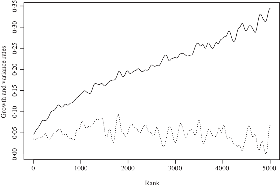
US capital distribution first-order parameters (smoothed): $\sigma^2_k$ (solid), $-g_k$ (dashed).

Figure 2:

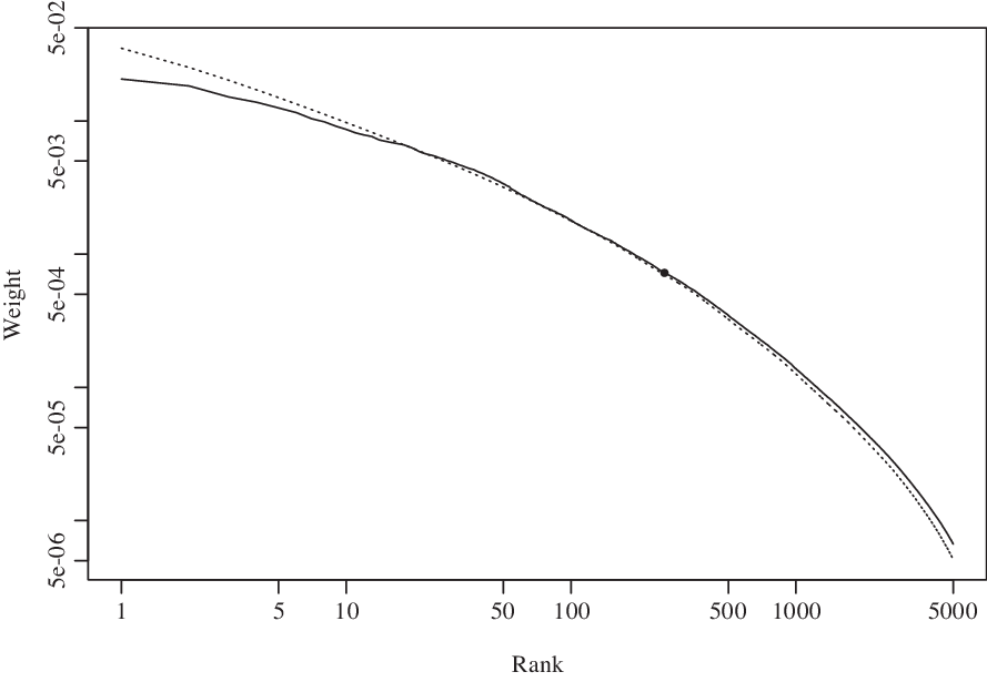
US capital distribution, 1990–1999 (solid). First-order approximation (dashed). The dot is the point at which the slope of the tangent is $-1$.

Figure 1 shows the smoothed first-order parameters $\sigma^2_k$ and $-g_k$ for the US capital distribution for the ten-year period from January 1990 to December 1999. The capitalization data we used were from the monthly stock database of the Center for Research in Securities Prices at the University of Chicago. The market we consider consists of the stocks traded on the New York Stock Exchange, the American Stock Exchange, and the NASDAQ Stock Market, after the removal of all Real Estate Investment Trusts, all closed-end funds, and those American Depositary Receipts not included in the S&P 500 Index. The parameters in Figure 1 correspond to the 5000 stocks with the highest capitalizations each month. The first-order parameters $g_k$ and $\sigma^2_k$ were calculated as in (3.10) from the parameters $\boldsymbol \lambda_{k,k+1}$ and $\boldsymbol \sigma^2_{k,k+1}$ of (3.8) and (3.9), and then smoothed by convolution with a Gaussian kernel with $\pm 3.16$ standard deviations spanning 100 months on the horizontal axis, with reflection at the ends of the data.

We see in Figure 1 that the values of the parameters $-g_k$ are relatively constant compared to the parameters $\sigma^2_k$, which increase almost linearly with rank. The near-constant $-g_k$ and near-linearly increasing $\sigma^2_k$ suggest that the first-order approximation can be represented by a quasi-Atlas family. In Figure 2, the distribution curve for the capitalizations is represented by the solid curve, which represents the average of the year-end capital distributions for the ten years spanned by the data. The dashed curve is the first-order approximation of the distribution following (3.12). The two curves are quite close, and this indicates that the time-dependent system of company capitalizations seems to be rank-based. The dot on the curve between ranks 100 and 500 is the point at which the log–log slope of the tangent to the curve is $-1$, so this is a quasi-Zipfian distribution, consistent with Proposition 3.2. Note that if we had considered only the top 100 companies, the completeness condition, Definition 3.6, would have failed, as we would expect for an incomplete distribution.

We can see from the remarkable chart in Wikipedia [42] that the log–log plots for 30 different languages are (almost) straight. Actually, these plots seem to be slightly concave, or quasi-Zipfian in nature. It is possible that this slight curvature is due to sampling error at the lower ranks, which would raise the variances and steepen the slope, but this would have to be determined by studying the actual data.

Example 4.3. (Random growth processes.) Economists have traditionally used random growth processes to model time-dependent systems with quasi-Zipfian distributions. For example, these processes were used in [Reference Gabaix21] to model the distribution of city populations and in [Reference Blanchet, Fournier and Piketty7] to construct a piecewise approximation to the distribution curves for the income and wealth of US households. A random growth process is an Itô process of the form

(4.1) \begin{equation}\frac{\textrm{d} X(t)}{X(t)}=\mu(X(t))\,\textrm{d} t+\sigma(X(t))\,\textrm{d} W(t),\end{equation}

for $t\ge0$, where W is Brownian motion and $\mu$ and $\sigma$ are well-behaved real-valued functions. We can convert this into logarithmic form by Itô’s rule, in which case

(4.2) \begin{equation}\textrm{d}\log X(t) = \bigg(\mu(X(t))-\frac{\sigma^2(X(t))}{2}\bigg)\textrm{d} t+\sigma(X(t))\,\textrm{d} W(t), \qquad\text{\textrm{a.s.}},\end{equation}

for $t\ge0$. We shall assume that this equation has at least a weak solution with $X(t)>0$, a.s., and that the solution has a stationary distribution.

Let us construct n independent and identically distributed copies $X_1,\ldots,X_n$ of X, all defined by (4.1) or, equivalently, by (4.2), and assume that the $X_i$ are all in their common stationary distribution. Let us assume that the $\log X_i$ accumulate no local time at triple points, so we can define the rank processes, and (2.1) and (2.2) will be valid. If the system is asymptotically stable we can calculate the corresponding rank-based growth rates $g_k$, but if we know the stationary distribution of the original process (4.1), then there is a simpler way to proceed.

If we know the common stationary distribution of the $X_i$, then we can calculate expectations under this stationary distribution and let

\begin{equation*} g_k= {\mathbb E}\bigg[\mu(X_{(k)}(t))-\frac{\sigma^2(X_{(k)}(t))}{2}\bigg] , \qquad \sigma^2_k= {\mathbb E}\big[\sigma^2(X_{(k)}(t))\big],\end{equation*}

for $t\ge0$ and $k=1,\ldots,n$. Under appropriate regularity conditions on the $\mu$ and $\sigma$, the expectations here will be equal to the asymptotic time averages of the functions. Since the $X_i$ are in their stationary distribution, the geometric mean $\big(X_1X_2 \ldots X_n\big)^{1/n}=\big(X_{(1)}X_{(2)}\ldots X_{(n)}\big)^{1/n}$ will also be in its stationary distribution, so for $t\ge0$,

\begin{equation*}\big(g_1+\cdots+g_n\big)t={\mathbb E}\big[\log \big(X_{(1)}(t)\cdots\ X_{(n)}(t)\big)-\log \big(X_{(1)}(0)\cdots\ X_{(n)}(0)\big)\big]=0.\end{equation*}

Hence, $g_1+\cdots+g_n=0$, with $g_1+\cdots+g_k<0$, for $k<n$, so the $g_k$ and $\sigma^2_k$ define the first-order model

(4.3) \begin{equation}\textrm{d}\log Y_i(t)= g_{r_t(i)}\textrm{d} t+\sigma_{r_t(i)}\textrm{d} W_i(t),\end{equation}

for $t\ge0$ and $i=1,\ldots,n$, where $W_1,\ldots,W_n$ is n-dimensional Brownian motion. In this case, $G_n=0$.

If the functions $\mu$ and $\sigma$ in (4.1) are smooth enough, then the system is likely to be rank based, with the stationary distribution of the first-order model (4.3) close to that of the original system (4.1). More conditions are required for this stationary distribution to be quasi-Zipfian, and to achieve a true Zipfian distribution, a lower reflecting barrier or other equivalent device must be included in the model [Reference Gabaix22].

There is another phenomenon that occurs with city size distributions. Suppose that rather than studying a large country like the US, we consider instead the populations of the cities in New York State. According to the 2010 US census, the largest city, New York City, had a population of 8 175 133, while the second largest, Buffalo, had only 261 310, so this distribution is non-Zipfian. The corresponding population of New York State was 19 378 102, so hypothesis (3.18) of Proposition 3.2 is satisfied, but nevertheless the proposition fails. This calls for an explanation, and we conjecture that while the population of the cities of New York State comprise a time-dependent system, this system is not rank based. The population of New York City is not determined merely by its rank among New York State cities, but is highly city specific in nature. Hence, we cannot expect the stationary distribution for the gap process between New York City and second-ranked Buffalo to be exponential, and we cannot expect the distribution of the system to be quasi-Zipfian.