1. Introduction
An aging population, greater longevity, earlier retirements, and a shift from defined benefit to defined contribution retirement plans are driving a renewed focus on determining how retirees should spend down their savings.Footnote 1 Despite known limitations, the most popular strategy calls for a constant real withdrawal of 4 percent each year of the household’s financial wealth at retirement.Footnote 2 That is, a household with $1 million in savings upon retirement makes a $40,000 withdrawal in the first year and inflation-adjusted withdrawals of $40,000 in subsequent years. The 4% rule originates from Bengen (1994), who finds that a retirement strategy with 50 percent in stocks, 50 percent in government bonds, and a 4 percent inflation-adjusted withdrawal rate survives each 30-year period in the US historical record from 1926 to 1991.Footnote 3 The ‘safe’ 4% spending rule is ubiquitous and recommended by financial advisors, brokerages, mutual fund companies, retirement groups, and the popular press. Choi (Reference Choi James2022) reviews the 50 most popular personal finance books and finds that, of the 12 providing explicit retirement spending advice, 7 recommend a 4 percent spending rule and 4 recommend an even higher rate (5%–8%). The 4% rule appears in congressional testimony and is detailed on multiple state and federal government websites.Footnote 4 Its ubiquity is also apparent in the growing Financial Independence Retire Early (FIRE) movement, wherein many millennials (22% according to a recent Vanguard survey) are planning for early retirement based on the 4% rule.Footnote 5
The 4% rule is a leading example of the divergence between finance theory and practice. Normative portfolio choice models often prescribe full, partial, or deferred annuitization of assets to address the risk of households outliving their wealth. In practice, however, few retirees purchase life annuities (Poterba, Venti, and Wise, Reference Poterba, Venti and Wise2011), and annuitization has, if anything, declined in popularity (Brown, Poterba, and Richardson, Reference Brown Jeffrey, Poterba and Richardson2023). Given retirees’ preference for spending rules over annuitization, the efficacy of spending rules is an important issue. Recent reviews by Choi (Reference Choi James2022) and Cochrane (Reference Cochrane John2022) emphasize the need to understand the gap between theory and practice and call for applications of portfolio theory that are accessible and useful to investors and policy makers. Our study adopts this approach. Obtaining reliable, quantitative evidence on the 4% rule and alternative withdrawal rates is of critical importance given their widespread use.Footnote 6
Retirees must balance the desire to make larger withdrawals to maintain a reasonable standard of living against two risks that can deplete their wealth: longevity risk (i.e., the retiree’s lifespan exceeds actuarial expectations) and return risk (i.e., poor real investment returns in retirement). Modeling the impact of a random US retiree’s longevity on withdrawal rules is straightforward given actuarial information on mortality risk. Modeling return risk is a more difficult problem. Quantifying the likelihood and severity of left-tail outcomes is particularly important, as poor market performance during retirement can be catastrophic. In the withdrawal rule literature, returns are typically modeled using either the historical performance of US asset classes or simulations parameterized to match the historical moments of US returns.
There are, however, reasons to be cautious when using historical US data to generate ex ante expectations of long-horizon investment outcomes and left-tail risk. A large literature identifies three primary concerns. First, the sample size of long-horizon returns for major asset classes in the US is exceedingly small. The commonly used post-1925 data on equity returns from the Center for Research in Security Prices (CRSP), for example, represent fewer than four independent observations of 30-year returns for US stocks. Overlapping observations do little to increase the effective sample size (Boudoukh, Israel, and Richardson, Reference Boudoukh, Israel and Richardson2019), so the US data provide limited statistical information about long-run asset performance. Second, the US data suffer from survivor bias (Brown, Goetzmann, and Ross, Reference Brown Stephen, Goetzmann William and Ross Stephen1995, Jorion and Goetzmann, Reference Jorion and Goetzmann William1999). That is, the design choice to formulate retirement advice using US data is influenced by the ex post success of the US financial markets, which is problematic for current and future retirees who are concerned with forward-looking performance. Third, the US sample is subject to an easy data bias (Dimson, Marsh, and Staunton, Reference Dimson, Marsh Paul and Staunton2002) as researchers focus on markets that, ex post, have uninterrupted return data that are not obfuscated by trading halts, wars, hyperinflation, and other extreme events. Consistent with the limitations of the US data, evidence suggests that (i) the historical US asset market performance exceeded ex ante expectations (see, e.g., Fama and French (Reference Fama Eugene and French Kenneth2002), Avdis and Wachter (Reference Avdis and Wachter Jessica2017); and Binsbergen, Hua, Peeters, and Wachter (Reference Binsbergen, Hua, Peeters and Wachter Jessica2024)) and (ii) the experience of US investors does not mirror that of investors in many other developed markets (see, e.g., Jorion and Goetzmann (Reference Jorion and Goetzmann William1999) and Anarkulova, Cederburg, and O’Doherty (Reference Anarkulova, Cederburg and O’Doherty2022)). For example, although long-horizon equity market losses are rare or non-existent in the US (e.g., Fama and French (Reference Fama Eugene and French Kenneth2018)), Japan’s stock market suffered a nominal (real) return of −9% (−21%) over the recent 30-year period from 1990 to 2019 (a period that began with Japan holding the top spot in the world in market capitalization). In sum, a substantial literature demonstrates that the historical record of asset-class performance in the US likely offers a poor reflection of the forward-looking return distribution.
In this study, we reevaluate the 4% rule for a US investor using a comprehensive new dataset of real returns for domestic equity, international equity, government bonds, and government bills in developed economies. The dataset is specifically constructed to combat the issues relating to small samples, survivor bias, and easy data bias that impact the conclusions of prior studies. The data cover approximately 2,500 years of asset-class returns in 38 developed countries over the period from 1890 to 2019. The long time-series and broad cross-sectional coverage yield a wealth of statistical information about potential investment outcomes and allow for a more complete characterization of left-tail risk. Our fundamental premise is that US investors today can form better ex ante expectations using a broad developed market sample free of survivor and easy data biases rather than relying on the small, biased US sample.
Using this dataset, we simulate retirement outcomes associated with alternative withdrawal rates. We model asset-class returns using a modification of the stationary block bootstrap of Politis and Romano (Reference Politis Dimitris and Romano Joseph1994) that maintains both cross-sectional and time-series properties of long-horizon asset returns. We incorporate longevity risk into the simulation design using mortality tables from the Social Security Administration (SSA). Our base case simulation focuses on the joint investment-longevity outcomes for a couple retiring in 2022 at age 65 who chooses a portfolio strategy of 60 percent domestic stocks and 40 percent bonds.
The 4% rule proves woefully inadequate for current retirees. A retired couple faces a 16.8 percent probability of depletion of financial wealth prior to death (henceforth, ‘financial ruin’) using the 4% rule, such that there is approximately a one-in-six chance that they must subsist – often for many years – solely on social welfare programs. Given the poor performance of the 4% rule, we explore alternative constant real withdrawal policies. Our findings suggest that most retirees (i.e., retirees with relatively modest levels of wealth) cannot achieve a reasonable standard of living while maintaining a very low ruin probability. To achieve a 1 percent ruin probability, for example, retirees must adopt a withdrawal rate of just 0.82 percent (i.e., $8,200 of withdrawals per year for $1 million in savings). When we attempt to balance the desires to achieve a higher standard of living and to avoid financial ruin, we find that a retired couple willing to bear a 5 percent ruin probability may withdraw 2.31 percent per year. This value is considerably lower than those proposed in prior studies, and it is just over half of the 4.26 percent rate implied by the post-1925 US data.
We consider three strategy modifications to assess the robustness of our results. First, we evaluate the impact of allowing investors to deviate from the base case allocation of 60 percent stocks and 40 percent bonds by investing more or less aggressively in stocks. In most specifications, these alternative investment strategies imply lower withdrawal rates relative to the static 60/40 stock-bond portfolio. The estimated withdrawal rates based on the developed country sample are also materially lower than those based on the US sample across all the allocation strategies considered. Second, we examine whether the investment strategies pursued by popular target-date funds are useful in supporting higher withdrawal rates. Target-date investment vehicles use glide-path strategies that shift into more conservative asset classes as the investor ages with the stated purposes of preserving wealth and mitigating longevity risk. We find, however, that target-date funds do little or nothing to enhance the modest withdrawals implied by our base case design. Moreover, target-date strategies underperform relative to the 60/40 stock-bond portfolio in terms of generating wealth for bequests. Third, we consider two alternative retirement spending approaches: (i) a ‘guardrails’ strategy that adjusts the payout rate as markets rise or fall and (ii) a constant payout rate of the current principal balance. Among potential spending rules, the 4% rule lies on one end of the spectrum given its rigid focus on maintaining constant real payouts at the risk of financial ruin, the constant percentage of wealth approach lies on the other end because it eliminates the risk of ruin by eschewing stability in real payouts, and the guardrails strategy lies between. Retirees who adopt any of these approaches fare significantly worse when judged using the developed market sample compared with using the US sample.
We also examine how future generations may fare as life expectancy increases. We use SSA mortality estimates for today’s young adults (retirement in 2065) and newborns (retirement in 2085) and find that the increased longevity materially impacts the safe withdrawal rate. For a retired couple willing to accept a 5 percent chance of financial ruin, the real withdrawal rate of 2.31 percent for today’s retirees drops to 2.06 percent for today’s young adults and to 1.98 percent for today’s newborns.
The underlying data for our base case results cover a broad cross section of 38 countries over a long sample period from 1890 to 2019. This approach invites potential concerns that the results are driven by historical asset market outcomes from periods that are less relevant for today’s investors or by countries with smaller and less developed economies compared with the US. We address these concerns by computing safe withdrawal rates from samples that include only post-World War II data or countries for which the market capitalization-to-GDP ratio has exceeded 0.5. The results for these restricted samples are close to those for the base case, with estimated real withdrawal rates at a 5 percent chance of financial ruin of 2.70 percent and 2.65 percent, respectively.
Although we define financial ruin as the retired couple depleting their savings, we recognize that most US retirees receive Social Security benefits (and a smaller, declining number receive income from defined benefit plans) that continue until death. But Social Security benefits for most retirees are modest.Footnote 7 The Social Security Administration advises retirees, ‘Social Security is not meant to be your only source of income in retirement. On average, Social Security will replace about 40 percent of your annual pre-retirement earnings ….’Footnote 8 As such, retirees who deplete their savings or who must substantially reduce their withdrawals are likely to face a poor standard of living.
Finally, we focus on spending rates for the US, but our results on safe withdrawal rates generalize to other developed countries. In fact, longevity is higher in most developed countries compared with the US. According to the World Bank, the current life expectancy is 76.3 years in the US versus 80.4 years in the European Union, such that current EU retirees have life expectancy (and safe withdrawal rates) similar to US newborns.Footnote 9 Of course, the degree of hardship associated with depleting financial wealth will also differ across countries due to differences in national retirement benefits and social programs.
The remainder of the paper is organized as follows. Section 2 provides background information on the withdrawal rule literature and measures to assess the performance of a given withdrawal plan. Section 3 describes our approach to constructing a sample of asset-class returns for a broad cross section of developed countries. Section 4 details our bootstrap methods for estimating the joint distribution of household portfolio and longevity outcomes. Section 5 presents our empirical findings, and Section 6 concludes.
2. Background
Nobel Laureate William Sharpe called the retirement wealth deaccumulation question the ‘nastiest, hardest problem in finance’ (Ritholtz, Reference Ritholtz2017). A retiree faces essentially three options for deaccumulation: (i) full annuitization, (ii) a phased withdrawal strategy (e.g., the 4% rule), or (iii) some combination of these two options (e.g., partial annuitization). Normative models typically conclude that most individuals should choose the first or third options. For instance, in a now classic study, Yaari (Reference Yaari1965) demonstrates that the optimal strategy for a retiree with no bequest motive is full annuitization of wealth at the onset of retirement. Davidoff, Brown, and Diamond (Reference Davidoff, Brown Jeffrey and Diamond Peter2005) reach a similar conclusion when relaxing many of the assumptions in Yaari (Reference Yaari1965). A growing body of work suggests that a combination strategy – either in the form of partial annuitization at retirement (known as a blended strategy) or a switching strategy (i.e., at some point moving from a phased withdrawal strategy to an annuitization strategy) – may be optimal (see, e.g., Dus, Maurer, and Mitchell (Reference Dus, Maurer Raimond and Mitchell Olivia2005), Horneff, Maurer, Mitchell, and Dus (Reference Horneff Wolfram, Maurer Raimond, Mitchell Olivia and Dus2008), Horneff, Maurer, Mitchell, and Stamos (Reference Horneff Wolfram, Maurer, Mitchell Olivia and Stamos Michael2010), Clare, Seaton, Smith, and Thomas (Reference Clare, Seaton, Smith Peter and Thomas2023); Estrada (Reference Estrada2017, Reference Estrada2018a, Reference Estrada2018b, Reference Estrada2018c); and Chen, Haberman, and Thomas (Reference Chen, Haberman and Thomas2023)).
Despite these normative conclusions, annuitization remains rare (Mitchell, Piggott, and Takayama, Reference Mitchell Olivia, Piggott and Takayama2011, Poterba, Venti, and Wise, Reference Poterba, Venti and Wise2011) and, if anything, has declined in popularity (Brown, Poterba, and Richardson, Reference Brown Jeffrey, Poterba and Richardson2023). A plethora of both rational explanations (e.g., precautionary savings for long-term care events, health risks, the implicit longevity insurance associated with Medicaid, unfair pricing of annuity contracts, bequest motives, within family pooling of longevity risk, and Social Security as an annuitization substitute) and behavioral explanations (e.g., framing effects, individuals’ inability to understand the value of an annuity, and confusion induced by too many choices) have been proposed to examine this ‘annuitization puzzle’. Brown (Reference Brown Jeffrey and Annamaria2009), Benartzi, Previtero, and Thaler (Reference Benartzi, Previtero and Thaler Richard2011), MacDonald, Jones, Morrison, Brown, and Hardy (Reference MacDonald, Jones, Morrison Richard, Brown Robert and Hardy2013); and Gomes, Haliassos, and Ramadorai (Reference Gomes, Haliassos and Ramadorai2021) provide excellent reviews of the annuitization puzzle.
2.1. Phased withdrawals
Most retirees choose to eschew annuitization and fund retirement income (other than Social Security and defined benefit income) from their retirement wealth. In these cases, a retiree faces uncertainty over both asset returns and her investment horizon and must make decisions related to the asset mix of her portfolio and the withdrawal rate. A retiree adopting an excessively high withdrawal rate increases her risk of running out of money in retirement, whereas one who chooses an excessively low rate faces a lower standard of living and an elevated ‘surplus risk’ (Suarez, Suarez, and Walz, Reference Suarez, Suarez and Walz2015) of living too frugally throughout retirement.
The research on phased withdrawals generally prescribes one of three methods: a constant fixed (typically inflation-adjusted) payout rate, a dynamic approach that adjusts the payout rate, or an optimization approach (e.g., lifetime utility maximization). The fixed approach, which includes Bengen’s (Reference Bengen William1994) seminal study, attempts to determine the asset mix and withdrawal rate that assure that the retiree can maintain the same real constant consumption with near certainty. As a result, the rate is denoted the safe withdrawal rate or the SAFEMAX rate. Scott, Sharpe, and Watson (Reference Scott Jason, Sharpe William and Watson John2009) argue, however, that a constant real withdrawal rate is ‘fundamentally flawed’ as the retiree has a surplus when markets do well, risks a shortfall if markets perform poorly, and does not maximize utility. The dynamic approaches may improve on the fixed approach by adjusting the payout based on portfolio performance, limiting inflation adjustments, recalculating withdrawal rates periodically, or recalculating the probability of financial ruin as the horizon changes (see, e.g., Bengen (Reference Bengen William2001), Pye (Reference Pye Gordon2001), Guyton and Klinger (Reference Guyton Jonathan and Klinger William2006), Spitzer (Reference Spitzer John2008), Blanchett and Frank (Reference Blanchett David and Frank Larry2009), Frank, Mitchell, and Blanchett (Reference Frank Larry, Mitchell John and Blanchett David2011), Zolt (Reference Zolt David2013), Suarez, Suarez, and Walz (Reference Suarez, Suarez and Walz2015); and Waring and Siegel (Reference Waring and Siegel Laurence2015)). Several related studies suggest that the appropriate withdrawal rate varies with market conditions such as overall market valuation levels (see, e.g., Finke, Pfau, and Blanchett (Reference Finke, Pfau Wade and Blanchett David2013), Blanchett, Buffenoir, Kemp, and Watt (Reference Blanchett, Buffenoir, Kemp and Watt2016), Clare, Seaton, Smith, and Thomas (Reference Clare, Seaton, Smith Peter and Thomas2017); and Arnott, Benz, and Rekenthaler (Reference Arnott, Benz and Rekenthaler2023)). Finally, several studies consider optimal withdrawal policies within a utility maximization framework (see, e.g., Horneff, Maurer, Mitchell, and Dus (Reference Horneff Wolfram, Maurer Raimond, Mitchell Olivia and Dus2008), Milevsky and Huang (Reference Milevsky and Huang2011), Blanchett, Kowara, and Chen (Reference Blanchett, Kowara and Chen2012), Habib, Huang, and Milevsky (Reference Habib, Huang and Milevsky Moshe2017); and Blanchett (Reference Blanchett2023)).
Despite the advances in more sophisticated dynamic or utility maximizing approaches, the 4% rule appears to remain the most popular approach in practice. For instance, a recent survey finds that 61 percent of advisors recommend their clients follow the 4% rule.Footnote 10 Each year Morningstar reports an updated estimate of the safe withdrawal rate (e.g., Arnott, Benz, and Rekenthaler (Reference Arnott, Benz and Rekenthaler2023)) that is widely followed in the popular press, and as noted in the introduction, the 4% rule is the standard recommendation in most popular personal finance books (Choi, Reference Choi James2022). The popularity of the 4% rule relative to more sophisticated approaches arises for at least three reasons. First, Blanchett (Reference Blanchett2023) posits that dynamic strategies have not been widely implemented in practice due to their complexity relative to fixed policies and the intricacies related to household heterogeneity. Second, the 4% rule is easy for clients to understand and for advisors to communicate (O’Connell, Edgar, Ormrod, Mussett, Benbow, and Prisk, Reference O’Connell, Edgar, Ormrod, Mussett, Benbow and Prisk2017). Third, recent survey evidence indicates that outliving their assets is a significant fear for many households.Footnote 11 Because the 4% rule is denoted the ‘safe’ withdrawal rate, the rule may (falsely) alleviate these fears even if it is not motivated via the traditional economic approach of utility maximization.
Most extant work estimates the safe withdrawal rate using one of three approaches: (i) backtests that rely on historical data (e.g., Bengen’s (Reference Bengen William1994) original study), (ii) Monte Carlo simulations (e.g., Cooley, Hubbard, and Walz (Reference Cooley Philip, Hubbard Carl and Walz Daniel2003a)), or (iii) analytical solutions based on assumed return distributions (e.g., Milevsky and Robinson (Reference Milevsky Moshe and Robinson2005) and Habib, Huang, and Milevsky (Reference Habib, Huang and Milevsky Moshe2017)). Regardless of the methodological approach, the vast majority of this work is based on historical US data (e.g., post-1925 Ibbotson data from the Stocks, Bonds, Bills and Inflation Yearbooks). There are, however, a few exceptions that incorporate non-US data. Cooley, Hubbard, and Walz (Reference Cooley Philip, Hubbard Carl and Walz Daniel2003b) find that international diversification improves the 4 percent payout success rate, whereas Ervin, Filer, and Smolira (Reference Ervin Danny, Filer Larry and Smolira Joseph2005) conclude that international diversification lowers the success rate. Blanchett, Buffenoir, Kemp, and Watt (Reference Blanchett, Buffenoir, Kemp and Watt2016) and Pfau (Reference Pfau Wade2010) consider other countries and find that the failure rate tends to be greater outside the US.Footnote 12 We also note that much existing work on the safe withdrawal rate focuses primarily on return uncertainty and assumes a fixed investment horizon (Stout and Mitchell (Reference Stout and Mitchell John2006) and Blanchett, Kowara, and Chen (Reference Blanchett, Kowara and Chen2012) are notable exceptions).
2.2. Financial ruin
Bengen’s (Reference Bengen William1994) original study proposes a fixed withdrawal rate that leads to zero ruin probability in historical 30-year periods of the US data. More recent work (e.g., Milevsky (Reference Milevsky2016), Bernhardt and Donnelly (Reference Bernhardt and Donnelly2018), Estrada and Kritzman (Reference Estrada and Kritzman2019); and Blanchett (Reference Blanchett2023)), however, highlights a number of limitations of focusing on the likelihood of financial ruin. For example, the probability of financial ruin ignores (i) the magnitude of the ruin event (e.g., running out of wealth in year 5 of a 30-year period is treated the same as running out of wealth in year 29), (ii) bequests, (iii) the ability of households approaching financial ruin to adjust spending, and (iv) heterogeneity in risk aversion. A number of studies overcome these issues by employing a risk-return or utility model (e.g., Dus, Maurer, and Mitchell (Reference Dus, Maurer Raimond and Mitchell Olivia2005), Horneff, Maurer, Mitchell, and Dus (Reference Horneff Wolfram, Maurer Raimond, Mitchell Olivia and Dus2008); and Horneff, Maurer, and Mitchell (Reference Horneff, Maurer and Mitchell Olivia2020, 2023)) or alternative measures that better capture the potential risks and rewards of a strategy (e.g., Blanchett (Reference Blanchett2007), Frank and Blanchett (Reference Frank Larry and Blanchett David2010), Blanchett, Kowara, and Chen (Reference Blanchett, Kowara and Chen2012), Suarez, Suarez, and Walz (Reference Suarez, Suarez and Walz2015), Clare, Seaton, Smith, and Thomas (Reference Clare, Seaton, Smith Peter and Thomas2017) Estrada (Reference Estrada2017, Reference Estrada2018a, Reference Estrada2018b, Reference Estrada2018c); and Estrada and Kritzman (Reference Estrada and Kritzman2019)).
Given the prior emphasis on of the probability of financial ruin throughout the academic literature and professional practice, our initial focus is on a comparison of the failure rates estimated from the US sample with those estimated from a broader sample of developed countries. This approach allows us to quantify the influence of small samples, survivor bias, and easy data bias on prior results. In our subsequent analyses, we consider alternative measures of the effectiveness of a given withdrawal plan. These measures capture distributional features of both the timing of failure and the magnitude of the household’s bequest. Although we focus on fixed withdrawal rates, we also evaluate more flexible approaches. The differences we document across the US and developed-country samples have important implications for all strategies – fixed withdrawals, flexible withdrawals, and annuitization.
3. Data
The primary data for our study are a panel of monthly real returns for domestic stocks, international stocks, bonds, and bills for 38 developed countries compiled by Anarkulova, Cederburg, and O’Doherty (Reference Anarkulova, Cederburg and O’Doherty2023). The data cover the period from 1890 to 2019, but as detailed below, the start dates for individual countries differ based on development classification and data availability. The sample construction is designed to mitigate two biases that plague other studies of investment performance in developed markets. First, a survivor bias (Brown, Goetzmann, and Ross, Reference Brown Stephen, Goetzmann William and Ross Stephen1995) arises if one conditions on eventual economic outcomes in sample construction. Second, an easy data bias (Dimson, Marsh, and Staunton, Reference Dimson, Marsh Paul and Staunton2002) follows from researchers’ preference to use readily available data that are uninterrupted by exchange closures accompanying wars, financial crises, and other extreme events. The Anarkulova, Cederburg, and O’Doherty (Reference Anarkulova, Cederburg and O’Doherty2023) dataset is specifically constructed to mitigate these biases by using ex ante measures of economic development to select markets, infilling incomplete data from historical sources, and carefully treating exchange closure periods.
3.1. Development classification
Developed countries are included in our sample following the development classification approach introduced in Anarkulova, Cederburg, and O’Doherty (Reference Anarkulova, Cederburg and O’Doherty2022). This approach mitigates survivor bias by relying on ex ante measures of economic development to determine the initial sample inclusion date for a given country. Prior to 1948, a country is added to the sample from the first year in which its labor share in agriculture drops below 50 percent. This classification method is motivated by evidence in the development economics literature that labor transitions from agriculture to manufacturing and services as an economy develops (see, e.g., Kuznets (Reference Kuznets1973)). Starting in 1948, a country is added to the sample from the year in which it joins the Organisation for Economic Co-operation and Development (OECD) or its predecessor, the Organisation for European Economic Co-operation (OEEC).
Table 1 (columns 2–3) shows the development year and classification benchmark for each country. With just three exceptions, each country remains in the sample through 2019 following its initial development classification. The exceptions correspond to Argentina (reclassified as a developing economy in 1966), Chile (1970), and Czechoslovakia (1945). In all three cases, the decision to reclassify the country follows substantial modifications to political and economic regimes.Footnote 13 Chile, the Czech Republic, and Slovakia ultimately reenter the sample based on admission to the OECD.
Developed country sample periods. The table shows developed countries, initial development dates, classification reasons for development, sample eligibility details, and sample coverage. The development year classifications are based on agricultural labor share or membership in the Organisation for European Economic Co-operation (OEEC) or the Organisation for Economic Co-operation and Development (OECD). Sample eligibility for a given developed country requires that the country has issued long-term government bonds. The sample period start date is the later of the eligibility date and the first date with return data for stocks, bonds, and bills. Coverage is the percentage of the eligible sample period with complete return data for a given country.

3.2. Asset-class returns
For each sample country, our panel of data contains monthly real returns on domestic stocks, international stocks, bonds, and bills over the developed period. The returns are measured in the local currency, and the local country’s inflation rate is used to adjust nominal returns to real returns. As such, the returns for a given country reflect the real investment outcomes of local investors.
The starting point for dataset construction is the GFDatabase from Global Financial Data. The GFDatabase contains long time series of total return indexes, price indexes, and dividend yields for stocks; yields for bonds and bills; consumer price indexes (CPIs); exchange rates; and total market capitalization for a broad set of countries. To mitigate easy data bias, Anarkulova, Cederburg, and O’Doherty (Reference Anarkulova, Cederburg and O’Doherty2022, 2023) undertake significant steps to clean and validate data, to fill in gaps in the GFDatabase using alternative sources (e.g., League of Nations reports, the St. Louis Federal Reserve, various central bank websites and statistical yearbooks for individual countries, and Jordà, Knoll, Kuvshinov, Schularick, and Taylor (Reference Jordà, Knoll, Kuvshinov, Schularick and Taylor Alan2019)), and to recreate the investor experience during major market disruptions. The authors also detail 35 historical instances in which stock exchanges close for extended periods and continuous monthly data are unavailable (e.g., the closure of the New York Stock Exchange in 1914 at the onset of World War I), and they construct monthly returns across these episodes to reflect economic outcomes for investors. The international stock returns for a given country are a market-capitalization-weighted investment in all non-domestic equity markets, and the return measurement incorporates exchange rate changes to capture currency risk. The bond returns are based on 10-year government bonds and reflect instances of sovereign default or bond exchange during the sample (e.g., the Greek default in 2012). The bill returns are primarily based on three-month government bills (with central bank rates, interbank rates, and other short-term interest rates filling occasional gaps in the data). We refer readers to Anarkulova, Cederburg, and O’Doherty (Reference Anarkulova, Cederburg and O’Doherty2022, 2023) for details on return measurement, special data issues, and dataset validation.
Table 1 provides details on sample eligibility (columns 4–5) and sample coverage (columns 6–8) for each developed country period. All country-months that are included in the sample have valid returns for all four asset classes. The eligible sample period represents the ideal period over which we would have complete return data. For most countries, sample eligibility starts from the later of 1890 (i.e., the start of the paper’s sample period) and the development classification year. We also require that a country has issued 10-year government bonds, and this requirement delays sample eligibility for nine countries.Footnote 14 The sample coverage results suggest that Anarkulova, Cederburg, and O’Doherty’s (Reference Anarkulova, Cederburg and O’Doherty2023) approach to data construction achieves comprehensive representation of the full developed period. Of the 39 developed country periods (i.e., 38 developed countries with two developed periods for Chile), our dataset contains a full time series of monthly data for all four asset classes for 27 cases. In the remaining cases, any missing observations occur at the beginning of the country’s sample, such that there are no unintentional data gaps in the middle or at the end of a given series. This feature is important for mitigating the impact of survivor and easy data biases. In total, we have complete data on domestic stocks, international stocks, bonds, and bills for 29,919 months of the 33,007 possible months, such that our dataset covers 91 percent of the eligible sample.
Table 2 reports the geometric mean and standard deviation of real returns for each sample country and for the pooled sample of all country-month observations. Although sample period differences cloud cross-country comparisons of asset-class returns, the US earns higher average domestic stock returns but lower average bond returns relative to most other countries. The US is not, however, an outlier based on average domestic stock or bond performance.
Summary statistics. The table reports summary statistics for monthly real returns for domestic stocks, international stocks, bonds, and bills for each developed country and for the pooled sample of all developed countries. The table shows the number of sample months (Obs) for each country and the geometric mean return (Mean) and the standard deviation of return (StDev) for each country and asset class.

3.3. Mortality
Our modeling approach examines the joint distribution of longevity and portfolio outcomes for US retirees. We model mortality risk using the period life tables from the SSA.Footnote 15 Table 3 summarizes the distribution of remaining life expectancy in years for the last survivor from a 65-year-old heterosexual couple at various retirement dates. Our base case scenario is investors retiring in 2022. The remaining life expectancy is 24.3 years for the last survivor, but there is considerable uncertainty about longevity outcomes. The 5th percentile of time to death is 12.2 years, whereas the 95th percentile is 34.5 years. The table also shows distributional statistics for investors retiring in 2065 (young adults today) or 2085 (newborns today). The life expectancies are longer, such that longevity concerns are more acute for younger generations.
Distribution of time to death. The table summarizes the distribution of remaining life expectancy in years of the last survivor from a 65-year-old heterosexual couple at various retirement dates. The distributions are constructed using the actuarial life tables from the Social Security Administration.

4. Methods
We use a Monte Carlo simulation approach to study portfolio outcomes as a function of the real withdrawal rate. Each draw from the simulation tracks the retirement account balance of a heterosexual couple from retirement at age 65 through death of the last survivor. We simulate portfolio outcomes using a stationary block bootstrap approach (Politis and Romano, Reference Politis Dimitris and Romano Joseph1994), in which the underlying data are the real returns on domestic stocks, international stocks, bonds, and bills for developed countries described in Section 3.2. We simulate longevity outcomes for the couple using the SSA mortality data described in Section 3.3.
Two aspects of the bootstrap procedure are particularly important for maintaining realistic aspects of the data. First, we draw matched sets of returns on domestic stocks, international stocks, bonds, and bills from the same country-months to preserve the cross-sectional relations across assets. Second, we draw blocks of returns that span many consecutive months from a given country using the block bootstrap to preserve time-series relations in the data. Block lengths are drawn from a geometric distribution with an average block length of 120 months. These long blocks allow the simulation to reflect short-term characteristics such as persistent return volatility and long-term characteristics like mean reversion in stock returns.
We consider outcomes for withdrawal rules ranging from 0 percent to 6 percent per year. Our base case uses the 2022 SSA life tables and portfolio weights of 60 percent domestic stocks and 40 percent bonds (henceforth the 60/40 portfolio). The 60/40 portfolio is a common investment rule of thumb, is consistent with the well-known home bias in asset holdings (see, e.g., French and Poterba (Reference French Kenneth and Poterba James1991)), and is a relatively successful investment allocation (as shown below). We also consider alternative simulation designs based on life expectancies for those retiring in 2065 or 2085; alternative stock-bond allocations ranging from 0 percent to 100 percent in stocks; allocations from a target-date fund that invests in domestic stocks, international stocks, bonds, and bills using a glide path that depends on the investor’s age; and alternative payout policies that deviate from fixed real withdrawal rules.
For each set of parameters, we generate 1,000,000 simulation draws to estimate financial ruin probabilities and other measures of interest. Each iteration  $m=1,\ldots, \mbox{1,000,000}$ has the following steps:
(1) We draw the remaining lifespans of a 65-year-old male, a 65-year-old female, and a couple (with lifespan equal to the greater of the male and female lifespans) using the SSA mortality tables. Mortality tables report death probabilities by age conditional on living until that age. Investors are assumed to retire when they turn 65. We use monthly conditional death probabilities and Bernoulli draws to determine whether death occurs in a given month. We convert the annual conditional death probabilities into monthly probabilities under the assumption of constant monthly death probabilities in a given year. We simulate the monthly longevity process until both the male and female have died, and we denote the length in months of the longer of the two lifespans as
 $T^{(m)}$.
(2) We draw monthly asset returns on domestic stocks, international stocks, bonds, and bills to form a time series of
$T^{(m)}$ months of returns using the stationary block bootstrap approach of Politis and Romano (Reference Politis Dimitris and Romano Joseph1994).(a) We draw a random block size b from a geometric distribution with a probability parameter equal to the inverse of the desired average block length (120 months).
(b) We randomly select a starting observation return vector for the block from the 29,919 country-month observations in the pooled sample. We denote this observation as
(1)$\begin{equation}
R_{i,t}=\left[R_{i,t}^{Domestic\ stocks} \qquad R_{i,t}^{International\ stocks} \qquad R_{i,t}^{Bonds} \qquad R_{i,t}^{Bills}\right],
\end{equation}$where i indexes the country and t indexes the month. The return block draw is
$B_b=\{R_{i,t}, R_{i,t+1}, \ldots, R_{i,t+b-1}\}$ if country i’s sample contains return observations
$R_{i,t}$ through
$R_{i,t+b-1}$. If not, then
$\{R_{i,t}, R_{i,t+1}, \ldots, R_{i,T}\}$, where
$R_{i,T}$ is the last observation in country i’s sample, is insufficient to fill block Bb. In this case, we draw a random country j from the 39 developed periods. If country j has enough observations to fill the remainder of the block, the block is
$B_b=\{R_{i,t}, R_{i,t+1}, \ldots, R_{i,T},R_{j,1},R_{j,2},\ldots,R_{j,b-(T-t+1)}\}$. If not, country j’s observations are added to the block, and we repeat the process and draw another random country until the block is filled.(c) We add Bb to the bootstrap return matrix draw
$R^{(m)}$. We return to step 2(a) and repeat the process until the return matrix has
$T^{(m)}$ months of data for the four assets. The final bootstrap draw in iteration m is
$R^{(m)}=\{R_1^{(m)},R_2^{(m)},\ldots,R_{T^{(m)}}^{(m)}\}$.
(3) We calculate the monthly retirement account balances through death of the last survivor of the couple. The retirement portfolio returns depend on the row vector of portfolio weights wt, where t indexes the month of the investor’s retirement period and wt contains weights for domestic stocks, international stocks, bonds, and bills. We consider seven sets of portfolio weights. Six of these seven maintain constant portfolio allocations across domestic stocks and bonds. We evaluate portfolio allocations of 100 percent bonds, 20 percent domestic stocks and 80 percent bonds, 40 percent stocks and 60 percent bonds, 60 percent stocks and 40 percent bonds, 80 percent stocks and 20 percent bonds, and 100 percent stocks. The seventh weighting scheme follows the glide path of a representative target-date fund, such that these weights change through retirement. Denoting the row vector of four asset returns in month t + 1 of retirement as
$R^{(m)}_{t+1}$, the portfolio return is
$R_{p,t+1}^{(m)}=R^{(m)}_{t+1}w_t^\prime$. Given initial wealth W 0 and adopted withdrawal rule r, the couple withdraws
$I=\frac{W_0r}{12}$ at the beginning of each month. Because all returns in our sample are real returns, this retirement income is expressed in real terms. Real retirement wealth evolves as
(2)\begin{equation}
W^{(m)}_{t+1}=\max(W_t^{(m)} - I,0)R^{(m)}_{p,t+1}.
\end{equation}Given the monthly retirement account balances, we calculate various quantities including a dummy variable for financial ruin (e.g.,
$W^{(m)}_{t+1}=0$ for
$t+1\leq T^{(m)}$), dummy variables for living for a certain number of months after financial ruin, and retirement wealth at death of the last survivor.


We use the Monte Carlo simulation to estimate probabilities of financial ruin, probabilities of outlasting retirement wealth and living a certain number of months, and quantiles of bequest ratios (i.e., ratios of real wealth at the time of death of the last survivor to real wealth at retirement) and coverage ratios by aggregating across the 1,000,000 draws for each set of parameter values. Following Estrada and Kritzman (Reference Estrada and Kritzman2019), the coverage ratio is defined as
 \begin{equation}
C^{(m)}=\left\{\begin{array}{ll} N^{(m)} / T^{(m)} & \text{for } N^{(m)} \lt T^{(m)}, \\ (T^{(m)} + W^{(m)}_{T^{(m)}} / I) / T^{(m)} & \text{for } N^{(m)} = T^{(m)}, \end{array}\right.
\end{equation}
where  $N^{(m)}$ is the number of months of positive withdrawals sustained by the strategy before the death of the last survivor. The coverage ratio is an appealing measure of strategy performance because it captures both the severity of financial ruin for couples who deplete their financial wealth before death and the bequest outcomes for couples who have remaining wealth at death. The coverage ratio is below one for couples who experience financial ruin, and the magnitude of the coverage ratio is the proportion of the retirement period over which the couple could consume from their retirement assets. For couples with positive wealth at death, in contrast, the coverage ratio is one plus the proportion of the retirement period spanned by additional withdrawals taken by their heirs.
5. Results
We examine joint investment-longevity results as a function of the real withdrawal rate. Our base case in Section 5.1 focuses on a retirement-age, US couple in 2022 who implements a portfolio allocation of 60 percent domestic stocks and 40 percent bonds. We consider alternative stock-bond weighting schemes in Section 5.2 and a target-date fund weighting scheme in Section 5.3. We examine retirement dates corresponding to younger investors in Section 5.4. We study alternative retirement withdrawal strategies in Section 5.5. Finally, we examine the robustness of our main findings to other sample formation screens in Section 5.6. For completeness, we report results for single retirees (i.e., 65-year-old females and males) in the appendix.
5.1. Base case
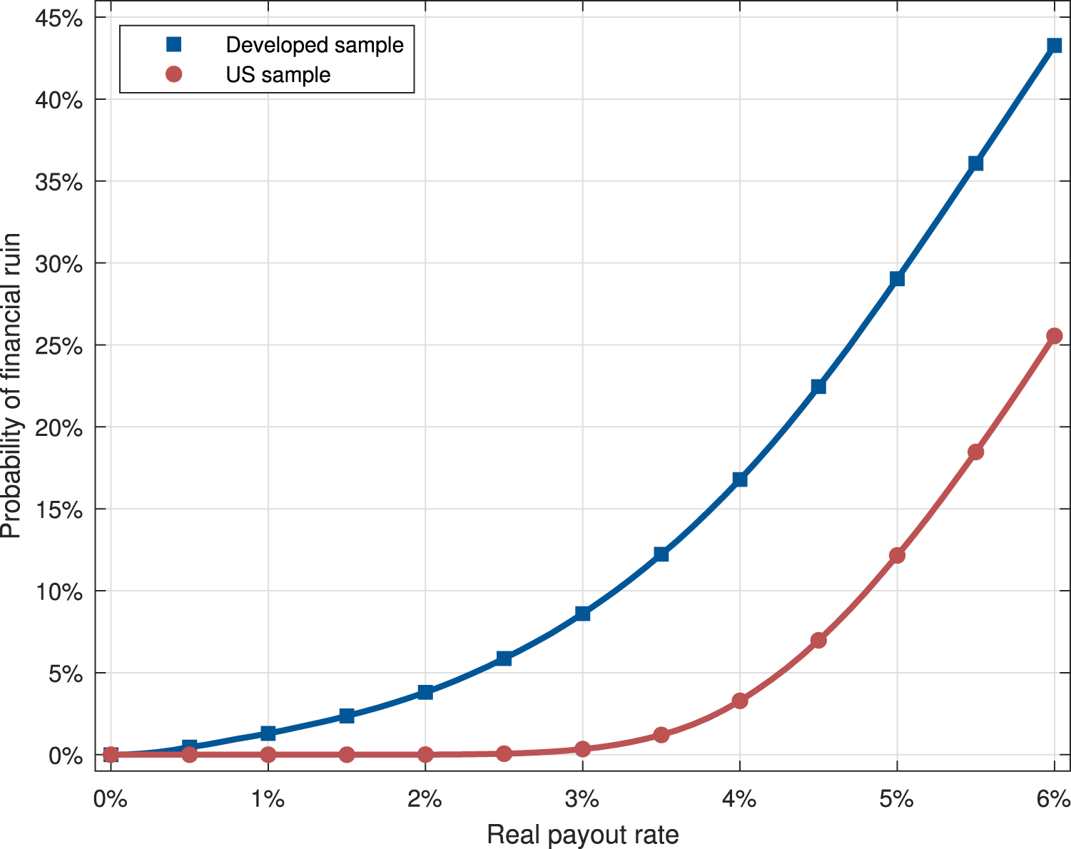
We begin our analysis with the base case of a 65-year-old couple in 2022 who holds the 60/40 portfolio. Figure 1 plots the likelihood that the couple fully depletes their retirement savings prior to the death of the last survivor (i.e., the probability of financial ruin) as a function of the real withdrawal rate. The blue line corresponds to our base case simulation design using the full sample of developed country returns. As a benchmark, the red line corresponds to a simulation that relies solely on the US data for the period from 1926 to 2019. The start of this US data series matches the start of the widely used CRSP data. Similar US-centric samples have been used extensively to calibrate inputs for retirement simulation exercises, but suffer from survivor and easy data biases. A comparison of the full-sample and US results yields quantitative evidence on the impact of these biases on retirement planning.
Probability of financial ruin. The figure plots the likelihood that a 65-year-old couple fully depletes their retirement wealth prior to the death of the last survivor as a function of the real withdrawal rate. The assumed asset allocation mix is 60% stocks and 40% bonds, and the survival probabilities are based on the 2022 actuarial life tables from the Social Security Administration. The blue (red) line shows the proportion of bootstrap simulations using the pooled sample of all developed countries (post-1925 US sample) in which wealth reaches zero prior to the death of the last survivor. We simulate 1,000,000 joint portfolio return and household survival outcomes for each combination of sample and withdrawal rate.

The simulation results suggest that Bengen’s (Reference Bengen William1994) original 4% rule exposes investors to considerable risk of outliving their wealth in retirement. The 4% rule leads to financial ruin in 16.8 percent of simulation runs. Bengen’s subsequently updated 5% rule has a failure rate of 29.0 percent, and even the more conservative 3.3% rule recently proposed by Benz, Ptak, and Rekenthaler (Reference Benz, Ptak and Rekenthaler2021) leads to a 10.7 percent probability of ruin.Footnote 16 Each of these failure rates likely exceeds a comfortable level of risk for most households.
In contrast, a model based on the historical US experience leads to a more encouraging view of the popular withdrawal plans. The failure rate for the 4% rule is 3.3 percent, and the failure rate for the 3.3% rule is just 0.8 percent. The results in Figure 1 thus highlight the pitfalls of using small historical samples and ignoring survivor and easy data biases in evaluating retirement withdrawal policies.
Because the most popular spending rules appear inadequate for facilitating a safe retirement when assessed relative to the broad developed country sample, we explore alternative withdrawal rates. Given the modest retirement savings balances for most households, we find that there is no withdrawal rate that both supports a reasonable consumption level and nearly assures that retirees will not outlive their wealth. We specifically estimate the level of accumulated savings required for a typical retired couple using a fixed withdrawal policy to meet their ‘basic needs’ and the level required to achieve a ‘reasonable standard of living’.
To obtain a quantitative estimate of basic needs, we consider data from the National Elder Economic Security Standard Index from the Gerontology Institute at the University of Massachusetts Boston. We estimate that the typical retired couple in 2023 needs annual income of at least $43,876 to cover ‘basic needs of elder households, including shelter, medical care, food, and transportation’.Footnote 17 As a proxy for a reasonable standard of living, we use Shrider, Kollar, Chen, and Semega’s (Reference Shrider Emily, Kollar, Chen and Semega2021) estimate of the median income in 2020 for US households ages 55–64 of $76,631.Footnote 18
Assuming that a given household receives the average annual Social Security benefit of $32,808, their savings balance at retirement would need to generate $11,068 (i.e., $43,876–$32,808) of annual income to meet basic needs and $43,823 (i.e., $76,631–$32,808) to maintain a reasonable standard of living equal to pre-retirement income. Using the 4% rule as an initial benchmark, the required retirement portfolio values for basic needs or no loss in income are, respectively, $0.28 million (i.e., $11,068/0.04) and $1.10 million (i.e., $43,823/0.04). Based on the evidence in Figure 1 for the developed country sample, however, retirees who are particularly concerned with mitigating the risk of financial ruin must accrue significantly larger account balances. Allowing for a 1 percent ruin probability, for example, implies a withdrawal rate of just 0.82 percent. This lower payout rate increases the required retirement portfolio size approximately fivefold to $1.35 million for the basic needs case and $5.34 million for the reasonable standard of living case.
Retirees are therefore faced with a tradeoff. Larger withdrawals enhance income and consumption, but smaller withdrawals alleviate the risk of financial ruin. To further characterize this tradeoff, we move away from ‘safe’ withdrawal rates and consider retirees who are willing to bear a higher risk of financial ruin. For example, Figure 1 shows that the withdrawal rate corresponding to a 5 percent failure probability estimated from the developed sample is 2.31 percent for couples retiring in 2022. The corresponding rate estimated from the US sample is 4.26 percent. The economic implications of the disparity in these rates are significant. To illustrate, consider a household seeking to maintain the $76,631 median income for US households ages 55–64. A 2.31 percent withdrawal rate implies that a couple receiving the average annual Social Security benefit needs $1.90 million in retirement savings rather than the $1.03 million implied by a 4.26 percent real payout rate.
To complement the evidence on the quantitative impact of our developed country dataset for safe withdrawal rates and the likelihood of financial ruin, we consider a series of other measures of fixed withdrawal strategy performance. Our broad-based developed country sample also has implications for projected wealth accumulation and bequests.Footnote 19 Figure 2 summarizes the distribution of the bequest ratio (i.e., real wealth at the time of death of the last survivor from the couple divided by real wealth at retirement) based on the developed sample (blue) and the US sample (red) as a function of the real withdrawal rate. For each sample, the solid line corresponds to the median bequest ratio, and the shaded region covers the 10th–90th percentiles of the ratio. Both samples suggest considerable uncertainty about real bequests. For a couple willing to bear a 5 percent probability of ruin (i.e., one with a 2.31 percent withdrawal rate), for example, the 10th percentile of the bequest ratio for the developed sample simulation is 0.25, whereas the 90th percentile is 5.27. The most pronounced feature of the plot, however, is the downward shift of the distribution based on the developed sample relative to the distribution based on the US sample. For instance, at a 4 percent withdrawal rate, the US data suggest that the median ending wealth to support bequests is 61 percent higher than starting retirement wealth. In contrast, the median ending wealth outcome is 9 percent lower than starting retirement wealth based on the developed sample.
Distribution of bequest ratio. The figure plots the distribution of the ratio of real ending wealth to real wealth at the start of retirement for a 65-year-old couple as a function of the real withdrawal rate. Real ending wealth is the real wealth at the time of death of the last survivor. The assumed asset allocation mix is 60% stocks and 40% bonds, and the survival probabilities are based on the 2022 actuarial life tables from the Social Security Administration. The blue (red) plot corresponds to the distribution of the bequest ratio across bootstrap simulations using the pooled sample of all developed countries (post-1925 US sample). The solid lines indicate the median bequest ratios, and the shaded regions covers the 10th–90th percentiles of the distributions. We simulate 1,000,000 joint portfolio return and household survival outcomes for each combination of sample and withdrawal rate.

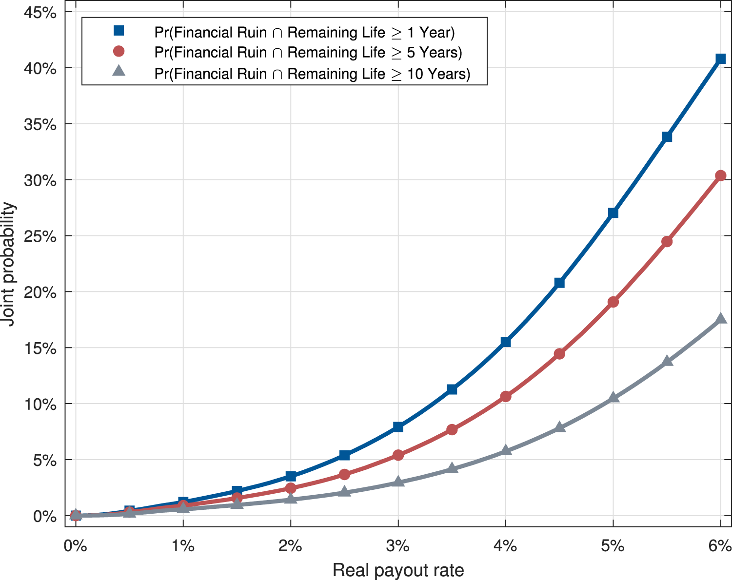
The implications of the elevated financial ruin probabilities estimated from the developed sample in Figure 1 are particularly acute if retirees experience ruin well before death. Figure 3 shows the joint probability (estimated from the developed sample) that a couple fully depletes their retirement wealth and the last survivor lives at least X additional years  $[X \in \{1,5,10\}]$ as a function of the real withdrawal rate. The results reveal that the economic consequences of adopting an overly aggressive withdrawal rate are severe. With the 4% rule, for example, there is a 15.5% (10.6%) [5.7%] chance that retirees will experience financial ruin and live one (five) [ten] or more years after exhausting their retirement wealth.
Remaining life upon financial ruin. The figure plots the joint likelihood that a 65-year-old couple fully depletes their retirement wealth prior to the death of the last survivor and the last survivor lives at least X additional years as a function of the real withdrawal rate. The assumed asset allocation mix is 60% stocks and 40% bonds. The survival probabilities are based on the 2022 actuarial life tables from the Social Security Administration, and the underlying sample for the bootstrap simulations is the pooled sample of all developed countries. The blue (red) [gray] line shows the joint probability of financial ruin and one member of the couple living at least one (five) [ten] years after ruin. We simulate 1,000,000 joint portfolio return and household survival outcomes for each withdrawal rate.

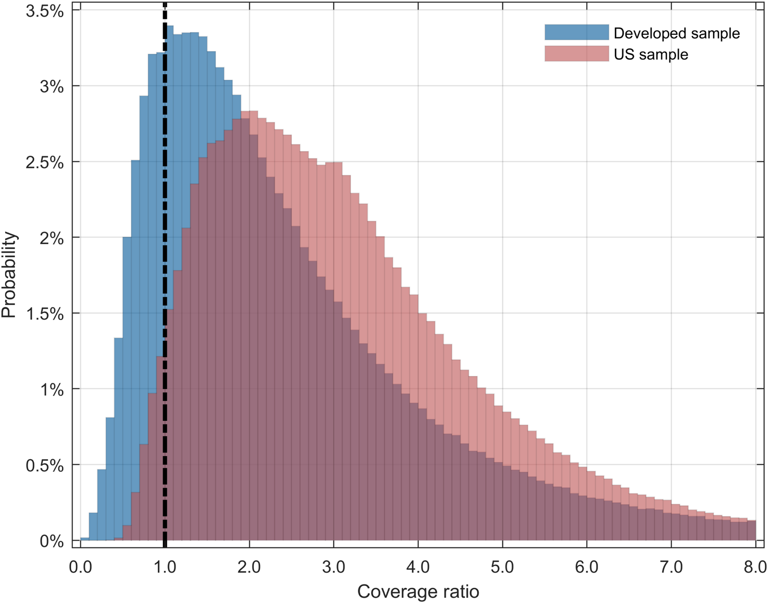
Finally, we compare the distribution of the coverage ratio defined in equation (3) from the perspective of investors using the developed sample to form their return expectations vis-à-vis those using the US sample. Figure 4 plots histograms of the realized coverage ratio based on simulations from the developed sample (blue) and the US sample (red) for households following the 4% withdrawal rule. As discussed in Section 4, the coverage ratio is a comprehensive measure of withdrawal strategy performance in that it reflects whether or not financial ruin occurs, the severity of the financial ruin event if it does occur, and the magnitude of the bequest if it does not. That is, a coverage ratio below one indicates that the household experiences financial ruin under the corresponding bootstrap draw and the magnitude of the coverage ratio in these cases is the proportion of the retirement period over which the retirement account supports withdrawals. For couples who die with positive retirement account balances to support bequests, the coverage ratio is greater than one and the value of the coverage ratio is one plus the proportion of the retirement period spanned by additional withdrawals.
Coverage ratio for the 4% rule. The figure plots histograms (normalized such that the total area equals 100%) of the coverage ratio (see equation (3)) for a 65-year-old couple following the fixed 4% withdrawal rule. The assumed asset allocation mix is 60% stocks and 40% bonds, and the survival probabilities are based on the 2022 actuarial life tables from the Social Security Administration. The blue (red) bars represent the distribution from a simulation using the pooled sample of all developed countries (post-1925 US sample). We simulate 1,000,000 joint portfolio return and household survival outcomes for each sample.

The results in Figure 4 highlight that the distribution of the coverage ratio estimated from the developed sample exhibits a pronounced shift to the left relative to the distribution estimated from the US sample. Households who form expectations of withdrawal strategy performance using the developed sample thus have considerably more pessimistic beliefs on the likelihood of exhausting their retirement assets before death, the severity of these ruin events, and the size of the bequests that they can leave to their heirs.
5.2. Alternative stock-bond allocation strategies
Our base case design focuses on the withdrawal policies of couples retiring in 2022 with a 60/40 portfolio. Panel A of Table 4 reports estimated withdrawal rates for ruin probabilities of 1 percent, 5 percent, and 10 percent based on the developed sample and the US sample for alternative stock-bond allocations. The table shows withdrawal rates for 2022 retiring couples with stock-bond allocations ranging from 0 percent stocks and 100 percent bonds to 100 percent stocks and 0 percent bonds; the results for 60 percent stocks and 40 percent bonds correspond to the base case from Section 5.1. The analysis yields no evidence that retirees can materially increase their withdrawal rates by shifting from the 60/40 portfolio to invest more heavily in stocks or bonds.Footnote 20 Moreover, the differences in results for the developed sample and the US sample suggest that accounting for survivor and easy data biases in financial asset returns remains important across all allocation strategies and tolerances for likelihood of financial ruin.
Withdrawal rates. The table shows the real payout rate in percentage estimated from 1,000,000 bootstrap simulations for various asset allocation strategies, retirement dates, and underlying data samples (i.e., the full sample of developed countries and the post-1925 US sample). The base case design (denoted with a  $\dagger$) corresponds to an asset allocation strategy of 60% stocks and 40% long-term bonds and a retirement date of 2022. The alternative cases modify the asset allocation strategy, the retirement date, or the data sample as described in the table. For each design, the table reports withdrawal rates corresponding to 1%, 5%, and 10% probabilities of financial ruin. The investor type is a heterosexual couple, such that financial ruin is defined as exhausting financial resources prior to death of the last survivor.

5.3. Target-date funds
Target-date funds (also known as life-cycle funds) have grown from approximately $900 billion in 2014 to $3.3 trillion in 2021 (Pacholok and Zaya, Reference Pacholok and Zaya2022), and more than half of 401(k) participants hold at least one target-date fund (Holden, VanDerhei, and Bass, Reference Holden, VanDerhei and Bass2021). A target-date fund implements a more aggressive portfolio when the investor is young to facilitate wealth accumulation. The strategy shifts toward a more conservative portfolio as the investor nears retirement age and typically becomes increasingly conservative through the retirement years with the intended purposes of preserving wealth and mitigating risks from longevity and poor investment performance.
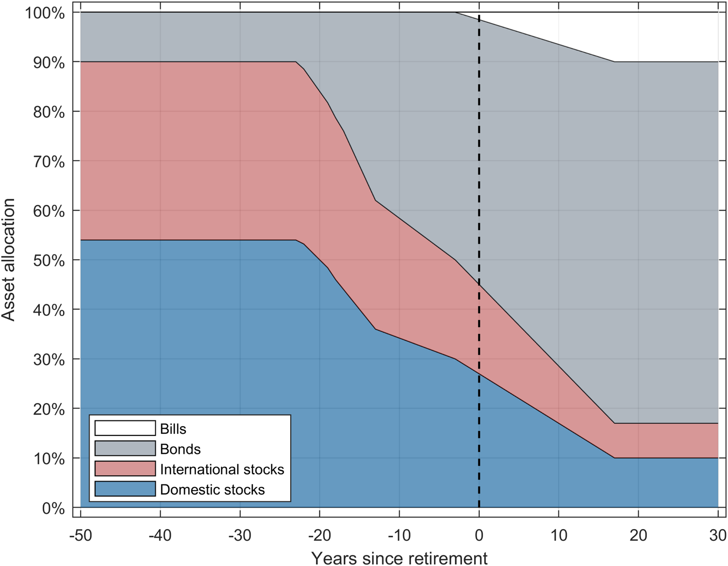
Figure 5 shows the glide-path weights for a representative target-date fund from a major investment advisor. During the investor’s early working years, the fund allocates 90 percent of the portfolio to domestic and international stocks and 10 percent to bonds. The stock weights begin to decrease about 20 years prior to the retirement date and continue to fall through the early retirement period. The allocation 30 years after the retirement date is 17 percent to domestic and international stocks and 83 percent to bonds and bills.
Target-date fund glide-path weights. The figure shows the approximate asset allocation of a representative target-date fund across domestic stocks, international stocks, bonds, and bills as a function of time since retirement.

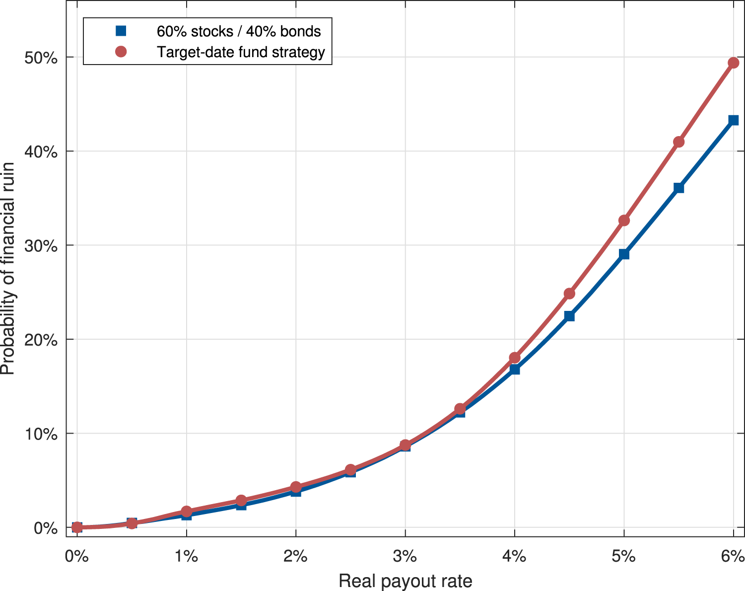
Panel B of Table 4 shows that the target-date strategy implies lower withdrawal rates compared with the 60/40 portfolio for failure probabilities of 1 percent, 5 percent, and 10 percent. For example, whereas our base case generates a 2.31 percent withdrawal rate for a 5 percent probability of ruin, the target-date strategy supports just 2.21 percent. This result generalizes. Figure 6 presents the probability of financial ruin as a function of the real withdrawal rate for the 60/40 and target-date fund strategies. The ruin probabilities are estimated using the developed sample for a couple retiring in 2022. The analysis offers no evidence that target-date funds support higher withdrawal rates by reducing longevity and return risks. The target-date strategy increases the likelihood of financial ruin relative to the 60/40 portfolio for each withdrawal rate in the relevant range.Footnote 21
Probability of financial ruin: Comparison of 60/40 strategy with target-date fund strategy. The figure plots the likelihood that a 65-year-old couple fully depletes their retirement wealth prior to the death of the last survivor as a function of the real withdrawal rate for alternative asset allocation strategies. The blue (red) line shows the probability of financial ruin for the investment strategy of 60% stocks and 40% bonds (the investment strategy implied by the glide path for a representative target-date fund). The survival probabilities are based on the 2022 actuarial life tables from the Social Security Administration, and the underlying sample for the bootstrap simulations is the pooled sample of all developed countries. We simulate 1,000,000 joint portfolio return and household survival outcomes for each combination of asset allocation strategy and withdrawal rate.

Figure 7 plots the distributions of the bequest ratio for the 60/40 strategy (blue) and the target-date strategy (red) based on the developed country sample. The solid lines denote median bequest ratios, and the shaded regions cover the 10th through 90th percentiles of bequest outcomes. The target-date strategy also performs poorly relative to the 60/40 portfolio in terms of wealth accumulation through retirement. The median and 90th percentile of the bequest ratio for the 60/40 portfolio are uniformly above the corresponding values for the target-date allocation, and the 10th percentiles of the two distributions are nearly identical. In short, our evidence suggests that target-date funds do not support higher withdrawal rates, considerably limit upside wealth accumulation for bequests, and fail to enhance downside protection.
Distribution of bequest ratio: Comparison of 60/40 strategy with target-date fund strategy. The figure plots the distribution of the ratio of real ending wealth to real wealth at the start of retirement for a 65-year-old couple as a function of the real withdrawal rate for alternative asset allocation strategies. Real ending wealth is the real wealth at the time of death of the last survivor. The blue (red) plot corresponds to the investment strategy of 60% stocks and 40% bonds (the investment strategy implied by the glide path for a representative target-date fund). The survival probabilities are based on the 2022 actuarial life tables from the Social Security Administration, and the underlying sample for the bootstrap simulations is the pooled sample of all developed countries. For each distribution, the solid line indicates the median bequest ratio and the shaded region covers the 10th–90th percentiles of the distribution. We simulate 1,000,000 joint portfolio return and household survival outcomes for each combination of asset allocation strategy and withdrawal rate.

5.4. Alternative retirement dates
The SSA predicts that life expectancies will increase over time. For example, Table 3 shows that the median remaining life expectancy for a couple retiring in 2085 is 15 percent longer than that for a couple retiring in 2022 (28.6 years versus 24.8 years). As a result, for any risk level the corresponding withdrawal rate falls over time. To quantify the effects, Panel C of Table 4 reports results for investors with retirement dates of 2065 (young adults today) and 2085 (newborns today). The 2.31 percent withdrawal rate for a 5 percent ruin probability in 2022 declines to 2.06 percent for 2065 retirees and to 1.98 percent for 2085 retirees.
5.5. Alternative withdrawal strategies
Although the 4% rule is the most commonly advised approach to retirement spending (Choi, Reference Choi James2022), practitioners and researchers have proposed several alternative rules with variable real spending rates. These alternatives reduce the risk of financial ruin by design, but they do so at the cost of an increased likelihood that the retiree faces (potentially severe) spending cuts following poor financial market returns.
In the appendix, we study two such alternatives: (i) the ‘guardrails’ strategy of Guyton and Klinger (Reference Guyton Jonathan and Klinger William2006) and Klinger (Reference Klinger William2016), in which the real withdrawal amount declines if the portfolio does poorly and increases if the portfolio does well, and (ii) a constant withdrawal percentage of the value of the portfolio in each month. The 4% rule and the constant proportion of wealth strategy lie on opposite ends of the withdrawal rule spectrum given their different focuses on maintaining stability in real withdrawals versus eliminating the risk of financial ruin, and the guardrails approach lies between. As such, the performance of these policies provides an encompassing view of potential approaches to retirement spending in the absence of annuities.
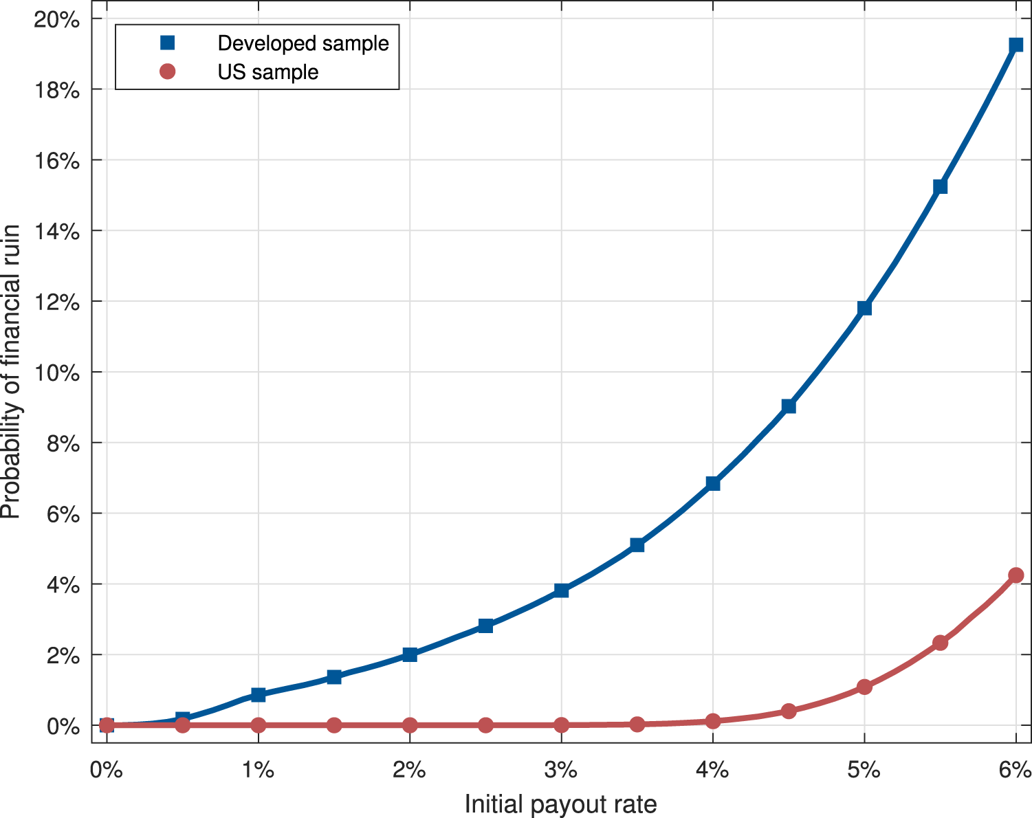
Analogous to our evaluation of the 4% rule, expected outcomes under these alternative withdrawal strategies are much worse with the developed market sample versus the US sample. For example, a guardrail strategy using an initial 4 percent rate faces a 6.8 percent likelihood of financial ruin based on the full sample compared with just a 0.1 percent likelihood with the US sample. The developed sample also implies greater risk of severe spending cuts resulting from poor financial market returns. In a similar vein, even though the constant percentage of wealth approach ensures that retirees never exhaust their savings (i.e., a couple only experiences financial ruin if their portfolio return is −100%), they face much greater risks over retirement consumption and ending wealth based on the developed market data. A couple withdrawing an annualized 4 percent of the portfolio balance has a 48 percent chance of an average real withdrawal amount that is less than the 4 percent initial payout level, compared with only a 29 percent likelihood using US data.Footnote 22 In short, regardless of the strategy under consideration, investors forming expectations from the small, biased US sample will be overly optimistic relative to those forming expectations from the broad sample of developed markets.
Our results for the 4% rule and the two alternative withdrawal rules highlight that popular retirement-spending heuristics are unlikely to offer resilient retirement consumption streams. None of the policies considered yields annual withdrawals that are simultaneously large relative to financial wealth at retirement, stable in real terms, and sufficiently likely to last through the retirement period. Our findings thus speak to the need to develop simple rules or investment vehicles for investors to build retirement savings and spend during retirement. Given the importance of longevity risk in the failures of withdrawal rules, annuity products that hedge against this risk could be targeted solutions to the problem. The SECURE 1.0 Act of 2019 and the SECURE 2.0 Act of 2022 broadened access to annuity products within retirement accounts, and qualified longevity annuity contracts (QLACs) that begin payments when the annuity buyer exceeds their actuarially expected lifespan could help bridge the gaps left after retirement savings are exhausted (e.g., Huang, Milevsky, and Young (Reference Huang, Milevsky Moshe and Young Virginia2017) and Horneff, Maurer, and Mitchell (Reference Horneff, Maurer and Mitchell Olivia2020, 2023)). But there is still work to be done to provide and expand access to actuarially fair QLACs that hedge longevity risk and support stable real consumption streams.
5.6. Alternative samples
Our main results for the safe withdrawal rate are based on historical asset-class performance over a long time series in a broad cross section of developed economies. Although this approach offers a wealth of new information relative to a US-centric design, it invites potential concerns that our findings are driven by historical periods that poorly reflect the expectations of today’s investors or by countries with smaller equity markets. We address these concerns by estimating the safe withdrawal rate for samples that exclude either the earlier data in our full sample or the countries with less-capitalized stock markets.
Panel D of Table 4 reports estimated withdrawal rates for ruin probabilities of 1 percent, 5 percent, and 10 percent for the developed country sample and the US sample using data only from the post-World War II period (October 1945 to December 2019). Panel E reports withdrawal rates for samples that condition on equity market size. To construct the sample for these simulations, we consider the full sample of developed countries, but we only include data for a given country after the year in which its market capitalization-to-GDP ratio first reaches 0.5.Footnote 23 The reported safe withdrawal rates in Panels D and E are similar to the corresponding estimates from our base case design. At a 5 percent ruin probability, for example, the developed country sample suggests a withdrawal rate of 2.70 percent for the post-World War II sample and a withdrawal rate of 2.65 percent for the sample conditioned on large equity market size. These estimates are just slightly higher than the base case withdrawal rate of 2.31 percent and considerably lower than the safe withdrawal rates implied by the US sample.
6. Discussion and conclusions
We study withdrawal rules for retirees, bringing to bear a wealth of information on the historical performance of major asset classes in developed countries. Our comprehensive new dataset mitigates the survivor and easy data biases that plague prior work. We find that there is no withdrawal rate that allows most retirees to maintain a reasonable standard of living while being virtually assured they will not outlive their wealth. Even if a couple is willing to bear a 5 percent ruin probability, the withdrawal rate is just 2.31 percent. This modest withdrawal rate implies that households must accumulate substantial savings to avoid severe spending cuts during retirement.
Beyond its advice for individuals, our study has implications for society and public policy. Retirees in a given cohort experience the same asset returns in retirement, such that financial ruin outcomes driven by poor investment performance are highly correlated. Under the prevailing 4% rule, our estimates suggest that generations of retirees jointly face great risk of financial ruin. Financial ruin for a cohort (or multiple consecutive cohorts) of retirees from an extended period of poor returns may lead to widespread poverty among the elderly and increased enrollment in means-tested social programs (e.g., Medicaid and Section 8 housing). As such, overestimating the safe withdrawal rate effectuates both individual and societal costs. When combined with the growing threat of Social Security’s insolvency (Board of Trustees, 2021) and the defined benefit pension’s demise, popular retirement spending rules place the three-legged stool of retirement (e.g., Poterba (Reference Poterba James2014)) in a precarious position. Our findings emphasize the need to develop and popularize simple, yet robust, tools to strengthen the role of savings in retirement, lest we awaken to find that the three-legged stool hasn’t a leg to stand on.
Acknowledgements
We thank Benjamin Felix, Ashish Tiwari, and Harry Turtle for helpful comments and suggestions. This research was supported by a grant from the Robert J. Trulaske, Sr. College of Business Large Grant Program.
Declarations of interest
None.
Appendix A. Supplementary appendix
In this appendix, we present additional empirical results.
A.1. Single retirees
Our main results in Section 5 correspond to joint investment-longevity outcomes for 65-year-old couples as a function of the real portfolio withdrawal rate, the retirement date, and the portfolio investment strategy. This appendix provides the corresponding results for single females and single males.
Table A.I presents distributional statistics for remaining life expectancy for 65-year-old females and 65-year-old males at various retirement dates. Table A.II shows safe real withdrawal rates for these investor types for various combinations of asset allocation strategy, retirement date, sample screens, tolerance for likelihood of financial ruin, and underlying data sample.
Distribution of time to death for single investors. The table summarizes the distribution of remaining life expectancy in years of a 65-year-old female (Panel A) and a 65-year-old male (Panel B) at various retirement dates. The distributions are constructed using the actuarial life tables from the Social Security Administration.

Withdrawal rates for single investors. The table shows the real payout rate in percentage estimated from 1,000,000 bootstrap simulations for various asset allocation strategies, retirement dates, and underlying data samples (i.e., the full sample of developed countries and the post-1925 US sample). The base case design (denoted with a  $\dagger$) corresponds to an asset allocation strategy of 60% stocks and 40% long-term bonds and a retirement date of 2022. The alternative cases modify the asset allocation strategy, the retirement date, or the data sample, as described in the table. For each design, the table reports withdrawal rates corresponding to 1%, 5%, and 10% probabilities of financial ruin. The investor type in Panel A (Panel B) is a 65-year-old female (65-year-old male).

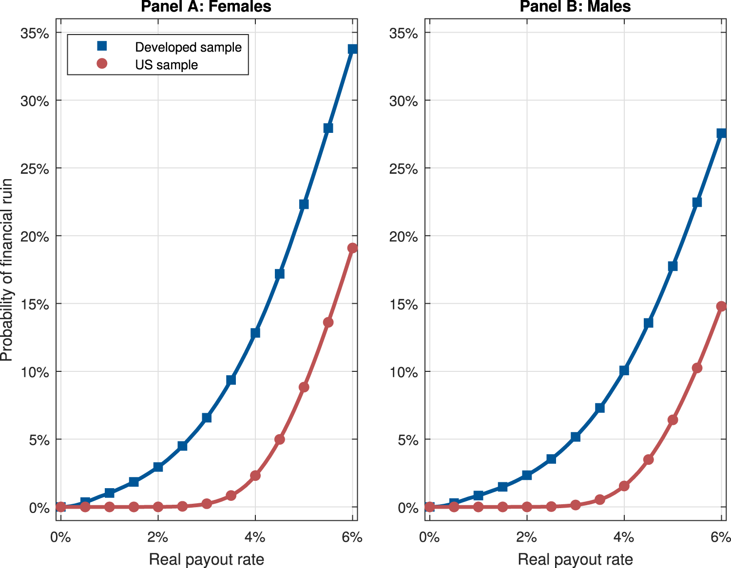
Figure A.1 shows the probability of financial ruin as a function of the real withdrawal rate for single females and males, and Figure A.2 summarizes the distribution of the bequest ratio for these investor types.
Probability of financial ruin for single investors. Panel A (Panel B) plots the likelihood that a 65-year-old female (65-year-old male) fully depletes retirement wealth prior to death as a function of the real withdrawal rate. The assumed asset allocation mix is 60% stocks and 40% bonds, and the survival probabilities are based on the 2022 actuarial life tables from the Social Security Administration. The blue (red) line shows the proportion of bootstrap simulations using the pooled sample of all developed countries (post-1925 US sample) in which wealth reaches zero prior to death. We simulate 1,000,000 joint portfolio return and survival outcomes for each combination of sample and withdrawal rate.

Distribution of bequest ratio for single investors. Panel A (Panel B) plots the distribution of the ratio of real ending wealth to real wealth at the start of retirement for a 65-year-old female (65-year-old male) as a function of the real withdrawal rate. Real ending wealth is the real wealth at the time of death. The assumed asset allocation mix is 60% stocks and 40% bonds, and the survival probabilities are based on the 2022 actuarial life tables from the Social Security Administration. The blue (red) plot corresponds to the distribution of the bequest ratio across bootstrap simulations using the pooled sample of all developed countries (post-1925 US sample). The solid lines indicate the median bequest ratios, and the shaded regions covers the 10th–90th percentiles of the distributions. We simulate 1,000,000 joint portfolio return and survival outcomes for each combination of sample and withdrawal rate.

A.2. Alternative stock-bond allocations
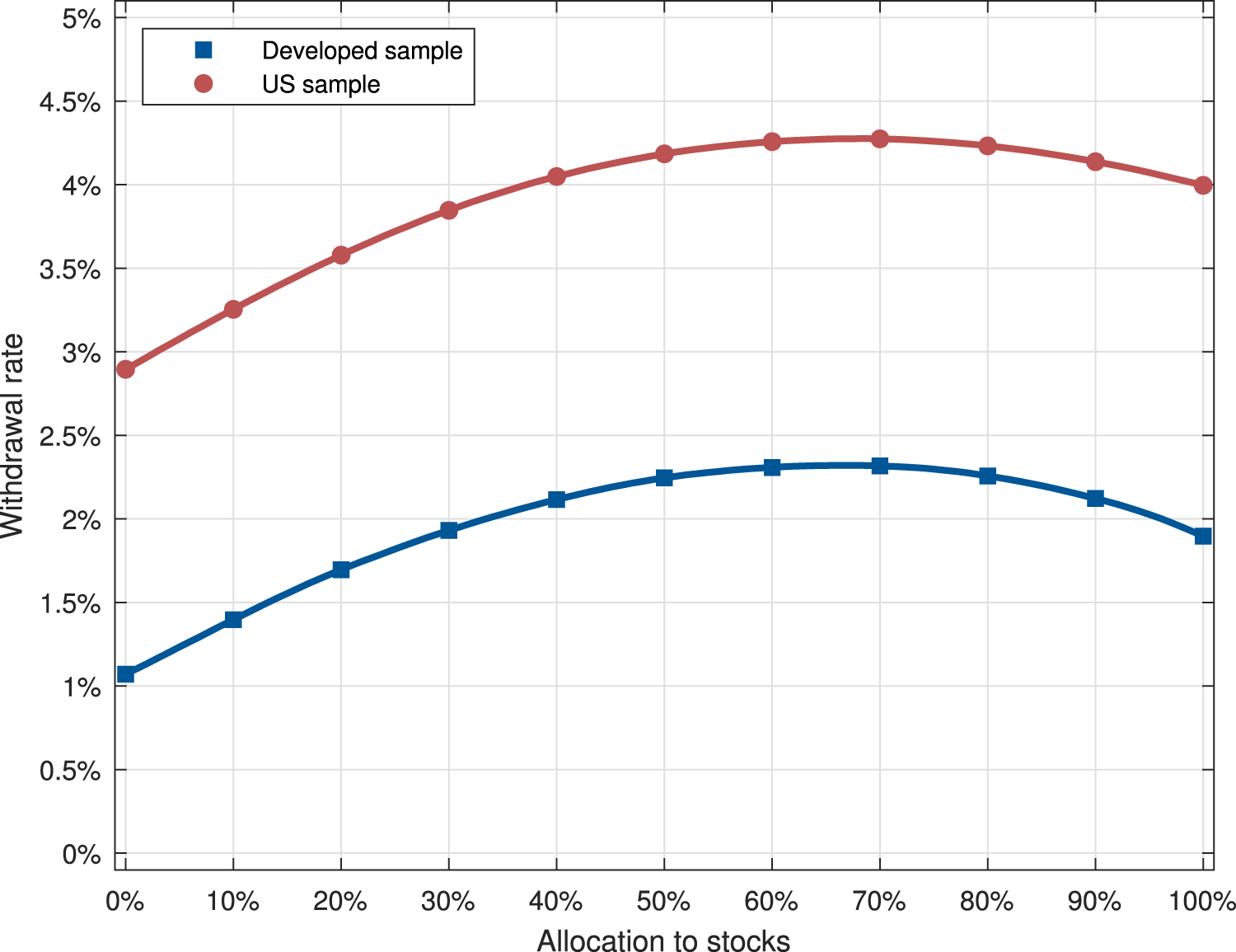
In Table 4, we report safe withdrawal rates for several static portfolio strategies that allocate across stocks and bonds. These strategies have allocations to stocks that range from 0 percent to 100 percent in increments of 20 percent. For completeness, Figure A.3 plots the safe withdrawal rate corresponding to a 5 percent probability of financial ruin for all long-only stock-bond strategies. For the developed sample (US sample), the maximum withdrawal rate of 2.32% (4.28%) corresponds to a stock allocation of 68% (69%).
Withdrawal rates for alternative stock-bond allocations. The figure plots the real payout rate in percentage estimated from 1,000,000 bootstrap simulations for strategies adopting static allocations to domestic stocks and domestic bonds. The blue (red) line shows the withdrawal rate estimated from the pooled sample of all developed countries (post-1925 US sample). For each design, the withdrawal rate corresponds to a 5% probability of financial ruin.

A.3. Alternative withdrawal policies
We focus in Section 5 on rules that specify a constant real withdrawal amount because of the ubiquity of the 4% rule. This appendix considers two alternative withdrawal strategy designs:
(1) Guardrails approach: Given initial wealth W 0 and adopted withdrawal rule r, the couple withdraws
$I_0=\frac{W_0r}{12}$ at the beginning of each month in the first year. In subsequent years, the real monthly withdrawal amount It potentially increases or decreases depending on portfolio performance following the strategy outlined by Klinger (Reference Klinger William2016). Monthly real retirement wealth evolves as
(A1)\begin{equation}
W_{t+1}=\max(W_t - I_t,0)R_{p,t+1}.
\end{equation}At the beginning of each year from the second year of retirement through the 15th year, with the first month of the given year indexed as t, the couple evaluates whether the previous withdrawal amount
$I_{t-1}$ remains appropriate given their current wealth level Wt. If
$I_{t-1} \gt 1.2\times \frac{W_tr}{12}$ (i.e., the status quo withdrawal amount is more than 20% higher than a withdrawal amount calculated from current wealth and the adopted withdrawal rule), then
$I_t=0.9\times I_{t-1}$ (i.e., the withdrawal rate is reduced by 10%). Symmetrically, the withdrawal amount increases by 10 percent if current wealth is sufficiently high, i.e., if
$I_{t-1} \lt 0.8\times \frac{W_tr}{12}$ then
$I_t=1.1\times I_{t-1}$. The couple then maintains constant real withdrawal amounts until death. An exception to this evolution of withdrawal amounts occurs in cases with very low financial wealth or financial ruin (i.e.,
$W_t \lt I_t$ or
$W_t=0$), as the actual payout is equal to
$\min(I_t,W_t)$ in each month.(2) Constant proportion of wealth approach: Given initial wealth W 0 and adopted withdrawal rule r, the couple withdraws
$I_0=\frac{W_0r}{12}$ in the first month. In all subsequent months, the couple withdraws
$I_t=\frac{W_tr}{12}$. Monthly real retirement wealth evolves as
(A2)\begin{equation}
W_{t+1}=\max(W_t - I_t,0)R_{p,t+1}.
\end{equation}Financial ruin only occurs if the gross portfolio return
$R_{p,t+1}$ equals zero (i.e., the net portfolio return is −100% in a given month). Given our sample of data and portfolio strategies that do not take levered or short positions, the gross portfolio return is always positive such that financial ruin occurs with zero probability.


Figures A.4–A.6 show results for the guardrails strategy with initial withdrawal rates ranging from 0 percent to 6 percent. Each figure summarizes retirement outcomes using the developed country sample (blue) and the US sample (red). Figure A.4 plots the probability of financial ruin as a function of the initial real withdrawal rate, and Figure A.5 summarizes the distribution of the bequest ratio. Given that the guardrails strategy makes adjustments to monthly real withdrawal amounts based on portfolio performance, the average real withdrawal rate as a percentage of initial wealth at retirement could be lower or higher than the initial withdrawal rate. Figure A.6 summarizes the distribution of the average real withdrawal rate.
Probability of financial ruin for guardrails strategy. The figure plots the likelihood that a 65-year-old couple fully depletes their retirement wealth prior to the death of the last survivor as a function of the initial withdrawal rate under the guardrails strategy. The assumed asset allocation mix is 60% stocks and 40% bonds, and the survival probabilities are based on the 2022 actuarial life tables from the Social Security Administration. The blue (red) line shows the proportion of bootstrap simulations using the pooled sample of all developed countries (post-1925 US sample) in which wealth reaches zero prior to the death of the last survivor. We simulate 1,000,000 joint portfolio return and household survival outcomes for each combination of sample and withdrawal rate.

Distribution of bequest ratio for guardrails strategy. The figure plots the distribution of the ratio of real ending wealth to real wealth at the start of retirement for a 65-year-old couple as a function of the initial withdrawal rate under the guardrails strategy. Real ending wealth is the real wealth at the time of death of the last survivor. The assumed asset allocation mix is 60% stocks and 40% bonds, and the survival probabilities are based on the 2022 actuarial life tables from the Social Security Administration. The blue (red) plot corresponds to the distribution of the bequest ratio across bootstrap simulations using the pooled sample of all developed countries (post-1925 US sample). The solid lines indicate the median bequest ratios, and the shaded regions covers the 10th–90th percentiles of the distributions. We simulate 1,000,000 joint portfolio return and household survival outcomes for each combination of sample and withdrawal rate.

Distribution of average real withdrawal rate for guardrails strategy. The figure plots the distribution of the average real withdrawal rate (as a proportion of wealth at the start of retirement) during retirement for a 65-year-old couple as a function of the initial withdrawal rate under the guardrails strategy. The assumed asset allocation mix is 60% stocks and 40% bonds, and the survival probabilities are based on the 2022 actuarial life tables from the Social Security Administration. The blue (red) plot corresponds to the distribution of the average real withdrawal rate across bootstrap simulations using the pooled sample of all developed countries (post-1925 US sample). The solid lines indicate the median average real withdrawal rates, and the shaded regions covers the 10th–90th percentiles of the distributions. We simulate 1,000,000 joint portfolio return and household survival outcomes for each combination of sample and withdrawal rate.

Figures A.7 and A.8 present results for the constant proportion of wealth strategy. The financial ruin probability is 0 percent for this strategy, so we summarize the distributions of bequest wealth (Figure A.7) and the average real withdrawal rate as a percentage of initial wealth at retirement (Figure A.8).
Distribution of bequest ratio for constant proportion of wealth strategy. The figure plots the distribution of the ratio of real ending wealth to real wealth at the start of retirement for a 65-year-old couple as a function of the withdrawal rate under the constant proportion of wealth strategy. Real ending wealth is the real wealth at the time of death of the last survivor. The assumed asset allocation mix is 60% stocks and 40% bonds, and the survival probabilities are based on the 2022 actuarial life tables from the Social Security Administration. The blue (red) plot corresponds to the distribution of the bequest ratio across bootstrap simulations using the pooled sample of all developed countries (post-1925 US sample). The solid lines indicate the median bequest ratios, and the shaded regions covers the 10th–90th percentiles of the distributions. We simulate 1,000,000 joint portfolio return and household survival outcomes for each combination of sample and withdrawal rate.

Distribution of average real withdrawal rate for constant proportion of wealth strategy. The figure plots the distribution of the average real withdrawal rate (as a proportion of wealth at the start of retirement) during retirement for a 65-year-old couple as a function of the withdrawal rate under the constant proportion of wealth strategy. The assumed asset allocation mix is 60% stocks and 40% bonds, and the survival probabilities are based on the 2022 actuarial life tables from the Social Security Administration. The blue (red) plot corresponds to the distribution of the average real withdrawal rate across bootstrap simulations using the pooled sample of all developed countries (post-1925 US sample). The solid lines indicate the median average real withdrawal rates, and the shaded regions covers the 10th–90th percentiles of the distributions. We simulate 1,000,000 joint portfolio return and household survival outcomes for each combination of sample and withdrawal rate.

A.4. Alternative sample conditioned on equity market size
In Section 5.6 of the paper, we estimate safe withdrawal rates for a sample of developed countries that only includes data for a given country after the year in which its market capitalization-to-GDP ratio first reaches 0.5. Table A.III reports the sample start date for each developed country in this alternative sample.
Country eligibility dates for sample conditioned on large equity market size. The table shows the sample start dates for developed countries in the alternative sample using a screen for equity market size. The sample formation process is described in Section 5.6.