2.1.1. Parametrisation of the base flow

As can be seen in figure 2, the mean flow profiles downstream of the first Mach disk are, as expected, composed of two mixing layers: one separating the supersonic flow and the ambient one, the other one separating the subsonic core and the supersonic flow. A representative analytical formulation of this base flow is obtained by connecting three uniform regions, the inner, the annular and the external one, with two hyperbolic tangent profiles to account for the mixing layers:

(2.1) \begin{eqnarray} q_{in}(r) & = & q_{i}\left[1 - \left (1-\frac {q_a}{q_i}\right )\left (1+\tanh \left (\frac {2}{\theta _{i}}(r-R_i)\right )\right ) \right] \nonumber \\q_{out}(r) & = & 1 - \frac {1}{2}\left (1-\frac {q_e}{q_a}\right )\left (1+\tanh \left (\frac {2}{\theta _{e}}(r-R_e)\right )\right ) \nonumber \\ q(r) & = & {q_{in}(r)} \cdot {q_{out}(r)}, \end{eqnarray}

where $q$ here stands for $M$ , $\bar {\rho }$ or $\bar {T}$ . The indices i, a, and e respectively refer to the inner, the annular and the external flow variable of interest. The values $(R_{i}, \theta _{i})$ , $(R_{e}, \theta _{e})$ are the inner and external mixing layer radial positions and thicknesses, respectively. A regression of the analytical profiles onto numerical data available (numerical simulation previously done in Bakulu et al. (Reference Bakulu, Lehnasch, Jaunet, Goncalves da Silva and Girard2021)) gives access to the parameters. The reader should note that different mixing layer positions and thicknesses may be attributed to the mean velocity, density or temperature profile when a direct fit to the numerical data are performed. As far as the flow velocity profile is concerned, this formulation is equivalent to the one used in Michalke (Reference Michalke1984). This modelisation differs from that chosen by Bhat & Seiner (Reference Bhat and Seiner1993), who preferred Gaussian profiles instead of hyperbolic tangent ones.

Optimal analytical profiles are compared with the reference numerical data in figure 2, demonstrating the ability of the analytical functions chosen to represent the computed flow field. The reader may note that the velocity and temperature profiles are not constant in the supersonic stream. This cannot be accounted for using the chosen analytical formulation and the modelled profiles show a plateau in this region. It is believed that this simplification will not lead to a drastic change in the results, as the velocity and temperature variation within the supersonic stream are very small compared with the variations in the mixing layers.

Figure 2.

Typical base flow used for the study of local stability properties of the flow. The considered profiles are extracted at the distance from the throat $x/D = 1.6$ (where $D$ is the exit nozzle diameter), in between the two first Mach disks of the flow. Dots represent the numerical data and red lines are the fitted analytical functions.

2.1.2. Obtaining the base flow parameters

Annular supersonic flows are commonly encountered when flows exit convergent–divergent nozzles and often exhibit a sufficiently large Mach disk within their core (Hadjadj & Onofri Reference Hadjadj and Onofri2009). A simplified analytical description of the shock wave network is proposed in various studies using mass and momentum conservation, for example, in Chow & Chang (Reference Chow and Chang1975) and Li & Ben-Dor (Reference Li and Ben-Dor1998). We opted to derive an even simpler description of the flow, using quasi-one-dimensional relations, to obtain the parameters that our finite thickness model requires. Indeed, the earlier-presented base flows can be parameterised with the following set of parameters: ( $r_i, r_e, M_i, M_e, M_a, T_i, T_a$ ). In this section, we often use commas to indicate interchangeable indices for conciseness. 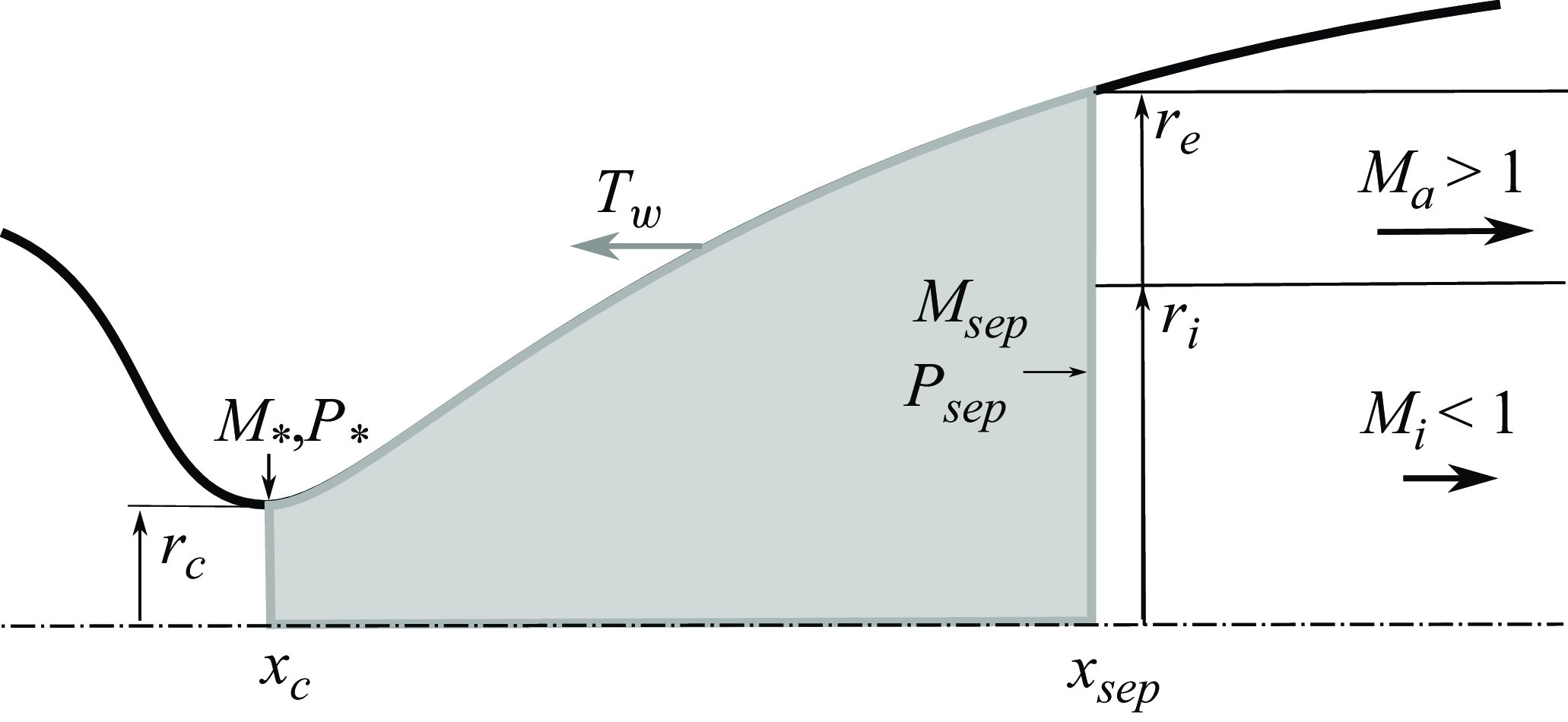For example, the former vector of parameters could be written as ( $r_{i,e}, M_{i,e,a}, T_{i,a}$ ) with this notation. Basic fluid mechanics principles reveal that these parameters are interconnected and we cannot assume arbitrary values. Hence, to attain a meaningful parameter set, a simplified model of the flow inside the nozzle is built, assuming quasi-one-dimensional behaviour from the throat to the separation point, where the annular supersonic flow is presumed to originate. The simplified flow configuration and the associated control volume that we use for that purpose are illustrated in figure 3.

Figure 3.

Schematic of the control volume employed to parameterise the flow field.

By applying mass conservation to the control volume bounded by the nozzle throat and the attached flow (as depicted in grey in figure 3), we derive the equation

(2.2) \begin{eqnarray} \rho _* U_* D_c^2 &=& \rho _i U_i D_i^2 + \rho _a U_a (1-D_i^2), \end{eqnarray}

where $(\cdot )_*$ denotes sonic variables at the throat and $D_{i,c} = {D_{i,c}}/{D_e}$ represents the normalised radius of the inner ( $\cdot _i$ ) vortex sheet or the throat ( $\cdot _c$ ) relative to the external vortex sheet.

Noting that $\mathcal {M}$ , the local Mach number, differs from the acoustic Mach number employed in the subsequent linearised dynamical model, $\mathcal {M} = M \cdot {c_\infty }/{c}$ , where $c$ is the local speed of sound, the following relation can be easily obtained from the previous equation:

(2.3) \begin{eqnarray} {\left (1+\frac {\gamma -1}{2}\right )^{-\frac {\gamma +1}{2(\gamma -1)}}} \frac {P_{t0}}{\sqrt {T_{t0}}} D_c^2 &=& \frac {P_i}{\sqrt {T_i}} \mathcal {M}_i D_i^2 + \frac {P_a}{\sqrt {T_a}} \mathcal {M}_a (1-D_i^2), \end{eqnarray}

where $P_{t0}$ and $T_{t0}$ , respectively, are the total pressure and temperature of the flow, and $P_{i,a}$ and $T_{i,a}$ , respectively, are the static pressure and temperature of the inner ( $\cdot _,i$ ) and annular ( $\cdot {,a}$ ) streams. Assuming an isobaric jet for simplification, i.e. $P_a = P_i = P_\infty$ , the mass conservation equation can be further simplified to (see Appendix A for further details)

(2.4) \begin{eqnarray} \beta _m {D_c^2} &=& (\mu _i - \mu _a) {D_i^2} + \mu _a, \end{eqnarray}

where

(2.5) \begin{align} \mu _{i,a} =& { \mathcal {M}_{i,a} \sqrt {1+\frac {\gamma -1}{2}\mathcal {M}_{i,a}^2}} \end{align}

(2.6) \begin{align} \beta _m =& {\left (1+\frac {\gamma -1}{2}\right )^{-\frac {\gamma +1}{2(\gamma -1)}}} \frac {P_{t0}}{P_\infty }. \end{align}

In essence, the mass conservation equation establishes a connection between the nozzle pressure ratio $NPR = {P_{t0}}/{P_\infty }$ , its geometry and the Mach numbers of both the annular and internal jets. The NPR is dictated by the nozzle’s operational regime, and $D_c$ is given by nozzle design considerations.

Considering momentum conservation along the axial direction within the same control volume, while neglecting body and viscous forces, leads to the equation

(2.7) \begin{eqnarray} {\beta _q} D_c^2 - \frac {F_w}{P_\infty } & = & \gamma D_i^2 \left ( \mathcal {M}_i^2 - \mathcal {M}_a^2 \right ) + \left (\gamma \mathcal {M}_a^2 + 1\right ), \end{eqnarray}

where

(2.8) \begin{equation} \beta _q = (1+\gamma )\left (1+\frac {\gamma -1}{2}\right )^{\frac {-\gamma }{\gamma -1}} \frac {P_{t0}}{P_\infty }, \end{equation}

and $F_w$ represents the pressure forces acting on the nozzle wall. It is important to note that $F_w$ depends on the nozzle geometry and can be approximated using characteristic methods. By solving this equation, we derive an analytical expression for $D_i^2$ given by

(2.9) \begin{eqnarray} D_i^2 &=&\frac {1}{\gamma \left (\mathcal {M}_i^2 - \mathcal {M}_a^2\right )}\left [ {\beta _q} D_c^2 - \frac {F_w}{P_\infty } - \left ( \gamma \mathcal {M}_a^2 +1 \right )\right ], \end{eqnarray}

which can subsequently be substituted into the mass conservation equation. This substitution leads to an equation for the annular Mach number, providing that $\mathcal {M}_{i}$ and $F_w$ are known:

(2.10) \begin{eqnarray} {\frac {\mu _i - \mu _a}{\gamma \left (\mathcal {M}_i^2 - \mathcal {M}_a^2\right )} \left [ {\beta _q}{D_c^2} - \frac {F_w}{P_\infty } - \left ( \gamma \mathcal {M}_a^2 + 1 \right )\right ] } + \mu _a - \beta _m &=& 0, \end{eqnarray}

where

(2.11) \begin{align} \mu _{i,a} =& { \mathcal {M}_{i,a} \sqrt {1+\frac {\gamma -1}{2}\mathcal {M}_{i,a}^2}} \end{align}

(2.12) \begin{align} \beta _m =& {\left (1+\frac {\gamma -1}{2}\right )^{-\frac {\gamma +1}{2(\gamma -1)}}} \frac {P_{t0}}{P_\infty } \end{align}

(2.13) \begin{align} \beta _q =& (1+\gamma )\left (1+\frac {\gamma -1}{2}\right )^{\frac {-\gamma }{\gamma -1}} \frac {P_{t0}}{P_\infty }. \end{align}

It is worth mentioning that, once $M_{i,a}$ are known, $T_{i,a}$ can be determined via the usual isentropic relations, using the typically known total temperature of the flow.

2.1.3. Solving the base flow model

Equation (2.10) can be solved to determine the Mach number of the annular flow, adhering to the fundamental principles of fluid mechanics. This can be achieved for any given input parameter set containing the nozzle pressure ratio $NPR = {P_{t0}}/{P_\infty }$ , throat diameter $D_c$ , inner subsonic Mach number $\mathcal {M}_i$ and nozzle thrust $F_w$ . These parameters are intrinsically interconnected and must be chosen judiciously. In what follows, we elucidate how these parameters can be defined based on the nozzle’s pressure and Mach number profiles, along with the application of a classical separation criterion. We assume that flow separation occurs at an axial location within the nozzle, denoted by $x_{sep}$ , where an isentropic expansion of the flow inside the nozzle has resulted in a local Mach number $\mathcal {M}_{sep}$ and pressure $P_{sep}$ .

First, it is evident from figure 3 that our reference length scale, $D_e$ , can be equated to the diameter of the nozzle at the separation point $D_w$ :

(2.14) \begin{equation} D_e = D_w(x_{sep}). \end{equation}

This implies that the reference length scale for the annular jet flow will vary according to the NPR.

Second, experimental observations suggest that the separation pressure $P_{sep}$ is related to the separation Mach number and the external pressure $P_{\infty }$ through a suitably chosen separation criterion:

(2.15) \begin{equation} \frac {P_{sep}}{P_\infty } = F(\mathcal {M}_{sep}), \end{equation}

where $F$ represents the separation criterion formula, which enables the determination of $P_{sep}$ . Subsequently, assuming an isentropic expansion from the tank to the separation point, the NPR at the current flow condition can be calculated as

(2.16) \begin{equation} \frac {P_{t0}}{P_\infty } = {F(\mathcal {M}_{sep})}{\left (1+\frac {\gamma -1}{2} \mathcal {M}_{sep}\right )^{\frac {\gamma }{\gamma -1}}}. \end{equation}

An approximation for the inner Mach number $\mathcal {M}_i$ can be derived by considering that the Mach disk is formed at the upstream Mach number $\mathcal {M}_{sep}$ :

(2.17) \begin{equation} \mathcal {M}_i = \frac {(\gamma -1)\mathcal {M}_{sep}^2+2}{2\gamma \mathcal {M}_{sep}^2-(\gamma -1)}. \end{equation}

It is important to note that this approximation leads to an overestimation of $\mathcal {M}_i$ since, in real flow conditions, the Mach disk always forms downstream of the separation point, and hence at higher Mach numbers.

Finally, the thrust of the control volume, $F_w$ , can be determined by integrating the wall pressure along the nozzle from the throat to the separation point $x_{sep}$ :

(2.18) \begin{equation} F_w = \int _{x_c}^{x_{sep}} \left (P_\infty - P_w \right ) (\boldsymbol {n} \cdot \boldsymbol {i} \,) \; {\rm d}S. \end{equation}

The model is now complete and only requires the nozzle wall radius and Mach number profiles, which can be computed using methods such as the method of characteristics. An example using nozzle characteristics from Jaunet et al. (Reference Jaunet, Arbos, Lehnasch and Girard2017) is presented in the following section. The acoustic Mach numbers of the vortex sheets and the inner radius satisfying the proposed model are depicted in figure 4 against the fully expanded Mach number of the flow $M_j$ . The value of $M_j$ can be computed easily from the nozzle NPR using isentropic relations. The separation criterion from Stark (Reference Stark2005), with slight modifications to better align with the experimental observations of Jaunet et al. (Reference Jaunet, Arbos, Lehnasch and Girard2017) for this nozzle geometry, is employed. The decrease in $\mathcal {M}_i$ as the normal shock wave strengthens with downstream displacement of the separation, is in accordance with expectations. Conversely, neither $M_a$ nor $D_i$ display a monotonic behaviour. This can be attributed to the nozzle wall profile approaching a near-horizontal orientation near the lip, resulting in saturation of thrust $F_w$ . Another noteworthy behaviour is the sudden decrease in $D_i$ as the separation approaches the nozzle lip, which is consistent with the behaviour of overexpanded jets from TIC nozzles – akin to an approaching adaptation where the Mach disk diminishes or disappears.

Mach number and inner shear layer location values obtained for $M_j = 2.09$ are indicated as diamonds in figure 4. Table 1 compares the predictions of the model with those observed in numerical simulations from Bakulu et al. (Reference Bakulu, Lehnasch, Jaunet, Goncalves da Silva and Girard2021), specifically after the first Mach disk. The results are summarised in table 1. As seen, the proposed model accurately predicts Mach numbers within a $\pm$ 10 % range but tends to overestimate $D_i$ . This discrepancy is due to assuming a horizontal flow exit from separation, which is erroneous as the flow is deflected through the separation shock wave. However, this representation acknowledges its simplified nature. Adjusting the empirical separation model, or using a more representative value for $D_e$ , would yield slightly different values for $M_{i,a}$ and $D_i$ . Despite these uncertainties, it is believed that the model remains valuable for understanding the overall dynamics of the flow.

Figure 4.

Variation of Mach numbers (a) and location of inner vortex sheet diameters (b) with the fully expanded jet Mach number.

Table 1.

Comparison of Mach numbers and inner shear layer locations obtained from the DDES of Bakulu et al. (Reference Bakulu, Lehnasch, Jaunet, Goncalves da Silva and Girard2021) and the proposed simplified model.

In conclusion, we have formulated a comprehensive model that derives essential parameters for feeding a simplified linear dynamical model of jet flows exiting from over-expanded nozzles. This model requires the a priori knowledge of the static pressure and Mach number profiles along the nozzle, and a separation criterion. From this, all the necessary quantities to build a simplified mean annular supersonic mean flow for various nozzle regimes can be retrieved.

3.1.1. K–H mode

In figure 8, we plot the growth rate evolution of both K–H modes as a function of $R_i$ for various Strouhal numbers. The outer K–H mode is always more unstable than the inner one for all the configurations investigated in this study. This is expected considering that the velocity gradient is stronger for the outer mixing layer than for the inner one. The outer mode becomes even more unstable as $R_i$ increases, although at high frequencies its growth rate shows a plateau at low values of $R_i$ . On the other hand, the inner mixing layer instability shows an optimal growth rate at specific $R_i$ values. This trend suggests that there may exist specific base flows and frequencies for which the inner and outer K–H modes possess equivalent growth rates. In some cases, the inner mode can become even more unstable than the outer one. However, this is more likely to occur at higher frequencies and might not be relevant for the initial nozzle flow problem, where resonance at lower frequencies is observed.

Figure 8.

Growth rate of the K–H mode as a function of the Strouhal number and the inner mixing layer location $R_i$ . Dashed lines and solid lines correspond to the inner and outer K–H modes, respectively.

The pressure eigenfunctions associated with the two identified K–H modes are presented in figure 9 for $St=0.2$ . As expected, the eigenfunction is maximum at the mixing layer location and is zero at the centre line, as we focus on the $m=1$ anti-symmetric wavenumber. The outer K–H mode does not seem to be significantly affected by the inner mixing layer, unlike the inner mode whose support spreads further to the outside the outer mixing layer as the two mixing layers get closer. Interestingly, the radial support of the inner K–H wave decays less rapidly than that of the outer one. This allows the inner mode to be detected quite far from the jet and enables it to exchange energy with feedback waves outside the supersonic annular region. This aligns well with the observations of Bakulu et al. (Reference Bakulu, Lehnasch, Jaunet, Goncalves da Silva and Girard2021), who found that the inner mixing layer supports most of the perturbations associated with the resonance process in their flow.

Figure 9.

Eigenfunctions associated with the inner (dashed) and outer (solid) K–H modes, normalised with respect to their maximum values, for $St=0.2$ and $St=0.4$ .

3.1.2. GJM

GJM have been shown to play a significant role in the resonance of screeching and impinging jets (see, for example, Gojon et al. (Reference Gojon, Bogey and Mihaescu2018); Jaunet et al. (Reference Jaunet, Mancinelli, Jordan, Towne, Edgington-Mitchell, Lehnasch and Girard2019); Mancinelli et al. (Reference Mancinelli, Jaunet, Jordan and Towne2021); Edgington-Mitchell et al. (Reference Edgington-Mitchell, Jaunet, Jordan, Towne, Soria and Honnery2018)). Their dispersion relation is a key characteristic that explains cut-on and cut-off frequencies, and the transition from axisymmetric to helical modes, and it improves the model predictions (Mancinelli et al. Reference Mancinelli, Jaunet, Jordan and Towne2019; Nogueira et al. Reference Nogueira, Jordan, Jaunet, Cavalieri, Towne and Edgington-Mitchell2022). As explained previously, their eigenvalues lie on the real axis of the spectrum until they become evanescent. Figure 7 shows that the annular jet configuration, as encountered in the exhaust of over-expanded Convergent-Divergent (CD) nozzles, also supports such types of waves. In the $(k_r,St)$ plane, this occurs at the summit of a given branch. At supersonic speeds, jets support both upstream propagation, denoted by $k_p^-$ , and downstream propagation, denoted by $k_p^+$ , GJM. This distinction is made based on the sign of their group velocity $u_g = {\partial \omega }/{\partial k}$ , and hence corresponds to the local slope of their dispersion relation presented in figure 10. The $k_p^-$ can be seen close to the acoustic waves dispersion relation and is the mode that can carry energy in the upstream direction. The dispersion relation of these waves is plotted in figure 10 in the $St{-}k_r$ plane for various positions of the inner mixing layer.

Figure 10.

Neutral mode dispersion relation for various positions of the inner mixing layer: $R_i = 0.05$ (a), $R_i = 0.1$ (b), $R_i = 0.2$ (c) and $R_i = 0.30$ (d). The dash-dotted line corresponds to the acoustic wave dispersion relation.

As expected, at each $R_i$ , the neutral waves form families of modes hierarchically ordered by their radial supports: higher frequencies correspond to higher radial orders (i.e. the number of nodes and antinodes; see Tam & Hu (Reference Tam and Hu1989)). As seen, the position of the inner mixing layer has a strong impact on the dispersion relation of the neutral modes: as $R_i$ increases, the frequencies at which the modes are encountered also increase. Furthermore, the group velocity of the $k_p^+$ mode decreases with increasing $R_i$ . This can be understood by recognising that, for $R_i=0$ or $R_i=R_e$ , the base flow is close to a supersonic top-hat jet or a subsonic one, respectively. As can be seen, both group and phase velocities of the guided jet modes decrease with increasing $R_i$ . This is expected from the decrease of the overall average speed of the jet when $R_i$ increases. The behaviour of the neutral modes seems to lie between what is expected for a subsonic $M=M_i\lt 1.0$ jet and a supersonic $M=M_a\gt 1.0$ one.

Moreover, we observe that $R_i$ affects the domain of existence of the upstream propagating neutral modes, which are the modes in the dispersion relation with negative group velocity. First, the domain where $d\omega /dk\lt 0$ shifts towards higher Strouhal numbers with increasing $R_i$ . Second, the range of Strouhal numbers where these neutral modes are encountered varies significantly with $R_i$ : larger $R_i$ providing a wider range of existence, and therefore offering more solutions for possible resonances.

The eigenfunctions associated with the upstream propagating neutral modes are presented in figure 11 for $St=0.1$ and $St=0.2$ . As expected, the radial supports of these modes share common features with Bessel functions. At low Strouhal numbers, the eigenfunctions show one antinode, while for higher frequencies, more antinodes can be observed. Surprisingly, very little change in the radial support is observed for varying $R_i$ . This is due to the fact that these modes are duct-like modes, so that their support is mostly independent of the base flow, in contrast to their wavenumber. It is important to notice that they also have support outside the jet, similar to the inner K–H wave. This allows these waves to interact and for the upstream mode to carry energy upstream, potentially closing a feedback loop.

Figure 11.

Eigenfunctions associated with the guided jet modes, normalised with respect to their maximum values, for $St=0.1$ and $St=0.2$ .

3.2.1. K–H mode

Figure 13 shows the growth rate of both K–H modes with varying thicknesses and Strouhal numbers. As expected, larger mixing layer thicknesses result in lower growth rates of the K–H mode. For the base flows and frequencies considered here, the inner mixing layer is more stable than the outer one. This is due to their difference in velocity gradient. The outer mixing layer separates a supersonic stream from a quiescent atmosphere, while the inner one separates two rapid flows. Interestingly, for relatively high frequencies (greater than $St=0.2$ ), increasing the thickness stabilises the outer mixing layer more quickly than the inner one. Thus, there might be flow configurations for which both K–H modes exhibit comparable growth rates. Depending on the frequency and base flow, the dynamics may not be entirely dominated by the outer K–H mode, as one might initially assume.

Figure 13.

Growth rates of both the inner () and outer () K–H modes as functions of the mixing layer thicknesses and the Strouhal number.

The associated spatial profiles of the aforementioned K–H modes are presented in figure 14 for different Strouhal numbers and varying mixing layer thicknesses. We observe similar results to the previous study: for the thinnest mixing layer, the inner and outer K–H modes exhibit maximum pressure fluctuations at the locations where the base flow exhibits the maximum levels of velocity gradients. For all frequencies, thickening the mixing layer tends to spread the spatial support of the inner modes towards the outer mixing layer by increasing the pressure amplitude near the jet boundary. At the highest frequencies studied here, the signature of the outer K–H modes also spreads onto the inner mixing layer. As indicated earlier by their relative growth rates, the entanglement of spatial support of the K–H modes with increasing mixing layer thickness might make it difficult to distinguish their relative signatures in the fluctuating pressure field. Nonetheless, as mentioned in the previous section, the inner mixing layer K–H mode appears to have a slower radial decay compared with the outer one. This supports the findings of Bakulu et al. (Reference Bakulu, Lehnasch, Jaunet, Goncalves da Silva and Girard2021), which show that, at the resonance frequency, the downstream energy-carrying mode was supported by the inner mixing layer. The wide radial extent of the eigenfunction, as shown here, also suggests that the inner K–H mode can exchange energy with GJM or acoustic modes, whose support can be located outside the jet.

Figure 14.

Eigenfunctions associated with the inner (dashed) and outer (plain) K–H modes, normalised with respect to their maximum values, for $St=0.1$ (a), $St=0.2$ (b), $St=0.3$ (c) and $St=0.4$ (d).

3.2.2. GJM

The dispersion relation of the GJM for varying mixing layer thicknesses is now presented in figure 15. Unlike the dispersion relation of K–H modes, the dispersion relation of the GJM is only slightly affected by thicknesses of the mixing layers. There is a slight variation in the domain of existence of the upstream-travelling modes between the branch and saddle points, as pointed out by Towne et al. (Reference Towne, Cavalieri, Jordan, Colonius, Schmidt, Jaunet and Brès2017). The primary effect of thickening the mixing layers is on the group velocity ( $\partial \omega /\partial k$ ), with thicker mixing layers leading to lower group velocities, as one would expect.

Figure 15.

GJM dispersion relationship for varying mixing layer thicknesses.

Figure 16 presents the eigenfunctions of the computed GJM. Frequencies were selected so that modes of the same radial order appear on the same figure. Note that eigenfunctions obtained at the same frequency are plotted with the same line style. All computed eigenfunctions almost collapse onto the same line, indicating that the spatial support of the GJM is not affected by the thickening of the jet. The GJM are very robust and can still be observed even if the jet is strongly affected by the diffusion of momentum across the stream interfaces.

Figure 16.

GJM spatial support for the first radial order (a) and the second radial order (b). Colors indicate the mixing layer vorticity thickness, and different line styles are attributed to eigenfunctions of different frequencies.

3.3.1. K–H modes

The dynamical characteristics of the unstable K–H waves with respect to the base flows presented in the former paragraph are plotted in figure 18 for various frequencies. As expected from the previous results, both K–H waves are unstable, the outer one being the most unstable for all flow regimes and frequencies considered. The evolution of the growth rate of the inner K–H wave seems rather independent of the jet Mach number until $M_j = 2.0$ . For values greater than this expansion ratio, it is interesting to notice that the inner K–H wave is more and more unstable at all the frequencies considered. It is worth noting that this value is very close to the value of $M_j=2.09$ around which resonances have been experimentally observed (Jaunet et al. Reference Jaunet, Arbos, Lehnasch and Girard2017). The close agreement of these experimental and theoretical values is very striking and still supports the idea that resonance in TIC nozzles may only be allowed when the inner mixing layer becomes sufficiently unstable.

In figure 19, we show the pressure eigenfunctions of both K–H modes. The outer K–H is well localised at the location of maximum shear in the outer mixing layer and decays exponentially in the radial direction. For all the cases considered here, the inner K–H mode spatial support is more widely spread across the jet and shows a slower radial decay that the outer one. Overall, the K–H waves computed in those cases show the same characteristics as previously reported. The reader should notice, however, that the spatial support of the K–H waves computed does not depend on the Strouhal number nor the jet Mach number.

Figure 19.

Eigenfunction of both the innner () and outer () K–H modes for varying jet Mach number $Mj$ and Strouhal number.

3.3.2. GJM

As far as GJM are concerned, the expansion ratio of the nozzle plays a significant role in their dispersion relation, as can be seen in figure 20. At low $M_j$ , the slope of the dispersion relation is negative and does not show any extrema; hence, only upstream propagating GJM seem supported by the flow field. As depicted earlier in the study, this is an effect of the thinning of the annular jet that provides the modes with a behaviour encountered in subsonic jet (Towne et al. Reference Towne, Cavalieri, Jordan, Colonius, Schmidt, Jaunet and Brès2017; Jordan et al. Reference Jordan, Jaunet, Towne, Cavalieri, Colonius, Schmidt and Agarwal2018). As soon as the overall speed of the jet increases, the GJM dispersion relation deforms towards what is expected in supersonic cases, where the dispersion relation is constituted by both downstream- ( $ ({\partial \omega }/{\partial k})\gt 0$ ) and upstream-propagating ( $({\partial \omega }/{\partial k})\lt 0$ ) branches. In any case, the results show that, for all expansion ratios, the flow supports an upstream-propagating wave that makes resonance loops possible.

Figure 20.

Dispersion relation of the GJM for varying nozzle expansion ratios. The circles represents the dispertion relation for $M_j = 2.09$ .

Figure 21.

Eigenfunction of the GJM found at $St=0.2$ (a) and $St=0.3$ (b).

3.3.3. Discussion

According to figure 20, the dynamical model does not show any upstream propagating waves for $M_j=2.09$ at $St=0.2$ , although a resonance was experimentally and numerically observed (Jaunet et al. Reference Jaunet, Arbos, Lehnasch and Girard2017; Bakulu et al. Reference Bakulu, Lehnasch, Jaunet, Goncalves da Silva and Girard2021). This means that it would not be possible with the current base flow and finite thickness models to predict a resonance at the correct Mach and Strouhal numbers in over-expanded flows, with a similar mechanism as depicted for screech-like resonance. This is mainly due to the numerous hypotheses and simplifications that are embedded in these models.

The sensitivity of the dispersion relation of the waves and the stability characteristics to the base flow, shown in the previous section, indicate that a more precise definition of the base flow would be necessary if a precise resonance prediction is needed. We refer the reader to Chow & Chang (Reference Chow and Chang1975) or Li & Ben-Dor (Reference Li and Ben-Dor1998) for this purpose.

The use of a parallel isobaric flow model might also be cause of this inadequation between the model and the observations. Indeed, the flow exiting the nozzle is not parallel. For example, as for underexpanded jets, the shock-cell network modulates the mean flow in the axial direction and it has been shown to be an important feature in screeching jets (Nogueira et al. Reference Nogueira, Jordan, Jaunet, Cavalieri, Towne and Edgington-Mitchell2022).

Despite these limitations, the analysis conducted in this study revealed that the topology of the flow exiting a convergent divergent nozzle does support the necessary instability waves to produce a resonance (i.e. downstream K–H waves and upstream GJM).