2.1 Hypersonic gliding vehicle model

The ballistic equations of three-dimensional unpowered flight phase for HGV over a spherical, rotating Earth can be summarised as:

(1) \begin{align}\left\{\begin{array}{ll}{\dot{r}}_{i}={V}_{i}\mathrm{s}\mathrm{i}\mathrm{n}{\theta }_{i} {} \\ {\dot{\lambda }}_{i}=\frac{{V}_{i}\mathrm{c}\mathrm{o}\mathrm{s}{\theta }_{i}\mathrm{s}\mathrm{i}\mathrm{n}{\sigma }_{i}}{{r}_{i}\mathrm{c}\mathrm{o}\mathrm{s}{\phi }_{i}} {} \\ {\dot{\phi }}_{i}=\frac{{V}_{i}\mathrm{c}\mathrm{o}\mathrm{s}{\theta }_{i}\mathrm{c}\mathrm{o}\mathrm{s}{\sigma }_{i}}{{r}_{i}} {} \\ {\dot{V}}_{i}=-\frac{{C}_{{D}_{i}}\left({\alpha }_{i},{\delta }_{e,i}\right){\rho }_{i}{V}_{i}^{2}{S}_{i}}{2{m}_{i}}-\frac{{\mu }_{M}}{{{r}_{i}}^{2}}\mathrm{s}\mathrm{i}\mathrm{n}{\theta }_{i}+{C}_{V,i} {} \\ {\dot{\theta }}_{i}=\frac{{C}_{{L}_{i}}\left({\alpha }_{i}\right){\rho }_{i}{V}_{i}{S}_{i}\mathrm{c}\mathrm{o}\mathrm{s}{\upsilon }_{i}}{2{m}_{i}}+\left(\frac{{V}_{i}}{{r}_{i}}-\frac{{\mu }_{M}}{{V}_{i}{{r}_{i}}^{2}}\right)\mathrm{c}\mathrm{o}\mathrm{s}{\theta }_{i}+{C}_{\theta ,i}+{C}_{\theta ,i}^{\mathrm{\text{'}}} {} \\ {\dot{\sigma }}_{i}=\frac{{C}_{{L}_{i}}\left({\alpha }_{i}\right){\rho }_{i}{V}_{i}{S}_{i}\mathrm{s}\mathrm{i}\mathrm{n}{\upsilon }_{i}}{2{m}_{i}\mathrm{c}\mathrm{o}\mathrm{s}{\theta }_{i}}+\frac{{V}_{i}\mathrm{c}\mathrm{o}\mathrm{s}{\theta }_{i}\mathrm{s}\mathrm{i}\mathrm{n}{\sigma }_{i}\mathrm{t}\mathrm{a}\mathrm{n}{\phi }_{i}}{{r}_{i}}+{C}_{\sigma ,i}+{C}_{\sigma ,i}^{\mathrm{\text{'}}}\end{array}\right.\end{align}

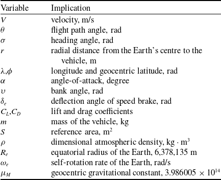
Table 1 is the statement of corresponding variable. In Equation (1), $ i=1$ represents the HGV as a leader and $ i=\mathrm{2,3},\cdots ,n$ represents the HGVs as followers; $ {\rho }_{i}$ is formulated as $ {\rho }_{i}={\rho }_{0}{e}^{-\frac{{h}_{i}}{{H}_{MCP}}}$ , where $ {h}_{i}={r}_{i}-{R}_{e}$ , $ {\rho }_{0}=1.225$ , $ {H}_{MCP}=7100$ ; the lift coefficient and drag coefficient can be expressed by $ {C}_{{L}_{i}}={C}_{{L}_{i}}^{\alpha }{\alpha }_{i}$ , $ {C}_{{D}_{i}}={C}_{{D}_{i}}^{{\alpha }_{i}^{2}}{\alpha }_{i}^{2}+{C}_{{D}_{i}}^{{\alpha }_{i}}{\alpha }_{i}+{C}_{{D}_{i}}^{0}+{C}_{{D}_{i}}^{{\delta }_{e}}{\delta }_{e,i}$ . The Coriolis force $ {C}_{V,i}$ , $ {C}_{\theta ,i}$ , $ {C}_{\sigma ,i}$ and centrifugal inertia force $ {C}_{\theta ,i}^{\mathrm{\text{'}}}$ , $ {C}_{\sigma ,i}^{\mathrm{\text{'}}}$ caused by the rotation of the earth are given by:

(2) \begin{align}\left\{\begin{array}{ll}{C}_{V,i}\,=\,{\omega }_{e}^{2}{r}_{i}\,\mathrm{c}\mathrm{o}\mathrm{s}{\phi }_{i}\left(\mathrm{s}\mathrm{i}\mathrm{n}{\theta }_{i}\,\mathrm{c}\mathrm{o}\mathrm{s}{\phi }_{i}-\mathrm{c}\mathrm{o}\mathrm{s}{\theta }_{i}\,\mathrm{c}\mathrm{o}\mathrm{s}{\sigma }_{i}\,\mathrm{s}\mathrm{i}\mathrm{n}{\phi }_{i}\right) {} \\ {C}_{\theta ,i}\,=\,\frac{{\omega }_{e}^{2}{r}_{i}\,\mathrm{c}\mathrm{o}\mathrm{s}{\phi }_{i}}{{V}_{i}}\left(\mathrm{c}\mathrm{o}\mathrm{s}{\theta }_{i}\,\mathrm{c}\mathrm{o}\mathrm{s}{\phi }_{i}+\mathrm{s}\mathrm{i}\mathrm{n}{\theta }_{i}\,\mathrm{c}\mathrm{o}\mathrm{s}{\sigma }_{i}\,\mathrm{s}\mathrm{i}\mathrm{n}{\phi }_{i}\right) {} \\ {C}_{\sigma ,i}\,=\,{\omega }_{e}^{2}{r}_{i}\frac{\mathrm{s}\mathrm{i}\mathrm{n}{\theta }_{i}\,\mathrm{s}\mathrm{i}\mathrm{n}{\phi }_{i}\,\mathrm{c}\mathrm{o}\mathrm{s}{}_{i}}{{V}_{i}\,\mathrm{c}\mathrm{o}\mathrm{s}{\theta }_{i}} {} \\ {C}_{\theta ,i}^{\mathrm{\text{'}}}\,=\,2{\omega }_{e}\,\mathrm{c}\mathrm{o}\mathrm{s}{\phi }_{i}\,\mathrm{s}\mathrm{i}\mathrm{n}{\sigma }_{i} {} \\ {C}_{\sigma ,i}^{\mathrm{\text{'}}}\,=\,-2{\omega }_{e}\left(\mathrm{c}\mathrm{o}\mathrm{s}{\phi }_{i}\,\mathrm{t}\mathrm{a}\mathrm{n}{\theta }_{i}\,\mathrm{c}\mathrm{o}\mathrm{s}{\sigma }_{i}-\mathrm{s}\mathrm{i}\mathrm{n}{\phi }_{i}\right)\end{array}\right.\end{align}

Table 1.

Nomenclature

Define $ {\eta }_{i,1}={\left[{r}_{i},{\lambda }_{i},{\phi }_{i}\right]}^{T}$ , $ {\eta }_{i,2}={\left[{V}_{i},{\theta }_{i},{\sigma }_{i}\right]}^{T}$ , ${u}_{i}={\left[-{\delta }_{e,i},{C}_{L,i}\mathrm{c}\mathrm{o}\mathrm{s}{\upsilon }_{i},{C}_{L,i}\mathrm{s}\mathrm{i}\mathrm{n}{\upsilon }_{i}\right]}^{T}$ , consider the effects of uncertainties and disturbances to which the system is subjected in engineering practice, we obtain the time-based system dynamics:

(3) \begin{align}\left\{\begin{array}{ll}{\dot{\eta }}_{i,1}={\mathrm{\Lambda }}_{i,1}\left({\bar{\eta}}_{i,1}\right)+{\mathrm{\Gamma }}_{i,1}\left({\bar{\eta}}_{i,1},{\eta }_{i,2}\right)+\mathrm{\Delta }{\delta }_{i,1}+{\zeta }_{i,1}\left(t\right)+\mathrm{\Delta }{\xi }_{i,1}\left(t\right) {} \\ {\dot{\eta }}_{i,2}={\mathrm{\Lambda }}_{i,2}\left({\bar{\eta}}_{i,2}\right)+{\mathrm{\Gamma }}_{i,2}\left({\bar{\eta}}_{i,2},{u}_{i}\right)+\mathrm{\Delta }{\delta }_{i,2}+\mathrm{\Delta }{\xi }_{i,2}\left(t\right) {} \\ {\varpi }_{i}={\eta }_{i,1},i=\mathrm{2,3},n\end{array}\right.\end{align}

where $ {\bar{\eta}}_{i,j}={\eta }_{i,1},\cdots ,{\eta }_{i,j}$ . In Equation (3), $ {\mathrm{\Lambda }}_{i,1}$ and $ {\mathrm{\Lambda }}_{i,2}$ are known nonlinear functions whose form are shown in Equations (4) and (5), $ {\mathrm{\Gamma }}_{i,1}$ and $ {\mathrm{\Gamma }}_{i,2}$ are non-affine functions of the form shown in Equations (6) and (7)

(4) \begin{align}{\mathrm{\Lambda }}_{i,1}=0\end{align}

(5) \begin{align}{\mathrm{\Lambda }}_{i,2}=\left[\begin{array}{c}-\frac{{\mu }_{M}}{{\left({\eta }_{i,{1}_{\left(31\right)}}\right)}^{2}}\mathrm{s}\mathrm{i}\mathrm{n}\,{\eta }_{i,{2}_{\left(32\right)}}+{C}_{V,i}\\ \left(\frac{{\eta }_{i,{2}_{\left(31\right)}}}{{\eta }_{,{1}_{\left(31\right)}}}-\frac{{\mu }_{M}}{{\eta }_{i,{2}_{\left(31\right)}}{\left({\eta }_{i,{1}_{\left(31\right)}}\right)}^{2}}\right)\mathrm{c}\mathrm{o}\mathrm{s}\,{\eta }_{i,{2}_{\left(32\right)}}+{C}_{\theta ,i}+{C}_{\theta ,i}^{\mathrm{\text{'}}}\\ \frac{{\eta }_{i,{2}_{\left(31\right)}}\mathrm{c}\mathrm{o}\mathrm{s}\,{\eta }_{i,{2}_{\left(32\right)}}\mathrm{s}\mathrm{i}\mathrm{n}\,{\eta }_{i,{2}_{\left(33\right)}}\mathrm{t}\mathrm{a}\mathrm{n}\,{\eta }_{i,{1}_{\left(33\right)}}}{{\eta }_{i,{1}_{\left(31\right)}}}+{C}_{\sigma ,i}+{C}_{\sigma ,i}^{\mathrm{\text{'}}}\end{array}\right]\end{align}

(6) \begin{align}{\mathrm{\Gamma }}_{i,1}={\left[\begin{array}{lll}{{\eta }_{i,{2}_{\left(31\right)}}}_{i}\,\mathrm{s}\mathrm{i}\mathrm{n}\,{\eta }_{i,{2}_{\left(32\right)}}\,\, {} \frac{{\eta }_{i,{2}_{\left(31\right)}}\mathrm{c}\mathrm{o}\mathrm{s}\,{\eta }_{i,{2}_{\left(32\right)}}\mathrm{s}\mathrm{i}\mathrm{n}\,{\eta }_{i,{2}_{\left(33\right)}}}{{\eta }_{i,{1}_{\left(31\right)}}\mathrm{c}\mathrm{o}\mathrm{s}\,{\eta }_{i,{1}_{\left(33\right)}}}\,\, {} \frac{{\eta }_{i,{2}_{\left(31\right)}}\mathrm{c}\mathrm{o}\mathrm{s}\,{\eta }_{i,{2}_{\left(32\right)}}\mathrm{c}\mathrm{o}\mathrm{s}\,{\eta }_{i,{2}_{\left(33\right)}}}{{\eta }_{i,{1}_{\left(31\right)}}}\end{array}\right]}^{T}\end{align}

(7) \begin{align}{\mathrm{\Gamma }}_{i,2}=\left[\begin{array}{c}\mathrm{t}\mathrm{a}\mathrm{n}\mathrm{h}\left({u}_{{i}_{\left(31\right)}}\right)+\frac{\left({C}_{{D}_{i}}^{{\alpha }_{i}^{2}}{\alpha }_{i}^{2}+{C}_{{D}_{i}}^{{\alpha }_{i}}{\alpha }_{i}+{C}_{{D}_{i}}^{0}+{C}_{{D}_{i}}^{{\delta }_{e}}{u}_{{i}_{\left(31\right)}}\right){\rho }_{i}{\left({\eta }_{i,{2}_{\left(31\right)}}\right)}^{2}{S}_{i}}{2{m}_{i}}\\ \mathrm{t}\mathrm{a}\mathrm{n}\mathrm{h}\left({u}_{{i}_{\left(31\right)}}\right)+\frac{{u}_{{i}_{\left(32\right)}}{\rho }_{i}{\eta }_{i,{2}_{\left(31\right)}}{S}_{i}}{2{m}_{i}}\\ \mathrm{t}\mathrm{a}\mathrm{n}\mathrm{h}\left({u}_{{i}_{\left(31\right)}}\right)+\frac{{u}_{{i}_{\left(33\right)}}{\rho }_{i}{\eta }_{i,{2}_{\left(31\right)}}{S}_{i}}{2{m}_{i}\mathrm{c}\mathrm{o}\mathrm{s}{\eta }_{i,{2}_{\left(32\right)}}}\\ \end{array}\right]\\[-6pt]\nonumber\end{align}

Remark 3. $ {\zeta }_{i,1}\left(t\right)$ is the vehicle position measurement deviation at the initial moment. Then $ {\zeta }_{i,1}\left(t\right)$ can be formulated as follows:

(8) \begin{align}{\zeta }_{i,1}\left(t\right)=\left\{\begin{array}{lll}{\left[\mathrm{\Delta }{h}_{0},\mathrm{\Delta }{\lambda }_{0},\mathrm{\Delta }{\varphi }_{0}\right]}^{T},t={t}_{0} {} {} \\ {0}^{3\times 1},t\ne {t}_{0}\end{array}\right.\end{align}

We have observed that the system (3) exhibit non-affine behaviour, distinguishing them from typical affine systems. In affine systems, control inputs appear linearly and are separable from state-dependent terms. However, in hypersonic glide vehicle (HGV) dynamics, control inputs $ {u}_{i}$ are nonlinearly coupled with system states $ {\eta }_{i,1}$ , $ {\eta }_{i,2}$ . This includes high-order nonlinearities arising from dependencies on factors such as the angle-of-attack, Mach number and altitude. To address the issue of state-control coupling, we add an additional auxiliary differential equation $ {\dot{u}}_{i}={u}_{fi}$ to the Equation (3). Define $ {\eta }_{i,3}={u}_{i}$ , rewrite the feedback system (3) as follows

(9) \begin{align}\left\{\begin{array}{ll}{\dot{\eta }}_{i,1}={\mathrm{\Lambda }}_{i,1}\left({\bar{\eta}}_{i,1}\right)+{\mathrm{\Gamma }}_{i,1}\left({\bar{\eta}}_{i,1},{\eta }_{i,2}\right)+\mathrm{\Delta }{\delta }_{i,1}+{\zeta }_{i,1}\left(t\right)+\mathrm{\Delta }{\xi }_{i,1}\left(t\right) {} \\ {\dot{\eta }}_{i,2}={\mathrm{\Lambda }}_{i,2}\left({\bar{\eta}}_{i,2}\right)+{\mathrm{\Gamma }}_{i,2}\left({\bar{\eta}}_{i,2},{\eta }_{i,3}\right)+\mathrm{\Delta }{\delta }_{i,2}+\mathrm{\Delta }{\xi }_{i,2}\left(t\right) {} \\ {\dot{\eta }}_{i,3}={u}_{fi} {} \\ {\varpi }_{i}={\eta }_{i,1},i=\mathrm{2,3},n\end{array}\right.\end{align}

Obviously, the multi-HGV consensus tracking system is a nonlinear three-order feedback system. Nevertheless, in contrast to the standard back-stepping technique, new actions need be made to handle the effects of disturbances and uncertainties. The control goal is to make the output tracking error of followers exponentially converge to a small neighbourhood ensuring the global boundary of all closed-loop signals in the meanwhile. The framework of the proposed consensus controller for multi-HGV system is presented in Figure 1.

Figure 1.

The framework of the proposed consensus controller for multi-HGV system.

Following assumptions are proposed to implement controller:

Assumption 6. For functions in non-affine form, there have positive lower bound $ \underset{-}{\Gamma }$ and upper bound $ \bar{\Gamma}$ satisfying the following form:

(10) \begin{align}0\lt\underset{-}{\mathrm{\Gamma }}\le \Bigg\|\frac{\partial {\mathrm{\Gamma }}_{i,\,j}\left({\bar{\eta}}_{i,\,j},{\eta }_{i,\,j+1}\right)}{\partial {\eta }_{i,k}}\Bigg\|\le \bar{\mathrm{\Gamma }}\lt\infty \end{align}

At the end of this section, the following lemmas are put forward, which will be utilised soon afterwards.

Lemma 1. [Reference Xie and Xie31] For any $ x\in {\mathbb{R}}^{n}$ , if there exist positive constants $ \chi $ , $ \delta $ , positive definite function $ \Phi \left(x,t\right)$ and class kappa function $ {\mathcal{K}}_{1}$ , $ {\mathcal{K}}_{2}$ satisfying: $ {\mathcal{K}}_{1}\left(\left|x\right|\right)\le \Phi \left(x,t\right)\le {\mathcal{K}}_{2}\left(\left|x\right|\right)$ and $ \dot{\Phi }\left(x,t\right)\le -\chi \Phi \left(x,t\right)+\delta $ . Then, there is a unique strong solution of the system that:

(11) \begin{align}\mathrm{\Phi }\left(x,t\right)\le \mathrm{\Phi }\left({x}_{0}\right){e}^{-\chi t}+\frac{\delta }{\chi },\forall t \gt{t}_{0}\end{align}

Lemma 2. [Reference Polycarpou and Ioannou32] For any $ \varepsilon \gt0$ and $ x\in \mathbb{R}$ , we have

(12) \begin{align}0\le \left|x\right|-x\,\mathrm{t}\mathrm{a}\mathrm{n}\mathrm{h}(x/\zeta )\le \iota \varepsilon \end{align}

where $ \iota $ is a constant satisfying $ \iota ={e}^{-(\iota +1)}$ , $ \iota =0.2785$ .

2.2 Graph theory

In a multi-agent system, a communication network between agents can be described by a graph $ \mathcal{G}=\left(\mathcal{V},\varepsilon ,\mathcal{A}\right)$ , where $ \mathcal{V}=\left\{\mathrm{1,2},\dots ,n\right\}$ is set of nonempty nodes, $ \varepsilon =\left\{\left({n}_{i},{n}_{j}\right)\right\}\in \mathcal{V}\times \mathcal{V}$ represents the set of edges, $ \mathcal{A}=\left[{a}_{ij}\right]\in {\mathbb{R}}^{n\times n}$ is adjacency matrix. If $ \left({n}_{i},{n}_{j}\right)\in \varepsilon $ , $ {a}_{ij}\gt0$ , then the agent $ i$ can pass information to agent $ j$ . If $ \left({n}_{i},{n}_{j}\right)\notin \varepsilon $ , then $ {a}_{ij}=0$ . We assume that agents do not have access to information about themselves, which means $ {a}_{ii}=0$ . For undirected graphs, the adjacency matrix is symmetric meaning $ {a}_{ij}={a}_{ji}\gt0$ . For any directed graph, the adjacency matrix is asymmetric.

The degree matrix $ \mathcal{D}=diag\left({d}_{1},{d}_{2},\dots ,{d}_{n}\right)\in {\mathbb{R}}^{n\times n}$ of graph $ \mathcal{G}$ represents the sum of the outdegree and indegree of a node. Note that $ \mathcal{D}$ is a diagonal array and the diagonal elements are $ {d}_{i}=\sum _{j\in {N}_{i}}{a}_{ij},i=\mathrm{1,2},\dots ,n$ . Define the Laplacian matrix as $ \mathcal{L}=\mathcal{D}-\mathcal{A}$ , we have

(13) \begin{align}{\mathcal{L}}_{ij}=\left\{\begin{array}{ll}\mathop\sum\limits_{j\in {n}_{i}}{a}_{ij},i=j {} \\ -{a}_{ij},i\ne j\end{array}\right.\end{align}

Consider the information sharing between leaders and followers to be unidirectional, i.e., the leaders can pass information to the followers, but the information of followers cannot influence the leaders. Define $ \mathcal{S}=diag\left({s}_{1},{s}_{2},\dots ,{s}_{n}\right)$ , note that $ {s}_{i}=1$ when followers can get information from the leader, otherwise $ {s}_{i}=0$ . Denote $ \mathcal{H}=\mathcal{L}+\mathcal{S}$ the communication topology matrix, which represents the information transmission relation between leaders and followers. When at least one follower can get information from the leader and the undirected graph is connected, $ \mathcal{H}\gt\gt0$ .

2.3 Radial basis function neural network

In this section, the RBFNN can approximate an arbitrary smooth continuous function with arbitrary accuracy is introduced. Define $ l$ -dimensional input vector as $ x\in {\mathbb{R}}^{l}$ , weight vector as $ \mathrm{\Theta }\in {\mathbb{R}}^{p\times m}$ , Gaussian basis function vector as $ S\left(x\right)={\left[{S}_{1}\left(x\right),\dots ,{S}_{p}\left(x\right)\right]}^{T}$ , $ {\mathrm{\Phi }}_{j}\left(x\right)={e}^{-\frac{(x-{\mu }_{j}{)}^{2}}{2{{\sigma }_{j}}^{2}}},\,j=1,\dots ,p$ , where $ {\mu }_{j}$ represents the centre of the basis function, $ {\sigma }_{j}$ is the width of the Gaussian basis function. The expression of the RBFNN is denoted as:

(14) \begin{align}f={\mathrm{\Theta }}^{\mathrm{*}T}S\left(x\right)+\varepsilon \left(x\right)\end{align}

where $ {\mathrm{\Theta }}^{\mathrm{*}}$ is the ideal weight vector, the basic functions satisfy $ \left|\right|S\left(x\right)\left|\right|\le {S}_{M}$ , $ \varepsilon $ is the approximation error satisfying $ \|\varepsilon \|\le {\varepsilon }_{M}$ , $ \|\dot{\varepsilon }\|\le {\varepsilon }_{m}$ .

3.1 Tight-formation configuration design

Consider the effects of aerodynamic disturbances, communication constraints and violently time-varying environments during the clustering of HGVs, rational formation alignment must be employed. Drawing on the sharp angle ‘V’ formation of geese [Reference Li, Wang, Shen, Peng and Wang33], the hypersonic vehicles cluster adopts the ‘leader-follower’ formation shown in Figure 2.

Figure 2.

HGVs cluster formation configuration.

From Figure 2, we notice that during the whole formation process, follower-2 and follower-3 are at the left-rear and right-rear of leader-1, respectively, while maintaining a lateral relative distance $ \mathrm{\Delta }W$ , longitudinal relative distance $ \mathrm{\Delta }L$ , vertical relative distance $ \mathrm{\Delta }H$ from the leader. Follower-4 is located directly above leader-1 while maintaining a vertical relative distance $ \mathrm{\Delta }H$ from the leader during flight.

Obviously the first-order consensus tracking error in multi-HGV system (9) is $ {\eta }_{i,1}={\left[{r}_{i},{\lambda }_{i},{\phi }_{i}\right]}^{T}$ rather than $ {\left[\mathrm{\Delta }{H}_{i},\mathrm{\Delta }{L}_{i},\mathrm{\Delta }{W}_{i}\right]}^{T}$ . Thus, we reestablish a generalised equatorial coordinate system $ M$ [Reference Xie, Liu, Liu, Tang and Zheng34] to replace the geocentric coordinate system. By using the transformation matrix between the $ E$ -coordinate system and the $ M$ -coordinate system, we can convert longitudinal, lateral and vertical relative distances into latitude, longitude and height deviations.

As shown in Figure 3, a new generalised equatorial plane $ P$ is firstly determined by denoting the current position $ \left[{r}_{1},{\lambda }_{1},{\phi }_{1}\right]$ of leader as gliding departure point $ I$ and current heading angle $ {\sigma }_{1}$ as the azimuthal angle. Then we define a generalised equatorial coordinate system $ {O}_{E}-{X}_{M}{Y}_{M}{Z}_{M}$ : $ {O}_{E}$ is the centre of the Earth, $ {O}_{E}{X}_{M}$ -axis follows the direction of the geocentric vector path at point $ I$ . $ {O}_{E}{Y}_{M}$ -axis is perpendicular to the $ {O}_{E}{X}_{M}$ -axis in the plane $ P$ and points in the direction of the leader’s flight. $ {O}_{E}{Z}_{M}$ -axis forms a right-handed system with the $ {O}_{E}{X}_{M}$ -axis and $ {O}_{E}{Y}_{M}$ -axis $ M$ . The transformation matrix $ {G}_{M}^{E}$ between the coordinate system $ M$ and $ E$ is described in Equation (15):

(15) \begin{align}{G}_{M}^{E}=\left[\begin{array}{lll}\mathrm{c}\mathrm{o}\mathrm{s}{\phi }_{1}\,\mathrm{c}\mathrm{o}\mathrm{s}{\lambda }_{1}\quad {} -\mathrm{s}\mathrm{i}\mathrm{n}{\sigma }_{1}\,\mathrm{s}\mathrm{i}\mathrm{n}{\lambda }_{1}-\mathrm{c}\mathrm{o}\mathrm{s}{\sigma }_{1}\,\mathrm{s}\mathrm{i}\mathrm{n}{\phi }_{1}\,\mathrm{c}\mathrm{o}\mathrm{s}{\lambda }_{1}\quad\mathrm{c}\mathrm{o}\mathrm{s}{\sigma }_{1}\,\mathrm{s}\mathrm{i}\mathrm{n}{\lambda }_{1}-\mathrm{s}\mathrm{i}\mathrm{n}{\sigma }_{1}\,\mathrm{s}\mathrm{i}\mathrm{n}{\phi }_{1}\,\mathrm{c}\mathrm{o}\mathrm{s}{\lambda }_{1}\,\\ \mathrm{c}\mathrm{o}\mathrm{s}{\phi }_{1}\,\mathrm{s}\mathrm{i}\mathrm{n}{\lambda }_{1}\quad\quad\mathrm{s}\mathrm{i}\mathrm{n}{\sigma }_{1}\,\mathrm{c}\mathrm{o}\mathrm{s}{\lambda }_{1}-\mathrm{c}\mathrm{o}\mathrm{s}{\sigma }_{1}\,\mathrm{s}\mathrm{i}\mathrm{n}{\phi }_{1}\,\mathrm{s}\mathrm{i}\mathrm{n}{\lambda }_{1}\quad-\mathrm{c}\mathrm{o}\mathrm{s}{\sigma }_{1}\,\mathrm{c}\mathrm{o}\mathrm{s}{\lambda }_{1}-\mathrm{s}\mathrm{i}\mathrm{n}{\sigma }_{1}\,\mathrm{s}\mathrm{i}\mathrm{n}{\phi }_{1}\,\mathrm{s}\mathrm{i}\mathrm{n}{\lambda }_{1}\,\\ \quad\mathrm{s}\mathrm{i}\mathrm{n}{\phi }_{1}\quad\quad\quad\quad\quad\quad\quad\mathrm{c}\mathrm{o}\mathrm{s}{\sigma }_{1}\,\mathrm{c}\mathrm{o}\mathrm{s}{\phi }_{1}\quad\quad\quad\quad\quad\quad\quad\quad\quad\,\,\,\,\mathrm{s}\mathrm{i}\mathrm{n}{\sigma }_{1}\,\mathrm{c}\mathrm{o}\mathrm{s}{\phi }_{1}\,\end{array}\right]\end{align}

Figure 3.

M-Coordinate diagram.

Consider the earth as a sphere with radius $ {R}_{e}$ and the location of follower- $ i$ in coordinate system $ M$ as $ \left({r}_{M,i},{\lambda }_{M,i},{\phi }_{M,i}\right),i=\mathrm{2,3},4$ , we denote the lateral relative distance, longitudinal relative distance, vertical relative distance between follower- $ i$ and the leader as $ \mathrm{\Delta }{W}_{i}={R}_{e}{\phi }_{M,i}$ , $ \mathrm{\Delta }{L}_{i}={R}_{e}{\lambda }_{M,i}$ , $ \mathrm{\Delta }{H}_{i}={r}_{M,i}-{r}_{1}$ respectively. Define the relative position of follower $ i$ and leader in the coordinate system $ E$ as $ \left(\mathrm{\Delta }{r}_{i},\mathrm{\Delta }{\lambda }_{i},\mathrm{\Delta }{\phi }_{i}\right)$ , then the conversion relationship between $ \left(\mathrm{\Delta }{r}_{i},\mathrm{\Delta }{\lambda }_{i},\mathrm{\Delta }{\phi }_{i}\right)$ and $ \left(\mathrm{\Delta }{W}_{i},\mathrm{\Delta }{L}_{i},\mathrm{\Delta }{H}_{i}\right)$ is given by

(16) \begin{align}\left[\begin{array}{c}\mathrm{\Delta }{r}_{i}\,\mathrm{c}\mathrm{o}\mathrm{s}\,\mathrm{\Delta }{\phi }_{i}\,\mathrm{c}\mathrm{o}\mathrm{s}\,\mathrm{\Delta }{\lambda }_{i}\\ \mathrm{\Delta }{r}_{i}\,\mathrm{c}\mathrm{o}\mathrm{s}\,\mathrm{\Delta }{\phi }_{i}\,\mathrm{s}\mathrm{i}\mathrm{n}\,\mathrm{\Delta }{\lambda }_{i}\\ \mathrm{\Delta }{r}_{i}\,\mathrm{s}\mathrm{i}\mathrm{n}\,\mathrm{\Delta }{\phi }_{i}\\ \end{array}\right]={G}_{M}^{E}\left[\begin{array}{c}\left(\mathrm{\Delta }{H}_{i}+{r}_{1}\right)\,\mathrm{c}\mathrm{o}\mathrm{s}\,\frac{\mathrm{\Delta }{W}_{i}}{{R}_{e}}\,\mathrm{c}\mathrm{o}\mathrm{s}\,\frac{\mathrm{\Delta }{L}_{i}}{{R}_{e}}\\ \left(\mathrm{\Delta }{H}_{i}+{r}_{1}\right)\,\mathrm{c}\mathrm{o}\mathrm{s}\,\frac{\mathrm{\Delta }{W}_{i}}{{R}_{e}}\,\mathrm{s}\mathrm{i}\mathrm{n}\,\frac{\mathrm{\Delta }{L}_{i}}{{R}_{e}}\\ \left(\mathrm{\Delta }{H}_{i}+{r}_{1}\right)\,\mathrm{s}\mathrm{i}\mathrm{n}\,\frac{\mathrm{\Delta }{W}_{i}}{{R}_{e}}\\ \end{array}\right]\triangleq \left[\begin{array}{l}{\kappa }_{1}\\ {\kappa }_{2}\\ {\kappa }_{3}\end{array}\right]\end{align}

Thus, we have:

(17) \begin{align}\mathrm{\Delta }{r}_{i}=\mathrm{\Delta }{H}_{i}+{r}_{1},\mathrm{\Delta }{\lambda }_{i}=\mathrm{a}\mathrm{r}\mathrm{c}\mathrm{t}\mathrm{a}\mathrm{n}\left(\frac{{\kappa }_{2}}{{\kappa }_{1}}\right),\mathrm{\Delta }{\phi }_{i}=\mathrm{a}\mathrm{r}\mathrm{c}\mathrm{t}\mathrm{a}\mathrm{n}\left(\frac{{\kappa }_{3}}{\sqrt{{\kappa }_{1}^{2}+{\kappa }_{2}^{2}}}\right)\end{align}

In summary, the position of the follower- $ i$ in the $ E$ coordinate system is $ \left({r}_{i},{\lambda }_{i},{\phi }_{i}\right)=\left({r}_{1},{\lambda }_{1},{\phi }_{1}\right)+\left(\mathrm{\Delta }{r}_{i},\mathrm{\Delta }{\lambda }_{i},\mathrm{\Delta }{}_{i}\right)$ .

3.2 Controller design

Step 1: Define the position tracking error for the follower- $ i$ as $ {z}_{i,1}=\sum _{k=2}^{n}{a}_{ik}\left({y}_{i,d}-{y}_{k,d}\right)+{s}_{i}\left({y}_{i,d}-{y}_{1}\right)$ , where $ {y}_{i,d}$ , $ {y}_{k,d}$ represent virtual flight trajectory. Then $ {z}_{1}={\left[{z}_{\mathrm{2,1}},{z}_{\mathrm{3,1}},\cdots ,{z}_{n,1}\right]}^{T}$ can be summarised as:

(18) \begin{align}{z}_{1}=\left(\mathcal{L}+\mathcal{S}\right)e\end{align}

where $ \mathcal{L}$ is calculated with reference to Equation (13), $ \mathcal{S}=diag\left({s}_{1},{s}_{2},\dots ,{s}_{n}\right)$ , $ e={\left[{y}_{2,d}-{y}_{1},{}{y}_{3,d}-{y}_{1},\cdots ,{y}_{n,d}-{y}_{1}\right]}^{T}$ is the actual tracking error.

Combining Equations (9) and (18), we have

(19) \begin{align}\begin{array}{ll}{\dot{z}}_{1}&=\left(\mathrm{L}+\mathrm{S}\right)\dot{e}\\&=\left(\mathrm{L}+\mathrm{S}\right)\left[\begin{array}{llllllllllllllllllll}{\dot{\eta }}_{i,1}-{\dot{y}}_{1} \\ \quad\,\,\vdots \\ {\dot{\eta }}_{n,1}-{\dot{y}}_{1}\end{array}\right]\\&=\left(\mathrm{L}+\mathrm{S}\right)\left[\begin{array}{llllllllllllllllllll}{\mathrm{\Lambda }}_{i,1}\left({\bar{\eta}}_{i,1}\right)+{\mathrm{\Gamma }}_{i,1}\left({\bar{\eta}}_{i,1},{\eta }_{i,2}\right)+\mathrm{\Delta }{\delta }_{i,1}+{\zeta }_{i,1}\left(t\right)+\mathrm{\Delta }{\xi }_{i,1}\left(t\right)-{\dot{y}}_{1}\\ \quad\quad\quad\quad\quad\quad\quad\quad\quad\quad\quad\quad \vdots\\ {\mathrm{\Lambda }}_{n,1}\left({\bar{\eta}}_{n,1}\right)+{\mathrm{\Gamma }}_{n,1}\left({\bar{\eta}}_{n,1},{\eta }_{n,2}\right)+\mathrm{\Delta }{\delta }_{n,1}+{\zeta }_{n,1}\left(t\right)+\mathrm{\Delta }{\xi }_{n,1}\left(t\right)-{\dot{y}}_{1}\end{array}\right]\end{array}\end{align}

Define $ \mathrm{\Delta }{\bar{\delta}}_{i,1}=\|\mathrm{\Delta }{\delta }_{i,1}\|$ , RBFNN is exploited to compensate the deviation induced by unknown nonlinear function $ \mathrm{\Delta }{\delta }_{i,1}$ :

(20) \begin{align}\mathrm{\Delta }{\bar{\delta }}_{i,1}={\mathrm{\Theta }}_{i,1}^{T}{\mathrm{\Phi }}_{i,1}\left({\bar{\eta }}_{i,1}\right)+{\varepsilon }_{i,1}\left({\bar{\eta }}_{i,1}\right)\end{align}

Define $ \mathrm{\Delta }{\widehat{\delta }}_{i,1}={\widehat{\mathrm{\Theta }}}_{i,1}^{T}{\mathrm{\Phi }}_{i,1}\left({\bar{\eta}}_{i,1}\right)$ , where $ {\widehat{\mathrm{\Theta }}}_{i,1}$ is the estimation of $ {\mathrm{\Theta }}_{i,1}$ . Then the estimation error $ \tilde{\Theta}_{i,1}$ can be written as $ \tilde{\Theta}_{i,1}={\widehat{\mathrm{\Theta }}}_{i,1}-{\mathrm{\Theta }}_{i,1}$ .

Define $ {D}_{i,1}=\mathrm{s}\mathrm{u}{\mathrm{p}}_{t\ge 0}\big\|\left({\zeta }_{i,1}+\mathrm{\Delta }{\xi }_{i,1}+{\varepsilon }_{i,1}\right)\big\|$ , then the hyperbolic tangent function is used to compensate the interference boundary estimator based on Lemma 2. Denote $ {\widehat{D}}_{i,1}$ as the estimates of $ {D}_{i,1}$ , then the estimation error $ {D}_{i,1}$ can be computed as $ \tilde{D}_{i,1}={\widehat{D}}_{i,1}-{D}_{i,1}$ .

The virtual control signal $ {\eta }_{i,2c}$ of the follower- $ i$ in the first order subsystem is devised as follows:

(21) \begin{align}{\eta }_{i,2c}=-\left({c}_{i,1}+\frac{1}{2}\right){z}_{i,1}-{\widehat{\mathrm{\Theta }}}_{i,1}^{T}{\mathrm{\Phi }}_{i,1}-{\widehat{D}}_{i,1}\mathrm{t}\mathrm{a}\mathrm{n}\mathrm{h}\left(\frac{{z}_{i,1}}{{\varepsilon }_{{D}_{i,1}}}\right)-{\mathrm{\Lambda }}_{i,1}+{\dot{y}}_{1,d}\end{align}

where $ {c}_{i,1}$ is a positive parameter that need to be designed.

Herein, a new variable $ {\eta }_{i,2d}$ is presented in the following form:

(22) \begin{align}\tau {\dot{\eta }}_{i,2d}+{\eta }_{i,2d}={\eta }_{i,2c},{\eta }_{i,2d}\left(0\right)=0,{\eta }_{i,2c}\left(0\right)=0\end{align}

where $ \tau $ is a positive constant.

Define the filter error as $ {\varsigma }_{i,2}={\eta }_{i,2d}-{\eta }_{i,2c}$ , the second order subsystem error as $ {z}_{i,2}={\mathrm{\Gamma }}_{i,1}-{\eta }_{i,2d}$ . Substituting Equations (21) and (22) into Equation (19), we can get following dynamic equations:

(23) \begin{align}{\dot{z}}_{1}=\left(\mathcal{L}+\mathcal{S}\right)\left[\begin{array}{c}-\left({c}_{i,1}+\frac{1}{2}\right){z}_{i,1}+{z}_{,2}+{\varsigma }_{i,2}-\tilde{\Theta}_{i,1}^{T}{\mathrm{\Phi }}_{i,1}+\left({\xi }_{i,1}+{\varepsilon }_{i,1}-{\widehat{D}}_{i,1}\mathrm{t}\mathrm{a}\mathrm{n}\mathrm{h}\left(\frac{{z}_{i,1}}{{\varepsilon }_{{D}_{i,1}}}\right)\right)\\ \vdots\\ -\left({c}_{n,1}+\frac{1}{2}\right){z}_{n,1}+{z}_{n,2}+{\varsigma }_{n,2}-\tilde{\Theta}_{n,1}^{T}{\mathrm{\Phi }}_{n,1}+\left({\xi }_{n,1}+{\varepsilon }_{n,1}-{\widehat{D}}_{n,1}\mathrm{t}\mathrm{a}\mathrm{n}\mathrm{h}\left(\frac{{z}_{n,1}}{{\varepsilon }_{{D}_{n,1}}}\right)\right)\end{array}\right]\end{align}

By using the following Lyapunov function candidate

(24) \begin{align}{\mathrm{{\rm Y}}}_{1}=\frac{1}{2}{e}^{T}\left(\mathcal{L}+\mathcal{S}\right)e+\frac{1}{2}\sum _{i=2}^{n}{\varsigma }_{i,2}^{2}+\frac{1}{2{f}_{i,1}}\sum _{i=2}^{n}\tilde{\Theta}_{i,1}^{T}\tilde{\Theta}_{i,1}+\frac{1}{2{b}_{i,1}}\sum _{i=2}^{n}\tilde{D}_{i,1}^{2}\end{align}

where $ {f}_{i,1}$ , $ {b}_{i,1}$ are the gains of the adaptive laws.

Hence, we take the derivative of $ {\mathrm{{\rm Y}}}_{1}$ combining Equation (23) as

(25) \begin{align}\begin{array}{ll}{\dot{\mathrm{{\rm Y}}}}_{1} {} =-\mathop\sum\limits_{i=2}^{n}\left({c}_{i,1}+\frac{1}{2}\right){z}_{i,1}^{2}+\mathop\sum\limits_{i=2}^{n}{z}_{i,1}{z}_{i,2}+\mathop\sum\limits_{i=2}^{n}{z}_{i,1}{\varsigma }_{i,2}-\mathop\sum\limits_{i=2}^{n}{z}_{i,1}\tilde{\Theta}_{\mathrm{1,1}}^{T}{\mathrm{\Phi }}_{i,1}+\frac{1}{{f}_{i,1}}\mathop\sum\limits_{i=2}^{n}\tilde{\Theta}_{i,1}^{T}{\dot{\widehat{\mathrm{\Theta }}}}_{i,1}\\ {} +\frac{1}{{b}_{i,1}}\mathop\sum\limits_{i=2}^{n}\tilde{D}_{i,1}{\dot{\widehat{D}}}_{i,1}+\mathop\sum\limits_{i=2}^{n}{z}_{i,1}\left({\varepsilon }_{i,1}+{\xi }_{i,1}-{\widehat{D}}_{i,1}\mathrm{t}\mathrm{a}\mathrm{n}\mathrm{h}\left(\frac{{z}_{i,1}}{{\varepsilon }_{{D}_{i,1}}}\right)\right)-\mathop\sum\limits_{i=2}^{n}\frac{{\varsigma }_{i,2}^{2}}{\tau }-\mathop\sum\limits_{i=2}^{n}{\varsigma }_{i,2}{\dot{\eta }}_{i,2c}\end{array}\end{align}

The update law of adaptive parameter is designed as:

(26) \begin{align}{\dot{\widehat{D}}}_{i,1}={b}_{i,1}\left({z}_{i,1}\mathrm{t}\mathrm{a}\mathrm{n}\mathrm{h}\left(\frac{{z}_{i,1}}{{\varepsilon }_{{D}_{i,1}}}\right)-{\mu }_{{D}_{i,1}}{\widehat{D}}_{i,1}\right)\end{align}

The update law of network weight is designed as:

(27) \begin{align}{\dot{\widehat{\mathrm{\Theta }}}}_{i,1}={f}_{i,1}\left({\mathrm{\Phi }}_{i,1}{z}_{i,1}-{\mu }_{{\mathrm{\Theta }}_{i,1}}{\widehat{\mathrm{\Theta }}}_{i,1}\right)\end{align}

By substituting adaptive parameter update law (26) and network weight update law (27) into Equation (25), we get

(28) \begin{align}\begin{array}{ll}{\dot{\mathrm{{\rm Y}}}}_{1} {} =-\mathop\sum\limits_{i=2}^{n}\left({c}_{i,1}+\frac{1}{2}\right){z}_{i,1}^{2}+\mathop\sum\limits_{i=2}^{n}{z}_{i,1}{z}_{i,2}+\mathop\sum\limits_{i=2}^{n}{z}_{i,1}{\varsigma }_{i,2}+\mathop\sum\limits_{i=2}^{n}{z}_{i,1}\left({\varepsilon }_{i,1}+{\xi }_{i,1}-{\widehat{D}}_{i,1}\mathrm{t}\mathrm{a}\mathrm{n}\mathrm{h}\left(\frac{{z}_{i,1}}{{\varepsilon }_{{D}_{i,1}}}\right)\right)\\ {} -\mathop\sum\limits_{i=2}^{n}\frac{{\varsigma }_{i,2}^{2}}{\tau }-\mathop\sum\limits_{i=2}^{n}{\varsigma }_{i,2}{\dot{x}}_{i,2c}-\mathop\sum\limits_{i=2}^{n}{\mu }_{{\mathrm{\Theta }}_{i,1}}\tilde{\Theta}_{i,1}^{T}{\widehat{\mathrm{\Theta }}}_{i,1}+\mathop\sum\limits_{i=2}^{n}\tilde{D}_{i,1}{z}_{i,1}\mathrm{t}\mathrm{a}\mathrm{n}\mathrm{h}\left(\frac{{z}_{i,1}}{{\varepsilon }_{{D}_{i,1}}}\right)-\mathop\sum\limits_{i=2}^{n}{\mu }_{{D}_{i,1}}\tilde{D}_{i,1}{\widehat{D}}_{i,1}\end{array}\end{align}

Based on Lemma 2, the inequality is obtained

(29) \begin{align}{z}_{i,1}\left({\varepsilon }_{i,1}+{\xi }_{i,1}-{\widehat{D}}_{i,1}\mathrm{t}\mathrm{a}\mathrm{n}\mathrm{h}\left(\frac{{z}_{i,1}}{{\varepsilon }_{{D}_{i,1}}}\right)\right)\le -{z}_{i,1}\tilde{D}_{i,1}\mathrm{t}\mathrm{a}\mathrm{n}\mathrm{h}\left(\frac{{z}_{i,1}}{{\varepsilon }_{{D}_{i,1}}}\right)+\iota {\varepsilon }_{{D}_{i,1}}\end{align}

From Young’s inequality, it is easy to get that

(30) \begin{align}\begin{array}{ll}{\widehat{D}}_{i,1}\tilde{D}_{i,1} {} \le \frac{1}{2}{D}_{i,1}^{2}-\frac{1}{2}\tilde{D}_{i,1}^{2}\\[3pt] \tilde{\Theta}_{i,1}^{T}{\widehat{\mathrm{\Theta }}}_{i,1} {} \le \frac{1}{2}{\mathrm{\Theta }}_{i,1}^{T}{\mathrm{\Theta }}_{i,1}-\frac{1}{2}\tilde{\Theta}_{i,1}^{T}\tilde{\Theta}_{i,1}\\[3pt] -{\varsigma }_{i,2}{\dot{\eta }}_{i,2c} {} \le \frac{1}{2\tau }{\varsigma }_{i,2}^{2}+\frac{1}{2}\tau {\left|{\dot{\eta }}_{i,2c}\right|}^{2}\\[3pt] {z}_{i,1}{\varsigma }_{i,2} {} \le \frac{1}{2}{z}_{i,1}^{2}+\frac{1}{2}{\varsigma }_{i,2}^{2}\end{array}\end{align}

By a combination of Equations (29) and (30), Equation (28) can be rewritten as

(31) \begin{align}\begin{array}{ll}{\dot{\mathrm{{\rm Y}}}}_{1} {} \le -\mathop\sum\limits_{i=2}^{n}{c}_{i,1}{z}_{i,1}^{2}-\left(\frac{1}{2\tau }-\frac{1}{2}\right)\mathop\sum\limits_{i=2}^{n}{\varsigma }_{i,2}^{2}-\mathop\sum\limits_{i=2}^{n}{\mu }_{{D}_{i,1}}\tilde{D}_{i,1}^{2}-\frac{1}{2}\mathop\sum\limits_{i=2}^{n}{\mu }_{{\mathrm{\Theta }}_{i,1}}\tilde{\Theta}_{i,1}^{T}\tilde{\Theta}_{i,1}\\ {} +\mathop\sum\limits_{i=2}^{n}\iota {\varepsilon }_{{D}_{i,1}}+\frac{1}{2}\mathop\sum\limits_{i=2}^{n}\tau {\left|{\dot{\eta }}_{i,2c}\right|}^{2}+\frac{1}{2}\mathop\sum\limits_{i=2}^{n}{\mu }_{{\mathrm{\Theta }}_{i,1}}{\mathrm{\Theta }}_{i,1}^{T}{\mathrm{\Theta }}_{i,1}+\frac{1}{2}\mathop\sum\limits_{i=2}^{n}{\mu }_{{D}_{i,1}}{D}_{i,1}^{2}+\mathop\sum\limits_{i=2}^{n}{z}_{i,1}{z}_{i,2}\end{array}\end{align}

Step 2: Define the error in second-order subsystem for the follower- $ i$ as $ {z}_{i,2}={\mathrm{\Gamma }}_{i,1}\left({\bar{\eta}}_{i,2}\right)-{\eta }_{i,2d}$ , the error in third order subsystem as $ {z}_{i,3}={\mathrm{\Gamma }}_{i,2}\left({\bar{\eta}}_{i,2},{\eta }_{i,3}\right)-{\eta }_{i,3d}$ , the filter error as $ {\varsigma }_{i,3}={\eta }_{i,3d}-{\eta }_{i,3c}$ . Thus, take the derivative of $ {z}_{i,2}$ as

(32) \begin{align}\begin{array}{ll}{\dot{z}}_{i,2}&={\dot{\mathrm{\Gamma }}}_{i,1}-{\dot{\eta }}_{i,2d}\\[3pt] {} &=\frac{\partial {\mathrm{\Gamma }}_{i,1}}{\partial {\eta }_{i,1}}{\dot{\eta }}_{i,1}+\frac{\partial {\mathrm{\Gamma }}_{i,1}}{\partial {\eta }_{i,2}}{\dot{\eta }}_{i,2}-{\dot{\eta }}_{i,2d}\\[3pt] {} &=\frac{\partial {\mathrm{\Gamma }}_{i,1}}{\partial {\eta }_{i,1}}\left({\mathrm{\Lambda }}_{i,1}+{\mathrm{\Gamma }}_{i,1}+\mathrm{\Delta }{\delta }_{i,1}+{\zeta }_{i,1}+\mathrm{\Delta }{\xi }_{i,1}\right)\\[3pt] {} &+\frac{\partial {\mathrm{\Gamma }}_{i,1}}{\partial {\eta }_{i,2}}\left({\mathrm{\Lambda }}_{i,2}+\mathrm{\Delta }{\delta }_{i,2}+\mathrm{\Delta }{\xi }_{i,2}+{z}_{i,3}+{\varsigma }_{i,3}+{\eta }_{i,3c}\right)-{\dot{\eta }}_{i,2d}\end{array}\end{align}

The non-affine function $ {\mathrm{\Gamma }}_{i,1}$ takes partial derivatives of $ {\eta }_{i,1}$ and $ {\eta }_{i,2}$ respectively, we have

(33) \begin{align}\frac{{\mathrm{\Gamma }}_{i,1}}{\partial {\eta }_{i,1}}=\left[\begin{array}{lcc}\quad\quad\quad\quad0\quad\quad\quad\quad0 \quad\quad\quad\quad\quad\quad\,\ 0\\ -\frac{{\eta }_{i,{2}_{\left(31\right)}}\mathrm{c}\mathrm{o}\mathrm{s}{\eta }_{i,{2}_{\left(32\right)}}\mathrm{s}\mathrm{i}\mathrm{n}{\eta }_{i,{2}_{\left(33\right)}}}{{\left({\eta }_{i,{1}_{\left(31\right)}}\right)}^{2}\mathrm{c}\mathrm{o}\mathrm{s}{\eta }_{i,{1}_{\left(33\right)}}} {} \quad 0\quad {} \frac{{\eta }_{i,{2}_{\left(31\right)}}\mathrm{c}\mathrm{o}\mathrm{s}{\eta }_{i,{2}_{\left(32\right)}}\mathrm{s}\mathrm{i}\mathrm{n}{\eta }_{i,{2}_{\left(33\right)}}\mathrm{t}\mathrm{a}\mathrm{n}{\eta }_{i,{1}_{\left(33\right)}}}{{\eta }_{i,{1}_{\left(31\right)}}\mathrm{c}\mathrm{o}\mathrm{s}{\eta }_{i,{1}_{\left(33\right)}}}\\ -\frac{{\eta }_{i,{2}_{\left(31\right)}}\mathrm{c}\mathrm{o}\mathrm{s}{\eta }_{i,{2}_{\left(32\right)}}\mathrm{c}\mathrm{o}\mathrm{s}{\eta }_{i,{2}_{\left(33\right)}}}{{\left({\eta }_{i,{1}_{\left(31\right)}}\right)}^{2}} {} \quad 0\quad\quad\quad\quad\quad\quad\,\, {} 0\end{array}\right]\end{align}

(34) \begin{align}\frac{\partial {\mathrm{\Gamma }}_{i,1}}{\partial {\eta }_{i,2}}=\left[\begin{array}{lcc}\quad\,\mathrm{s}\mathrm{i}\mathrm{n}\,{\eta }_{i,{2}_{\left(32\right)}}\quad\quad\,\,\, {} {\eta }_{i,{2}_{\left(31\right)}}\mathrm{c}\mathrm{o}\mathrm{s}\,{\eta }_{i,{2}_{\left(32\right)}}\quad\quad\quad\quad\,\,\,\, 0\\ \frac{\mathrm{c}\mathrm{o}\mathrm{s}{\eta }_{i,{2}_{\left(32\right)}}\mathrm{s}\mathrm{i}\mathrm{n}{\eta }_{i,{2}_{\left(33\right)}}}{{\eta }_{i,{1}_{\left(31\right)}}\mathrm{c}\mathrm{o}\mathrm{s}{\eta }_{i,{1}_{\left(33\right)}}} {} -\frac{{\eta }_{i,{2}_{\left(31\right)}}\mathrm{s}\mathrm{i}\mathrm{n}{\eta }_{i,{2}_{\left(32\right)}}\mathrm{s}\mathrm{i}\mathrm{n}{\eta }_{i,{2}_{\left(33\right)}}}{{\eta }_{i,{1}_{\left(31\right)}}\mathrm{c}\mathrm{o}\mathrm{s}{\eta }_{i,{1}_{\left(33\right)}}} {} \quad\frac{{\eta }_{i,{2}_{\left(31\right)}}\mathrm{c}\mathrm{o}\mathrm{s}{\eta }_{i,{2}_{\left(32\right)}}\mathrm{c}\mathrm{o}\mathrm{s}{\eta }_{i,{2}_{\left(33\right)}}}{{\eta }_{i,{1}_{\left(31\right)}}\mathrm{c}\mathrm{o}\mathrm{s}{\eta }_{i,{1}_{\left(33\right)}}}\\ \frac{\mathrm{c}\mathrm{o}\mathrm{s}{\eta }_{i,{2}_{\left(32\right)}}\mathrm{c}\mathrm{o}\mathrm{s}{\eta }_{i,{2}_{\left(33\right)}}}{{\eta }_{i,{1}_{\left(31\right)}}} {} -\frac{{\eta }_{i,{2}_{\left(31\right)}}\mathrm{s}\mathrm{i}\mathrm{n}{\eta }_{i,{2}_{\left(32\right)}}\mathrm{c}\mathrm{o}\mathrm{s}{\eta }_{i,{2}_{\left(33\right)}}}{{\eta }_{i,{1}_{\left(31\right)}}} {} -\frac{{\eta }_{i,{2}_{\left(31\right)}}\mathrm{c}\mathrm{o}\mathrm{s}{\eta }_{i,{2}_{\left(32\right)}}\mathrm{s}\mathrm{i}\mathrm{n}{\eta }_{i,{2}_{\left(33\right)}}}{{\eta }_{i,{1}_{\left(31\right)}}}\end{array}\right]\\[-3pt]\nonumber\end{align}

Define $ \mathrm{\Delta }{\bar{\delta}}_{i,2}=\|\frac{\partial {\mathrm{\Gamma }}_{i,1}}{\partial {\eta }_{i,1}}\mathrm{\Delta }{\delta }_{i,1}+\frac{\partial {\mathrm{\Gamma }}_{i,1}}{\partial {\eta }_{i,2}}\mathrm{\Delta }{\delta }_{i,2}\|$ , we introduce radial basis function Neural network as follows:

(35) \begin{align}\mathrm{\Delta }{\bar{\delta}}_{i,2}={\mathrm{\Theta }}_{i,2}^{\mathrm{*}T}{\mathrm{\Phi }}_{i,2}\left({\bar{\eta}}_{i,2}\right)+{\varepsilon }_{i,2}\left({\bar{\eta}}_{i,2}\right)\end{align}

Define $ \mathrm{\Delta }{\widehat{\delta }}_{i,2}={\widehat{\mathrm{\Theta }}}_{i,2}^{T}{\mathrm{\Phi }}_{i,2}\left({\bar{\eta}}_{i,2}\right)$ , where $ {\widehat{\mathrm{\Theta }}}_{i,2}$ is the estimation of $ {\mathrm{\Theta }}_{i,2}$ . Then the estimation error $ \tilde{\Theta}_{i,2}$ can be written as $ \tilde{\Theta}_{i,2}={\widehat{\mathrm{\Theta }}}_{i,2}-{\mathrm{\Theta }}_{i,2}$ .

Define $ {D}_{i,2}=\mathrm{s}\mathrm{u}{\mathrm{p}}_{t\ge 0}\|\frac{\partial {\mathrm{\Gamma }}_{i,1}}{\partial {\eta }_{i,1}}\mathrm{\Delta }{\xi }_{i,1}+\frac{\partial {\mathrm{\Gamma }}_{i,1}}{\partial {\eta }_{i,2}}\mathrm{\Delta }{\xi }_{i,2}+{\varepsilon }_{i,2}\|$ , denote $ {\widehat{D}}_{i,2}$ as the estimates of $ {D}_{i,2}$ , then the estimation error $ {D}_{i,2}$ can be written as $ \tilde{D}_{i,2}={\widehat{D}}_{i,2}-{D}_{i,2}$ .

We devise the virtual control signal $ {\eta }_{i,3c}$ of the follower- $ i$ in the second-order subsystem as

(36) \begin{align}{\eta }_{i,3c}={\frac{\partial {\mathrm{\Gamma }}_{i,1}}{\partial {\eta }_{i,2}}}^{-1}\left(\begin{array}{l}-\left({c}_{i,2}+\frac{\stackrel{-}{\mathrm{\Gamma }}}{2}\right){z}_{i,2}-\frac{\partial {\mathrm{\Gamma }}_{i,1}}{\partial {\eta }_{i,1}}{\mathrm{\Lambda }}_{i,1}-\frac{\partial {\mathrm{\Gamma }}_{i,1}}{\partial {\eta }_{i,1}}{\mathrm{\Gamma }}_{i,1}\\ -\frac{\partial {\mathrm{\Gamma }}_{i,1}}{\partial {\eta }_{i,2}}{\mathrm{\Lambda }}_{i,2}-{z}_{i,1}-{\widehat{\mathrm{\Theta }}}_{i,2}^{T}{\mathrm{\Phi }}_{i,2}-{\widehat{D}}_{i,2}\mathrm{t}\mathrm{a}\mathrm{n}\mathrm{h}\left(\frac{{z}_{i,2}}{{\varepsilon }_{{D}_{i,2}}}\right)+{\dot{\eta }}_{i,2d}\end{array}\right)\end{align}

By a combination of Equation (32) and Equation (36) yields

(37) \begin{align}\begin{array}{ll}{\dot{z}}_{i,2} {} =-\left({c}_{i,2}+\frac{\bar{\Gamma}}{2}\right){z}_{i,2}+{z}_{i,3}+{\varsigma }_{i,3}-\tilde{\Theta}_{i,2}^{T}{\mathrm{\Phi }}_{i,2}-{z}_{i,1}\\ {} +\left(\frac{\partial {\mathrm{\Gamma }}_{i,1}}{\partial {\eta }_{i,1}}{\xi }_{i,1}+\frac{\partial {\mathrm{\Gamma }}_{i,1}}{\partial {\eta }_{i,2}}{\xi }_{i,2}+{\varepsilon }_{i,2}-{\widehat{D}}_{i,2}\mathrm{t}\mathrm{a}\mathrm{n}\mathrm{h}\left(\frac{{z}_{i,2}}{{\varepsilon }_{{D}_{i,2}}}\right)\right)\end{array}\end{align}

Take the following Lyapunov function candidate into account:

(38) \begin{align}{\mathrm{{\rm Y}}}_{2}=\frac{1}{2}\sum _{i=2}^{n}{z}_{i,2}^{2}+\frac{1}{2}\sum _{i=2}^{n}{\varsigma }_{i,3}^{2}+\frac{1}{2{f}_{i,2}}\sum _{i=2}^{n}\tilde{\Theta}_{i,2}^{T}\tilde{\Theta}_{i,2}+\frac{1}{2{b}_{i,2}}\sum _{i=2}^{n}\tilde{D}_{i,2}^{2}\end{align}

where $ {f}_{i,2}$ , $ {b}_{i,2}$ are the gains of the adaptive laws.

Devise the update laws of adaptive parameter as:

(39) \begin{align}{\dot{\widehat{D}}}_{i,2}={b}_{i,2}\left({z}_{i,2}\,\mathrm{t}\mathrm{a}\mathrm{n}\mathrm{h}\left(\frac{{z}_{i,2}}{{\varepsilon }_{{D}_{i,2}}}\right)-{\mu }_{{D}_{i,2}}{\widehat{D}}_{i,2}\right)\end{align}

Design the update laws of network weight as:

(40) \begin{align}{\dot{\widehat{\mathrm{\Theta }}}}_{i,2}={f}_{i,2}\left({\mathrm{\Phi }}_{i,2}{z}_{i,2}-{\mu }_{{\mathrm{\Theta }}_{i,2}}{\widehat{\mathrm{\Theta }}}_{i,2}\right)\end{align}

Hence, we take the derivative of $ {\mathrm{{\rm Y}}}_{2}$ combining Equations (38) – (40) as

(41) \begin{align}\begin{array}{ll}{\dot{\mathrm{{\rm Y}}}}_{2} {} =-\mathop\sum\limits _{i=2}^{n}\left({c}_{i,2}+\frac{\stackrel{-}{\mathrm{\Gamma }}}{2}\right){z}_{i,2}^{2}-\mathop\sum\limits _{i=2}^{n}\frac{{\varsigma }_{i,3}^{2}}{\tau }-\mathop\sum\limits _{i=2}^{n}{\varsigma }_{i,3}{\dot{\eta }}_{i,3c}+\mathop\sum\limits _{i=2}^{n}\frac{\partial {\mathrm{\Gamma }}_{i,1}}{\partial {\eta }_{i,2}}{z}_{i,2}{z}_{i,3}+\mathop\sum\limits _{i=2}^{n}\frac{\partial {\mathrm{\Gamma }}_{i,1}}{\partial {\eta }_{i,2}}{z}_{i,2}{\varsigma }_{i,3}\\ {} +\mathop\sum\limits _{i=2}^{n}{z}_{i,2}\left(\frac{\partial {\mathrm{\Gamma }}_{i,1}}{\partial {\eta }_{i,1}}{\xi }_{i,1}+\frac{\partial {\mathrm{\Gamma }}_{i,1}}{\partial {\eta }_{i,2}}{\xi }_{i,2}+{\varepsilon }_{i,2}-{\widehat{D}}_{i,2}\mathrm{t}\mathrm{a}\mathrm{n}\mathrm{h}\left(\frac{{z}_{i,2}}{{\varepsilon }_{{D}_{i,2}}}\right)\right)\\ {} -\mathop\sum\limits _{i=2}^{n}{\mu }_{{\mathrm{\Theta }}_{i,2}}\tilde{\Theta}_{i,2}^{T}{\widehat{\mathrm{\Theta }}}_{i,2}-\mathop\sum\limits _{i=2}^{n}{z}_{i,2}{z}_{i,1}+\mathop\sum\limits _{i=2}^{n}\tilde{D}_{i,2}\left({z}_{i,2}\mathrm{t}\mathrm{a}\mathrm{n}\mathrm{h}\left(\frac{{z}_{i,2}}{{\varepsilon }_{{D}_{i,2}}}\right)-{\mu }_{{D}_{i,2}}{\widehat{D}}_{i,2}\right)\end{array}\end{align}

By using Lemma 2, we have

(42) \begin{align}{z}_{i,2}\left(\frac{\partial {\mathrm{\Gamma }}_{i,1}}{\partial {\eta }_{i,1}}{\xi }_{i,1}+\frac{\partial {\mathrm{\Gamma }}_{i,1}}{\partial {\eta }_{i,2}}{\xi }_{i,2}+{\varepsilon }_{i,2}-{\widehat{D}}_{i,2}\mathrm{t}\mathrm{a}\mathrm{n}\mathrm{h}\left(\frac{{z}_{i,2}}{{\varepsilon }_{{D}_{i,2}}}\right)\right)\le -{z}_{i,2}\tilde{D}_{i,2}\mathrm{t}\mathrm{a}\mathrm{n}\mathrm{h}\left(\frac{{z}_{i,2}}{{\varepsilon }_{{D}_{i,2}}}\right)+\iota {\varepsilon }_{{D}_{i,2}}\end{align}

Similarly, it can be obtained with the help of Young’s inequality:

(43) \begin{align}\begin{array}{ll}{\widehat{D}}_{i,2}\tilde{D}_{i,2} {} \le \frac{1}{2}{D}_{i,2}^{2}-\frac{1}{2}\tilde{D}_{i,2}^{2}\\[3pt] \tilde{\Theta}_{i,2}^{T}{\widehat{\mathrm{\Theta }}}_{i,2} {} \le \frac{1}{2}{\mathrm{\Theta }}_{i,2}^{T}{\mathrm{\Theta }}_{i,2}-\frac{1}{2}\tilde{\Theta}_{i,2}^{T}\tilde{\Theta}_{i,2}\\[3pt] -{\varsigma }_{i,3}{\dot{\eta }}_{i,3c} {} \le \frac{1}{2\tau }{\varsigma }_{i,3}^{2}+\frac{1}{2}\tau {\left|{\dot{\eta }}_{i,3c}\right|}^{2}\\[3pt] \frac{\partial {\mathrm{\Gamma }}_{i,1}}{\partial {\eta }_{i,2}}{z}_{i,2}{\varsigma }_{i,3} {} \le \frac{\stackrel{-}{\mathrm{\Gamma }}}{2}{z}_{i,2}^{2}+\frac{1}{2}{\varsigma }_{i,3}^{2}\end{array}\end{align}

Combining Equations (42) and (43), we can rewrite Equation (41) as

(44) \begin{align}\begin{array}{ll}{\dot{\mathrm{{\rm Y}}}}_{2} {} \le -\mathop\sum\limits _{i=2}^{n}{c}_{i,2}{z}_{i,2}^{2}-\left(\frac{1}{2\tau }-\frac{1}{2}\right)\mathop\sum\limits _{i=2}^{n}{\varsigma }_{i,3}^{2}-\frac{1}{2}\mathop\sum\limits _{i=2}^{n}{\mu }_{{\mathrm{\Theta }}_{i,2}}\tilde{\Theta}_{i,2}^{T}\tilde{\Theta}_{i,2}-\frac{1}{2}\mathop\sum\limits _{i=2}^{n}{\mu }_{{D}_{i,2}}\tilde{D}_{i,2}^{2}+\frac{\tau }{2}\mathop\sum\limits _{i=2}^{n}{\left|{\dot{\eta }}_{i,3c}\right|}^{2}\\[6pt] {} +\mathop\sum\limits _{i=2}^{n}\iota {\varepsilon }_{{D}_{i,2}}+\frac{1}{2}\mathop\sum\limits _{i=2}^{n}{\mu }_{{\mathrm{\Theta }}_{i,2}}{\mathrm{\Theta }}_{i,2}^{T}{\mathrm{\Theta }}_{i,2}+\frac{1}{2}\mathop\sum\limits _{i=2}^{n}{\mu }_{{D}_{i,2}}{D}_{i,2}^{2}+\mathop\sum\limits _{i=2}^{n}\frac{\partial {\mathrm{\Gamma }}_{i,1}}{\partial {\eta }_{i,2}}{z}_{i,2}{z}_{i,3}-\mathop\sum\limits _{i=2}^{n}{z}_{i,2}{z}_{i,1}\end{array}\end{align}

Step 3: Define the error in third-order subsystem for the follower- $ i$ as $ {z}_{i,3}={\mathrm{\Gamma }}_{i,2}\left({\bar{\eta}}_{i,2},{\eta }_{i,3}\right)-{\eta }_{i,3d}$ , thus we take the derivative of $ {z}_{i,3}$ as

(45) \begin{align}\begin{array}{ll}{\dot{z}}_{i,3}&={\dot{\mathrm{\Gamma }}}_{i,2}-{\dot{\eta }}_{i,3d}\\ {} &=\mathop\sum\limits _{l=1}^{3}\frac{\partial {\mathrm{\Gamma }}_{i,2}}{\partial {\eta }_{i,l}}{\dot{\eta }}_{i,l}-{\dot{\eta }}_{i,3d}\\&=\mathop\sum\limits _{l=1}^{2}\frac{\partial {\mathrm{\Gamma }}_{i,2}}{\partial {\eta }_{i,l}}\left({\mathrm{\Lambda }}_{i,l}+{\mathrm{\Gamma }}_{i,l}+\mathrm{\Delta }{\delta }_{i,l}+\mathrm{\Delta }{\xi }_{i,l}\right)+\frac{\partial {\mathrm{\Gamma }}_{i,2}}{\partial {\eta }_{i,1}}{\zeta }_{i,1}+\frac{\partial {\mathrm{\Gamma }}_{i,2}}{\partial {\eta }_{i,3}}{u}_{fi}-{\dot{\eta }}_{i,3d}\end{array}\end{align}

The non-affine function $ {\mathrm{\Gamma }}_{i,2}$ takes partial derivatives of $ {\eta }_{i,1}$ , $ {\eta }_{i,2}$ and $ {\eta }_{i,3}$ respectively, we have

(46) \begin{align}\frac{\partial {\mathrm{\Gamma }}_{i,2}}{\partial {\eta }_{i,1}}=\left[\begin{array}{lll}-\frac{\left({C}_{{D}_{i}}^{{\alpha }_{i}^{2}}{\alpha }_{i}^{2}+{C}_{{D}_{i}}^{{\alpha }_{i}}{\alpha }_{i}+{C}_{{D}_{i}}^{0}-{C}_{{D}_{i}}^{{\delta }_{e}}{u}_{{i}_{\left(31\right)}}\right){\rho }_{i}{\left({\eta }_{i,{2}_{\left(31\right)}}\right)}^{2}{S}_{i}}{2{m}_{i}{h}_{s}}\quad 0\quad 0\\ \quad\quad\quad\quad\,\,\,\,\frac{{u}_{{i}_{\left(32\right)}}{\rho }_{i}{\eta }_{i,{2}_{\left(31\right)}}{S}_{i}}{2{m}_{i}{h}_{s}}\quad\quad\quad\,\,\,\,\,\,\,\quad 0\quad 0\\ \quad\quad\quad\quad\,\,\,\,\frac{{u}_{{i}_{\left(33\right)}}{\rho }_{i}{\eta }_{i,{2}_{\left(31\right)}}{S}_{i}}{2{m}_{i}{h}_{s}\mathrm{c}\mathrm{o}\mathrm{s}{\eta }_{i,{2}_{\left(32\right)}}}\quad\quad\quad\quad\,\,\quad 0\quad 0\end{array}\right]\end{align}

(47) \begin{align}\frac{\partial {\mathrm{\Gamma }}_{i,2}}{\partial {\eta }_{i,2}}=\left[\begin{array}{lll}\frac{{u}_{{i}_{\left(31\right)}}{\rho }_{i}{\eta }_{i,{2}_{\left(31\right)}}{S}_{i}}{{m}_{i}} {}\,\,\,\,\quad\quad\quad 0\quad\quad\quad\quad\quad\,\,\,\, {} 0\\ \frac{{u}_{{i}_{\left(32\right)}}{\rho }_{i}{S}_{i}}{2{m}_{i}} {} \,\,\,\quad\quad\quad\quad\quad 0\quad\quad\quad\quad\,\,\,\,\,\,\,\,\, {} 0\\ \frac{{u}_{{i}_{\left(33\right)}}{\rho }_{i}{S}_{i}}{2{m}_{i}\mathrm{c}\mathrm{o}\mathrm{s}{\eta }_{i,{2}_{\left(32\right)}}}\quad {} \frac{{u}_{{i}_{\left(33\right)}}{\rho }_{i}{S}_{i}{\eta }_{i,{2}_{\left(31\right)}}\mathrm{t}\mathrm{a}\mathrm{n}{\eta }_{i,{2}_{\left(32\right)}}}{2{m}_{i}\mathrm{c}\mathrm{o}\mathrm{s}{\eta }_{i,{2}_{\left(32\right)}}}\quad\quad\,\,\,\, 0\end{array}\right]\end{align}

(48) \begin{align}\frac{\partial {\mathrm{\Gamma }}_{i,2}}{\partial {\eta }_{i,3}}=diag\left(\begin{array}{l}\frac{{C}_{{D}_{i}}^{{\delta }_{e}}{\rho }_{i}{\left({\eta }_{i,{2}_{\left(31\right)}}\right)}^{2}{S}_{i}}{2{m}_{i}}+{{\mathrm{s}\mathrm{e}\mathrm{c}\mathrm{h}}_{}}^{2}\left({u}_{{i}_{\left(31\right)}}\right),\\ \frac{{\rho }_{i}{\eta }_{i,{2}_{\left(31\right)}}{S}_{i}}{2{m}_{i}}+{{\mathrm{s}\mathrm{e}\mathrm{c}\mathrm{h}}_{}}^{2}\left({u}_{{i}_{\left(32\right)}}\right),\\ \frac{{\rho }_{i}{\eta }_{i,{2}_{\left(31\right)}}{S}_{i}}{2{m}_{i}\mathrm{c}\mathrm{o}\mathrm{s}{\eta }_{i,{2}_{\left(32\right)}}}+{{\mathrm{s}\mathrm{e}\mathrm{c}\mathrm{h}}_{}}^{2}\left({u}_{{i}_{\left(33\right)}}\right)\end{array}\right)\\[-12pt]\nonumber\end{align}

Define $ {\bar{\delta}}_{i,3}=\Bigg\|\mathop\sum\limits_{l=1}^{2}\frac{\partial {\mathrm{\Gamma }}_{i,2}}{\partial {\eta }_{i,l}}\mathrm{\Delta }{\delta }_{i,l}\Bigg\|$ , and the RBFNN is proposed to compensate the unknown nonlinear $ \mathrm{\Delta }{\delta }_{i,3}$ :

(49) \begin{align}\mathrm{\Delta }{\delta }_{i,3}={\mathrm{\Theta }}_{i,3}^{\mathrm{*}T}{\mathrm{\Phi }}_{i,3}\left({\bar{\eta}}_{i,3}^{T}\right)+{\varepsilon }_{i,3}\left({\bar{\eta}}_{i,3}^{T}\right)\end{align}

Define $ {D}_{i,3}=\mathrm{s}\mathrm{u}{\mathrm{p}}_{t\ge 0}\Bigg\|\mathop\sum\limits_{l=1}^{2}\frac{\partial {\mathrm{\Gamma }}_{i,2}}{\partial {\eta }_{i,l}}\mathrm{\Delta }{\xi }_{i,l}+\frac{\partial {\mathrm{\Gamma }}_{i,2}}{\partial {\eta }_{i,1}}{\zeta }_{i,1}+{\varepsilon }_{i,3}\Bigg\|$ , we design the virtual control signal $ {\eta }_{i,2c}$ of the follower- $ i$ in the third-order subsystem as

(50) \begin{align}{u}_{fi}={\frac{\partial {\mathrm{\Gamma }}_{i,2}}{\partial {\eta }_{i,3}}}^{-1}\left(\begin{array}{l}-{c}_{i,3}{z}_{i,3}-\mathop\sum\limits _{l=1}^{2}\frac{\partial {\mathrm{\Gamma }}_{i,2}}{\partial {\eta }_{i,l}}\left({\mathrm{\Lambda }}_{i,l}+{\mathrm{\Gamma }}_{i,l}\right)-\frac{\partial {\mathrm{\Gamma }}_{i,2}}{\partial {\eta }_{i,2}}{z}_{i,2}\\ -{\widehat{\mathrm{\Theta }}}_{i,3}^{T}{\mathrm{\Phi }}_{i,3}-{\widehat{D}}_{i,3}\mathrm{t}\mathrm{a}\mathrm{n}\mathrm{h}\left(\frac{{z}_{i,3}}{{\varepsilon }_{{D}_{i,3}}}\right)+{\dot{\eta }}_{i,3d}\end{array}\right)\end{align}

By substituting Equations (50) into Equations (45), we obtain

(51) \begin{align}{\dot{z}}_{i,3}=-{c}_{i,3}{z}_{i,3}+\sum _{l=1}^{2}\frac{\partial {\mathrm{\Gamma }}_{i,2}}{\partial {\eta }_{i,l}}{\xi }_{i,l}+{\varepsilon }_{i,3}-\frac{\partial {\mathrm{\Gamma }}_{i,2}}{\partial {\eta }_{i,2}}{z}_{i,2}-\tilde{\Theta}_{i,3}^{T}{\mathrm{\Phi }}_{i,3}-{\widehat{D}}_{i,3}\mathrm{t}\mathrm{a}\mathrm{n}\mathrm{h}\left(\frac{{z}_{i,3}}{{\varepsilon }_{{D}_{i,3}}}\right)\end{align}

Take the following Lyapunov function candidate into consideration

(52) \begin{align}{\mathrm{{\rm Y}}}_{3}=\frac{1}{2}\sum _{i=2}^{n}{z}_{i,3}^{2}+\frac{1}{2{f}_{i,3}}\sum _{i=2}^{n}\tilde{\Theta}_{i,3}^{T}\tilde{\Theta}_{i,3}+\frac{1}{2{b}_{i,3}}\sum _{i=2}^{n}\tilde{D}_{i,3}^{2}\end{align}

where $ {f}_{i,3}$ , $ {b}_{i,3}$ are the gains of the adaptive laws.

Similarly, we devise the update laws of adaptive parameter as:

(53) \begin{align}{\dot{\widehat{D}}}_{i,3}={b}_{i,3}\left({z}_{i,3}\mathrm{t}\mathrm{a}\mathrm{n}\mathrm{h}\left(\frac{{z}_{i,3}}{{\varepsilon }_{{D}_{i,3}}}\right)-{\mu }_{{D}_{i,3}}{\widehat{D}}_{i,3}\right)\end{align}

The laws of network weight can be update as follows:

(54) \begin{align}{\dot{\widehat{\mathrm{\Theta }}}}_{i,3}={f}_{i,3}\left({\mathrm{\Phi }}_{i,3}{z}_{i,3}-{\mu }_{{\mathrm{\Theta }}_{i,3}}{\widehat{\mathrm{\Theta }}}_{i,3}\right)\end{align}

Hence, we take the derivative of $ {\mathrm{{\rm Y}}}_{3}$ combining (52)–(54) as

(55) \begin{align}\begin{array}{ll}{\dot{\mathrm{{\rm Y}}}}_{3}& =-\mathop\sum\limits_{i=2}^{n}{c}_{i,n+1}{z}_{i,n+1}^{2}+\mathop\sum\limits_{i=2}^{n}{z}_{i,n+1}\left(\mathop\sum\limits _{l=1}^{2}\frac{\partial {\mathrm{\Gamma }}_{i,2}}{\partial {\eta }_{i,l}}{\xi }_{i,l}+{\varepsilon }_{i,3}-{\widehat{D}}_{i,3}\mathrm{t}\mathrm{a}\mathrm{n}\mathrm{h}\left(\frac{{z}_{i,3}}{{\varepsilon }_{{D}_{i,3}}}\right)\right)\\ &-\mathop\sum\limits_{i=2}^{n}{\mu }_{{D}_{i,3}}\tilde{D}_{i,3}{\widehat{D}}_{i,3}+\mathop\sum\limits _{i=2}^{n}\tilde{D}_{i,3}{z}_{i,3}\mathrm{t}\mathrm{a}\mathrm{n}\mathrm{h}\left(\frac{{z}_{i,3}}{{\varepsilon }_{{D}_{i,3}}}\right)-\mathop\sum\limits_{i=2}^{n}\frac{\partial {\mathrm{\Gamma }}_{i,2}}{\partial {\eta }_{i,2}}{z}_{i,2}{z}_{i,3}-\mathop\sum\limits_{i=2}^{n}{\mu }_{{\mathrm{\Theta }}_{i,3}}\tilde{\Theta}_{i,3}^{T}{\widehat{\mathrm{\Theta }}}_{i,3}\end{array}\end{align}

Based on Lemma 2, we have

(56) \begin{align}{z}_{i,3}\left(\sum _{l=1}^{2}\frac{\partial {\mathrm{\Gamma }}_{i,2}}{\partial {\eta }_{i,l}}{\xi }_{i,l}+{\varepsilon }_{i,3}-{\widehat{D}}_{i,3}\mathrm{t}\mathrm{a}\mathrm{n}\mathrm{h}\left(\frac{{z}_{i,3}}{{\varepsilon }_{{D}_{i,3}}}\right)\right)\le -{z}_{i,3}\tilde{D}_{i,3}\mathrm{t}\mathrm{a}\mathrm{n}\mathrm{h}\left(\frac{{z}_{i,3}}{{\varepsilon }_{{D}_{i,3}}}\right)+\iota {\varepsilon }_{{D}_{i,3}}\end{align}

By employing Young’s inequality, we have

(57) \begin{align}\begin{array}{ll}{\widehat{D}}_{i,3}\tilde{D}_{i,3} {} \le \frac{1}{2}{D}_{i,3}^{2}-\frac{1}{2}\tilde{D}_{i,3}^{2}\\[3pt] \tilde{\Theta}_{i,3}^{T}{\widehat{\mathrm{\Theta }}}_{i,3} {} \le \frac{1}{2}{\mathrm{\Theta }}_{i,3}^{T}{\mathrm{\Theta }}_{i,3}-\frac{1}{2}\tilde{\Theta}_{i,3}^{T}\tilde{\Theta}_{i,3}\end{array}\end{align}

Substituting Equation (56) and Equation (57) into (55) yields

(58) \begin{align}\begin{array}{ll}{\dot{\mathrm{{\rm Y}}}}_{3} {} \le -\mathop\sum\limits _{i=2}^{n}{c}_{i,3}{z}_{i,3}^{2}-\frac{1}{2}\mathop\sum\limits _{i=2}^{n}{\mu }_{{\mathrm{\Theta }}_{i,3}}\tilde{\Theta}_{i,3}^{T}\tilde{\Theta}_{i,3}-\frac{1}{2}\mathop\sum\limits _{i=2}^{n}{\mu }_{{D}_{i,3}}\tilde{D}_{i,3}^{2}+\mathop\sum\limits _{i=2}^{n}\iota {\varepsilon }_{{D}_{i,3}}\\ {} +\frac{1}{2}\mathop\sum\limits _{i=2}^{n}{\mu }_{{\mathrm{\Theta }}_{i,3}}{\mathrm{\Theta }}_{i,3}^{T}{\mathrm{\Theta }}_{i,3}+\frac{1}{2}\mathop\sum\limits _{i=2}^{n}{\mu }_{{D}_{i,3}}{D}_{i,3}^{2}-\mathop\sum\limits _{i=2}^{n}\frac{\partial {\mathrm{\Gamma }}_{i,2}}{\partial {\eta }_{i,2}}{z}_{i,2}{z}_{i,3}\end{array}\end{align}

3.3 Stability analysis

Theorem 1. For the non-matched non-affine multi-HGV system described in Equation (3) subjected to multisource external disturbances $ \Delta {\xi }_{i,1}\left(t\right)$ , $ \Delta {\xi }_{i,2}\left(t\right)$ and mismatched uncertainties $ \Delta {\delta }_{i,1}$ , $ \Delta {\delta }_{i,2}$ , $ {\zeta }_{i,1}\left(t\right)$ , under Assumption 1-Assumption 6 and Lemma 1-Lemma 2, if there exist controllers (21), (36), (50), adaptive parameter update laws (26), (39), (53) and network weight update laws (27), (40), (54), the globally consistent boundary of all closed loop signals can be guaranteed and the output tracking error of followers exponentially converge to a small neighbourhood.

Proof. Firstly, based on Equations (24), (38) and (52), we build the following Lyapunov function

(59) \begin{align}\mathrm{{\rm Y}}=\sum _{i=2}^{n}\sum _{l=1}^{3}{\mathrm{{\rm Y}}}_{i,l}\end{align}

Combined with the above analysis, we have

(60) \begin{align}\begin{array}{ll}\dot{\mathrm{{\rm Y}}}=& {} -\mathop\sum\limits _{i=2}^{n}\mathop\sum\limits _{l=1}^{3}{c}_{i,l}{z}_{i,l}^{2}-\left(\frac{1}{2\tau }-\frac{1}{2}\right)\mathop\sum\limits _{i=2}^{n}\mathop\sum\limits _{l=2}^{3}{\varsigma }_{i,l}^{2}-\frac{1}{2}\mathop\sum\limits _{i=2}^{n}\mathop\sum\limits _{l=1}^{3}{\mu }_{{D}_{i,l}}\tilde{D}_{i,l}^{2}-\frac{1}{2}\mathop\sum\limits _{i=2}^{n}\mathop\sum\limits _{l=1}^{3}{\mu }_{{\mathrm{\Theta }}_{i,l}}\tilde{\Theta}_{i,l}^{T}\tilde{\Theta}_{i,l}\\ {}& +\mathop\sum\limits _{i=2}^{n}\mathop\sum\limits _{l=1}^{3}\iota {\varepsilon }_{{D}_{i,l}}+\frac{\tau }{2}\mathop\sum\limits _{i=2}^{n}\mathop\sum\limits _{l=2}^{3}{\left|{\dot{\eta }}_{i,lc}\right|}^{2}+\frac{1}{2}\mathop\sum\limits _{i=2}^{n}\mathop\sum\limits _{l=1}^{3}{\mu }_{{\mathrm{\Theta }}_{i,l}}{\mathrm{\Theta }}_{i,l}^{T}{\mathrm{\Theta }}_{i,l}+\frac{1}{2}\mathop\sum\limits _{i=2}^{n}\mathop\sum\limits _{l=1}^{3}{\mu }_{{D}_{i,l}}{D}_{i,l}^{2}\\[3pt] \,\,\,\,\,=& -\left[\begin{array}{c}2{c}_{i,l}\mathop\sum\limits _{i=2}^{n}\mathop\sum\limits _{l=1}^{3}\frac{1}{2}{z}_{i,l}^{2}+\left(\frac{1}{\tau }-1\right)\mathop\sum\limits _{i=2}^{n}\mathop\sum\limits _{l=2}^{3}\frac{1}{2}{\varsigma }_{i,l}^{2}+{\mu }_{{D}_{i,l}}{b}_{i,l}\mathop\sum\limits _{i=2}^{n}\mathop\sum\limits _{l=1}^{3}\frac{1}{2{b}_{i,l}}\tilde{D}_{i,l}^{2}+{\mu }_{{\mathrm{\Theta }}_{i,l}}{f}_{i,l}\\ \\ \mathop\sum\limits _{i=2}^{n}\mathop\sum\limits _{l=1}^{3}\frac{1}{2{f}_{i,l}}\tilde{\Theta}_{i,l}^{T}\tilde{\Theta}_{i,l}\end{array}\right]\\[3pt] {}& +\left(\mathop\sum\limits _{i=2}^{n}\mathop\sum\limits _{l=1}^{3}\iota {\varepsilon }_{{D}_{i,l}}+\frac{\tau }{2}\mathop\sum\limits _{i=2}^{n}\mathop\sum\limits _{l=2}^{3}{\left|{\dot{\eta }}_{i,lc}\right|}^{2}+\frac{1}{2}\mathop\sum\limits _{i=2}^{n}\mathop\sum\limits _{l=1}^{3}{\mu }_{{\mathrm{\Theta }}_{i,l}}{\mathrm{\Theta }}_{i,l}^{T}{\mathrm{\Theta }}_{i,l}+\frac{1}{2}\mathop\sum\limits _{i=2}^{n}\mathop\sum\limits _{l=1}^{3}{\mu }_{{D}_{i,l}}{D}_{i,l}^{2}\right)\end{array}\end{align}

By defining:

(61) \begin{align}\begin{array}{ll}\chi {} =\mathrm{m}\mathrm{i}\mathrm{n}\left\{2{c}_{i,l},\left(\frac{1}{\tau }-1\right),{\mu }_{{D}_{i,l}}{b}_{i,l},{\mu }_{{\mathrm{\Theta }}_{i,l}}{f}_{i,l}\right\}\\ \delta {} =\mathop\sum\limits _{i=2}^{n}\mathop\sum\limits _{l=1}^{3}\iota {\varepsilon }_{{D}_{i,l}}+\frac{\tau }{2}\mathop\sum\limits _{i=2}^{n}\mathop\sum\limits _{l=2}^{3}{\left|{\dot{\eta }}_{i,lc}\right|}^{2}+\frac{1}{2}\mathop\sum\limits _{i=2}^{n}\mathop\sum\limits _{l=1}^{3}{\mu }_{{\mathrm{\Theta }}_{i,l}}{\mathrm{\Theta }}_{i,l}^{T}{\mathrm{\Theta }}_{i,l}+\frac{1}{2}\mathop\sum\limits _{i=2}^{n}\mathop\sum\limits _{l=1}^{3}{\mu }_{{D}_{i,l}}{D}_{i,l}^{2}\end{array}\end{align}

we can get

(62) \begin{align}\begin{array}{ll}\dot{\mathrm{{\rm Y}}} {} \le -\chi \left[\mathop\sum\limits _{i=2}^{n}\mathop\sum\limits _{l=1}^{3}\left(\frac{1}{2}{z}_{i,l}^{2}+\frac{1}{2{b}_{i,l}}\tilde{D}_{i,l}^{2}+\frac{1}{2{f}_{i,l}}\tilde{\Theta}_{i,l}^{T}\tilde{\Theta}_{i,l}\right)+\mathop\sum\limits _{i=2}^{n}\mathop\sum\limits _{l=2}^{3}\frac{1}{2}{\varsigma }_{i,l}^{2}\right]+\delta \\ {} \le -\chi \mathrm{{\rm Y}}+\delta \end{array}\end{align}

There exists a unique solution that satisfies:

(63) \begin{align}\mathrm{\Phi }\left(t\right)\le {\mathrm{\Phi }}_{0}\left(t\right){e}^{-\chi t}+\frac{\delta }{\chi },\forall t\gt{t}_{0}\end{align}

and it can be inferred that:

(64) \begin{align}\mathrm{\Phi }\left(t\right)\le {\mathrm{\Phi }}_{0}\left(t\right)+\frac{\delta }{\chi }\end{align}

Hence, according to Lemma 1, all signals in the multi-HGV system are bounded. In the meantime, by selecting appropriate parameters, it is possible to ensure that the follower’s output converges to any small neighbourhood near the leader’s output. Proof completed.

4.1 Validity and practicability verification

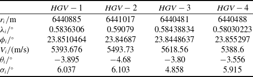
Scenario 1: Assume that no enemy threats are encountered during HGVs gliding, the leader HGV is designed to equilibrium gliding to increase the range, while ensuring that dynamic pressure, heating rate and normal overload are constrained.

The initial flight conditions are shown in Table 2:

The uncertainty caused by measurement errors is chosen as:

\begin{align*}\begin{array}{ll}\mathrm{\Delta }{\delta }_{\mathrm{2,1}} {} ={\left[\begin{array}{llllllllllllllllllll}3.1\times 1{0}^{-8}{\eta }_{\mathrm{2,11}}\quad {} 3.1\times 1{0}^{-7}{\eta }_{\mathrm{2,12}}\quad {} 3.1\times 1{0}^{-7}{\eta }_{\mathrm{2,13}} {} {} {} {} {} {} {} {} {} {} {} {} {} {} {} {} {} \end{array}\right]}^{T}\\[3pt] \mathrm{\Delta }{\delta }_{\mathrm{3,1}} {} ={\left[\begin{array}{llllllllllllllllllll}5\times 1{0}^{-8}{\eta }_{\mathrm{3,11}}\quad {} 5\times 1{0}^{-7}{\eta }_{\mathrm{3,12}}\quad {} 5\times 1{0}^{-7}{\eta }_{\mathrm{3,13}}\end{array}\right]}^{T}\\[3pt] \mathrm{\Delta }{\delta }_{\mathrm{4,1}} {} ={\left[\begin{array}{llllllllllllllllllll}1.27\times 1{0}^{-8}{\eta }_{\mathrm{4,11}}\quad {} 1.27\times 1{0}^{-7}{\eta }_{\mathrm{4,12}}\quad {} 1.27\times 1{0}^{-7}{\eta }_{\mathrm{4,13}}\end{array}\right]}^{T}\end{array}\end{align*}

The uncertainty in the aerodynamic coefficient is chosen as:

\begin{align*}\begin{array}{ll}\mathrm{\Delta }{\delta }_{\mathrm{2,2}} {} ={\left[\begin{array}{llllllllllllllllllll}2.5\times 1{0}^{-4}{\eta }_{\mathrm{2,21}}\quad {} 2.5\times 1{0}^{-5}{\eta }_{\mathrm{2,22}}\quad {} 2.5\times 1{0}^{-5}{\eta }_{\mathrm{2,23}} {} {} {} {} {} {} {} {} {} {} {} {} {} {} {} {} {} \end{array}\right]}^{T}\\[3pt] \mathrm{\Delta }{\delta }_{\mathrm{3,2}} {} ={\left[\begin{array}{llllllllllllllllllll}8.15\times 1{0}^{-4}{\eta }_{\mathrm{3,21}}\quad {} 8.15\times 1{0}^{-5}{\eta }_{\mathrm{3,22}}\quad {} 8.15\times 1{0}^{-5}{\eta }_{\mathrm{3,23}}\end{array}\right]}^{T}\\[3pt] \mathrm{\Delta }{\delta }_{\mathrm{4,2}} {} ={\left[\begin{array}{llllllllllllllllllll}1.27\times 1{0}^{-4}{\eta }_{\mathrm{4,21}}\quad {} 1.27\times 1{0}^{-5}{\eta }_{\mathrm{4,22}}\quad {} 1.27\times 1{0}^{-5}{\eta }_{\mathrm{4,23}}\end{array}\right]}^{T}\end{array}\end{align*}

The vehicle position measurement deviation at the initial moment is set as follows:

\begin{align*}\begin{array}{ll}{\zeta }_{\mathrm{2,1}}\left({t}_{0}\right) {} ={\left[\begin{array}{llllllllllllllllllll}5.4\mathrm{}\mathrm{m}\quad {} 1.3\times 1{0}^{-4}\mathrm{d}\mathrm{e}\mathrm{g}\quad {} -7.1\times 1{0}^{-5}\mathrm{d}\mathrm{e}\mathrm{g} {} {} {} {} {} {} {} {} {} {} {} {} {} {} {} {} {} \end{array}\right]}^{T}\\[3pt] {\zeta }_{\mathrm{3,1}}\left({t}_{0}\right) {} ={\left[\begin{array}{llllllllllllllllllll}-5.4\mathrm{}\mathrm{m}\quad {} 3.5\times 1{0}^{-5}\mathrm{d}\mathrm{e}\mathrm{g}\quad {} -1.2\times 1{0}^{-4}\mathrm{d}\mathrm{e}\mathrm{g}\end{array}\right]}^{T}\\[3pt] {\zeta }_{\mathrm{4,1}}\left({t}_{0}\right) {} ={\left[\begin{array}{llllllllllllllllllll}-10.9\mathrm{}\mathrm{m}\quad {} -6.75\times 1{0}^{-5}\mathrm{d}\mathrm{e}\mathrm{g}\quad {} 7.5\times 1{0}^{-5}\mathrm{d}\mathrm{e}\mathrm{g}\end{array}\right]}^{T}\end{array}\end{align*}

Select the external airflow disturbances as:

\begin{align*}\begin{array}{ll}\mathrm{\Delta }{\xi }_{\mathrm{2,1}}\left(t\right) {} ={\left[\begin{array}{llllllllllllllllllll}1.4+0.79\mathrm{}\mathrm{s}\mathrm{i}\mathrm{n}\frac{\pi }{20}t {} \left(2.785+1.58\mathrm{}\mathrm{s}\mathrm{i}\mathrm{n}\frac{\pi }{10}t\right)\times 1{0}^{-8} {} \left(2.785+1.58\mathrm{}\mathrm{s}\mathrm{i}\mathrm{n}\frac{\pi }{10}t\right)\times 1{0}^{-8} {} {} {} {} {} {} {} {} {} {} {} {} {} {} {} {} {} \end{array}\right]}^{T}\\[3pt] \mathrm{\Delta }{\xi }_{\mathrm{3,1}}\left(t\right) {} ={\left[\begin{array}{llllllllllllllllllll}0.71+3.96\mathrm{}\mathrm{s}\mathrm{i}\mathrm{n}\frac{\pi }{5}t {} \left(1.42+7.92\mathrm{}\mathrm{c}\mathrm{o}\mathrm{s}\frac{\pi }{20}t\right)\times 1{0}^{-8} {} \left(1.42+7.92\mathrm{}\mathrm{s}\mathrm{i}\mathrm{n}\frac{\pi }{10}t\right)\times 1{0}^{-8}\end{array}\right]}^{T}\\[3pt] \mathrm{\Delta }{\xi }_{\mathrm{4,1}}\left(t\right) {} ={\left[\begin{array}{llllllllllllllllllll}3.28+3.79\mathrm{}\mathrm{c}\mathrm{o}\mathrm{s}\frac{\pi }{10}t {} \left(6.56+7.58\mathrm{}\mathrm{s}\mathrm{i}\mathrm{n}\frac{\pi }{10}t\right)\times 1{0}^{-8} {} \left(6.56+7.58\mathrm{}\mathrm{c}\mathrm{o}\mathrm{s}\frac{\pi }{20}t\right)\times 1{0}^{-8}\end{array}\right]}^{T}\\[3pt] \mathrm{\Delta }{\xi }_{\mathrm{2,2}}\left(t\right) {} ={\left[\begin{array}{llllllllllllllllllll}0.27+0.24\mathrm{}\mathrm{s}\mathrm{i}\mathrm{n}\frac{\pi }{10}t {} \left(5.47+4.854\mathrm{}\mathrm{s}\mathrm{i}\mathrm{n}\frac{\pi }{5}t\right)\times 1{0}^{-5} {} \left(5.47+4.854\mathrm{}\mathrm{s}\mathrm{i}\mathrm{n}\frac{\pi }{20}t\right)\times 1{0}^{-5}\end{array}\right]}^{T}\\[3pt] \mathrm{\Delta }{\xi }_{\mathrm{3,2}}\left(t\right) {} ={\left[\begin{array}{llllllllllllllllllll}0.1265+0.48\mathrm{}\mathrm{c}\mathrm{o}\mathrm{s}\frac{\pi }{10}t {} \left(6.33+0.96\mathrm{}\mathrm{s}\mathrm{i}\mathrm{n}\frac{\pi }{20}t\right)\times 1{0}^{-5} {} \left(6.33+0.96\mathrm{}\mathrm{s}\mathrm{i}\mathrm{n}\frac{\pi }{10}t\right)\times 1{0}^{-5}\end{array}\right]}^{T}\\[3pt] \mathrm{\Delta }{\xi }_{\mathrm{4,2}}\left(t\right) {} ={\left[\begin{array}{llllllllllllllllllll}0.189+0.196\mathrm{}\mathrm{s}\mathrm{i}\mathrm{n}\frac{\pi }{10}t {} \left(3.79+3.92\mathrm{}\mathrm{c}\mathrm{o}\mathrm{s}\frac{\pi }{10}t\right)\times 1{0}^{-6} {} \left(3.79+3.92\mathrm{}\mathrm{s}\mathrm{i}\mathrm{n}\frac{\pi }{5}t\right)\times 1{0}^{-6}\end{array}\right]}^{T}\end{array}\end{align*}

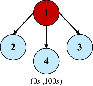
The design parameters of consensus controller are chosen as ${c}_{i,1}={[0.5,0.5,0.5]}^{T}$ , ${c}_{i,2}={[0.8,0.8,0.8]}^{T}$ , ${c}_{i,3}={[0.9,0.9,0.9]}^{T}$ . The filter parameters are selected as $ \tau =0.01$ . Consider the communication frequency to be $ 10\mathrm{}Hz$ , we set the simulation step as $ \mathrm{\Delta }t=0.01$ s. The communications topology graph used in the simulation is shown in Figure 5, where 1 represents the leader.

Table 3.

Initial conditions of the HGVs

Figure 5.

Communication topology for a leader and three followers.

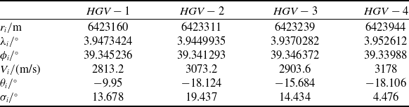
Scenario 2: Assume that spiral-diving manoeuver is adopted for the leader HGV to avoid interceptors and improve survival probability. Table 3 summarises the initial flight conditions.

Set the uncertainties, position measurement deviation, external airflow disturbances and communication topology same as Scenario 1. The design parameters of consensus controller are chosen as ${c}_{i,1}={[1,1,1]}^{T}$ , ${c}_{i,2}={[2.4,2.4,2.4]}^{T}$ , ${c}_{i,3}={[3.2,3.2,3.2]}^{T}$ . Figures 6 and 7 depict the flight state of the four HGVs.

Figure 6.

Formation flight trajectories of multi-HGV.

Figure 7.

Curves of $ {V}_{i}$ , $ {\theta }_{i}$ and $ {\sigma }_{i}$ along with time.

In scenario 1, the HGVs glide $ 20$ s in formation configuration to the north-east direction, whose velocity reduces to $ 5088.4$ m/s, flight path angle grow to $ -{1}^{\circ }$ , heading angle stabilise at $ 6.1{4}^{\circ }$ , altitude drop reposefully from $ 62.85$ km to $ 54.37$ km, with the ground track ending at $ \left(1.15{2}^{\circ }E,28.2{4}^{\circ }N\right)$ .

In scenario 2, the HGVs glide $ 100$ s in formation configuration to the north-east direction, performing two separate spiral-diving manoeuvers. The velocity of HGVs reduce to $ 1456$ m/s, flight path angle and heading angle fluctuate within $ [-7.{3}^{\circ },1.5{5}^{\circ }]$ sine and $ [7.{6}^{\circ },15.{1}^{\circ }]$ cosine, respectively; eventually the ground track ended at $ \left(4.43{8}^{\circ }E,41.14{7}^{\circ }N\right)$ .

Figures 8 – 10 show that in two scenarios, the formation configuration has basically been formed before $ t=14$ s and $ t=10$ s, respectively. In more detail, the longitudinal tracking errors $ {e}_{\mathrm{\Delta }{L}_{i}}$ of all followers are limited in 3 m, lateral tracking errors $ {e}_{\mathrm{\Delta }{W}_{i}}$ are limited in 5 m and vertical tracking errors $ {e}_{\mathrm{\Delta }{H}_{i}}$ are limited in 5 m. Furthermore, those errors no longer increase after the formation is formed, which can ensure the stability of the formation. This phenomenon demonstrates that no matter what initial flight conditions the follower HGVs have, no matter how the leader HGV glides, the proposed control method can achieve satisfactory results under the condition of uncertainty caused by measurement errors and external airflow disturbances.

Figure 8.

Longitudinal plane formation flight trajectories.

Figure 9.

Horizontal plane formation flight trajectories.

Figure 10.

Time histories of $ {e}_{\mathrm{\Delta }{L}_{i}}$ , $ {e}_{\mathrm{\Delta }{W}_{i}}$ and $ {e}_{\mathrm{\Delta }{H}_{i}}$ .

Figure 11 shows the deflection angle of speed brake $ {\delta }_{e,i}$ curve along with time of three follower HGVs, which is within a reasonable limit of $ [{0}^{\circ },4{0}^{\circ }]$ . Figure 12 shows the angle-of-attack $ {\alpha }_{i}$ curve along with time, which is within a reasonable limit of $ [-1{0}^{\circ },4{0}^{\circ }]$ . Figure 13 shows the bank angle $ {\upsilon }_{i}$ curve along with time, which is within a reasonable limit of $ [-9{0}^{\circ },9{0}^{\circ }]$ . These commands exhibit smoothness without high-frequency chatter and are consistent with practical engineering requirements. Moreover, the bank angle command to maintain stable formation flight does not exceed $ {5}^{\circ }$ . The simulation results demonstrate the effectiveness and potential application value of the designed control approach.

Figure 11.

The deflection angle of speed brake $ {\delta }_{e,i}$ curve along with time.

Figure 12.

The angle-of-attack $ {\alpha }_{i}$ curve along with time.

Figure 13.

The bank angle $ {\upsilon }_{i}$ curve along with time.

Figures 14 –19 displays the time histories of the estimated adaptive parameters $ \|{\widehat{\mathrm{\Theta }}}_{i}\|$ and the weight of network $ \|{\widehat{D}}_{i}\|$ . It is obvious that all signals are globally uniformly bounded.

Figure 14.

Time histories of $ \|{\widehat{\mathrm{\Theta }}}_{i,1}\|$ .

Figure 15.

Time histories of $ \|{\widehat{\mathrm{\Theta }}}_{i,2}\|$ .

Figure 16.

Time histories of $ \|{\widehat{\mathrm{\Theta }}}_{i,3}\|$ .

Figure 17.

Time histories of $ \|{\widehat{D}}_{i,1}\|$ .

Figure 18.

Time histories of $ \|{\widehat{D}}_{i,2}\|$ .

Figure 19.

Time histories of $ \|{\widehat{D}}_{i,3}\|$ .

4.2 Superiority verification

We use the same initial flight conditions and control parameters for all three methods. The consistent tacking errors of the three control methods are shown in Figure 20.

Figure 20.

Consistent tacking errors of three control methods.

Simulation results demonstrate that the proposed controller achieves a faster response during the initial formation tracking phase. When subjected to multisource disturbances and mismatched uncertainties, the MRAC-UAV method exhibits a significantly larger steady-state error, reaching 11 m, compared to the 8 m achieved by the proposed controller. Furthermore, the ANNC-UAV method shows slow convergence, with a convergence time of 12 s, and poor responsiveness, resulting in a transient tracking error of 25 m. In contrast, the proposed method converges in 10 s and maintains a consistent tracking error below 10 m after the system stabilises. These results clearly verify the effectiveness and advantages of the proposed adaptive distributed control method.