Introduction
The early stages of visual processing in striate cortex rely on multiple “channels” consisting of functionally-different neural units that operate like nonlinear filters. These “filters” each extract a narrow band of spatial frequency and orientation content from the retinal image (e.g., Campbell & Robson, Reference Campbell and Robson1968; Carandini et al., Reference Carandini, Demb, Mante, Tolhurst, Dan, Olshausen, Gallant and Rust2005; De Valois et al., Reference De Valois, Albrecht and Thorell1982a; De Valois et al., Reference De Valois, Yund and Hepler1982b; Graham & Nachmias, Reference Graham and Nachmias1971; Maffei & Fiorentini, Reference Maffei and Fiorentini1973; Merigan & Maunsell, Reference Merigan and Maunsell1993; Pantle & Sekuler, Reference Pantle and Sekuler1968; Phillips & Wilson, Reference Phillips and Wilson1984; Shapley & Lennie, Reference Shapley and Lennie1985; Ringach, Reference Ringach, Hawken and Shapley2002; Wilson & Bergen, Reference Wilson and Bergen1979). Simultaneous-masking studies have shown that the filters do not simply signal narrowband content in isolation but instead produce outputs that result from interactions between similarly, as well as differently, tuned filters, with those interactions leading either to suppression or facilitation of the detecting filter mechanism (e.g., Legge & Foley, Reference Legge and Foley1980; Morrone et al., Reference Morrone, Burr and Maffei1982; Olzak, Reference Olzak1985; Bonds, Reference Bonds1989; Bauman & Bonds, Reference Bauman and Bonds1991; Olzak & Thomas, Reference Olzak and Thomas1991; Ross & Speed, Reference Ross and Speed1991; DeAngelis et al., Reference DeAngelis, Robson, Ohzawa and Freeman1992; Polat & Sagi, Reference Polat and Sagi1993; Polat & Norcia, Reference Polat and Norcia1996; Bosking et al., Reference Bosking, Zhang, Schofield and Fitzpatrick1997; Fitzpatrick, Reference Fitzpatrick2000; Meier & Carandini, Reference Meier and Carandini2002; Yu et al., Reference Yu, Klein and Levi2002; Meese & Hess, Reference Meese and Hess2004; Petrov et al., Reference Petrov, Carandini and McKee2005; Meese & Holmes, Reference Meese and Holmes2007, Reference Meese and Holmes2010; Chen & Tyler, Reference Chen and Tyler2008; Huang & Hess, Reference Huang and Hess2008). Suppressive interactions between filters are thought to result from one of two distinct types of suppression, namely overlay suppression and surround suppression.Footnote 1 Further, neurophysiological studies have shown that the underlying neural processes involved in surround and overlay suppression stem from operations within two very different sites within the brain. Surround suppression is thought to originate within striate cortex as the suppression is narrowly tuned to the orientation and spatial frequency of the target and mask in both cat and nonhuman primate (DeAngelis et al., Reference DeAngelis, Robson, Ohzawa and Freeman1992, Reference DeAngelis, Freeman and Ohzawa1994; Fitzpatrick, Reference Fitzpatrick2000; Walker et al., Reference Walker, Ohzawa and Freeman2000; Akasaki et al., Reference Akasaki, Sato, Yoshimura, Ozeki and Shimegi2002; Cavanaugh et al., Reference Cavanaugh, Bair and Movshon2002; Osaki et al., Reference Osaki, Naito, Sadakane, Okamoto and Sato2011). Overlay suppression on the other hand is broadly tuned for both orientation and spatial frequency, and argued for this and other reasons to depend on LGN inputs to striate cortex (Bonin et al., Reference Bonin, Mante and Carandini2005; DeAngelis et al., Reference DeAngelis, Robson, Ohzawa and Freeman1992, Reference DeAngelis, Freeman and Ohzawa1994; Freeman et al., Reference Freeman, Durand, Kiper and Carandini2002; Li et al., Reference Li, Thompson, Duong, Peterson and Freeman2006; Morrone et al., Reference Morrone, Burr and Maffei1982; Priebe & Ferster, Reference Priebe and Ferster2006). In humans, Petrov et al. (Reference Petrov, Carandini and McKee2005) demonstrated psychophysically that overlay suppression is broadly tuned for orientation (∼180° full-width at half-height) and spatial frequency (∼3 octaves full-width at half-height), while surround suppression is narrowly tuned for orientation (∼30° full-width at half-height) and spatial frequency (∼1.4 octaves full-width at half-height). The broadly tuned nature of overlay suppression reported by Petrov et al. (Reference Petrov, Carandini and McKee2005) is consistent with the involvement of LGN-driven processes, as those inputs to V1 are generally not orientation selective. Similar claims of surround and overlay suppression have also been made by Meese and colleagues (Meese et al., Reference Meese, Challinor, Summers and Baker2009).
The overlay and surround suppression literature mentioned above has provided an important first step toward gaining insight into how the visual system operates with the complex input of every-day environments. However, that work has only investigated suppression as a result of narrowbandFootnote 2 targets and masks and can therefore only offer a simplified view of how different populations of filters may interact under conditions where more than a handful would be active. That is, the retinal image formed by real-world environments is known to be broadband in both spatial frequency and orientation (reviewed in Hansen et al., Reference Hansen, Haun, Essock, Portocello and Velloti2008), which means that at any given location within a scene, numerous visual filters are likely to be simultaneously active. Thus, the output of any given filter responding to real-world content will be weighted by the interdependent responses from a broad assortment of filters. Accordingly, recent advances in the simultaneous masking literature have focused on suppression generated by broadband masks. In particular, Essock and colleagues have shown that large broadbandFootnote 3 overlay masks (consisting of either visual noise or natural scene content) result in an elevation of contrast detection threshold that is highest for horizontal targets, intermediate for vertical, and lowest for oblique orientations; a suppressive phenomenon referred to as the “horizontal effect” (Essock et al., Reference Essock, DeFord, Hansen and Sinai2003; Hansen et al., Reference Hansen, Essock, Zheng and DeFord2003; Hansen & Essock, Reference Hansen and Essock2004, Reference Hansen and Essock2006; Essock et al., Reference Essock, Haun and Kim2009; Haun & Essock, Reference Haun and Essock2010). Further, this form of suppression has been shown to be narrowly tuned for orientation (∼40° full-width at half-height; Essock et al., Reference Essock, Haun and Kim2009; Hansen & Essock, Reference Hansen and Essock2006).
The horizontal effect has been typically measured at fixation with broadband stimuli of large spatial extent (typically subtending 4° of visual angle or more). As a result, the relative contribution of overlay and surround suppression is obscured, leaving open the possibility for either one (or both) as the primary suppressive mechanism underlying the effect (Essock et al., Reference Essock, Haun and Kim2009). However, given that the horizontal effect has been shown to involve suppression that is narrowly tuned for orientation, it would seem that surround suppression is the most likely mechanism. In an attempt to dissociate the relative roles of surround and overlay suppression in the horizontal effect (when tested at fixation), Kim et al (2010, Experiment 2.1) used temporally modulated Gabor targets (1° of visual angle) at one of four different orientations that were either embedded in, or surrounded by broadband noise (filtered to contain 15° orientation bandwidth and several octaves of spatial frequency content). The overlay mask conditions resulted in strong suppression overall and showed a prominent horizontal effect anisotropy (i.e., most suppression for horizontal targets embedded in horizontally filtered broadband noise, with lowest suppression observed for oblique targets and masks). Conversely, virtually no suppression was observed in the surround mask conditions (thereby precluding a measurable horizontal effect). The lack of any surround suppression for stimuli presented at the fovea is consistent with the findings of Petrov et al. (Reference Petrov, Carandini and McKee2005), who employed narrowband Gabor targets and masks at a single orientation (i.e., 45° oblique). Since the horizontal effect in the overlay condition at fixation is narrowly tuned for orientation, it seems unlikely that such narrowly tuned suppression would be dominated by broadly tuned subcortical (i.e., LGN) input, and suggests the involvement of an additional, second, source of overlay suppression that originates in cortex (Baker et al., Reference Baker, Meese and Summers2007; Kim et al., Reference Kim, Gheiratmand and Mullen2013; Kim, et al., Reference Kim, Haun and Essock2010; Meese & Baker, Reference Meese and Baker2009; Morrone et al., Reference Morrone, Burr and Maffei1982; Reference Morrone, Burr and Speed1987).
Given that broadband noise masks have been reported to result in tuned anisotropic overlay suppression, one question that stands out is whether that form of suppression is only measurable with overlay masks that are sufficiently broadband in spatial frequency. Traditional narrowband overlay suppression studies have only employed Gabor target stimuli and masks at a single test orientation. Therefore, the first major aim of the current study (i.e., Experiment 1) was to assess whether the overlay suppression anisotropy (i.e., the horizontal effect) at fixation can be observed with traditional Gabor targets and masks. To address this aim, Experiment 1 employed a psychophysical overlay suppression paradigm with traditional narrowband Gabor target stimuli embedded within narrowband Gabor masks presented at fixation. Broadband noise mask conditions were also included for reference. Finally, Experiment 1 also used narrowband and broadband surround masks in order to control for any accounts linked to surround suppression.
The second aim of the current study was to assess the underlying neural processes possibly involved in a cortical locus of overlay suppression that leads to a horizontal effect. Essock and colleagues (Essock et al., Reference Essock, DeFord, Hansen and Sinai2003; Hansen & Essock, Reference Hansen and Essock2004, Reference Hansen and Essock2006; Hansen et al., Reference Hansen, Essock, Zheng and DeFord2003) have suggested that the horizontal effect may operate via a divisive contrast gain control (or contrast normalization) process (e.g., Geisler & Albrecht, Reference Geisler and Albrecht1992; Heeger, Reference Heeger1992; Wilson & Humanski, Reference Wilson and Humanski1993; Carandini et al., Reference Carandini, Heeger and Movshon1997; Carandini & Heeger, Reference Carandini and Heeger2012) involving multiple “local” orientation-tuned gain pools (e.g., Schwartz & Simoncelli, Reference Schwartz and Simoncelli2001)—refer to the computational modeling section of the current study for further detail. Specifically, they proposed that within the orientation dimension, cortical suppression might be expected to be greater at certain orientation values due to the greater number of neurons tuned to those orientations. Crucial to that account, there is evidence in several species that there are fewer neurons in visual cortex tuned to oblique orientations than horizontal or vertical orientations (De Valois, et al., Reference De Valois, Yund and Hepler1982b; Kennedy et al., Reference Kennedy, Martin, Orban and Whitteridge1985; Maffei & Campbell, Reference Maffei and Campbell1970; Mansfield, Reference Mansfield1974; Mansfield & Ronner, Reference Mansfield and Ronner1978; Zemon et al., Reference Zemon, Gutowski and Horton1983). More recently, it has become apparent that there are also relatively more neurons tuned to horizontal than vertical (Mansfield, Reference Mansfield1974; Tiao & Blakemore, Reference Tiao and Blakemore1976; Mansfield & Ronner, Reference Mansfield and Ronner1978; Chapman et al., Reference Chapman, Stryker and Bonhoeffer1996; Chapman & Bonhoeffer, Reference Chapman and Bonhoeffer1998; Coppola et al., Reference Coppola, White, Fitzpatrick and Purves1998; Yu & Shou, Reference Yu and Shou2000; Li et al., Reference Li, Peterson and Freeman2003). Because of this numerical bias, the responses pooled in a local contrast normalization mechanism would be greatest for stimulus content near horizontal and least for content near oblique for stimuli which are equivalent other than in orientation (Essock et al., Reference Essock, DeFord, Hansen and Sinai2003; Hansen et al., Reference Hansen, Essock, Zheng and DeFord2003). Exactly how such a bias would operate in a cortical network has only been described generally with a single formal divisive operation (e.g., Hansen et al., Reference Hansen, Essock, Zheng and DeFord2003; Hansen & Essock, Reference Hansen and Essock2004). That is, a biophysically-inspired computational simulation of such a process has yet to be conducted. The second aim of the current study was therefore focused on building a functional model of cortical gain control that operates within a network of disproportionate populations of neurons tuned to different orientations and spatial frequencies. In doing so, it was our intent to examine whether such a model (with a fixed set of parameters) could simulate operations that may be linked to the suppression effects observed in Experiment 1.
While the first two focal points of the current study were designed to provide psychophysical data and computational insight regarding whether anisotropic overlay suppression requires broadband masks, they also lend further support to the notion of such suppression arising from cortical operations in human cortex. In order to provide a direct means of support for cortical involvement in humans, the third and final aim of the current study was to test whether anisotropic overlay suppression could be differentially modulated by transcranial direct-current stimulation (tDCS). Brain stimulation via tDCS is known to have its strongest influence at the cortical surface (e.g., Antal et al., Reference Antal, Nitsche and Paulus2001, Reference Antal, Nitsche and Paulus2006; Antal & Paulus, Reference Antal and Paulus2008; Nitsche et al., Reference Nitsche, Cohen, Wassermann, Priori, Lang, Antal, Paulus, Hummel, Boggio, Fregni and Pascual-Leone2008; Stagg et al., Reference Stagg, Best, Stephenson, O’Shea, Wylezinska, Kincses, Morris, Matthews and Johansen-Berg2009; Stagg & Nitsche, Reference Stagg and Nitsche2011). Thus, if the overlay suppression anisotropy has its origins in cortex, tDCS should be effective at modulating any observed anisotropic suppression effects (see the Introduction section of Experiment 2 for further details).
To summarize, the current study sought to (1) examine whether the overlay suppression anisotropy occurs only with broadband noise masks (Experiment 1), (2) assess whether such an anisotropic overlay suppression mechanism can be successfully simulated through a biophysically-inspired contrast gain control model that utilizes the numerical neuronal bias mentioned above, and (3) further test the notion that the overlay suppression anisotropy primarily arises from a cortical locus using tDCS (Experiment 2).
Experiment 1
Method
Apparatus
All stimuli were presented on a 21″ Viewsonic (G225fB) monitor driven by a dual core Intel® Xeon® processor (1.60 GHz x2) equipped with 4GB RAM, and a 256MB PCIe x16 ATI FireGL V7200 dual DVI/VGA graphics card with 8-bit grayscale resolution. The color management settings for the graphics card (i.e., 3D display settings) were adjusted such that the luminance “gain” of the green gun was twice that of the red gun, which was set to twice that of the blue gun. A bit-stealing algorithm (Tyler, Reference Tyler1997; Bex et al., Reference Bex, Mareschal and Dakin2007) was employed to yield 10.8 bits of luminance (i.e., grayscale) resolution (i.e., 1785 unique levels) distributed evenly across a 0–255 scale. Stimuli were displayed using a linearized look-up table, generated by calibrating with a Color-Vision Spyder3 Pro sensor. Maximum luminance output of the display monitor was 100 cd/m2 (50 cd/m2 mean luminance after calibration), the frame rate was set to 85 Hz, and the resolution was set to 1600 × 1200 pixels. Single pixels subtended 0.0134° of visual angle (i.e., 0.80 arc min.) as viewed from 1.0 m. Head position was maintained with an Applied Science Laboratories chin and forehead rest. Participants viewed the display monitor in a dark room through an aperture (16° of visual angle in diameter) of a large black circular mask that was fit to the monitor bezel in order to prevent any monitor or room orientation cues.
Participants
12 observers (7 female), 11 naïve to the purpose of the experiment, participated in the current experiment. The age of the participants ranged from 19 to 37 (modal age = 20). All participants had normal (or corrected to normal) vision and were screened by a series of vision tests to ensure that they had no acuity or astigmatism deficits. Finally, all participants gave institutional review board-approved written informed consent and were compensated for their time.
Stimulus construction
Target stimuli.
Three Gabor patterns (vertical, 45° oblique, and horizontal) were generated in the spatial domain (i.e., image pixel domain). The Gabors were generated by first creating a sinusoidal luminance profile (i.e., a sine wave grating) that was 8 cycles per degree (cpd) of visual angle when viewed from 1.0 m. We chose 8 cpd as the target's spatial frequency since previous reports (e.g., Haun & Essock, Reference Haun and Essock2010) have shown that target frequency to produce the largest horizontal effect. The grating was then windowed with a 2-D Gaussian (ramped to mean luminance) that allowed ∼2.0 periods of visible sinusoidal modulation (full-width at half-height). The result is a 1-octave (full-width at half-height) Gabor with ∼20° orientation bandwidth (full-width at half-height). The size of the targets (i.e., the Gaussian window at full-width and half-height) subtended 0.3° of visual angle at fixation. In order to reduce participant uncertainty regarding target location (Petrov et al., Reference Petrov, Carandini and McKee2005; Petrov et al., Reference Petrov, Verghese and McKee2006; Kim et al., Reference Kim, Haun and Essock2010), the target region was circumscribed with a low contrast circle (one pixel line thickness) that had a diameter of 0.38° of visual angle. For consistency, the circular location-cue was present in all conditions of the current study. Target contrast was controlled through a staircase algorithm (described in the Procedure section).
Narrowband overlay and surround masks.
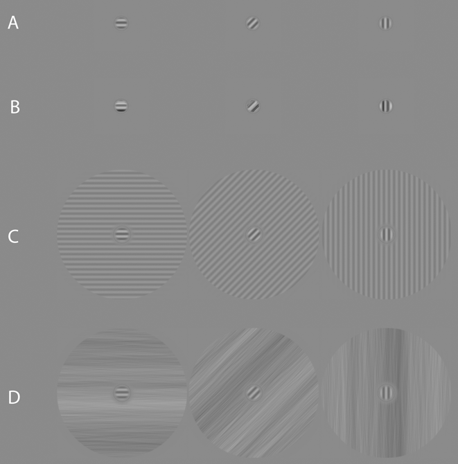
Three narrowband overlay and surround masks (vertical, 45° oblique, and horizontal) were constructed for this experiment. The overlay masks were created in an identical manner as the targets but were set to a fixed Michelson contrast of 30% (e.g., Petrov et al., Reference Petrov, Carandini and McKee2005), which corresponds to a root-mean-square (rms) contrast of 0.24. rms contrast was defined as the standard deviation of all pixel luminance values within a given image pattern, divided by the mean pixel luminance. The narrowband surround masks were generated in a similar manner as the targets. Once a sinusoidal grating had been created, it was windowed with two circular linear edge-ramps (ramped to mean luminance over 0.08°) so as to create an annulus that had an outer-edge diameter of 3.1° of visual angle, and an inner-edge diameter of 0.46° of visual angle, all at fixation. The surround masks were fixed at 10% Michelson contrast (e.g., Petrov et al., Reference Petrov, Carandini and McKee2005) which corresponds to an rms contrast of 0.08. Finally, the phase angle of the masks always matched that of the targets. Examples of the masks with targets present are shown in Fig. 1.
Example stimuli used in Experiment 1 (all showing target + mask). (a) Overlay masking condition: Gabor target superimposed on a Gabor mask of the same orientation and spatial frequency. (b) Overlay masking condition: Gabor target superimposed on a broadband noise patch possessing an orientation bandwidth of 20° (centered on the target's orientation) and a 2-octave bandwidth of spatial frequency (centered on the peak spatial frequency of the target). (c) Surround masking condition: Gabor target surrounded by a sinusoidal grating of the same orientation and spatial frequency. (d) Surround masking condition: Gabor target surrounded by a broadband noise pattern possessing an orientation bandwidth of 20° (centered on the target's orientation) and several octaves of spatial frequency content. The contrast of all examples has been scaled for visibility.

Broadband overlay and surround masks
The broadband masks consisted of visual noise with an amplitude spectrum fall-off of 1/f α. Noise masks were constructed in the Fourier domain using MATLAB (version R2012a) and generated uniquely on a trial-by-trial basis. Each mask was created by constructing a single 234 × 234 polar matrix for the amplitude spectrum, ISOAMP (f, θ), and assigning all coordinates the same arbitrary amplitude coefficient [except at the location of the direct current (DC) component which was assigned a zero]; f and θ represent spatial frequency and orientation, respectively. The result is a flat isotropic broadband spectrum. In this form, the exponent of the template spectrum could be adjusted by multiplying each spatial frequency's amplitude coefficient by ƒ−α, with α representing the exponent for the amplitude spectrum. For the current study, α was set to 1.0. The amplitude spectrum was then filtered with a triangle-wedge filter in orientation (see Kim et al., Reference Kim, Haun and Essock2010 for further details) with a peak value of 1.0 linearly ramped to zero across orientation. The orientation bandwidth of the filter was 20°. Once filtered, the amplitude spectrum can be considered fairly narrowband in orientation and broadband in spatial frequency.
The phase spectra [i.e., a different phase spectrum was used for mask type (overlay or surround) and for each trial] were constructed by assigning random values from −π to π to the different coordinates of a 234 × 234 polar matrix, Φ RAND (f, θ), such that the phase spectra were odd-symmetric—i.e., for θ angles in the [π, 2π] half of polar space, Φ RAND (f, θ) = Φ RAND (f, θ) × (−1).
The noise patterns were rendered in the spatial domain by taking the inverse Fourier transform of ISOAMP (f, θ) and a given Φ RAND (f, θ), with both shifted to Cartesian coordinates prior to the inverse DFT. Broadband overlay masks were sampled from the center of an orientation-filtered noise image (described above) to have the same spatial extent as the target (i.e., 0.3° of visual angle), and windowed with a circular edge-ramp (ramped to mean luminance). Note that the small size of the sampled noise used to create the overlay masks resulted in a 2-octave spatial frequency bandwidth (full-width at half-height) centered on the target's peak spatial frequency (the orientation bandwidth remained unchanged). Broadband surround masks were also created from a filtered noise image. The surround annulus was made in an identical manner as described for the narrowband surround masks. Lastly, the rms contrast of the overlay noise masks was fixed at 0.24, while the rms contrast of the surround noise masks was fixed at 0.08 (i.e., both were set to match the rms contrast of the narrowband masks). Examples of the masks with targets present are shown in Fig. 1.
Psychophysical procedure
The current experiment consisted of three target conditions and four mask conditions, grouped according to target orientation (vertical, 45° oblique, and horizontal), mask bandwidth (narrowband, broadband), and mask type (overlay, surround). An additional target only (i.e., no mask) condition was included in order to assess the strength of the masks on target detection relative to nonmasked detection. All masks were simultaneous with the target, with temporal onset and offset following a square wave function. Mask orientation always matched that of the target.Footnote 4 The stimulus presentation procedure consisted of a two-interval forced choice (2-IFC) paradigm, with the contrast of the targets controlled through a 2-down, 1-up staircase that approached threshold from above (target contrast step size was 0.05% Michelson contrast). For the broadband conditions, the same noise pattern was used for each 2-IFC interval of a given trial, with a different noise mask generated for each trial. Each staircase ran until 12 reversals were observed, with the average of the last 5 reversals serving as an estimate of detection threshold for a given staircase.
On any given trial, participants were first presented with a fixation dot (0.1°) at the center of the display screen for 300 ms. Participants were informed that the dot served to (1) signal that a stimulus interval would appear shortly, and (2) that the location of the dot would correspond to the location of the target stimulus. Following the fixation dot, two stimulus intervals were presented in succession (150 ms each), separated by a blank screen (set to mean luminance, 150 ms) followed by a second 300 ms fixation. Participants responded by keyboard as to which interval contained the target (the screen was blank during the response interval). The duration of the response interval was unlimited, and all viewing was binocular.
Each target orientation-by-mask type condition (including the no mask condition) was repeated six times, and blocked according to target orientation and mask type, for a total of 90 staircase blocks. All condition blocks were randomly interleaved. Before each block, participants were cued as to the orientation of the target they were trying to detect, as well as type of mask (or the lack thereof) within which the target would be embedded. The average time for each staircase block to reach 12 reversals was ∼3 min., for an average total experiment time of ∼4.5 h. Participants completed as many blocks as they could within 1-h long sessions that were run on separate days.
Results and discussion
The estimates of detection threshold for each condition were acquired by averaging the last four staircase thresholds that were gathered for each condition (i.e., the first two blocks for each condition were always treated as practice). Masked target thresholds were then converted to suppression factors by dividing the contrast detection threshold of the masked target by the contrast threshold of the target alone (e.g., Freeman et al., Reference Freeman, Durand, Kiper and Carandini2002; Kim et al., Reference Kim, Haun and Essock2010; Petrov et al., Reference Petrov, Carandini and McKee2005; Petrov et al., Reference Petrov, Verghese and McKee2006; Spiegel et al., Reference Spiegel, Hansen, Byblow and Thompson2012). Suppression factors above 1.0 indicate suppression. For each participant, a suppression factor was calculated for each condition for each of the last four thresholds and then averaged. Suppression factors for each target plus mask condition were generated by averaging suppression factors across participants.
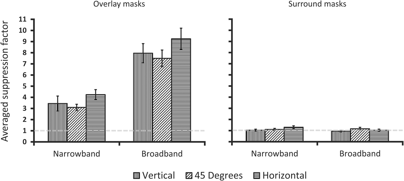
Group averaged suppression factors for each condition are plotted in Fig. 2. Interestingly, we found that the narrowband Gabor overlay mask conditions resulted in anisotropic suppression factors, with horizontal masks and targets yielding the highest suppression factors compared to 45° oblique.Footnote 5 As expected, the broadband mask conditions also produced anisotropic suppression factors. All overlay suppression factors differed significantly from 1.0 per one-sample t-tests (P < .001). Crucially, paired-samples t-tests show a statistically significant difference between horizontal and the 45° oblique condition for both narrowband masks (t 11 = 3.35, P < 0.01, d = 0.90) and broadband masks (t 11 = 2.28, P < 0.05, d = 0.60). The vertical suppression factor was intermediate to 45° oblique and horizontal and did not statistically differ from either (P > 0.05), which is consistent with the typical horizontal effect anisotropy (i.e., vertical being intermediate and not always statistically different from the other orientations). Finally, no suppression is apparent for either type of surround mask and there is no suppression anisotropy, which is consistent with previous reports using narrowband or broadband surround masks (e.g., Petrov et al., Reference Petrov, Carandini and McKee2005; Kim et al., Reference Kim, Haun and Essock2010). This observation was verified with the same statistical analyses described above which yielded no significant differences (P > 0.05).
Participant averaged data from overlay and surround mask conditions of Experiment 1. On the abscissa is the spatial frequency bandwidth of the masks, with the ordinate showing the averaged suppression factor [(target threshold with a mask)/(target threshold alone)]. Suppression factors above 1.0 indicate suppression of the target in the presence of a mask. Error bars are averaged within participant error and represent ±1 s.e.m.
Given the overlay suppression observed here, as well as the lack of any measurable suppression in the surround mask conditions, it does not appear as though a surround suppression mechanism can explain the horizontal effect anisotropy at fixation. This leaves overlay suppression operations as the most likely basis of the effect. Additionally, the spatial extent of the targets and masks in the overlay mask conditions further preclude any claims of surround suppression being involved in producing the horizontal effect at fixation. Since all target-mask orientations tested here were no more than 45° from one another, it seems highly unlikely that anisotropic overlay suppression reported in Fig. 2 is due to inputs from the LGN. Importantly, we find that within-target-channel suppression (i.e., the narrowband Gabor mask condition) can produce strong anisotropic suppression. That is, the overlay suppression anisotropy does not appear to require additional inputs from spatial frequency channels outside of those contained within the target (at least those at 8 cpd, where the horizontal effect has been reported to be at its strongest, i.e., Haun & Essock, Reference Haun and Essock2010). However, that is not to say that spatial frequency channels outside of the target do not play a role in the horizontal effect, just that such signals are not required to observe the effect.
Lastly, as noted in the general introduction, the horizontal effect observed with broadband masks has been explained in terms of contrast gain control that is differentially weighted by populations of neurons selective to different orientations (i.e., orientations that are processed by disproportionately more neurons result in larger reductions in signaling for those orientations). Therefore, the anisotropy reported here for both narrowband Gabor and broadband noise masks suggests that the differentially weighted contrast gain pool account can also be applied to more traditional overlay masking studies that employ Gabor stimuli. We explore this question in the following section.
Anisotropic contrast gain control simulation
The horizontal effect observed in suppression paradigms has been explained in terms of a contrast gain control process (i.e., divisive normalization), which is differentially weighted for stimulus orientation (Hansen et al., Reference Hansen, Essock, Zheng and DeFord2003; Hansen & Essock, Reference Hansen and Essock2004; Haun & Essock, Reference Haun and Essock2010; Kim et al., Reference Kim, Haun and Essock2010; Hansen & Hess, Reference Hansen and Hess2012). It has been demonstrated (Haun & Essock, Reference Haun and Essock2010) that threshold contrast for narrowband Gabor targets embedded within broadband noise can be well described by a modified contrast pattern masking model (Foley, Reference Foley1994), which varies gain modulation according to the orientation of the stimulus (target or mask). Such a model best fit the observer data when weights were greatest for horizontally oriented stimuli and weakest for oblique stimuli (Haun & Essock, Reference Haun and Essock2010). While such a psychophysical model of anisotropic gain modulation described the horizontal effect well, we thought it necessary to verify whether a biophysically-inspired population of neurons—with characteristics similar to those of simple cells in striate cortex and a numerical bias in preferred orientation—could generate anisotropic suppression signals within and/or across different spatial frequency channels that parallel the anisotropic contrast thresholds reported in Experiment 1. Accordingly, we designed a network of Integrate and Fire (I–F) neurons, which received as input the exact stimuli from Experiment 1, and verified if the proposed architecture of the horizontal effect could generate an anisotropic gain signal according to orientation of the target stimulus for both broadband and, more traditional, narrowband (Gabor) masking stimuli.
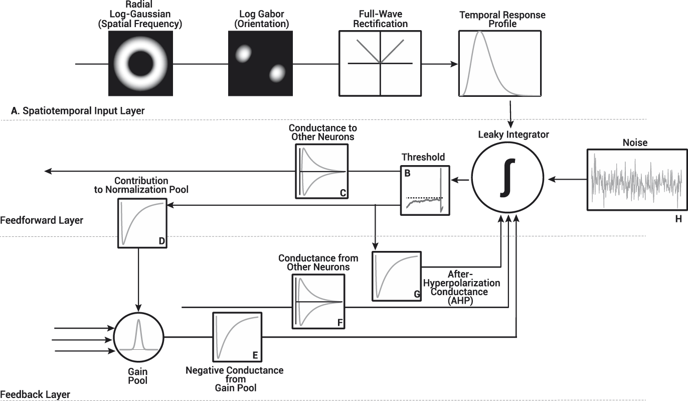
The network used for this simulation, shown in Fig. 3, is similar to that of previous simulations of neuron behavior in the primary visual cortex (Heeger, Reference Heeger1992; Carandini & Heeger, Reference Carandini and Heeger1994; Somers et al., Reference Somers, Nelson and Sur1995; Carandini & Ringach, Reference Carandini and Ringach1997; Carandini et al., Reference Carandini, Heeger and Movshon1997; Troyer et al., Reference Troyer, Krukowski, Priebe and Miller1998; Chance & Abbott, Reference Chance and Abbott2000; Pugh, Ringach, & Shapley, Reference Pugh, Ringach, Shapley and Shelley2000; Troyer et al., Reference Troyer, Krukowski and Miller2002; Ly & Doiron, Reference Ly and Doiron2009). The I–F neuron network contained a total of 2835 neurons (20% inhibitory), divided into three noninteracting spatial frequency channels (945 I–F neurons per channel; see Appendix A for more detail), each receiving input from spatial frequency filters centered either an octave below, on, or an octave above the spatial frequency of the Gabor targets used in Experiment 1. All I–F neurons received input from one of 12 oriented log-Gabor filters between 0° and 165° (in steps of 15°) as shown in Fig. 3A. We varied the number of I–F neurons tuned to a particular orientation within each spatial frequency group according to physiological findings reported by Li et al. (Reference Li, Peterson and Freeman2003). I–F neurons tuned to horizontal were most populous in the network (∼11% of preferred orientations) while 45° oblique tuned I–F neurons were least populous (∼6% of preferred orientations). This bias may however be different in humans (e.g., see Essock et al., Reference Essock, Haun and Kim2009).
Structure of the I–F neuron network used in our simulations. The operations within the network are divided into three layers: the spatiotemporal input layer transformed the stimuli from Experiment 1 into an input to drive the I–F neurons, while the I–F neuron themselves, were modeled as a combination of both feedback and feedforward operations. (A) The spatiotemporal input to the I–F neurons was modeled as a cyclical inner product in the Fourier domain with the radial profile of a log Gaussian, and the preferred orientation of the I–F neurons as a 2D Log-Gabor. The output of the Log-Gabor filters was full-wave rectified and subsequently convolved with the temporal profile of the spatiotemporal input. Each I–F neuron was modeled as a single voltage compartment, whereby the membrane potential of the i th I–F neuron, V i, was modeled as the summed input of: 1) a passive leak conductance, 2) voltage gated inputs from both the spatiotemporal input layer (A–Iinput) and synapses with other neurons (F–Isynapse), in addition to feedback loops used to normalize cell firing rate (G–IAHP and E–Igain) and, 3) Gaussian distributed noise used to mimic background activity (H–Inoise). (B) When the membrane potential of an I–F neuron reached its firing threshold (i.e., −54 mV), (C) the synaptic conductance it sent to the network (either excitatory or inhibitory), (G) the inhibitory conductance that contributed to the I–F neuron's self-inhibition and its (D) contribution to the gain pool were updated. All neurons within the network contributed and received inhibitory conductance (D, E) from the gain pool. The gain weights used to adjust the magnitude of the inhibitory conductance based on the preferred orientation difference of I–F neurons was defined as a Gaussian centered on 0 with a standard deviation of 15°. See Appendix A for further details.
Each neuron was modeled as a single voltage compartment, whereby the membrane potential of the ith I–F neuron, V i, was modeled as follows.
 $${\tau _i}{{d{V_i}} \over {dt}} = \left[ {\left( {{E_{{\rm{Leak}}}} - {V_i}} \right) - {I_{{\rm{input}}}} - {I_{{\rm{synapse}}}} - {I_{{\rm{AHP}}}} - {I_{{\rm{gain}}}} - {I_{{\rm{noise}}}} + {R_i}{I_{{\rm{ext}}}}} \right]\quad .$$
The present section focuses predominantly on a description of the normalization processes, mainly gain adjustments (I gain) implemented in the I–F neuron network, details on the input (I input), synaptic (I synapse), and self-recalibration (I AHP) currents used to define the membrane potential of our I–F neurons can be found in Appendix A.
There are two forms of normalization that serve to adjust the responses of cells. The first is a slow-acting self-recalibration mechanism (after hyper-polarization or AHP), while the second adjusts responses of cells based the pooled responses of a number of cells, i.e., gain control (Bonds, Reference Bonds1991; Heeger, Reference Heeger1992; Kohn, Reference Kohn2007). Self-recalibration in our I–F neurons was implemented as an after-hyperpolarization current (I AHP) with parameters designed to replicate the effects of a CA2+-gated K+ channels, as defined by Liu and Wang (Reference Liu and Wang2001); Sanchez-Vives et al. (Reference Sanchez-Vives, Nowak and McCormick2000a, Reference Sanchez-Vives, Nowak and McCormick2000b). This current increased according to the firing history of the I–F neuron, and slowed its firing rate (Ohzawa et al., Reference Ohzawa, Sclar and Freeman1985; Bonds, Reference Bonds1991; Sanchez-Vives et al., Reference Sanchez-Vives, Nowak and McCormick2000a, Reference Sanchez-Vives, Nowak and McCormick2000b; Dayan & Abbott, Reference Dayan, Abbott, Sejnowski and Poggio2005; Liu & Wang, Reference Liu and Wang2001). Gain control was implemented as an inhibitory current pooled from neighboring cells (i.e., within orientation channels) of the network. While gain-control is typically defined as a divisive operation in psychophysical models, in I–F neurons, it is defined as a change in the slope of the f–I curve, which relates the firing rate (f) to the driving current (I) of the I–F neuron (Holt & Koch, Reference Holt and Koch1997; Chance & Abbott, Reference Chance and Abbott2000; Chance et al., Reference Chance, Abbott and Reyes2002; Ly & Doiron, Reference Ly and Doiron2009). To obtain a change in the slope of the f–I curve, both an inhibitory current pooled from nearby I–F neurons (I gain) in Fig. 3E and current from background synaptic activity (I noise) in Fig. 3H must be added to the definition of the membrane potential of each neuron as shown in eqn. (1) (Holt & Koch, Reference Holt and Koch1997; Chance & Abbott, Reference Chance and Abbott2000). In isolation, the inhibitory current from the gain pool has only a subtractive effect on the firing rates of neurons, which will lead to a rightward shift in the f–I curve, without changing its slope. Conversely, background synaptic activity (I noise) raises firing rates at low driving currents, which leads both to a leftward shift and a change in the slope of the f–I curve (Holt & Koch, Reference Holt and Koch1997; Chance & Abbott, Reference Chance and Abbott2000; Ly & Doiron, Reference Ly and Doiron2009). When both are combined, the rightward shift generated by the inhibitory conductance from the gain pool and the leftward shift from background synaptic activity cancel, leaving only a change in the slope of the f–I curve, or a change in the gain of the I–F neuron. We modeled the current from background synaptic activity (I noise) as Gaussian distributed noise (ξ) with zero mean and standard deviation equal to 10% of the difference between the firing threshold (V threshold = −54 mV), and the reset potential of neurons (V reset = −80 mV), stated formally as follows.
 $${\sigma _{{\rm{noise}}}} = 0.1\left( {{V_\Theta } - {V_{{\rm{reset}}}}} \right)\quad ,$$
 $${I_{{\rm{noise}}}} = {\sigma _{{\rm{noise}}}}\xi \quad .$$
The current sent from the gain pool was defined as an inhibitory conductance that increased in magnitude over time according to the activity of neighboring neurons and weighted by the difference in their preferred orientation [see eqns. (5) and (6)], as defined by the following operation.
 $${I_{{\rm{gain}}}} = {r_i}{G_i}\left( {{V_i} - {E_{{\rm{gain}}}}} \right)\quad .$$
The reversal potential, E gain (−70 mV), was identical to that of the resting membrane potential, r i is the specific membrane resistance, and V i is the current membrane potential. The conductance from the gain pool was weighted according to the preferred orientation difference between I–F neurons within the network, formally expressed as follows.
 $${G_i} = \sum\limits_{j = 1}^N {{w_{{\rm{gai}}{{\rm{n}}_{ij}}}}{g_{{\rm{gai}}{{\rm{n}}_j}}}} \quad .$$
The gain adjustments were only defined for orientation preference and not spatial frequency. That is, I–F neurons in a given spatial frequency channel had no effect on the gain adjustments of other channels. Thus, gain adjustments were predominantly within-channel in orientation (Essock et al., Reference Essock, DeFord, Hansen and Sinai2003; Haun & Essock, Reference Haun and Essock2010; Kim et al., Reference Kim, Haun and Essock2010). The logic behind simulating noninteracting spatial frequency channels is primarily based on the fact that very little is known in terms of how different spatial frequency channels interact within a gain pool. For example, it is not clear whether their signals simply sum (e.g., Hansen & Hess, Reference Hansen and Hess2012), or whether they are differentially weighted (e.g., Haun & Essock, Reference Haun and Essock2010; Hansen & Hess, Reference Hansen and Hess2012; Haun & Peli, Reference Haun and Peli2013). It is customary to apply a flat (isotropic) gain pool to masking models (e.g., Watson & Solomon, Reference Watson and Solomon1997; Graham & Sutter, Reference Graham and Sutter2000) across orientation. Yet, when using natural scene stimuli there is evidence that weighted gain pools—which do not apply an even amount of inhibition across all stimulus dimensions—better fit both psychophysical data (Haun & Essock, Reference Haun and Essock2010; Haun & Peli, Reference Haun and Peli2013) and single neuron behavior (Schwartz & Simoncelli, Reference Schwartz and Simoncelli2001). Therefore, an anisotropic gain pool that pools more heavily from I–F neurons with similar preferred orientations has been argued to be better suited to characterizing the underlying mechanism of the horizontal effect (Hansen et al., Reference Hansen, Essock, Zheng and DeFord2003; Hansen & Essock, Reference Hansen and Essock2004), and we defined the gain pool scaling factor (w gain) as a Gaussian distribution centered on 0 (preferred orientation difference) and width equal to σ gain = 15°,
 $${w_{{\rm{gain}}}} = {{\rm{e}}^{ - \left( {{{{d^2}} \over {2{\sigma ^2}}}} \right)}}\quad ,$$
where d is the Euclidian distance between I–F neurons preferred orientation (see Appendix A). I–F neurons with identical orientation preference contributed heavily to each other's gain adjustments, while they had little impact on I–F neurons with different preferred orientations (see Fig. 4).
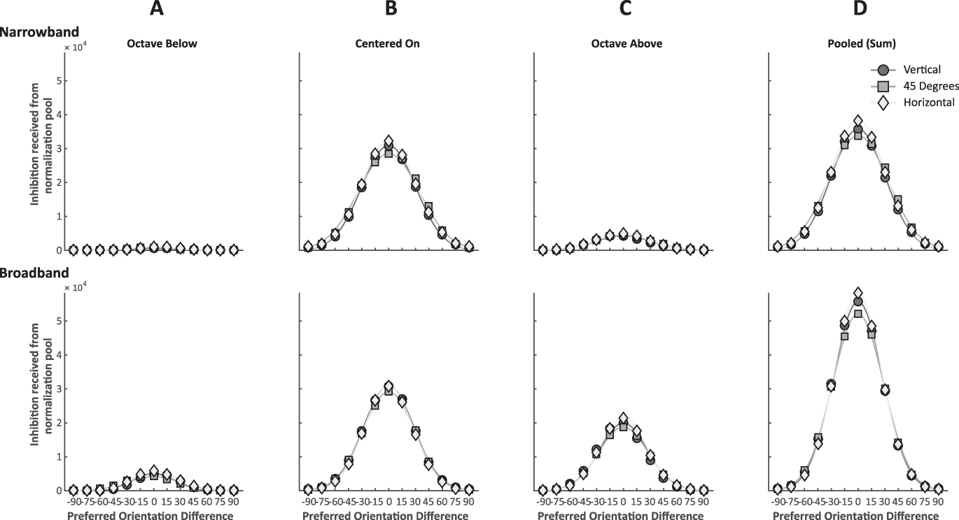
(A–C) Averaged total gain readjustment received for I–F neurons within the network following four 250 ms simulations with either a vertical (circles), oblique (squares) or horizontal (diamond) stimulus and mask. Each curve represents the gain received by a single I–F neuron given its preferred orientation difference with the stimulus and mask orientations. Points centered on the X-axis (0) therefore represent an I–F neuron with a preferred orientation identical to that of the stimulus and mask orientation. The gain readjustments were normally distributed and centered on the orientation of the stimulus. For all simulations, I–F neurons tuned to the orientation of the stimulus always received more gain readjustments than I–F neurons tuned to other orientations. The network shows the expected anisotropy for both narrowband Gabors and broadband noise masks, but only for I–F neuron's tuned to the orientation of the target. Horizontally tuned I–F neurons received more inhibition from the gain pool when the stimulus was horizontal than vertically or obliquely tuned I–F neurons when presented with a stimulus of their preferred orientation. In the narrowband Gabor mask condition, the anisotropy is only evident in I–F neurons with a preferred spatial frequency identical to that of the target stimulus. In the broadband noise mask condition, we find the expected anisotropy in all three spatial frequency channels. (D) Approximate gain readjustment when pooled (summed) across all three spatial frequency channels.
The gain pool conductance (g gain) was updated according to  ${g_{{\rm{gain}}}} \to {g_{{\rm{gain}}}} + \Delta {g_{{\rm{gain}}}}\left( {\Delta {g_{{\rm{gain}}}} = 3\,{\rm{ns}}} \right)$ when an I–F neuron within the network released an action potential, which built up in a series of steps increasing the inhibitory current conductance and leads the firing rate of I–F neurons to adapt. The conductance decreased to zero exponentially, with time constant τ gain (500 ms) when no action potentials were released within the network, as stated in eqn. (7).
 $${\tau _{{\rm{gain}}}}{{d{g_{{\rm{gain}}}}} \over {dt}} = - {g_{{\rm{gain}}}}\quad .$$
Simulations
In order to drive I–F neurons within our network, the stimuli (i.e., a target embedded in a mask) were first filtered and converted into a firing rate input response (I input) as shown in Fig. 3A (see Appendix A). Stimulus contrast was fixed for all simulations and stimulus conditions (target contrast was set to 5% Michelson contrast; mask contrast was set to 15% Michelson contrast). Each simulation was conducted in MATLAB (version R2014a) and used ODE45 to solve the differential equations used to simulate the I–F neuron network behavior for the first 250 ms following stimulus onset. Each simulation was repeated four times.
We verified whether a numerical bias in the preferred orientation of neurons could generate an anisotropic gain signal within each spatial frequency channel by collecting the total current sent from the gain pool for all I–F neurons throughout the simulations. Fig. 4A–4C shows the magnitude of the current received from the gain pool according to preferred orientation difference of I–F neurons, with each curve centered on the orientation of the target plus mask condition (vertical, 45° oblique or horizontal). As none of the spatial frequency groups interacted, the gain current received is shown for all three spatial frequency groups separately. The inhibitory conductance from the gain pool in the network has a similar anisotropy to the behavioral results of Experiment 1 for both narrowband and broadband masks. The magnitude of the gain signal is greatest when the target stimulus and mask orientation were horizontal and weakest when 45° oblique, while vertical lay between the two for both the narrowband Gabor and broadband noise mask conditions. Specifically, for I–F neurons centered on the spatial frequency of the target stimulus, the gain readjustment for the horizontal narrowband mask was 13% greater than that for 45° oblique narrowband mask and 4% greater than the vertical narrowband mask. The magnitude of the anisotropy in the centered on spatial frequency channel was less with the broadband mask in comparison to the narrowband mask, which can most likely be attributed to the slightly greater contrast energy of the Gabor mask (note that the contrast energy in the broadband mask is not symmetric about the center spatial frequency, i.e., it follows a 1/f α fall-off). Gain readjustments with a broadband mask showed an anisotropy (greater gain to horizontal masks) most clearly with I–F neurons tuned an octave above (41% greater than 45° oblique and 18% greater than vertical) and an octave below (15% greater than 45 oblique and 8% greater than vertical) the spatial frequency of the target stimulus, while I–F neurons centered on the target spatial frequency show the same magnitude of gain readjustment for both the vertical and horizontal masks, and a small difference (5%) between gain readjustments received between the horizontal and 45° oblique masks.
In order to provide a one-off approximation of what the gain readjustments would be after pooling, we took the linear sum of the gain readjustments across the three simulated spatial frequency channels for narrowband and broadband stimuli (Fig. 4D). As would be expected, the anisotropy is present in both, with narrowband targets and masks yielding horizontal readjustments 13% greater than 45° oblique and broadband targets and masks yielding horizontal readjustments 11% greater than 45° oblique.
The simulation results demonstrate that a small network of I–F neurons (with properties similar to those of simple cells within striate cortex), can generate an anisotropic gain signal that mirrors the anisotropy of contrast detection thresholds in the overlay masking paradigm of Experiment 1 for both narrowband Gabor and broadband noise masks. We show here that the theorized architecture of the horizontal effect can generate a gain anisotropy that is greatest for horizontally oriented stimuli and weakest for oblique stimuli. Further, our model simulations show that the anisotropy can be observed for within-spatial frequency channel processes operating on differently numerically biased populations of neurons. That is, the simulated anisotropic suppression does not require the activation of multiple spatial frequency channels as the narrowband stimuli do not possess a significant amount of contrast energy outside the target. Nevertheless, the anisotropy is still observable in the centered-on simulations. It is worth reiterating that these findings are not evidence for the horizontal effect suppression anisotropy to be primarily a within-spatial frequency channel process. Instead, we suggest that the anisotropy does not require pooled gain readjustments from across several spatial frequency channels.
Experiment 2
The behavioral results and functional model simulations presented in the current study, along with the findings reported previously by Kim et al (2010, Experiment 2.1), provide clear psychophysical and computational evidence in favor of overlay suppression having an orientation selective cortical component (in addition to the well-established non-orientation selective subcortical component mentioned earlier). While the evidence for cortical involvement in overlay suppression presented here is compelling on its own, it nevertheless is indirect evidence. The current experiment used tDCS to provide a direct test of whether early visual cortex plays a role in overlay suppression.
tDCS is a noninvasive brain stimulation technique that temporarily modulates the membrane potential of neurons in close proximity to stimulating electrodes placed on the scalp (Antal et al., Reference Antal, Nitsche and Paulus2001, Reference Antal, Nitsche and Paulus2006; Antal & Paulus, Reference Antal and Paulus2008; Nitsche et al., Reference Nitsche, Cohen, Wassermann, Priori, Lang, Antal, Paulus, Hummel, Boggio, Fregni and Pascual-Leone2008; Stagg et al., Reference Stagg, Best, Stephenson, O’Shea, Wylezinska, Kincses, Morris, Matthews and Johansen-Berg2009; Stagg & Nitsche, Reference Stagg and Nitsche2011). The technique involves a stimulating device that delivers a small DC between two head-mounted electrodes (anode and cathode), inducing an intra-cerebral electrical current flow from the anode electrode (current flowing into cortex) to the cathode electrode (current flow exiting cortex). Interestingly, studies of motor cortex tDCS have reported that the direction of current flow influences the effects of the stimulation. Specifically, anodal stimulation produces a “facilitative” effect on neural responses, whereas cathodal stimulation yields an “inhibitory” effect (Nitsche et al., Reference Nitsche, Fricke, Henschke, Schlitterlau, Liebetanz, Lang, Henning, Tergau and Paulus2003; Nitsche et al., Reference Nitsche, Doemkes, Karakose, Antal, Liebetanz, Lang, Tergau and Paulus2007; Nitsche & Paulus, Reference Nitsche and Paulus2000, Reference Nitsche and Paulus2011; Stagg et al., Reference Stagg, Best, Stephenson, O’Shea, Wylezinska, Kincses, Morris, Matthews and Johansen-Berg2009; Stagg & Nitsche, Reference Stagg and Nitsche2011). However, many factors including the cell type, cell morphology, and the direction of current in relation to the somatodendritic axis of pyramidal neurons influence the polarity specific effects of tDCS (Bikson & Rahman, Reference Bikson and Rahman2013; Radman et al., Reference Radman, Ramos, Brumberg and Bikson2009; Rahman et al., Reference Rahman, Reato, Arlotti, Gasca, Datta, Parra and Bikson2013; Reato et al., Reference Reato, Rahman, Bikson and Parra2010). As a result, it is perhaps not surprising that the evidence for polarity-specific effects of tDCS on visual cortical areas (e.g., primary visual cortex or area MT+) is less clear, in that only anodal or cathodal effects are observed, or effects that are opposite to those found over motor cortex are observed (e.g., Antal et al., Reference Antal, Nitsche and Paulus2001; Antal, Kincses, Nitsche, & Paulus, Reference Antal, Kincses, Nitsche, Bartfai and Paulus2004a, Reference Antal, Nitsche, Kruse, Kincses, Horrmann and Paulus2004b; Antal et al., Reference Antal, Kovács, Chaieb, Paulus and Greenlee2012; Jacobson, Koslowsky, & Lavidor, 2011; Kraft et al., Reference Kraft, Roehmel, Olma, Schmidt, Irlbacher and Brandt2010; Olma, Kraft, Roehmel, Irlbacher, & Brandt, Reference Olma, Kraft, Roehmel, Irlbacher and Brandt2011; Spiegel et al., Reference Spiegel, Hansen, Byblow and Thompson2012).
Conflicting polarity-specific influences of tDCS aside, the technique nevertheless offers the opportunity to test for the involvement of cortical processes related to behavioral performance as its effects are restricted to the cortical surface (e.g., Datta et al., Reference Datta, Bansal, Diaz, Patel, Reato and Bikson2009). We therefore reasoned that if the overlay suppression anisotropy has a cortical origin, tDCS should be effective at modulating anisotropic suppression effects.
The current study therefore set out to repeat the overlay conditions of Experiment 1 while participants received either anodal tDCS (a-tDCS) or cathodal tDCS (c-tDCS) stimulation (with stimulation performance compared to a non-stimulation baseline). The fact that a-tDCS or c-tDCS has been shown to produce differential effects on contrast detection performance (e.g., Antal et al., Reference Antal, Nitsche and Paulus2001; Kraft et al., Reference Kraft, Roehmel, Olma, Schmidt, Irlbacher and Brandt2010; Spiegel et al., Reference Spiegel, Hansen, Byblow and Thompson2012) allows for one form of stimulation to serve as a control for the other. Thus, any relative effects between either form and non-stimulation baseline serves as an indicator of cortical involvement in anisotropic overlay suppression. Taking such an approach allows us to side step confounds associated with sham stimulation as participants can usually detect when they are not being stimulated, yet cannot detect a difference between anodal vs. cathodal stimulation (e.g., Minhas et al., Reference Minhas, Datta and Bikson2011; Spiegel et al., Reference Spiegel, Hansen, Byblow and Thompson2012; Hansen et al., Reference Hansen, Andres, Essock, Spiegel and Thompson2013).
Materials and methods
Apparatus
The experimental display and computer, as well as the viewing conditions were to the same as those of Experiment 1. tDCS was generated using a 9V battery driven DC stimulator (Chattanooga Ionto, USA), and delivered via a pair of carbon-rubber electrodes (The Magstim Company Ltd., UK). The electrodes were encased in potassium chloride soaked Spontex sponge pockets (The Magstim Company Ltd., UK). The size of the stimulating electrode was 6 × 8 cm, and the size of the reference electrode was 12 × 8 cm, rendering the large reference electrode inert due to low current density (Nitsche et al., Reference Nitsche, Doemkes, Karakose, Antal, Liebetanz, Lang, Tergau and Paulus2007; Spiegel et al., Reference Spiegel, Hansen, Byblow and Thompson2012). Both electrodes were held in place with four rubber head-bands (The Magstim Company Ltd., UK), applied in a manner that ensured complete electrode sponge surface contact over the targeted scalp regions.
Participants
12 healthy observers were recruited for the current experiment. All participants were screened for previous or existing medical, neurological, or psychological conditions that could either put the participant at any undue risk, or interfere with stimulation efficacy (i.e., none of the participants were taking any type of psychotropic medication). All participants had normal (or corrected to normal) vision with no acuity or astigmatism deficits. All participants gave institutional review board-approved written informed consent and were compensated for their time. Of the 12 participants recruited for the current experiment, only 9 (6 female) had stable baseline thresholds that enabled them to participate in the tDCS sessions (see below for further details). The age of those participants ranged from 19 to 37 (modal age = 20), and 8 were naïve to the purpose of the experiment.
Target and mask stimuli
The same targets employed in Experiment 1 were also used in the current experiment (i.e., 8 cpd Gabor patches at three different orientations). The narrowband Gabor and broadband noise masks were constructed in an identical manner as in Experiment 1.
Psychophysical procedure
Practice conditions
In order to control for any practice effects that may confound tDCS effects, all participants in the current experiment repeated the conditions and procedure of Experiment 1, minus the surround mask conditions. Thus, the design of the practice conditions consisted of three target conditions and two mask conditions, grouped according to target orientation (vertical, 45° oblique, and horizontal) and mask bandwidth (narrowband, broadband). Target alone conditions were also included. All conditions were repeated 6 times (randomly interleaved), for a total of 54 staircase blocks. The average time to complete each staircase was again ∼3 min, for a total of ∼2.7 h total experiment time. Participants completed as many blocks as they could within 1-h long maximum sessions that were run on separate days. Participants who produced contrast detection thresholds that were stable (i.e., all within 1.5 standard deviations of one another) and showed no linear trends (increasing or decreasing) across the six repetitions were selected to proceed to the tDCS experimental conditions. The reason behind this screening procedure was to ensure that the tDCS participants yielded stable data that showed no signs of practice (or fatigue) effects. That is, the nonshunted DC that makes its way through to cortex is several orders of magnitude less than what is required to elicit action potentials (e.g., Creutzfeldt et al., Reference Creutzfeldt, Fromm and Kapp1962; Purpura & McMurty, Reference Purpura and McMurty1965; Tehovnik, Reference Tehovnik1996). The resulting modulation is therefore only at the membrane potential level, leading to increases (or decreases) in the probability of an action potential being elicited on the part of the visual stimulus. As a result, any expected influence of tDCS on behavior will be relatively small. Thus, in order to place the present experiment in an optimal position to detect any small changes in overlay suppression resulting from tDCS, we only included participants whose practice baselines were stable across the multiple repetitions of the practice sessions.
tDCS psychophysical conditions and stimulation procedure
The psychophysical procedure was identical to that used under the practice conditions. A single session of tDCS was limited to 30 min and therefore the number of repetitions for each condition (including the no mask condition) was restricted to two. The total number of staircase blocks in the tDCS sessions was therefore 18 [(3 orientations × 2 mask types × 2 repetitions) + (3 target only orientations × 2 repetitions)], with the condition order randomly interleaved. In order to ensure that participants would complete all staircases before the stimulation duration was finished, all staircases began closer to each participant's threshold than in the practice sessions. That is, once participants completed all practice blocks, the beginning contrast of the targets was set to two times each participant's practice threshold for each target + mask (and target alone) condition. All participants began each tDCS session (anode and cathode) by completing all 18 staircase blocks without tDCS stimulation. The results obtained from each session were averaged and used as the nonstimulation baseline. Immediately after the nonstimulation baseline conditions, participants repeated the 18 staircase blocks with tDCS stimulation. The tDCS sessions were conducted on separate days, with no less than 48 h separating the sessions. The order of the tDCS sessions (i.e., anode or cathode) was counterbalanced across participants. All participants completed the 18 staircase blocks during stimulation in under 30 min. Mean time to complete was 24.7 min, SD = 2.3 min.
The stimulating and reference electrode were positioned over Oz and Cz, respectively, in accordance with the 10–20 Electroencephalography (EEG) system. tDCS was delivered at 2 mA which yielded a current density of 0.042 mA/cm2 at the occipital electrode. The current was ramped up over an interval of 30 s. Participants waited 1 min once current stimulation reached its maximum before beginning the psychophysical task. Once each participant completed the 18 staircase blocks, the current was ramped down over the same 30 s interval. Once stimulation was complete, all participants were queried with a checklist regarding known minor poststimulation side effects (e.g., Nitsche et al., Reference Nitsche, Cohen, Wassermann, Priori, Lang, Antal, Paulus, Hummel, Boggio, Fregni and Pascual-Leone2008).
Results and discussion
There were no adverse effects of tDCS. Suppression factors for the pre-tDCS (i.e., nonstimulation), a-tDCS, and c-tDCS sessions were assembled in an identical manner as described in Experiment 1. Since there were two separate pre-tDCS data sets, we analyzed both in a 2 (pre-tDCS sessions) × 3 (target-mask orientation) two-way repeated measures analysis of variance (ANOVA). The main effect of session and the interaction were not statistically significant (P > 0.05). Thus, for the sake of simplicity, the suppression factors for each pre-tDCS session were averaged together to serve as a nonstimulation baseline.Footnote 6 The suppression factors obtained within the pre-tDCS sessions were all within 1.5 standard deviations of the averaged suppression factors measured during the practice sessions.
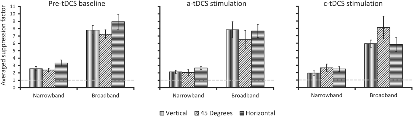
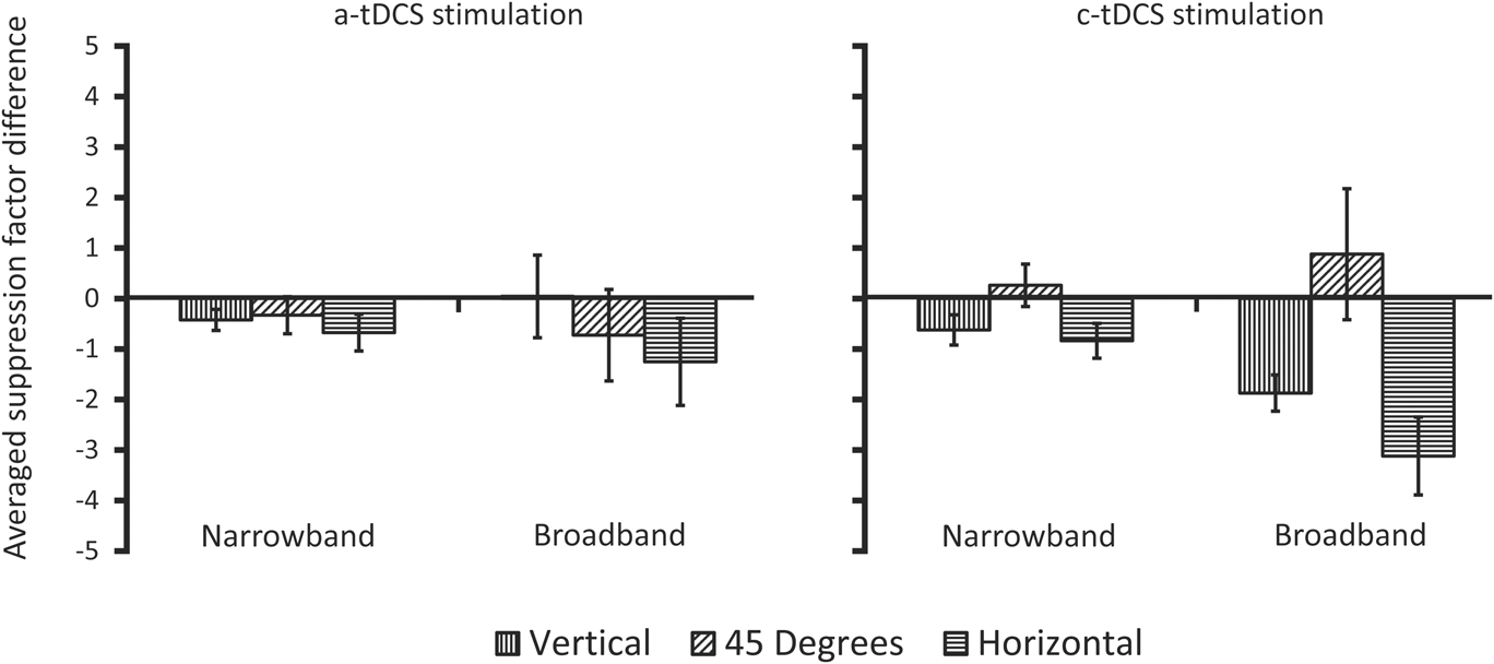
The averaged pre-tDCS suppression factors, along with those measured during a-tDCS and c-tDCS are plotted in Fig. 5. As an index of the influence of a-tDCS or c-tDCS on the suppression factors relative to the averaged pre-tDCS suppression factors, each participant's averaged pre-tDCS suppression factors were subtracted from their a-tDCS and c-tDCS suppression factors. These difference scores were then averaged across participants (Fig. 6). Negative values indicate a reduction in overlay suppression and positive values indicate an increase in overlay suppression.
Participant averaged overlay suppression data from Experiment 2. The abscissa and ordinate are identical to that shown in Fig. 2. Error bars are averaged within-participant error and represent ±1 s.e.m.
Re-plotted data from Fig. 5. Here, each participant's averaged pre-tDCS suppression factors have been subtracted from the suppression factors obtained under either a-tDCS or c-tDCS and then averaged. On the abscissa is the spatial frequency bandwidth of the mask condition, with the ordinate showing the across-participant averaged suppression factor differences (see text for further detail). Negative values indicate a reduction in overlay suppression, while positive values indicate an increase in overlay suppression. Error bars are averaged within-participant error and represent ±1 s.e.m.
One-sample t-tests showed all suppression factors reported in Fig. 5 to differ significantly from 1.0 (P < 0.01). For the averaged pre-tDCS condition, the horizontal effect anisotropy is again observed for both narrowband Gabor and broadband noise overlay masks. This observation was verified with planned comparison paired samples t-tests that revealed a statistically significant orientation anisotropy between horizontal and the 45° oblique condition for both broadband masks (t 8 = 2.46, P < 0.05, d = 0.82) and narrowband masks (t 8 = 2.97, P < 0.01, d = 0.98). Again, vertical was intermediate to 45° and horizontal, and did not significantly differ from either one (narrowband or broadband, P > 0.05). Interestingly, the influence of tDCS stimulation on the suppression factors is most apparent under cathodal stimulation for broadband masks, whereby the anisotropy virtually inverts, with increased suppression at 45° (albeit nonsignificant), and reduced suppression at vertical and horizontal. Anodal stimulation resulted in a small reduction in all suppression factors but also showed a slight anisotropic reduction in the broadband mask conditions (i.e., most reduction for horizontal, followed by 45°). These differences are best illustrated in Fig. 6, which shows the change in suppression factors for each stimulation condition relative to the no stimulation baseline. Concerning the differences in suppression factors between a-tDCS and pre-tDCS baseline, we ran two 2 (pre-tDCS, a-tDCS) × 3 (orientation) two-way repeated measures ANOVAs for each mask type (narrowband or broadband). For narrowband masks, both a-tDCS and c-tDCS produced a main effect of stimulation (a-tDCS: F 1,8 = 8.26, P <.05, partial η 2 = 0.50; c-tDCS: F 1,8 = 8.31, P <.05, partial η 2 = 0.51), and orientation (a-tDCS: F 2,16 = 9.75, P <.05, partial η 2 = 0.54; c-tDCS: F 2,16 = 4.55, P <.05, partial η 2 = 0.36). While there was no statistically significant interaction between stimulation (pre-tDCS, a-tDCS or c-tDCS) and orientation (P > 0.05), we did find a statistically significant difference between pre-tDCS and c-tDCS suppression factors for horizontally oriented narrowband masks (t 8 = 2.42, P < .05, d = 0.8). tDCS was ineffective at modulating masked target detection for 45°oblique targets, which is consistent with previous reports (e.g., Spiegel et al., Reference Spiegel, Hansen, Byblow and Thompson2012).
For broadband masks, only c-tDCS produced a main effect of stimulation (F 1,8 = 8.69, P <.05, partial η 2 = 0.52), and only a-tDCS showed a main effect of orientation (F 2,16 = 3.72, P <.05, partial η 2 = 0.32), with only c-tDCS showing a significant interaction between pre-tDCS and stimulation (F 2,16 = 4.76, P <.05, partial η 2 = 0.37). Regarding the significant main effect of stimulation (pre-tDCS vs c-tDCS), follow-up posthoc paired samples t-tests showed significant differences for broadband vertical and horizontal (t 8 = 5.2, P < .01, d = 1.74; t 8 = 4.9, P < .01, d = 1.34, respectively). Thus, we found tDCS to be most influential under cathode stimulation, with horizontal being significantly modulated when masked by either horizontal narrowband or broadband masks. Since we observed differential effects of a-tDCS vs c-tDCS stimulation (i.e., c-tDCS producing significant effects relative to pre-tDCS baseline), we can safely conclude that our results cannot be argued as a consequence of receiving mildly uncomfortable stimulation on the scalp.
General discussion
Previous studies have shown that when overlay masks that are narrowband in orientation and broadband in spatial frequency are used to mask narrowband Gabor targets at fixation, anisotropic overlay suppression is observed (e.g., Kim et al., Reference Kim, Haun and Essock2010), specifically a horizontal effect is observed (e.g., Essock et al., Reference Essock, DeFord, Hansen and Sinai2003). Such a finding would not be expected if overlay suppression primarily originates from initial LGN inputs to V1 (Petrov et al., Reference Petrov, Carandini and McKee2005) and implies that another, second, cortical operation is active at fixation when overlay masks are broadband in spatial frequency (Kim et al., Reference Kim, Haun and Essock2010). However, given that more traditional overlay masking studies that use only narrowband Gabor stimuli often only employ one target orientation, the question remained open as to whether a horizontal effect overlay suppression anisotropy is only apparent when numerous spatial frequency channels are active (i.e., when the overlay mask is broadband). That is, does the overlay mask have to contain more than one octave of spatial frequency content in order to observe the horizontal effect? Given the likely involvement of striate cortex in producing such a narrowly orientation-tuned suppression effect, it would seem that traditional Gabor masks should also yield suppression that varies across target-mask orientation. The results from Experiment 1 support this assumption as a horizontal effect overlay suppression anisotropy was observed at fixation for narrowband Gabor masks. Such a finding suggests that, at 8 cpd, a single spatial frequency channel's worth of content is sufficient to produce a suppression anisotropy. It is worth noting that previous studies using narrowband filtered noise masks have also argued for within-spatial-frequency channel gain operations being enough to produce the horizontal effect at detection threshold (Haun & Essock, Reference Haun and Essock2010) and in perceived contrast (Hansen & Essock, Reference Hansen and Essock2006). However, those studies used masks that subtended 4° of visual angle or more and therefore did not isolate overlay suppression operations.
In an attempt to provide a computational account of the overlay suppression anisotropy through cortical contrast gain control operations; our functional model verified that this form of overlay suppression can be reproduced through anisotropic gain control processes at the level of striate cortex.Footnote 7 Additionally, the functional gain control model simulated here consisted of a framework of well-known I–F neural network interactions that have been repeatedly implemented to simulate standard striate simple cell operations (Somers et al., Reference Somers, Nelson and Sur1995; Dayan & Abbott, Reference Dayan, Abbott, Sejnowski and Poggio2005). By simply adding a numerical bias to this network in terms of numbers of neurons tuned to different orientations, we observed responses by way of current received that would support anisotropic contrast gain control as a very likely mechanism underlying the additional second source of overlay suppression. Also, our model simulations produced anisotropic gain within the spatial frequency channel of the target for narrowband masks, and in all three channels simulated here for the broadband masks. Such a result provides computational support that the activation of multiple spatial frequency channels is not required to produce a behavioral overlay suppression anisotropy. It is important to note that while it is customary to emphasize broadly orientation-tuned suppressive interactions in masking models (Foley, Reference Foley1994; Watson & Solomon, Reference Watson and Solomon1997; Meese & Holmes, Reference Meese and Holmes2010), we chose to simulate narrow orientation-tuned suppressive interactions as this has been argued to be better suited to characterize the underlying mechanism of the horizontal effect (Hansen et al., Reference Hansen, Essock, Zheng and DeFord2003; Hansen & Essock, Reference Hansen and Essock2004). We did, however, verify the impact of an isotropic gain pool on the gain current received by I–F neurons in the network, while maintaining all other properties of the network identical, and found little difference between anisotropic (σ gain = 15°) and isotropic (σ gain = 90°) gain pools.
The results from Experiment 2 not only replicate the overlay suppression results observed in Experiment 1 (i.e., the pre-tDCS baseline condition) but also provide direct support for the likely involvement of cortex in producing anisotropic overlay suppression at fixation. Here, we find that c-tDCS was more influential at modulating anisotropic suppression when compared to pre-tDCS baseline and to the effects of a-tDCS. Further, we observed horizontal target + mask suppression to be significantly modulated by c-tDCS for both narrowband and broadband masks, thereby underscoring cortical involvement in the suppression anisotropy. Interestingly, c-tDCS resulted in larger modulation of the anisotropy produced by broadband masks than with narrowband masks. One likely explanation is that the broadband masks activated a greater number of spatial frequency channels (i.e., recruited more cortical activation), which in turn allowed c-tDCS to have a stronger modulatory effect.
Lastly, while tDCS is known to have polarity-specific effects in relation to the current direction (e.g., a-tDCS leading to increased likelihood of action potentials, with c-tDCS reducing action potential likelihood), such effects are not always observed when visual cortex is stimulated as discussed previously in Experiment 2 (c.f., Jacobson et al., 2011). The current study is no exception, as we found c-tDCS to be most influential in reducing anisotropic overlay suppression (i.e., target detection was improved most for horizontal targets). Ours, however, is not the only study to have found facilitatory effects of c-tDCS. When applied over the visual cortex, c-tDCS has been found to increase the amplitude of the P100 visual evoked potential (VEP) waveform both during stimulation and following stimulation (Accornero et al., Reference Accornero, Pietro, Riccia and Gregori2007; Antal et al., Reference Antal, Kincses, Nitsche, Bartfai and Paulus2004a). Similar effects of c-tDCS have also been found over other visually responsive cortical areas; c-tDCS over area MT improves motion discrimination in a dot kinetogram task when a coherent motion signal is presented amongst randomly moving dots (Antal et al., Reference Antal, Nitsche, Kruse, Kincses, Horrmann and Paulus2004b). As c-tDCS is believed to lead to an inhibitory modulation of neurons beneath the electrode, it may benefit performance in noise trials by decreasing the global activation and reduce the activation attributed to the noise below some threshold level. While the effects of tDCS when applied to the primary visual cortex may differ from those of area MT, the findings of Antal et al. (Reference Antal, Nitsche, Kruse, Kincses, Horrmann and Paulus2004b) could potentially explain how c-tDCS diminished the suppressive effects of the broadband masks. That is, c-tDCS may act to inhibit the larger lateral interactions of gain pool operations, thereby reducing their overall influence in the contrast normalization process and thus would have a reduced ability to suppress target detection.
To conclude, the current study provides further support for the existence of an additional form of overlay suppression (i.e., in addition to that taking place at the level of LGN-to-striate interactions) that originate in cortex, and extends what we know about this form of overlay suppression. Specifically, Experiment 1 demonstrated that narrowband Gabor masks (centered on 8 cpd) are sufficient to produce anisotropic overlay suppression at fixation, which can be modeled at the level of striate cortex through anisotropic gain control operating within spatial frequency channels. Together, Experiment 1 and our computational model suggest that the anisotropic operations resulting from a spatial frequency channel's worth of activation are sufficient to yield anisotropic overlay suppression, regardless of mask spatial frequency bandwidth (i.e., extensive cross-frequency pooling does not seem to be required to produce the effect, though it surely plays a role in driving the magnitude of the effect, e.g., Hansen & Essock, Reference Hansen and Essock2006). Lastly, c-tDCS was effective at modulating the overlay suppression anisotropy when the targets were superimposed on either narrowband or broadband masks, which provides direct support for the operations involved in the suppression anisotropy as having a cortical locus.
Acknowledgments
Portions of the current study were funded by the Colgate Research Council grant to BCH; BR was supported by a Fonds de Recherche du Quebec—Nature et Technologies (FRQNT) Doctoral Research Scholarship; a discovery grant from the Natural Sciences and Engineering Research Council (NSERC) of Canada to AJ.
Appendix A
The following describes the functional model used to simulate the anisotropic gain effects presented in text. The simulation can be subdivided into two main steps: the first converted stimuli from Experiment 1 into inputs used to stimulate the leaky I–F neurons in the second step of the simulation.
Spatiotemporal input
We modeled spatiotemporal input to I–F neurons as the cyclical inner product, in the Fourier domain, of our stimuli with the radial profile of a log Gaussian, and the preferred orientation of the I–F neurons as a 2D Log-Gabor. All filters employed were created using MATLAB (version 2013a) and referenced in polar coordinates. The input to the I–F neurons was calculated as the inner product in space and the convolution in time of our stimuli with the spatiotemporal weighting function of our Log-Gabors (G) defined as the product of spatial frequency selectivity [see eqn. (A2)] and orientation selectivity [see eqn. (A3)]. In symbols, it can be expressed as
 $$R\left( t \right) = \int\limits_0^T {\int\limits_{ - \infty }^\infty {\int\limits_{ - \infty }^\infty {G\left( {x,y} \right)T\left( t \right)} } } I\left( {x,y,\tau - t} \right)dxdyd\tau \quad .$$
The spatial frequency selectivity of our filters was defined as the radial profile of a log Gaussian
 $$D\left( \omega \right) = \exp \left\{ {{{ - \ln {{\left( {{\omega \mathord{\left/ {\vphantom {\omega {{\omega _0}}}} \right. \kern-\nulldelimiterspace} {{\omega _0}}}} \right)}^2}} \mathord{\left/ {\vphantom {{ - \ln {{\left( {{\omega \mathord{\left/ {\vphantom {\omega {{\omega _0}}}} \right. \kern-\nulldelimiterspace} {{\omega _0}}}} \right)}^2}} {2\left[ {\ln {{\left( {{k \mathord{\left/ {\vphantom {k {{\omega _0}}}} \right. \kern-\nulldelimiterspace} {{\omega _0}}}} \right)}^2}} \right]}}} \right. \kern-\nulldelimiterspace} {2\left[ {\ln {{\left( {{k \mathord{\left/ {\vphantom {k {{\omega _0}}}} \right. \kern-\nulldelimiterspace} {{\omega _0}}}} \right)}^2}} \right]}}} \right\}\quad ,$$
where ω 0 sets the center spatial frequency of the filter, which was set either to the center spatial frequency of the Gabor target (8 cpd), and octave above (16 cpd) or an octave below (4 cpd). The ratio k/ω 0 expresses the spatial frequency bandwidth of the filter full-width at half height (FWHH), which was set to one octave (k/ω 0 = 0.75).
The orientation arrangement of our filters was modeled as a bank of 2D log-Gabor filters (Field, Reference Field1987) in order to feed a signal selective in orientation to I–F neurons in a fashion roughly comparable to the pattern of geniculocortical connections in cat layer 4 (Reid & Alonso, Reference Reid and Alonso1995; Troyer et al., Reference Troyer, Krukowski, Priebe and Miller1998; Pugh et al., Reference Pugh, Ringach, Shapley and Shelley1999). The angular spread of a Log-Gabor, which controls their orientation sensitivity, was defined as a Gaussian centered on one of the 12 preferred orientations (from 0 to 165° in radians, θ) of our Log-Gabor filter bank.
 $$S\left( \theta \right) = \exp \left( {{{ - \theta _{{d_1}}^2} \mathord{\left/ {\vphantom {{ - \theta _{{d_1}}^2} {2\sigma _{{\theta _1}}^2}}} \right. \kern-\nulldelimiterspace} {2\sigma _{{\theta _1}}^2}}} \right) + \exp \left( {{{ - \theta _{{d_2}}^2} \mathord{\left/ {\vphantom {{ - \theta _{{d_2}}^2} {2\sigma _{{\theta _2}}^2}}} \right. \kern-\nulldelimiterspace} {2\sigma _{{\theta _2}}^2}}} \right)\quad .$$
The standard deviation of the spread function (σ θ = 0.35 θ), which sets its orientation bandwidth, used here was similar to that used by Somers et al. (Reference Somers, Nelson and Sur1995) and Carandini and Ringach (Reference Carandini and Ringach1997), and represents the relatively broad tuning of geniculocortical connections (Jones & Palmer, Reference Jones and Palmer1987; Reid & Alonso, Reference Reid and Alonso1995). The peak filter responses were normalized to equal 1 in order to have equivalent sensitivity across all orientations at the spatiotemporal layer of the model. The output of the Log-Gabor filters was full-wave rectified prior to being convolved with the temporal response profile of the spatiotemporal layer, defined as
 $$T\left( t \right) = \alpha \exp \left( { - \alpha t} \right)\left[ {{{{{\left( {\alpha t} \right)}^5}} \mathord{\left/ {\vphantom {{{{\left( {\alpha t} \right)}^5}} {5!}}} \right. \kern-\nulldelimiterspace} {5!}}} \right]\quad ,$$
a single phase version of the temporal response profile of a receptive field, as defined by Adelson & Bergen (Reference Adelson and Bergen1985), with α = 1/15 ms.
A Poisson process governed synaptic input from the spatiotemporal input to the I–F neurons, where k = 1/1000 (ms spikes)
 $$P\left( t \right) = R\left( \theta \right)k\Delta t\quad ,$$
with a mean rate, given the contrast of the stimulus (c), defined by eqn. A6 (R). S, which represents a baseline firing rate from the spatiotemporal input layer was set to 15.
 $$R\left( {\rm{c}} \right) = S + 25{\log _{10}}\left( {\rm{c}} \right)\quad .$$
Integrate-and-fire neurons
Excitatory and inhibitory I–F neurons were modeled separately using input resistances, membrane time constants and firing characteristics previously reported from both electrophysiological recordings and computational models (McCormick et al., Reference McCormick, Connors, Lighthall and Prince1985; Chu et al., Reference Chu, Milton and Cowan1994; Somers et al., Reference Somers, Nelson and Sur1995; Carandini & Ringach, Reference Carandini and Ringach1997; Troyer et al., Reference Troyer, Krukowski, Priebe and Miller1998; Dayan & Abbott, Reference Dayan, Abbott, Sejnowski and Poggio2005; Rudolph-Lilith et al., Reference Rudolph-Lilith, Dubois and Destexhe2009; Evans & Stringer, Reference Evans and Stringer2013). Each I–F neuron was modeled as a single voltage compartment for which the membrane potential for the ith neuron, V i, was given by eqn. (1), and accompanying parameters in Table A1. The membrane potential (V i) of an integrate-and-fire neuron was modeled as the summed input from a passive leak conductance (E leak − V i), voltage gated inputs from both the spatiotemporal input layer (I input) and synapses with other I–F neurons (I synapse), feedback loops used to normalize cell firing rate (I AHP and I gain) and a noise input used to mimic background activity (I noise). All input currents (I) to the I–F neuron, other than the noise input, were implemented as a spike-triggered linear conductance change with general form defined by eqn. (A7).
 $$I = {r_i}g\left( {{V_i} - E} \right)\quad .$$
Parameter list and values of Integrate-and-Fire neurons used in the anisotropic contrast gain control simulations
The conductance value (g) associated with each input current was updated according to  ${g_{e/i}} \to {g_{e/i}} + {\bar g_{e/i}}\left( {1 - {g_{e/i}}} \right)$ for excitatory and inhibitory synapses between I–F neurons and
 $g \to g + \Delta g$ for both fast (g AHP = 15 nS and Δg AHP = 6 nS) and slow (g gain = 15 nS and Δg gain = 3 nS) additive feedback operations. All conductance values decayed exponentially according to eqn. (A8) when no spike-triggered event occurred. The individual values for the time constant (τ), which defined the rate of decay, can be found in Table A1.
 $$\tau {{dg} \over {dt}} = - g\quad .$$
Firing threshold for both excitatory and inhibitory I–F neurons was set to −54 mV (V threshold). When the membrane potential of an I–F neurons reached V threshold, it was immediately brought to V reset = −80 mV, and maintained at that value for an absolute refractory period of the neuron, which was 3.6 ms for excitatory I–F neurons and 1.6 ms for inhibitory I–F neurons. I ext was set to 0 for all simulations.
Synaptic interactions (I synapse) between cortical I–F neurons were implemented as either AMPA-type excitatory synapses or GABAA-type inhibitory synapses (Somers et al., Reference Somers, Nelson and Sur1995; Carandini & Ringach, Reference Carandini and Ringach1997; Troyer et al., Reference Troyer, Krukowski, Priebe and Miller1998). No neuron synapsed with itself or received more than a single synapse from any I–F neuron in the network. In total, the model contained over 223,000 synapses across all three spatial frequency channels, of which, slightly more than half were excitatory. The probability of a synapse for excitatory and inhibitory I–F neurons was only defined for orientation preference and was chosen from a Gaussian distribution with a maximal synapse probability (p max) when the preferred orientation difference between two I–F neurons was 0 (Somers et al., Reference Somers, Nelson and Sur1995; Carandini & Ringach, Reference Carandini and Ringach1997), shown by eqn. (A9). The probability of an excitatory synapse between two I–F neurons with the same preferred orientation was set to 56.41 %, while it was 14.18% for inhibitory synapses. Excitatory synapses were drawn from a narrower range of preferred orientations (σ excit = 11.5°) than inhibitory synapses (σ inhib = 45°; Carandini & Ringach, Reference Carandini and Ringach1997; Evans & Stringer, Reference Evans and Stringer2013; Pugh et al., Reference Pugh, Ringach, Shapley and Shelley1999; Somers et al., Reference Somers, Nelson and Sur1995).
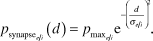 $${p_{{\rm{synaps}}{{\rm{e}}_{{e \mathord{\left/ {\vphantom {e i}} \right. \kern-\nulldelimiterspace} i}}}}}\left( d \right) = {p_{{{\max }_{{e \mathord{\left/ {\vphantom {e i}} \right. \kern-\nulldelimiterspace} i}}}}}{{\rm{e}}^{ - {{\left( {{d \over {{\sigma _{{e \mathord{\left/ {\vphantom {e i}} \right. \kern-\nulldelimiterspace} i}}}}}} \right)}^2}}}\quad .$$
The lateral connectivity matrix (d) was defined as the Euclidian distance between I–F neurons, based on their preferred orientation difference.
 $${d_{ij}} = \sqrt {\min {{\left( {\left| {{x_i} - {x_j}} \right|,\left| {\left| {{x_i} - {x_j}} \right| - {{\rm{S}}_x}} \right|} \right)}^2} + \min {{\left( {\left| {{y_i} - {y_j}} \right|,\left| {\left| {{y_i} - {y_j}} \right| - {{\rm{S}}_y}} \right|} \right)}^2}} \quad ,$$
where Sx and Sy refer to the size in the x and y dimensions of the population matrix. The min function implements a periodic boundary condition, making the one-dimensional matrix circular (Evans & Stringer, Reference Evans and Stringer2013). This pattern was implemented to generate a net lateral connectivity profile between inhibitory and excitatory I–F neurons that followed a “Mexican hat”—an effective approach to narrow the broad orientation input from the spatiotemporal layer (Somers et al., Reference Somers, Nelson and Sur1995; Carandini & Ringach, Reference Carandini and Ringach1997; Pugh et al., Reference Pugh, Ringach, Shapley and Shelley1999). The weighting factor of the gain pool, as described in text, was defined in an identical fashion to synapses between excitatory and inhibitory neurons, with parameter p max set to 1 and σ gain to 15°.