1. Introduction
Real-time kinematic (RTK) positioning is able to realise centimetre-level horizontal positioning accuracy ideally thanks to the differential technology and ambiguity resolution (Langley, Reference Langley1998; Teunissen, Reference Teunissen1995), which has been widely used in applications with high accuracy requirements, such as road transport (Teunissen, Reference Teunissen1995; El-Mowafy and Kubo, Reference El-Mowafy and Kubo2017). With the increasing number of available satellites, although the satellite geometry strength and redundancy of observations can be improved significantly, it cannot be ignored that the potential possibility of corrupted measurements is still increasing (Hewitson and Wang, Reference Hewitson and Wang2006; Joerger and Pervan, Reference Joerger and Pervan2016). Meanwhile, obstacles in complicated environments bring a great challenge to the normal reception of satellite signals (Zhu et al., Reference Zhu, Marais and Bétaille2018). The problems mentioned threaten the accuracy and reliability of RTK positioning solutions (Imparato et al., Reference Imparato, El-Mowafy and Rizos2018).
Fault detection and exclusion (FDE), as a means of quality control, is considered to guarantee the integrity of positioning solutions (Sun et al., Reference Sun, Wang and Cheng2021; Gao et al., Reference Gao, Jiang and Gao2021). According to hypothesis testing theory, FDE could detect and identify contaminated measurements, and further eliminate adverse impacts on positioning results. With the premise of a single fault of the positioning system due to limited GNSS constellations, typical FDE algorithms generally include the least squares residual method (Parkinson and Axelrad, Reference Parkinson and Axelrad1988), parity vector method (Sturza and Mark,Reference Sturza and Mark1988), maximum distance method (Grover Brown and McBurney, Reference Grover Brown and McBurney1988), etc. The least squares residual method and parity vector method are theoretically equivalent (Brown, Reference Brown1992) and both of them belong to FDE approaches in the range domain in which residuals are generally used to construct test statistics (El-Mowafy, Reference El-Mowafy2019). The maximum distance method is realised for the detection of a corrupted measurement in the position domain. Such approaches regard the estimator of the bias that would be introduced in the position solution by a significant anomaly in the observations as test statistics (El-Mowafy, Reference El-Mowafy2019). Due to increased visible signals from the global navigation satellite system (GNSS) and growing requirements on position performance from the users, these monitoring methods with the assumption of a single fault cannot be adapted in complicated scenarios, where observations experience multiple faults with high probability. For this, researchers extended conventional FDE methods. Considering the limitations, Hewitson and Wang (Reference Hewitson and Wang2006) proposed an extended w-test method for the identification of multiple outliers, which required the correlation information for test statistics and iterative re-evaluations of the test statistics after the exclusion of each outlier without the adjustment of observations. However, the calculation burden is not optimistic due to the growing number of faults. Zhang et al. (Reference Zhang, Zhao and Zhou2019) presented an improved method for single and multiple GNSS fault exclusion based on consensus voting and correlation analysis. However, the implementation process is relatively complex. Parkinson and Axelrad (Reference Parkinson and Axelrad1987) first introduced solution separation (SS), which was the baseline user algorithm in advanced receiver autonomous integrity monitoring (ARAIM) (Blanch et al., Reference Blanch, Walker and Enge2015). The separation between the full-set solution and the subset solution was used as a test statistic. Furthermore, multiple hypothesis solution separation (MHSS) as a type of SS algorithm is still accepted as a regular solution for solving multiple corrupted observations in the aviation domain (Blanch et al., Reference Blanch, Walter and Enge2010). However, from the point of view of the concept of separation, MHSS only focuses on the detection of faults that have a sensible impact on the position solution. Meanwhile, the foreknowledge about the number of faults, that is, all possible fault modes, is needed in these procedures, which is difficult in practical applications. In fact, the above research works are also essentially based on iteration and traversal algorithms. To overcome the dilemma, Yang and Xu (Reference Yang and Xu2016) developed a GNSS receiver autonomous integrity monitoring (RAIM) based on robust estimation. RAIM can not only detect multiple outliers, but also gauge the impact of near-contaminated measurements by experiments on GPS/Beidou data. Wang and Xu (Reference Wang and Xu2020) researched a modified residual-based RAIM algorithm based on robust MM estimation and the fast subset selection scheme.
Unfortunately, the above-mentioned approaches mainly consider the faulty pseudorange observations. Therefore, these methods could only be applied in metre-level positioning. However, the RTK technique features centimetre-level horizontal positioning accuracy ideally thanks to the ambiguity resolution based on carrier phase measurements. Recently, Wang and El-Mowafy (Reference Wang and El-Mowafy2021) analysed the effect of biases in integrity monitoring (IM) for RTK positioning, including designing a detailed threat model, which was able to distinguish between ambiguity-float and ambiguity-fixed scenarios, and using the SS method for the FDE procedure. Therefore, there still exist concerns about the calculation burden. There are two crucial bottleneck problems for fault detection and exclusion of RTK positioning: one is the development of an observation model that is suitable for faults monitoring, and the other is a reasonable and efficient fault detection and exclusion procedure.
Unreliable or erroneous ambiguity solutions, due to the impact of faulty observations and other disturbed errors, damage RTK positioning solutions in terms of accuracy and robustness. This paper proposes an improved FDE method based on a generalised least squares (GLS) model for RTK positioning. First, to provide a foundation for the observation model that is suitable for fault monitoring, the basic procedure of double-differencing (DD) integer ambiguity resolution is performed. Then, the GLS model, which is correlated due to the utilisation of differential technology (Liu et al., Reference Liu, Li and Zeng2019), is constructed by regarding fixed ambiguities passing the ratio test as the known parameters and putting them into the DD observation model. For rationality of fault detection and exclusion, data prewhitening is indispensable. Finally, the reliability of FDE results can be enhanced by the iterative reweighted least squares (IRLS) method rather than least squares (LS) without robustness. The main contributions are summarised as follows.
-
1. To develop a suitable observation model for fault monitoring, the generalised least squares DD model based on the fixed ambiguities is first constructed. Using the prewhitening procedure, an independent observation model is thus obtained, which provides a strong foundation for the introduction of classical fault detection methods only for a pseudorange.
-
2. Considering the importance of the residual components for rejecting abnormal observations, the ordinary LS estimator is replaced by the IRLS estimator. This improves the validity of residuals and thus the efficiency of the subsequent FDE method. Meanwhile, the traditional fault monitoring method is expanded into the carrier domain.
-
3. To verify the effectiveness of the proposed algorithm, a simulation and a real vehicular dynamic experiment are conducted. The results adequately indicate that the proposed method can provide high-precision and high-reliability RTK positioning solutions in the case of existing corrupted observation faults.
The rest of the paper is organised as follows. In Section 2, the basic theory about the contribution of DD observation equations and the GLS model is introduced. Then, model prewhitening and least squares estimation are presented in detail. Section 3 illustrates the improved FDE scheme combining the chi-square test with the w-test based on the iterative re-weighted least squares method. Section 4 analyses test statistics of the enhanced FDE algorithm and discusses the positioning performance between the proposed algorithm and the classical LS method in real experiments. Finally, several conclusions are provided in Section 5.
2. Background on observation model
In this section, the double-differencing observation model, as a typical model of RTK positioning, is first introduced. Then, the GLS model is constructed by putting fixed ambiguities into DD observation equations. Finally, the details of model prewhitening for uncorrelation and classical least squares estimation are presented.
2.1. Basic RTK positioning algorithm
Real-time kinematic positioning entirely removes most satellite-related errors, the receiver clock error and largely reduces atmospheric-related errors. The undifferenced uncombined observations concerning pseudorange and carrier phase can be denoted as follows (Gao et al., Reference Gao, Jiang and Gao2021):
 $$\left\{ {\matrix{ {\rho _{m,f}^i = P_m^i + c\left( {\delta {t_{{r_m}}} - \delta {t_{{s_i}}}} \right) - Vion_{m,f}^i - Vtrop_{m,f}^i + {\varepsilon _{\rho _{m,f}^i}}} \cr {{\lambda _f}\varphi _{m,f}^i = P_m^i + c\left( {\delta {t_{{r_m}}} - \delta {t_{{s_i}}}} \right) + Vion_{m,f}^i - Vtrop_{m,f}^i - {\lambda _f}N_{m,f}^i + {\varepsilon _{\varphi _{m,f}^i}}} \cr } } \right.$$
where
 $m$
denotes the receiver;
 $i$
is the order of visual satellite;
 $f$
represents frequency;
 $\rho $
and
 $\varphi $
denote pseudorange and carrier phase measurements for less than a circle, respectively;
 $\lambda $
is the carrier wavelength;
 $c$
is speed of light;
 $\delta {t_r}$
,
 $\delta {t_s}$
are receiver clock offset and satellite clock offset, respectively; the errors of ionosphere and troposphere are denoted by
 $Vion$
,
 $Vtrop$
, respectively;
 $N$
represents integer ambiguity in cycles;
 $\varepsilon $
is the noise of corresponding observations;
 $P_m^i$
denotes the geometric distance from receiver
 $m$
to satellite
 $i$
.
High-precision RTK positioning can be realised thanks to the utilisation of differential technology between stations and satellites. Double-differencing observation equations are summarised as follows:
 $$\left\{ {\matrix{ {\nabla \Delta \rho _{m,n,f}^{i,j} = \nabla \Delta P_{m,n}^{i,j} - \nabla \Delta Vion_{m,n,f}^{i,j} - \nabla \Delta Vtrop_{m,n,f}^{i,j} + {\varepsilon _{\rho _{m,n,f}^{i,j}}}} \cr {{\lambda _f}\nabla \Delta \varphi _{m,n,f}^{i,j} = \nabla \Delta P_{m,n}^{i,j} + \nabla \Delta Vion_{m,n,f}^{i,j} - \nabla \Delta Vtrop_{m,n,f}^{i,j} - {\lambda _f}\nabla \Delta N_{m,n,f}^{i,j} + {\varepsilon _{\varphi _{m,n,f}^{i,j}}}} \cr } } \right.$$
where
 $\nabla {\rm{\Delta }}$
is the double-differencing operator; the subscripts
 $m$
,
 $n$
,
 $f$
denote the operation between receiver
 $m$
and
 $n$
on the same frequency
 $f$
; the superscripts
 $i$
,
 $j$
are the reference satellite
 $i$
on frequency
 $f$
and satellite
 $j$
.
The errors from ionosphere and troposphere delay can be ignored when the distance between the basic station and rover station is short. Equation (2) can be simplified as
 $$\left\{ {\matrix{ {\nabla \Delta \rho _{m,n,f}^{i,j} = \nabla \Delta P_{m,n}^{i,j} + {\varepsilon _{\rho _{m,n,f}^{i,j}}}} \cr {{\lambda _f}\nabla \Delta \varphi _{m,n,f}^{i,j} = \nabla \Delta P_{m,n}^{i,j} - {\lambda _f}\nabla \Delta N_{m,n,f}^{i,j} + {\varepsilon _{\varphi _{m,n,f}^{i,j}}}} \cr } } \right.$$
Based on a first-order Taylor series expansion, a linearised observation model about user position and ambiguity parameters is expressed as follows:
 $${\rm{l}} - {{\rm{l}}_0} = {\bf{H}} \times \left( {{\rm{X}} - {{\rm{X}}_0}} \right)$$
where
 ${{\bf{X}}_0}$
is the initialisation state;
 $l$
is the observation vector;
 ${\bf{H}}$
is the design matrix;
 ${{\rm{l}}_0}$
depends on the selection of initialisation state
 ${{\bf{X}}_0}$
.
Aimed at the model given by Equation (4), ambiguity resolution is a crucial step for the centimetre-level positioning accuracy of RTK. According to the regular resolution procedure, the high precision can be fulfilled by putting the fixed ambiguities passing ratio test into the classical DD observation model. However, the process of solving fixed ambiguities is inevitably to be disturbed by multiple factors due to the inherent vulnerability of GNSS signals and the complexity of the surrounding environment. Therefore, the correctness of fixed integer ambiguities is vital for the accuracy and robustness of positioning.
2.2. Generalised least squares model
The generalised least squares model is formed by substituting the fixed ambiguities as known parameters back into the linearised model expressed by Equation (4),
 $${{\rm l}_k} = {{\rm A}_k}{{\rm x}_k} + {{\rm v}_k}$$
where the estimated state
 ${{\rm x}_k}$
is only related to the position;
 $\rm l$
is the
 $d$
-dimension observation vector; the covariance matrix of observation noise
 ${{\bf{v}}_k}$
is
 ${{\rm{C}}_{{{\rm l}_k}}}$
with properties of symmetry and positive definite. The generalised least squares model is a popular linear model. Compared with the ordinary least squares (OLS), it cannot require independence between observations (Menke, Reference Menke2015).
According to the construction of the DD observation model, the covariance matrix of observation noise is off-diagonal due to the correlation of DD measurements (Liu et al., Reference Liu, Li and Zeng2019). However, it is averse to designing an efficient fault detection and exclusion procedure reasonably. The classical FDE method for pseudorange usually holds the assumption that the observations are independent of each other and even follow the same normal distribution. With this background, the integrity requirement (probability of false alarm) is equally allocated to each observation and the construction of crucial test statistics is relatively easy thanks to the good statistical independence property for normal distribution. The problems induced by correlated measurements therefore can be summarised as two main points in detail. One is that the integrity requirements cannot be allocated equally to every observation denoted as
 $l$
. The other is that for the global faults test, the freedom of degree parameter, which is important for the calculation of the detection threshold, is difficult to determine in contrast to the traditional method. Therefore, it is desirable for decorrelation data in the linear regression.
The prewhitening method has been accepted as a normal decorrelation process in control and communication fields (Gandhi and Mili, Reference Gandhi and Mili2010). Based on the unique property of the noise covariance matrix, the core step of prewhitening is the Mahalanobis transformation (Wu et al., Reference Wu, Jia, Johansson and Shi2013). The prewhitening factor
 ${\rm L}_k^{ - 1}$
meets the following equation, that is,
 ${{\bf{C}}_{{{\rm l}_k}}} = {{\bf{L}}_k}{\bf{L}}_k^T$
. Specifically, a prewhitening operation is performed on the linearised model expressed as
 $${\bf{L}}_k^{ - 1}{{\bf{l}}_k} = {\bf{L}}_k^{ - 1}{{\bf{A}}_k}{{\rm x}_k} + {\bf{L}}_k^{ - 1}{{\bf{v}}_k}$$
For convenience, it is further expressed as follows:
 $${\bf{l}}_k^{\rm{*}} = {\bf{A}}_k^{\rm{\ast}}{{\bf{x}}_k} + {\bf{v}}_k^{\rm{\ast}}$$
The prewhitened noise
 ${\bf{v}}_k^{\rm{*}}$
follows the standard Gaussian distribution in
 $d$
-dimension, where
 $d$
denotes the number of measurements.
According to least squares estimation, the estimated state and corresponding covariance are
 $$\left\{ {\matrix{ {{{{\bf{\hat x}}}_{\rm{k}}} = {{\left( {{\bf{A}}{{_k^{\rm{*}}}^T}{\bf{A}}_k^{\rm{*}}} \right)}^{ - 1}}{\bf{A}}{{_k^{\rm{*}}}^T}{\bf{l}}_k^{\rm{*}}} \cr {{{\bf{Q}}_{{{{\rm{\hat x}}}_k}}} = {{\left( {{\bf{A}}{{_k^{\rm{*}}}^T}{\bf{A}}_k^{\rm{*}}} \right)}^{ - 1}}} \cr } } \right.$$
Based on estimated states, the residual vector and the corresponding covariance matrix can be calculated as
 $$\left\{ {\matrix{ {{{\bf{V}}_k} = {\bf{l}}_k^{\rm{*}} - {\bf{A}}_k^{\rm{*}}{{{\bf{\hat x}}}_k}} \cr {{{\bf{Q}}_{{{\bf{V}}_k}}} = {{\bf{I}}_m} - {\bf{A}}_k^{\rm{*}}{{\left( {{\bf{A}}{{_k^{\rm{*}}}^T}{\bf{A}}_k^{\rm{*}}} \right)}^{ - 1}}{\bf{A}}{{_k^{\rm{*}}}^T}} \cr } } \right.$$
Residuals, as crucial components of construction of faults test statistics, are related to LS estimated states. In other word, the statistics are the function of parameter estimation. However, the classical LS method is not robust to the outliers, resulting in the phenomenon of missed detection or false detection.
3. Improved fault detection and exclusion method
In this section, the iterative re-weighted least squares method is first presented in detail. Then, an improved FDE scheme combining the chi-square test with the w-test is introduced, which is based on the theory of hypothesis testing. Finally, the core steps of the proposed method are summarised in a table.
3.1. Iterative re-weighted least squares
The estimation results based on classical LS could be seriously impacted by corrupted measurements, even divergence. There are several benefits for fault detection and exclusion results enhanced by robust estimation. One is the guarantee of reliability of FDE results. The other is further enhancement of fault-tolerance ability of the whole positioning system. For more reliable test statistics, the iterative re-weighted least squares method is adapted in this paper due to its unique robustness and simplification.
According to the maximum likelihood estimate (MLE) theory (Knight and Wang, Reference Knight and Wang2009; Crespillo et al., Reference Crespillo, Andreetti and Grosch2020), the objective function of M estimation is expressed as follows:
 $${{\bf \hat x}_M} = {\rm{arg}}\mathop {{\rm{min}}}\limits_x \sum\limits_{i = 1}^d \kappa \left( {{{{V_i}\left( x \right)} \over {{\sigma _{{V_i}}}}}} \right)$$
where
 $\kappa \left( \cdot \right)$
is the cost function whose input variable is normalised residuals;
 ${V_i}$
is the ith element of residual vector;
 ${\sigma _{{V_i}}}$
denotes the standard deviation of the residual;
 $d$
represents the total number of observations.
As shown in Equation (10), parameter estimation belongs to the optimisation problem. Based on optimisation theory, the optimisation problem can be solved as
 $${{\bf \hat x}_M} = {\rm{arg}}\mathop {{\rm{min}}}\limits_x \mathop \sum \limits_{i = 1}^d w\left( {{\upsilon _i}} \right)\upsilon _i^2$$
where
 $w\left( {} \right)$
is the equivalent weight function that is related to the derivative of the cost function;
 ${\upsilon _i}$
denotes normalised residuals.
According to the principle of Gaussian efficiency, the robust standardised residuals can be calculated as follows:
 $${\upsilon _i} = {{{V_i}} \over {1.4826 \times med\left( {\left| {{V_i} - \mathop {med}\limits_i \left( {{V_i}} \right)} \right|} \right)}}$$
where the constant
 $1.4826$
represents a correction factor for Fisher consistency at the Gaussian distribution (Gandhi and Mili, Reference Gandhi and Mili2010);
 $med\left( \cdot \right)$
is the median operation.
Appropriate equivalent weight functions are designed to make the weights of outliers as small as possible. Huber, Tukey and IGG (Wang and Xu, Reference Wang and Xu2020) are the common equivalent weight functions. The Huber score function is selected in this paper and the weight elements from Equation (11) are computed as follows:
 $$w\left( {{\upsilon _i}} \right) = \left\{ {\matrix{1 \,\,\,\,\,\,\, {\left| {{\upsilon _i}} \right| \lt {k_H}} \cr \!\!\!\!\!\!\!\!\!\!\!\!{{{{k_H}} \over {\left| {{\upsilon _i}} \right|}}} \,\,\,\,\,\,\,{{\rm{else}}} \cr } } \right.$$
where
 ${k_H}$
denotes the robust coefficients, which are used to determine whether an observation is valid or not (Jiang et al., Reference Jiang, Pan and Meng2022). In general, the value of
 ${k_H}$
is equal to
 $1.5$
for
 $95{\rm{\% }}$
Gaussian asymptotic efficiency.
The state correction at the jth iteration is calculated by (Gandhi and Mili, Reference Gandhi and Mili2010; Crespillo et al., Reference Crespillo, Medina and Skaloud2018)
 $${{\bf{\hat x}}^{\left( {j + 1} \right)}} = {\left( {{\bf{A}}_k^{{\rm{*}}T}{{\bf{W}}^{\left( j \right)}}{\bf{A}}_k^{\rm{*}}} \right)^{ - 1}}{\bf{A}}_k^{{\rm{*}}T}{{\rm{W}}^{\left( j \right)}}{\bf{l}}_k^{\rm{*}}$$
where the weight matrix
 $W$
is diagonal. The algorithm converges when
 $\vert\vert{{\bf{\hat x}}^{\left( {j + 1} \right)}} - {{\bf{\hat x}}^{\left( j \right)}}_2 \vert\vert\le tol$
, where
 $tol$
is the tolerance factor. It is equal to
 $0.01$
in this paper. It shows that in experiments, the algorithm can generally converge within two iterations with enough observations and within five iterations at each time step in slightly worse observation environments.
3.2. Improved fault detection and exclusion method
The residual-based fault detection and exclusion scheme depends on the theory of hypothesis testing. The key steps include the calculation of critical thresholds and the construction of test statistics. Combined with the theory of binary hypothesis tests, the faults will be identified and excluded in the positioning system.
The global fault detection statistic
 ${s_k}$
is (Parkinson and Axelrad, Reference Parkinson and Axelrad1988)
 $${s_k} = \sqrt {{{SSE} \over {\left( {d - 3} \right)}}} $$
where
 $SSE = {\bf{V}}_k^{{{\left( R \right)}^T}}{\bf{Q}}_{{\bf{l}}_k^{\rm{*}}}^{ - 1}{\bf{V}}_k^{\left( R \right)}$
;
 ${\bf{V}}_k^{\left( R \right)}$
is the robust residual vector;
 ${{\bf{Q}}_{{\bf{l}}_k^{\rm{*}}}}$
denotes the covariance matrix of observation noise in the standardised regression model.
According to binary hypothesis tests, it is obvious that under fault-free conditions,
 ${s_k}$
follows a central chi-square distribution with degree of freedom
 $DOF$
, and
 ${s_k}$
follows a non-central chi-square distribution with
 $DOF$
and a non-central parameter. The detection threshold
 $TH$
is defined as (Parkinson, Reference Parkinson1996)
 $$TH = \sqrt {{F^{ - 1}}[\left( {1 - {P_{FA}}} \right)|DOF]} = \sqrt {\{ x:F(x|DOF) = 1 - {P_{FA}}\} } $$
where
 ${P_{FA}}$
is the probability of false alarm;
 $F(x|DOF)$
denotes the chi-square cumulative distribution function with the degree of freedom
 $DOF$
. In the regression model, DOF is equal to
 $d - 3$
.
As shown in Equation (16), the value of
 $TH$
strongly depends on the probability of false alarm and
 $DOF$
. Specifically, the detection threshold is proportional to the degree of freedom with a given probability of false alarm. The selection of
 ${P_{FA}}$
is associated with the applications. According to the form of global fault detection statistic, the expression of the corresponding critical threshold can be written as
 $Th = {{TH} \over {\sqrt {DOF} }}$
.
If the faulty observations have been detected with the chi-square test, the w-test, which is also known as the Baarda data detection method (Baarda, Reference Baarda1967), can be used to locate the corresponding contaminated measurements. The expression can be written as
 $${w_i} = {{\left| {{\bf e}_i^T{\bf V}_k^{\left( R \right)}} \right|} \over {\sqrt {{\bf e}_i^T{{\bf Q}_{{\bf V}_k^{\left( R \right)}}}{{\bf e}_i}} }}$$
where
 ${{\bf e}_i}$
is a unit column vector in which the ith component is equal to one and can be used to extract the ith component of a robust residual vector.
Similarly, under fault-free conditions,
 ${w_i}$
follows a standard normal distribution. In contrast,
 ${w_i}$
obeys a normal distribution with a non-central parameter which is defined by the given probability of false alarm and probability of missed alarm. The identification threshold is computed as
 $$Te = {N_{{{{P_{FA}}} \over d}}}\left( {0,1} \right)$$
For performing the method based on the iterative re-weighted least squares method, all prewhitened double-differencing measurements whose corresponding identification statistics exceed related thresholds will be justified as corrupted measurements. The improved scheme excludes these measurements and the remaining measurements will be used to estimate user position to ensure reliable results. It is noted that the classical w-test was originally derived for the single fault condition and it regards the measurement corresponding to the maximum statistical value exceeding the identification threshold as faulty per test (Hewitson and Wang, Reference Hewitson and Wang2006). The resultant dilemma is that the validity of residuals as the crucial elements for test statistics cannot be guaranteed by the LS estimation. However, the proposed method is based on the IRLS, and it can enhance the reliability of estimated states and further improve the quality of test statistics.
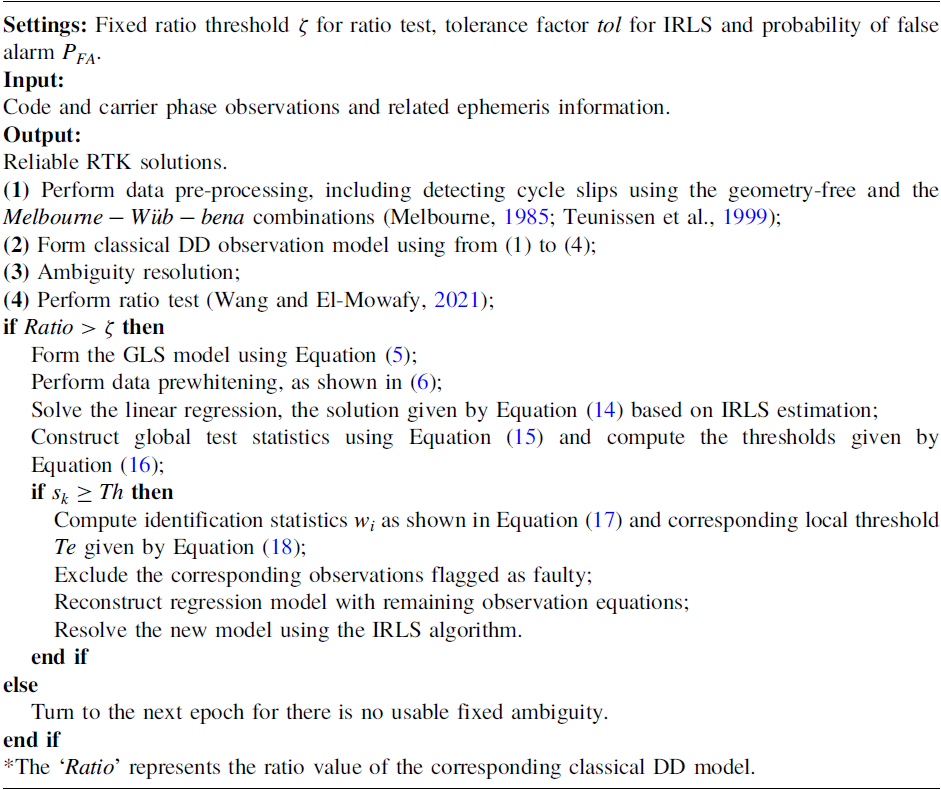
The key steps of improved fault detection and exclusion method based on the generalised least squares model for real-time kinematic positioning are listed in Algorithm 1.
Improved Fault Detection and Exclusion Method for RTK Positioning

4. Experiments and analysis
In this section, to validate the effectiveness of the proposed algorithm, a static test with artificial faults and a dynamic test with natural faults are carried out in ultra-short baseline RTK positioning scenarios. First, for the static test, basic dataset collection information and related faulty settings are introduced simply. Meanwhile, the performance of the presented method is analysed with simulated faults in detail. Then, for the dynamic test, considering the variation of fixed ambiguities due to the motion of the vehicle, two parallel experiments under different fixed ratio thresholds are implemented to illustrate the superiority of the proposed method with respect to classical LS in positioning performance. Moreover, test statistics of the enhanced FDE algorithm are also shown.
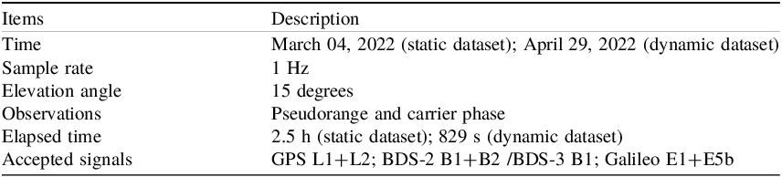
Table 1 describes the basic data collection information.
Description of dataset collection

4.1. Static test
4.1.1. Static dataset description
The static data was collected at 10:15 am on March 04, 2022, and lasted for 2.5 h. During the experimental test, two RTK static stations equipped with Trimble BD990 GNSS receivers were located on the roof of the building at Nanjing Intelligent Robot Industrial Park near the Jiulong Lake campus of Southeast University. The reference solutions were obtained from NovAtel Intertial Explorer 8.7 software in a smoothed RTK model.
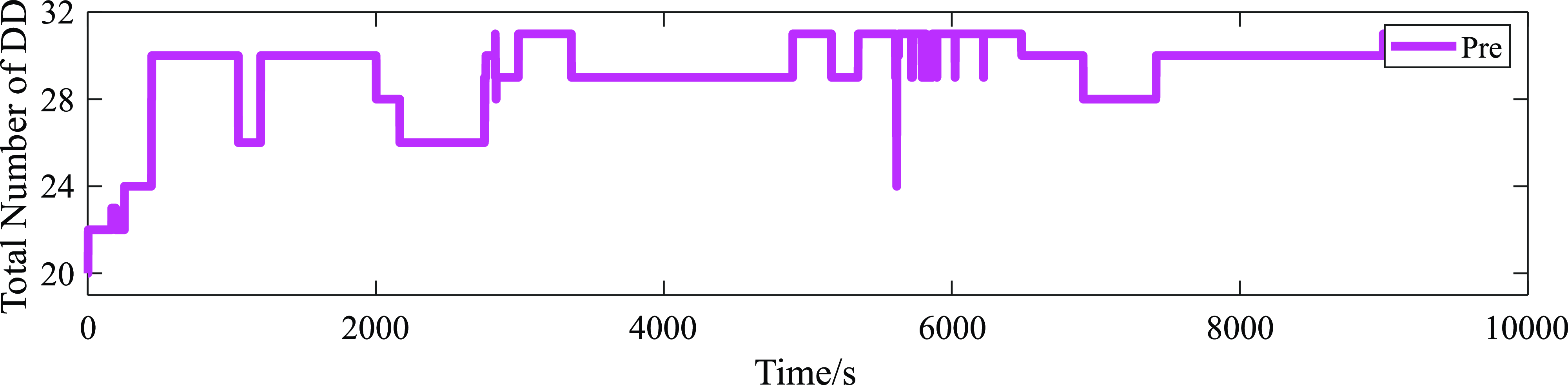
To provide a clear description of the experiment environment, the skyplot of the static dataset is shown in Figure 1. Meanwhile, the total number of DD equations and the evolution of GDOP and ratio values during the experimental test are given in Figures 2 and 3, respectively.
Skyplot of the static dataset.

Total number of usable DD equations of the static dataset.

GDOP (top) and ratio (bottom) of static dataset.

4.1.2. Performance evaluation
Before analysing algorithm performance, fault settings are described briefly.
-
1. Faults settings
To illustrate the performance of the presented algorithm, we add multiple faults to fixed ambiguities which are selected from the observations
 ${{\rm l}_k}$
given by Equation (5) and the time interval between adjacent faults is 2,000 s. It is noted that although the form of outliers is uncertain, caused by some adverse factors including the NLOS and multipath phenomenon, they are reflected on the DD equations with the form of wrong fixed ambiguities. These faulty fixed ambiguities with the nature of integer occur to different frequencies for the possibility of multiple faults on the same frequency is negligible to some extent. The amplitudes of corrupted observations are one circle in this static experiment because the number one is the smallest positive integer. If the smallest bias can be detected, blunders with large amplitudes are also able to be successfully excluded for a positioning system with given tolerance ability. Table 2 describes the fault profile in detail.
-
2. Performance evaluation
Simulation faults settings

In the given faulty scenario, the probability of false alarm is set to 0.0005. The global detection statistics are depicted in Figure 4, where the red line represents the evaluation of detection thresholds. Once the statistics exceed the corresponding detection thresholds, the positioning system is judged to have faults. As shown in the figure, the faults can be detected obviously four times at time points 2,000, 4,000, 6,000 and 8,000 s. It is illustrated that the added faults have been detected successfully by the proposed method. In addition, the test statistics are 2.15, 1.93, 2.38 and 2.58, and the corresponding critical thresholds are 1.464, 1.473, 1.455 and 1.464 at four detected faulty time points, respectively. The test statistic at time point 4,000 s is the smallest among the four test statistics for the number of simulated faults at this point equal to two with the same faulty amplitude.
Evaluation of global detection statistics (static dataset).

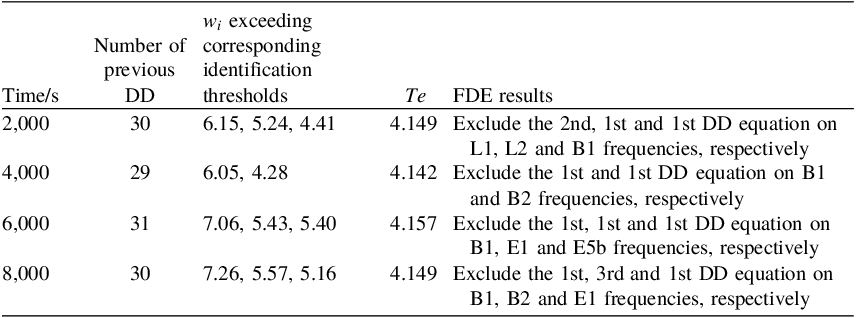
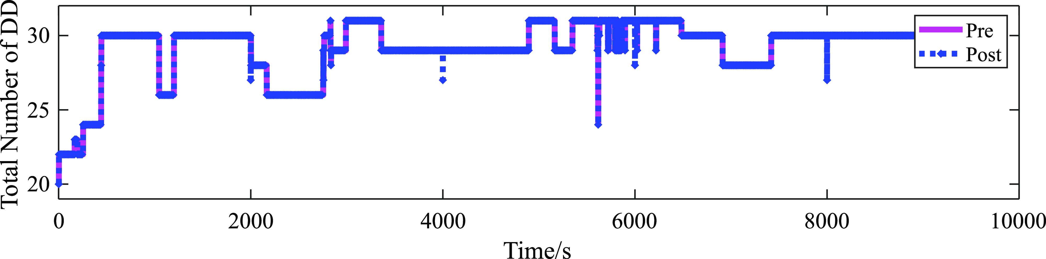
If the above global detection is not passed, the positioning system can locate the corresponding contaminated observations from the standardised observation model. These w-test statistics and identification thresholds and FDE results are listed at faulty time points in Table 3. The identification thresholds can be computed using Equation (18). There are 3, 2, 3, and 3 wrong fixed ambiguities at the faulty time points, and the corresponding DD equations for the occurrence of faulty observations are excluded correctly. In addition, Figure 5 depicts the total number of usable DD equations before and after using the improved FDE method. It is evident that the number of DD equations used (‘Pre’) is different from the number of DD equations (‘Post’) because the proposed method rejects blunders.
FDE information of static dataset with simulated faults

Total number of usable DD equations before and after using the improved method (static dataset).

Using the remaining normal standardised DD equations, the proposed method is able to be used to estimate the receiver position. The positioning errors in the east, north and upward (ENU) directions of our algorithm, as well as of the classical LS method, are shown in Figure 6. It is obvious that those errors of the above two methods during the normal times are basically consistent. In addition, the robust weight matrix of the IRLS algorithm could also eliminate the influences of several tiny blunders. Meanwhile, the traditional LS has no robustness to outliers and is easily disturbed by them at faulty times. Therefore, the appearance of the contaminated fixed ambiguities causes significant jitter in positioning errors from LS solutions, which seriously deviates from the fluctuation range of errors under normal times, especially the errors in upward direction. In contrast, the method presented in this paper can obviously reduce the adverse effects and keep the positioning errors in a relatively stable range in the same situations. Aimed at the east error at 6,000 s and north error at 8,000 s of the presented method, the influences of the erroneous fixed ambiguities on positioning have not been completely controlled. This is likely related to the selected faulty fixed integer ambiguities. The importance and contribution of each DD equation are different for positioning in ENU coordinates. The exclusion of important DD observations damaged the accuracy of positioning. The experimental results and analysis of the static dataset with artificial faults show that the proposed method not only improves positioning accuracy, but also ensures positioning robustness.
Positioning errors of classical LS and proposed method in east, north and upward directions (static dataset with simulated faults).

To illustrate the statistical difference between the above two kinds of errors clearly, Figure 7 gives the corresponding cumulative distribution function curves of three-dimensional (3D) positioning errors. It proves the superiority of the proposed algorithm. Specifically, for the same 3D positioning error, such as 0.025 m, the cumulative probability of the LS method is 56.78
 ${\rm{\% }}$
, while the corresponding probability of the proposed method is 59.99
 ${\rm{\% }}$
. It means that in the period of static experiment with 9,000 s, the errors of approximately 5,399 s can be guaranteed to be within 0.025 m using the method presented, while there are only errors of approximately 5,110 s under traditional LS estimation.
Cumulative distribution functions of classical LS and proposed method (static dataset with simulated faults).

Through adding simulated faults to the static dataset, it is shown that the proposed method can provide high-precision and high-reliability RTK solutions in the case of wrong fixed integer ambiguities by analysing test statistics of the enhanced FDE algorithm and comparing its positioning errors and CDF concerning classical LS.
4.2 Dynamic test
4.2.1 Dynamic dataset description
The dynamic vehicle data were collected on April 29, 2022, and lasted for approximately 14 min. During the experimental test, the RTK base station equipped with a Trimble BD990 GNSS receiver was located on the roof of the building at Nanjing Intelligent Robot Industrial Park. The rover station was set on the moving vehicle equipped with Unicorecomm um482. The vehicle test was implemented with a rectangle plot on the Jiulong Lake campus of Southeast University surrounded by a handful of buildings and trees on both sides of the road. The base station, rover station and trajectory of the dynamic test are shown in Figure 8. The reference solutions were obtained from NovAtel Intertial Explorer 8.7 software in smoothed RTK/INS tightly coupled mode.
Test trajectory of the dynamic dataset.

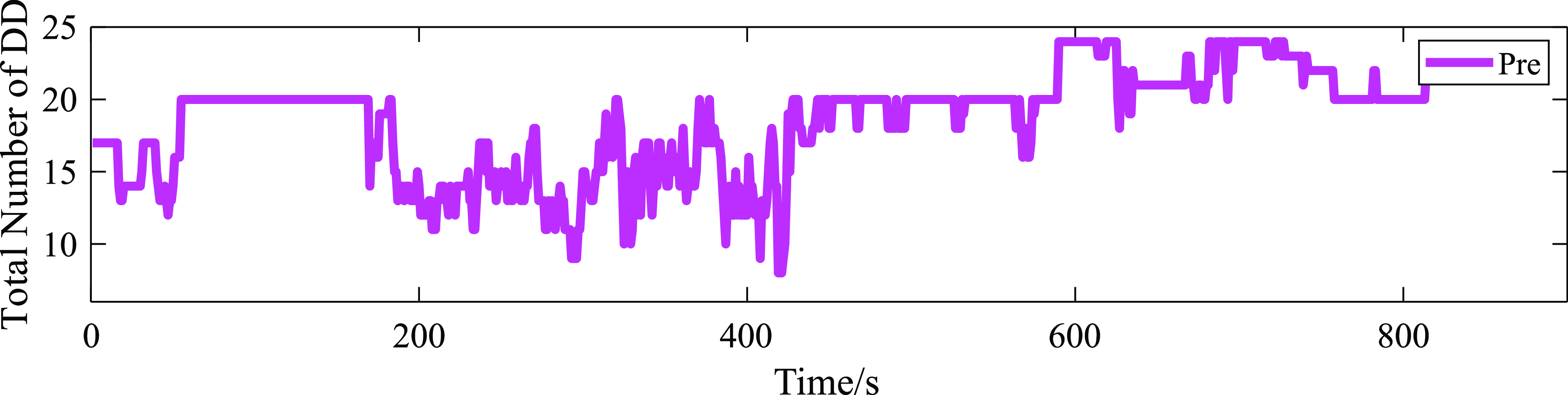
To provide an intuitive description of the experiment environment, the skyplot of the static dataset is shown in Figure 9. Meanwhile, the total number of DD equations and the evolution of GDOP and ratio values during the experimental test are depicted in Figures 10 and 11, respectively. It is obvious that, compared with other time points, the number of usable DD equations is less and changes dramatically, while the GDOP values increase significantly and the ratio values are relatively small during the period from 170 to 450 s. The main reason is that there exist obstacles around the vehicle during this period and blocked GNSS signals create a relatively challenging environment for RTK positioning.
Skyplot of dynamic dataset.

Total number of usable DD equations of the dynamic dataset.

GDOP (top) and ratio (bottom) of dynamic dataset.

4.2.2. Performance evaluation
Different from the steady collection environment of the static dataset, the ambiguity resolution in a dynamic test depends strongly on the operation environment of the vehicle. In addition, according to the basic principle of the ratio test, the fixed ratio threshold
 $\zeta $
given by Algorithm 1 is essential for the ambiguity fix rate. Table 4 provides corresponding fixed ambiguity information in three fixed ratio thresholds. In general, the high ambiguity fix rate is pursued with a low fixed ratio threshold. However, the thresholds with small amplitudes are easy to lead to wrong fixed ambiguities, resulting in unreliable RTK positioning solutions. In contrast, if the threshold value is too large, the fixed ambiguities cannot be used adequately. In practical applications, the selection of the ratio threshold is decided by the operation environment of the vehicle. Specifically, it can be appropriately reduced for a higher fixed rate and accuracy in more open environments. While the operation environment is relatively challenging, the threshold needs to be increased to improve the availability of fixed ambiguities as much as possible.
Fixed ambiguity information in different thresholds

To perform the method presented normally,
 $\zeta $
cannot be set too small due to the limited anti-faulty ability of fault detection and exclusion method based on the consistent check. Therefore, this part focuses on evaluating the special performance of the proposed method under the fixed ratio threshold of 2.0 and 1.2.
Considering the complication of the test environment and the growing risk of fixed ambiguities error, the probability of false alarm is set to 0.005 reasonably.
-
1.
 $\zeta $
=2.0

The global detection statistics under the fixed ratio threshold 2.0 of the vehicle test are depicted in Figure 12, where the blue curve is the evaluation of chi-square detection statistics and the red line represents corresponding detection thresholds. It is shown in the figure that natural faults on fixed ambiguities can be detected obviously at 466 s during the experimental test. The corresponding test statistic is equal to 1.52 and its critical value is 1.450. It is worth noting that the ratio value equals 9.504 at the faulty time detected, exceeding the ratio threshold significantly. Therefore, at 466 s, there exists a large possibility that these fixed integer ambiguities are accepted for high-precision RTK positioning. It is not reasonable, as shown in Figure 15. Such fault reflected in observations has been detected successfully by the proposed method. In addition, the test statistics in the dynamic test fluctuate dramatically compared with the corresponding detection in the static environment with artificial faults, especially for challenging periods, which are mainly caused by frequent satellite switching due to blocked obstacles.
Evaluation of global detection statistics (dynamic dataset,
 $\zeta $
=2.0).

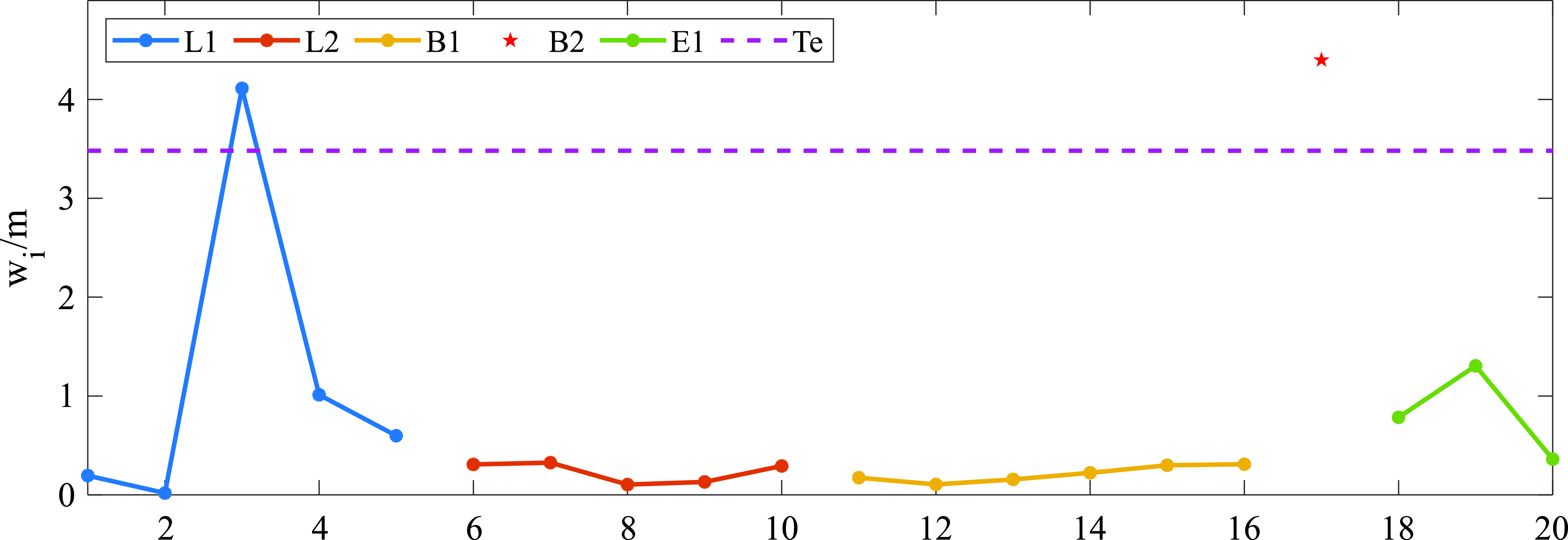
These w-test statistics and identification thresholds are depicted at faulty time point 466 s in Figure 13. In addition, Figure 14 shows the total number of usable DD equations before and after using the improved method in frequencies L1 and B1. The corresponding threshold equals 3.481 and there is no usable standardised DD equation in the frequency E5b. It can be known that at time point 466 s, the first and third observations on frequencies L1 and B1 occur with wrong fixed integer ambiguities. The corresponding DD equations for the occurrence of faulty ambiguities are rejected correctly, as shown in Figure 14.
Local identification statistics at time point 466 s (dynamic dataset,
 $\zeta $
=2.0).

Total number of usable DD equations before and after using the improved method at frequencies L1 and B1 (dynamic dataset,
 $\zeta $
=2.0).

Positioning errors of classical LS and proposed method in east, north and upward directions (dynamic dataset,
 $\zeta $
=2.0).

The positioning errors in the east, north and upward directions of our algorithm as well as of the classical LS method are shown in Figure 15, respectively. In addition, Figure 16 gives the corresponding CDF curves of 3D positioning errors to illustrate the statistical difference of two kinds of errors clearly. Similarly, errors of the above two methods during the normal times are basically consistent. Meanwhile, the robust weight matrix of the IRLS algorithm could also eliminate the influences of several tiny blunders that pass the FDE test, such as at time points 449 s and 485 s. In terms of upward error at 466 s, the error amplitude used by the traditional LS is raised to 0.08 m due to the contaminated fixed ambiguities, while such error is decreased to 0.014 m through the method presented. It further proves the superiority of the proposed algorithm as depicted in Figure 16.
Cumulative distribution functions of classical LS and proposed method (dynamic dataset,
 $\zeta $
=2.0).

2.
 $\zeta $
=1.2
Similarly, to further illustrate the performance of the presented algorithm, we provide the evolution of FDE test statistics and positioning errors under the fixed ratio threshold of 1.2 during the dynamic test in detail. Figure 17 shows global detection statistics and corresponding detection thresholds. On the one hand, it is shown that the number of statistics in the period of existing obstacles blocked is increased because of the growing ambiguity fix rate due to the decreased fixed ratio threshold. However, the low ratio threshold results in the risk of occurrence of wrong fixed ambiguities. On the other hand, apart from the time point 466 s, it is obvious that the chi-square statistic at 443 s is equal to 5.25, which exceeds the detection threshold with an amplitude of 1.450. Meanwhile, the corresponding ratio value at this point is 1.37. It is possible to cause a large deviation in positioning results if the fixed ambiguities at such a time are blindly used to estimate states. Fortunately, the proposed method can detect the existence of faults in time to prevent the positioning system from experiencing undesirable errors.
Evaluation of global detection statistics (dynamic dataset,
 $\zeta $
=1.2).

Specifically, there exist 20 usable DD equations at 443 s, so the corresponding identification threshold is equal to 3.481. In the frequency L1 with five usable DD equations, the w-test statistic with an amplitude of 20.84 located on the third observation is only identified as faulty. It can be justified that the corresponding fixed integer ambiguity is significantly wrong, which is intolerable for the centimetre-level positioning accuracy of RTK.
In terms of positioning errors, the relevant information is depicted in Figure 18. At the faulty epoch, the traditional LS directly uses wrong fixed ambiguities to locate the vehicle, and the positioning errors in east, north and upward directions are 0.05, 0.07 and 0.20 m, respectively, which deviate from the fluctuation range of errors in normal epochs. By adopting the relevant rejection operation, the corresponding errors are decreased to 0.001, −0.005 and 0.01 m, eliminating the adverse effect of blunders on accuracy and reliability performance. In addition, Table 5 and Figure 19 give the positioning errors comparison and the corresponding CDF curves of 3D positioning errors of the mentioned methods, to illustrate the superiority of the proposed algorithm from the standpoint of statistics.
Positioning errors of classical LS and proposed method in the east, north and upward directions (dynamic dataset,
 $\zeta $
=1.2).

Positioning errors comparison

Cumulative distribution functions of classical LS and proposed method (dynamic dataset,
 $\zeta $
=1.2).

By analysing test statistics of the enhanced FDE algorithm, and comparing its positioning errors and CDF concerning classical LS under two different fixed ratio thresholds, it is concluded that the proposed method can provide high-precision and high-reliability RTK solutions in the case of wrong fixed integer ambiguities due to observation faults.
5. Conclusions
To address the issue of unreliable ambiguity resolution due to observation faults, and ensure the accuracy and robustness of RTK positioning, an improved fault detection and exclusion method based on the generalised least squares model has been proposed in this paper. Through static tests with artificial faults and dynamic tests with natural faults in ultra-short baseline RTK positioning scenarios, the validity of the proposed method was demonstrated. The results show the following.
-
1. In static positioning scenarios with simulated faults, the proposed method can detect and exclude these DD equations with corrupted fixed ambiguities correctly. In terms of positioning errors, the appearance of the contaminated fixed ambiguities results in significant deviation about LS solutions, especially in the upward direction, while the method presented eliminates the adverse effects of blunders to a great extent.
-
2. In dynamic positioning scenarios with a fixed ratio threshold of 2.0, it is indicated that the first and third observations on frequencies L1 and B1 involve wrong fixed integer ambiguities at 466 s by means of the presented method.
-
3. In dynamic positioning scenarios with a fixed ratio threshold of 1.2, apart from the faults at 466 s, there still exists a single failure on the third observation in the frequency L1 at 443 s, which is identified by the proposed FDE method.
-
4. Compared with the positioning performance of traditional LS estimation of the dynamic test, the unique superiority of the presented algorithm is reflected in removing several tiny blunders as well as excluding observation faults that would be introduced in fixed ambiguities.
The above experiment results adequately indicate that the proposed method can provide high-precision and high-reliability RTK positioning solutions in the case of existing corrupted observation faults. However, the enhanced method is built on the GLS model, which is formed by the known fixed ambiguities. Therefore, we will extend the presented methods to more general situations for adapting different scenarios in the next work. In addition, for the continuity of positioning in complex environments, combining the RTK solutions provided by the proposed method with other navigation sensors is another work.
Acknowledgement
The authors would like to thank Professor Dequan Li of Anhui University of Science and Technology (AUST), for helpful discussions on the early stages of this work.
Funding statement
This work was supported by the Science and Technology Project of State Grid Corporation of China under Grant No. 5700-202140340A-0-0-00.