Quantitative predictions of cavitation presence and erosion-prone locations in a high-pressure cavitation test rig

Phoevos Koukouvinis; Nicholas Mitroglou; Manolis Gavaises; Massimo Lorenzi; Maurizio Santini

doi:10.1017/jfm.2017.156

Quantitative predictions of cavitation presence and erosion-prone locations in a high-pressure cavitation test rig

Published online by Cambridge University Press: 18 April 2017

and

Phoevos Koukouvinis*: Affiliation:
School of Mathematics Computer Science and Engineering, City University London, London EC1V 0HB, UK
Nicholas Mitroglou: Affiliation:
School of Mathematics Computer Science and Engineering, City University London, London EC1V 0HB, UK
Manolis Gavaises: Affiliation:
School of Mathematics Computer Science and Engineering, City University London, London EC1V 0HB, UK
Massimo Lorenzi: Affiliation:
School of Mathematics Computer Science and Engineering, City University London, London EC1V 0HB, UK
Maurizio Santini: Affiliation:
Department of Engineering and Applied Sciences, University of Bergamo, Bergamo, 24129, Italy
*: †Email address for correspondence: foivos.koukouvinis.1@city.ac.uk

Article contents

Abstract
Introduction
Experiment and simulation set-up
Numerical discretization, mesh convergence and uncertainty
Experimental and numerical results
Discussion
Conclusion
References

Rights & Permissions

Abstract

Experiments and numerical simulations of cavitating flow inside a single-orifice nozzle are presented. The orifice is part of a closed flow circuit, with diesel fuel as the working fluid, designed to replicate the main flow pattern observed in high-pressure diesel injector nozzles. The focus of the present investigation is on cavitation structures appearing inside the orifice, their interaction with turbulence and the induced material erosion. Experimental investigations include high-speed shadowgraphy visualization, X-ray micro-computed tomography (micro-CT) of time-averaged volumetric cavitation distribution inside the orifice as well as pressure and flow rate measurements. The highly transient flow features that are taking place, such as cavity shedding, collapse and vortex cavitation (also known as ‘string cavitation’), have become evident from high-speed images. Additionally, micro-CT enabled the reconstruction of the orifice surface, which provided locations of cavitation erosion sites developed after sufficient operation time. The measurements are used to validate the presented numerical model, which is based on the numerical solution of the Navier–Stokes equation, taking into account compressibility of both the liquid and liquid–vapour mixture. Phase change is accounted for with a newly developed mass transfer rate model, capable of accurately predicting the collapse of vaporous structures. Turbulence is modelled using detached eddy simulation and unsteady features such as cavitating vortices and cavity shedding are observed and discussed. The numerical results show agreement within validation uncertainty with the obtained measurements.

JFM classification

Drops and Bubbles: Cavitation Multiphase and Particle-laden Flows: Multiphase flow Vortex Flows: Vortex interactions

Information

Type: Papers
Information: Journal of Fluid Mechanics , Volume 819 , 25 May 2017, pp. 21 - 57
DOI: https://doi.org/10.1017/jfm.2017.156 [Opens in a new window]
Copyright: © 2017 Cambridge University Press

1 Introduction

Cavitation is the phenomenon of vaporous pocket formation inside liquids due to a drop in the local static pressure (Brennen Reference Brennen1995); it commonly appears in hydraulic pumps, turbines, propellers, rudders (Li Reference Li2000), in high-pressure fuel injection systems (Egler et al. Reference Egler, Giersch, Boecking, Hammer, Hlousek, Mattes, Projahn, Urner, Janetzky, Mollenhauer and Tschöke2010) and even heart valves (Kini et al. Reference Kini, Bachmann, Fontaine, Deutsch and Tarbell2000). Cavitation causes flow blockage and choking, while the collapse of cavitation structures may lead to cavitation erosion damage with detrimental consequences for the reliability and maintenance of relevant devices. Apart from the aforementioned effects, in the field of fuel injection systems, cavitation plays a detrimental role in jet formation, stability and atomization (Sou, Hosokawa & Tomiyama Reference Sou, Hosokawa and Tomiyama2007), affecting the combustion process and finally the performance and emissions of modern engines. For all of the previous reasons, significant effort has been put into the investigation of cavitating flows and prediction/quantification of related effects both with experimental and numerical/simulation techniques, in order to prevent negative aspects or to harness any positive potential (if applicable).

Cavitating flows have been extensively examined utilising high-speed shadowgraphy. An excellent summary of optical visualization techniques, involving schlieren, shadowgraphy and interferometry in the field of cavitation is discussed in the work of Mauger et al. (Reference Mauger, Méès, Michard, Azouzi and Valette2012) in a simplified, high pressure two-dimensional (2-D) channel. In the field of diesel injection systems, Mitroglou et al. (Reference Mitroglou, McLorn, Gavaises, Soteriou and Winterbourne2014) studied the flow in a real size diesel injector, whose metallic tip was removed and replaced with a transparent one, to conduct visualization studies. The study involved the realistic operation of the injector, under a pressure pulse of up to 600 bar, while observing cavitation formation in the sac and nozzles of the injector. The authors focused on unsteady cavitating features and especially the formation of cavitating vortices (which are also termed as ‘string cavitation’ in the fuel injection industry, due to their rope-like appearance), known to increase spray cone angles (Zigan et al. Reference Zigan, Schmitz, Wensing and Leipertz2012). Similarly, Hult et al. (Reference Hult, Simmank, Matlok, Mayer, Falgout and Linne2016) studied the cavitating flow in a marine diesel injector using high-speed shadowgraphy, among other techniques, for understanding the near nozzle jet behaviour and how this is affected by rolling vortex streets, formed at the edge of the orifice entrance. In general, such optical techniques are not limited to diesel injectors or fuel injection systems; for example, Pennings et al. (Reference Pennings, Bosschers, Weserweel and van Terwisga2015) used shadowgraphy for studying the formation, development and oscillation of a cavitating vortex emerging from the tip of a hydrofoil. Žnidarčič, Mettin & Dular (Reference Žnidarčič, Mettin and Dular2015) employed shadowgraphy to determine the extent of cavitation presence in the vicinity of an ultrasonic horn and compared the results with numerical simulations. At fundamental bubble dynamics, Lindau & Lauterborn (Reference Lindau and Lauterborn2003) studied the behaviour of laser bubble generation, growth and collapse in the vicinity of wall surfaces with high-speed shadowgraphy.

Despite the undoubted significance of optical methods as experimental techniques in understanding cavitation structures, their main drawback is that cavitation clouds, as observed from elastic scattering, do not correlate with the actual density of the liquid/vapour mixture. In addition, cavitation may obstruct the optical path, preventing further observation of flow features. For this reason, quantitative experimental techniques have been developed and employed to study and gain insight into the density distribution of cavitating flows. Such techniques rely on the attenuation of powerful photon or particle beams due to the presence of sample material along their path. Notable examples are neutron imaging (IAEA 2008) and X-ray imaging methods, which will be discussed later.

Two-dimensional X-ray radiography of cavitating flows in diesel injector orifices has been reported in simplified or even more complicated geometries. Duke et al. (Reference Duke, Kastengren, Swantek, Sovis, Fezzaa, Neroorkar, Moulai, Powell and Schmidt2014) studied a simple, axisymmetric nozzle of $500~\unicode[STIX]{x03BC}\text{m}$ diameter, using a powerful synchrotron X-ray source and compared the 2-D radiography projection of the vapour distribution with simulation results. Battistoni et al. (Reference Battistoni, Duke, Swantek, Tilocco, Powell and Som2015) employed a similar simplified geometry, but studied the effect of non-condensable gases (such as dissolved air in fuel) and the latter’s interaction with cavitation. Moon et al. (Reference Moon, Liu, Gao, Dufresne, Fezzaa and Wang2010) performed ultrafast X-ray phase contrast imaging for the identification of cavitation and spray boundaries emerging from a realistic multi-hole diesel injector. Further notable examples of works of a similar nature, but with different application fields, involve the study of cavitating flow around a NACA009 hydrofoil (Ganesh, Mäkiharju & Ceccio Reference Ganesh, Mäkiharju and Ceccio2016) using high-speed X-ray radiography, where compressibility effects during the collapse of attached cavitation clouds (condensation shocks) have been identified. Such effects are difficult, if not impossible, to identify with traditional optical measurements since the density field is not directly reproducible. In the same spirit, Sun, Ganesh & Ceccio (Reference Sun, Ganesh and Ceccio2015) studied the cavitating flow emerging from vortex shedding in the wake of a cylinder at conditions ranging from cavitation inception to supercavitation regimes. X-ray imaging can provide valuable information in more industrial cases as well; Duplaa et al. (Reference Duplaa, Coutier-Delgosha, Dazin and Bois2013) examined cavitation formation around the impeller of a pump during fast start-up operation and correlated the density variations to pressure time evolution.

While undeniably 2-D X-ray radiography can shed light on the instantaneous density distribution of the flow, it cannot provide information on the exact 3-D cavity shape. For this reason, Bauer, Chaves & Acroumanis (Reference Bauer, Chaves and Acroumanis2012) examined the flow inside an axisymmetric nozzle at cavitation numbers ranging from inception to supercavitation with X-ray computed tomography (CT). In their investigation, the working fluid was water and a medical scanner was utilized for the measurements. The CT scans enabled a 3-D volumetric reconstruction of the vapour cloud inside the orifice, which has been used for validation of computational fluid dynamics (CFD) codes that have been previously developed Giannadakis, Gavaises & Arcoumanis (Reference Giannadakis, Gavaises and Arcoumanis2008).

Simulation of cavitating flows is of high complexity due to the large density ratios involved and flow unsteadiness. Andriotis, Gavaises & Arcoumanis (Reference Andriotis, Gavaises and Arcoumanis2008) showed that turbulence can play a detrimental role in the flow development. Cavitating vortices, or ‘string cavitation’, were identified to affect the flow inside injector nozzle holes and the emerging jet. In more recent works, the effect of an accurate turbulence description is highlighted in the work of Edelbauer, Strucl & Morozov (Reference Edelbauer, Strucl, Morozov, Gourbesville, Cunge and Caignaert2016). The authors focused on fundamental investigation of microchannel flows at high pressures, showing the situational applicability of Reynolds-averaged Navier–Stokes (RANS)/unsteady Reynolds-averaged Navier–Stokes (URANS) models in describing cavitation effects at cavitation inception conditions. More recently Örley et al. (Reference Örley, Hickel, Schmidt and Adams2016) have achieved an impressive simulation of a complete 9-hole diesel injector, including injection in an air environment, aiming to study the influence of cavitation on the emerging jets. The work of Koukouvinis et al. (Reference Koukouvinis, Gavaises, Li and Wang2016) focused instead on the prediction of cavitation inside industrial diesel injector designs operating at similar conditions, while tracking the collapse of cavitation structures for correlation with the erosion development that was found from X-ray topography of used injectors.

Despite the numerous examples of numerical work, validation of relevant simulation models is not straightforward. Commonly it is done by comparing macroscopic quantities, such as flow rate or examining the unsteady patterns of cavitation structures in comparison to high-speed imaging. The present investigation aims to examine the cavitating flow in diesel injector-like geometries on a fundamental level. Similar to the work of Bauer et al. (Reference Bauer, Chaves and Acroumanis2012), the cavitating flow inside a cylindrical nozzle is investigated. However, in the present work, the orifice is placed asymmetrically with respect to upstream elements (e.g. the throttling needle), forcing the flow to be non-axisymmetric, forming a configuration that resembles more closely the flow path of a diesel injector. Despite the apparent simplicity of the experimental configuration and the stationary needle, notable flow effects occurring in real-world fuel injection systems, such as the formation of cavitating vortices and cavitation induced surface erosion, have been observed. Understanding these effects is crucial for the performance of a fuel injection system, since unsteady cavitating vortices affect jet atomization and spray patterns (Andriotis et al. Reference Andriotis, Gavaises and Arcoumanis2008; Giannadakis et al. Reference Giannadakis, Gavaises and Arcoumanis2008) and consequently engine performance, whereas material erosion can lead to performance deterioration, very high maintenance costs and reliability issues. It is highlighted that these effects are not limited to fuel systems, but have a general interest from a broad fluid dynamics perspective. The dynamics of cavitating vortices is discussed extensively in Franc & Michel (Reference Franc and Michel2005), who showed that circulation leads to a rebounding behaviour of a cavitating vortex, even in the absence of non-condensable gases, due to conservation of angular momentum. In real life, cavitating vortices occur in a wide range of engineering applications, such as at the tips of hydrofoils (Arndt, Arakeri & Higuchi Reference Arndt, Arakeri and Higuchi1991; Pennings et al. Reference Pennings, Bosschers, Weserweel and van Terwisga2015) or propeller blades (Duttweiler & Brennen Reference Duttweiler and Brennen2002) and contribute to the erosion of ship propellers and rudders (Carlton Reference Carlton2012) or the operation of hydro-turbines (Decaix et al. Reference Decaix, Balarac, Dreyer, Farhat and Münch2015). The aforementioned non-exhaustive list of references indicates the importance and need for an accurate and validated numerical model, capable of predicting cavitating vortex and cavitation erosion effects in a quantitative way.

The focus of the present paper is on the unsteady cavitating phenomena occurring inside the orifice, with emphasis on the formation of cavitating vortices, the interaction of the cavitation with turbulence and the mechanism that causes erosion in affected regions. The flow is studied experimentally and numerically. From the experimental side, high-speed shadowgraphy and time-averaged X-ray micro-CT scanning are employed. Numerical simulations complement the experimental results, providing additional insight, due to the complexity of the flow field which inevitably obstructs detailed observations in the whole flow passage. The objective of the present study is to obtain quantitative experimental data on both cavitation distribution and cavitation erosion sites, for a given orifice geometry (see also supplementary material available at https://doi.org/10.1017/jfm.2017.156) and operating conditions. These data may be further used for quantitative comparisons with numerical simulations, hence serving as a benchmark/validation case. Moreover, a cavitation model is discussed and validated against the aforementioned data, showing the main flow mechanisms and the outcome of the modelling approach. The novelty of the current work is the combined presentation of new experimental results, including 3-D density and cavitation erosion measurements, accompanied by numerical simulations of the relevant phenomena occurring in this flow orifice at low and high cavitation numbers. In particular, X-ray micro-CT cavitation volume fraction measurements, high-speed flow visualization and cavitation erosion areas are used for the detailed quantitative validation of the proposed cavitation model. The latter has been used in recent studies in predicting erosion locations in high pressure fuel injectors, see Koukouvinis et al. (Reference Koukouvinis, Gavaises, Li and Wang2016).

The paper is organized as follows: initially, the experimental test rig is described, along with details of the actual orifice geometry and operating conditions. Next, the numerical models used for the simulations, fluid properties and simulation set-up are discussed. Then, flow details from simulations are provided, such as visualization of cavitation, flow field and vortical structures. Next, the experimental and numerical results are compared, both in qualitative (e.g. vapour fraction isosurface shape) and quantitative terms (e.g. mass flow rate, vapour cavity extent, etc.). Finally, a short discussion of the results is made and main conclusions are summarized, highlighting the most important findings.

2 Experiment and simulation set-up

The geometry employed in the present study resembles the features of a diesel injector orifice and more specifically, it was designed to resemble the asymmetric flow of valve covered orifice (VCO) or mini-sac-type nozzles, inspired from the work of Reid et al. (Reference Reid, Hargrave, Garner and Wigley2010).

2.1 The experimental test rig

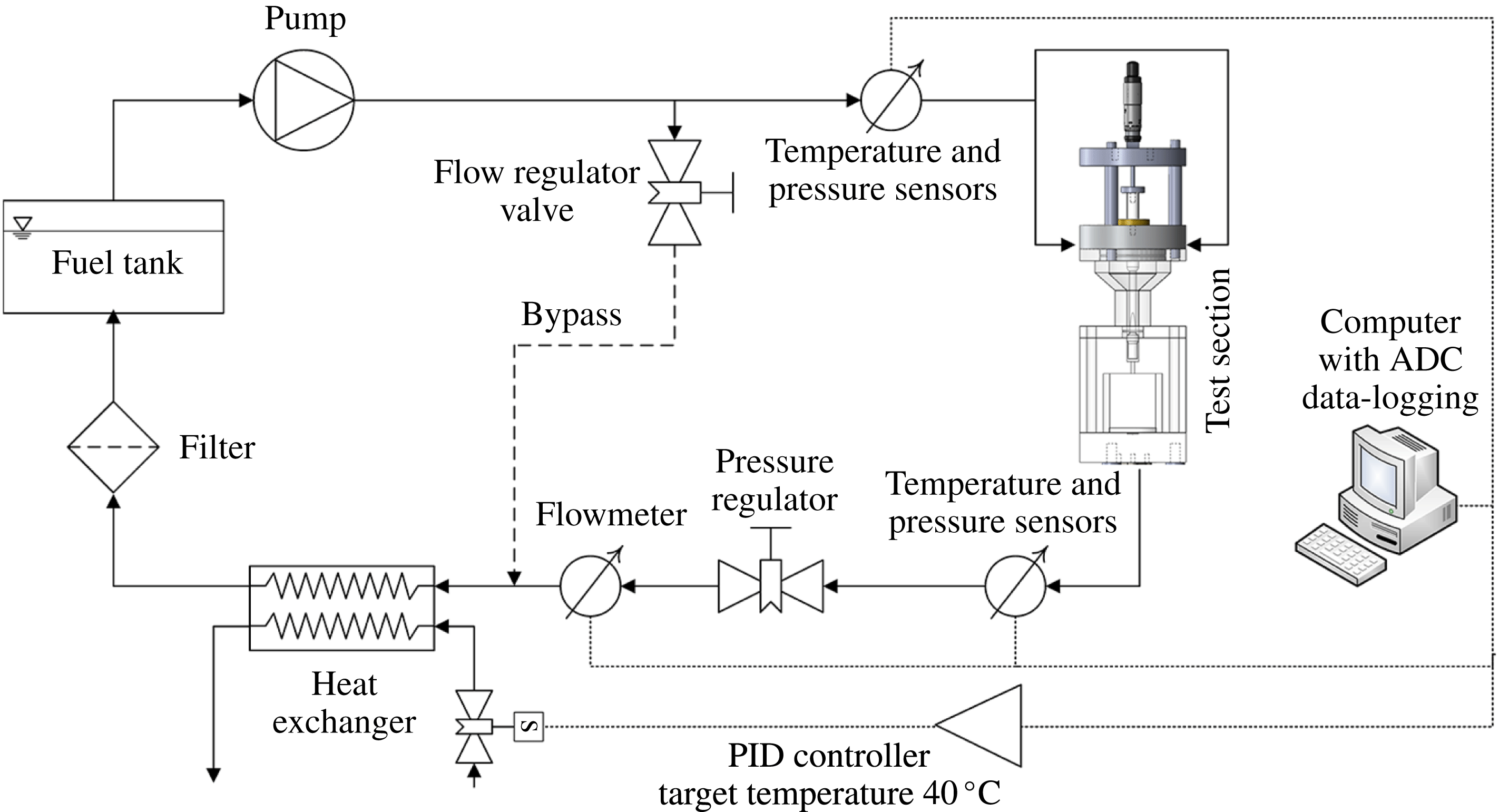
The experimental test rig consists of a closed loop hydraulic circuit (see also figure 1), comprised of a high-pressure hydraulic unit that circulates the flow, valves and pressure regulators to regulate flow rate and upstream/downstream pressure, the orifice test section and a shell and tube water-cooled heat exchanger to maintain a constant diesel fuel temperature. The hydraulic circuit also includes filters for controlling diesel quality, a fuel tank where fuel rests at low velocities, allowing any bubbles to escape, and the necessary piping. Pressure, temperature and flow rate are measured with appropriate transducers, connected to a computer via an analogue to digital converter (ADC) card for data logging.

Figure 1.

Single-line diagram of the hydraulic rig circuit.

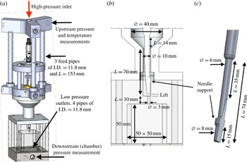
A view of the cavitation test section is shown in figure 2(a–c). Following the flow from the high pressure inlet towards the low-pressure outlet, the test section consists of a high pressure inlet socket, which is split to three feed lines, figure 2(a). This arrangement was used to accommodate adjustable needle lift for controlling the flow rate with higher precision. The feed lines converge to a funnel shaped passage that further downstream becomes annular; inside this passage the needle is located. Note that, even though the needle is cylindrical upstream of the funnel, it becomes asymmetrical near the orifice entrance due to a bevel cut at its tip and the support structure that is in contact with the passage walls, blocking part of the flow. The orifice is placed off-axis, to further promote flow asymmetry, on an interchangeable part that includes also the collector volume. Downstream the collector are four low-pressure outlet pipes, that direct the flow to the return of the hydraulic unit.

Figure 2.

(a) Drawing of the experimental test section, (b) focused view in the area of interest with main dimensions, (c) drawing of the needle and relevant dimensions.

The interchangeable part, that includes the orifice itself, allows for different types of flow investigations to be conducted. For visualization studies, the orifice was made of a transparent acrylic resin piece with rectangular collector, see figure 2(b), whereas for the X-ray investigation the orifice was drilled on a polyether ether ketone (PEEK) piece with cylindrical collector (not shown here). The idealized orifice examined here is a cylinder of 9.5 mm length and 3 mm diameter.

The two cases that have been examined experimentally and numerically are outlined in table 1; two common cavitation number definitions are provided according to

(2.1)

$$\begin{eqnarray}Cn=\frac{1}{\unicode[STIX]{x1D70E}}=\frac{p_{up}-p_{down}}{p_{down}-p_{v}},\end{eqnarray}$$

where $p_{up}$ is the upstream pressure, $p_{down}$ the downstream pressure and $p_{v}$ the vapour (or saturation) pressure. Reynolds number is defined as

(2.2)

$$\begin{eqnarray}Re=\frac{u_{avg}D\unicode[STIX]{x1D70C}_{l}}{\unicode[STIX]{x1D707}_{l}},\end{eqnarray}$$

where $u_{avg}$ is the average velocity in the orifice cross-section, assuming it is fully occupied by liquid, $D$ is the orifice diameter, $\unicode[STIX]{x1D70C}_{l}$ is the liquid density and $\unicode[STIX]{x1D707}_{l}$ liquid viscosity.

Table 1.

Operating conditions for two of the cases examined with experiment and simulation. All cases are at 1 mm needle lift. Average velocity is estimated inside the orifice cross-section assuming the whole cross-section is occupied by liquid.

Both cases correspond to the same needle lift of 1 mm from the fully closed position and to two different cavitation numbers, at $Cn=2.18$ and $Cn=1.5$ , which will be referred to as high and low cavitation intensity, respectively. For the whole duration of the experiments, fuel temperature was controlled at $40\pm 0.5\,^{\circ }\text{C}$ . Errors reported in table 1 are based on systematic and random measurement errors of the pressure and flow transducers and error propagation analysis for the derived values (e.g. cavitation number, Reynolds number), see Bevington & Robinson (Reference Bevington and Robinson2003). The accuracy of the pressure transducers is 0.4 bar upstream, 0.17 bar downstream and their temporal resolution is 1 ms. The accuracy of the flow meter is $0.1~\text{l}~\text{min}^{-1}$ .

Shadowgraphy was employed as a visualization technique for capturing still images of the transient cavitation structures emerging inside the orifice. The experimental set-up of the image acquisition methodology is comprised of a halogen floodlight providing white band light, which was subsequently focused by a Fresnel lens on the area of interest. The placement of a charge-coupled device (CCD) camera at the opposite side of the device allowed for side view images of the arising vapour cloud to be taken. A high-speed Photron SA-X camera was employed, adjusted to capture 80 000 frames per second (f.p.s.) at a resolution of $896\times 264$ pixels. The shutter speed was set to $0.37~\unicode[STIX]{x03BC}\text{s}$ to increase image clarity and ‘freeze’ the high-velocity flow phenomena inside the orifice. Since the overall length of the visualized orifice region is equal to 10 mm and 646 out of the total 896 pixels are employed for its discretization, the visualization resolution is equal to $15.47~\unicode[STIX]{x03BC}\text{m}~\text{pixel}^{-1}$ . The resolution of the visualization technique is of the order of the manufacturing uncertainty associated with the orifice dimensions, while the size of cloud cavitation and coherent cavitating vortices are much larger and comparable to the orifice diameter ( ${\sim}3.0~\text{mm}$ ). Hence, the spatial resolution is sufficient for properly illustrating the topology of the two-phase flow in the area of interest.

The prototype micro-CT facility (located at the University of Bergamo) employed for cavitation volume fraction measurements and orifice surface deformation measurements consists of a 160 kV (at $400~\unicode[STIX]{x03BC}\text{A}$ ) open-type cone-beam X-ray source, an air-bearing direct drive rotary stage and a $1944\times 1536$ pixel flat panel complementary metal–oxide–semiconductor (CMOS) detector with a custom matched scintillator plate. The spatial resolution was adapted to provide an isotropic voxel size of $15~\unicode[STIX]{x03BC}\text{m}$ (in the reconstructed volume). For each of the 600 steps required for a full rotation of the test item, five projections were acquired and averaged to improve the signal to noise ratio. The full scan time for each test case was approximately equal to one hour, since a projection acquisition time of 1000 ms was used. During the image acquisition, no beam filtration was applied to the incoming X-rays produced by the source, which was set to 60 kV and $40.2~\unicode[STIX]{x03BC}\text{A}$ . Further details regarding the experimental procedure utilized are documented in more detail in Mitroglou et al. (Reference Mitroglou, Lorenzi, Santini, Gavaises and Assanis2015). The reconstruction algorithm employed is based on the work of Feldkamp, Davis & Kress (Reference Feldkamp, Davis and Kress1984). Experimental errors of the density reconstruction were estimated using the standard deviation of the density for air–liquid calibration and were approximately 4 %.

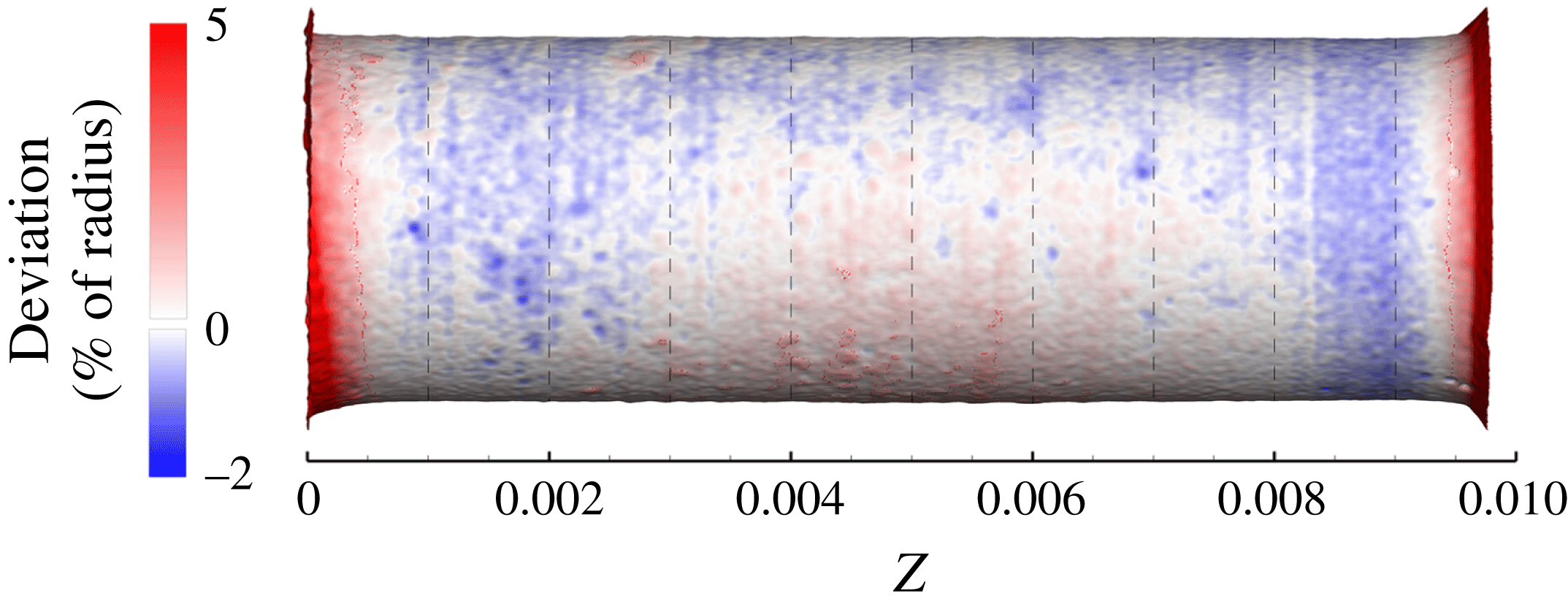
In practice, the orifice dimensions were not perfectly cylindrical due to manufacturing defects but also due to self-induced hydro-grinding of the sharp features, occurring during the early testing of the operation of the device. This resulted in an up to 10 % difference in the measured (as well as the calculated) flow rate through the orifice, relative to the ideal cylindrical, sharp edge shape. Nevertheless, the resulting geometry was stabilized and remained unchanged after a short operating time; its shape is shown in figure 3. ANSA (Stampouli & Pappas Reference Stampouli and Pappas2014) and MeshLab (Cignoni et al. Reference Cignoni, Callieri, Corsini, Dellepiane, Ganovelli and Ranzuglia2014) software were used for cleaning and manipulating the CT scan geometry and obtaining computer-aided design (CAD) representations (shown in figures later on) and for meshing. The actual orifice geometry has an average radius of $R_{av}=1503~\unicode[STIX]{x03BC}\text{m}$ with a standard deviation $\unicode[STIX]{x1D70E}_{R}=14.7~\unicode[STIX]{x03BC}\text{m}$ from an ideal cylinder. Considering the spatial resolution of the X-ray scan ( $\unicode[STIX]{x1D700}=15~\unicode[STIX]{x03BC}\text{m}$ ), the total error of the geometry representation is $\pm 46~\unicode[STIX]{x03BC}\text{m}$ (estimated as $\pm \sqrt{(3\unicode[STIX]{x1D70E}_{R})^{2}+\unicode[STIX]{x1D700}^{2}}$ for 99.7 % level of confidence (Bevington & Robinson Reference Bevington and Robinson2003)), or ${\sim}\pm 1.5\,\%$ of the nominal diameter. The CT-scanned orifice geometry has been used for the numerical simulations in order to take into account any geometry deviations that can affect the flow pattern, such as the smooth orifice entrance due to hydro-grinding. Prior investigation has shown that using an idealized cylindrical orifice with sharp turns at the entrance can lead to a severe underestimation of the flow rate.

Figure 3.

Close up view at the orifice, coloured according to the deviation from ideal cylinder; a smooth transition is visible at the orifice entrance, at the bottom left. Flow moves from left to right.

2.2 Simulation model and methodology

The numerical methodology used in the present work is based on the mixture level approach, i.e. the mixture continuity (2.3) and momentum equations (2.4) are solved:

(2.3)

$$\begin{eqnarray}\displaystyle & \displaystyle \frac{\unicode[STIX]{x2202}\unicode[STIX]{x1D70C}}{\unicode[STIX]{x2202}t}+\unicode[STIX]{x1D735}\boldsymbol{\cdot }(\unicode[STIX]{x1D70C}\boldsymbol{u})=0 & \displaystyle\end{eqnarray}$$

(2.4)

$$\begin{eqnarray}\displaystyle & \displaystyle \frac{\unicode[STIX]{x2202}\unicode[STIX]{x1D70C}\boldsymbol{u}}{\unicode[STIX]{x2202}t}+\unicode[STIX]{x1D735}\boldsymbol{\cdot }(\unicode[STIX]{x1D70C}\boldsymbol{u}\otimes \boldsymbol{u})=-\unicode[STIX]{x1D735}p+\unicode[STIX]{x1D735}\boldsymbol{\cdot }\unicode[STIX]{x1D749}, & \displaystyle\end{eqnarray}$$

where $\unicode[STIX]{x1D70C}$ is the mixture density, $\boldsymbol{u}$ is the velocity vector, $p$ is pressure and $\unicode[STIX]{x1D749}$ denotes the stress tensor, as described below:

(2.5)

$$\begin{eqnarray}\unicode[STIX]{x1D749}=\unicode[STIX]{x1D707}_{eff}[\unicode[STIX]{x1D735}\boldsymbol{u}+(\unicode[STIX]{x1D735}\boldsymbol{u})^{\text{T}}]+\unicode[STIX]{x1D706}(\unicode[STIX]{x1D735}\boldsymbol{\cdot }\boldsymbol{u})\unicode[STIX]{x1D644},\end{eqnarray}$$

with $\unicode[STIX]{x1D707}_{eff}$ the total effective viscosity of the mixture, including laminar, $\unicode[STIX]{x03BC}$ , and eddy viscosity, $\unicode[STIX]{x1D707}_{t}$ , contributions and $\unicode[STIX]{x1D644}$ is the identity matrix. The effect of bulk viscosity, $\unicode[STIX]{x1D706}$ , is omitted from equation (2.4), due to lack of data for diesel fuel; in any case, bulk viscosity only acts in passing waves so its effect on the general dynamics of the flow is negligible. In the present study, turbulence effects are taken into account with an improved delayed detached eddy simulation model (IDDES), which is a blend of RANS ( $k$ - $\unicode[STIX]{x1D714}$ shear stress transport (SST)) and a large eddy simulation (LES) Smagorinsky-like model (Mockett Reference Mockett2007; Shur et al. Reference Shur, Spalart, Strelets and Travin2008), depending on the mesh spacing and the local turbulent length scale. Such a treatment allows for low resolution in areas where there is little interest, such as upstream of the annular passage or downstream of the collector, reducing the computational cost since it reverts to the $k$ - $\unicode[STIX]{x1D714}$ SST model. On the other hand, in areas of adequate resolution, the model switches to a Smagorinsky-like subgrid model, enabling the accurate reproduction of turbulent structures, which have been shown in previous studies to be crucial in describing cavitation shedding and unsteadiness (Coutier-Delgosha, Reboud & Delannoy Reference Coutier-Delgosha, Reboud and Delannoy2003; Edelbauer et al. Reference Edelbauer, Strucl, Morozov, Gourbesville, Cunge and Caignaert2016).

Cavitation is tracked with a transport equation for the vapour fraction $a$ , which has the general form of

(2.6)

$$\begin{eqnarray}\frac{\unicode[STIX]{x2202}(a\unicode[STIX]{x1D70C}_{v})}{\unicode[STIX]{x2202}t}+\unicode[STIX]{x1D735}\boldsymbol{\cdot }(a\unicode[STIX]{x1D70C}_{v}\boldsymbol{u})=R_{e}-R_{c},\end{eqnarray}$$

where $\unicode[STIX]{x1D70C}_{v}$ is the vapour density and $R_{e}$ and $R_{c}$ are mass transfer terms associated with the evaporation and condensation of vapour. In this work, we propose a different formulation of the evaporation and condensation terms from existing cavitation models, as follows:

(2.7)

$$\begin{eqnarray}\displaystyle & \displaystyle R_{e}=F\left(1-a\right)\unicode[STIX]{x1D70C}_{v}\sqrt{\frac{2}{3}\frac{\max (p_{v}-p,0)}{\unicode[STIX]{x1D70C}_{l}}} & \displaystyle\end{eqnarray}$$

(2.8)

$$\begin{eqnarray}\displaystyle & \displaystyle R_{c}=Fa\unicode[STIX]{x1D70C}_{v}\sqrt{\frac{2}{3}\frac{\max (p-p_{v},0)}{\unicode[STIX]{x1D70C}_{l}}}, & \displaystyle\end{eqnarray}$$

where $\unicode[STIX]{x1D70C}_{l}$ is the liquid density and $F$ is the ratio of available interfacial surface area (in $\text{m}^{2}$ ) for mass transfer per unit volume (in $\text{m}^{3}$ ) of fluid; its units are $\text{m}^{-1}$ . The formulation of the mass transfer terms is based on the Zwart, Gerber & Belamri (Reference Zwart, Gerber and Belamri2004) model (see also Bakir et al. Reference Bakir, Rey, Gerber, Belamri and Hutchinson2004), however there are several fundamental differences. First of all, the aforementioned mass transfer model can be considered as a thermodynamic non-equilibrium model, since metastable conditions of liquid tension may develop if the mass transfer is low, as in e.g. the original Zwart et al. (Reference Zwart, Gerber and Belamri2004) formulation. On the other hand, if the mass transfer is sufficiently high, theoretically tending to infinity, as proposed in the present work, the two-phase model tends asymptotically to a barotropic cavitation model behaviour as in e.g. shock tube (Koukouvinis & Gavaises Reference Koukouvinis and Gavaises2015) or Rayleigh collapse tests (Koukouvinis, Naseri & Gavaises Reference Koukouvinis, Naseri and Gavaises2016). Adopting such an approach has several advantages.

(i) It can inherently predict the Rayleigh collapse of a vapour structure. As a comparison, cavitation models such as the baseline (Zwart et al. Reference Zwart, Gerber and Belamri2004) or Schnerr & Sauer (Reference Schnerr and Sauer2001) models may seriously overpredict the collapse time of a vaporous bubble due to the very small mass transfer rate (Koukouvinis et al. Reference Koukouvinis, Naseri and Gavaises2016).
(ii) The amount of unphysical tension in the liquid volume is significantly reduced and the minimum pressure is much closer to the vapour pressure (Koukouvinis et al. Reference Koukouvinis, Naseri and Gavaises2016). Again, the aforementioned cavitation models may predict liquid tension up to two orders of magnitude higher than the present model (Koukouvinis et al. Reference Koukouvinis, Gavaises, Li and Wang2016).
(iii) The approach of the model resembles a thermodynamic equilibrium assumption for cavitation, i.e. pressure in the cavitation zone is practically equal to the vapour pressure, which is supported by experimental data in the literature, see e.g. Washio (Reference Washio2014).
(iv) There is only a single tuning factor, $F$ , instead of four as in the original Zwart et al. (Reference Zwart, Gerber and Belamri2004) model. Moreover, its value is a priori known since, in order to be at thermodynamic equilibrium, it should be theoretically infinite. Obviously an infinite value is not possible for the numerical solver to handle, and very high values will cause serious numerical difficulties. However, since there is asymptotic convergence with the increase of $F$ towards thermodynamic equilibrium, extreme values are not needed; in practical cases, such as the one described here, values of $F$ of the order of $10^{8}$ $\text{m}^{-1}$ are adequate to maintain numerical stability and prevent liquid tension from becoming unphysical.

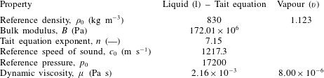
In the simulations presented here, the liquid phase is modelled as a compressible liquid, with the Tait equation of state:

(2.9)

$$\begin{eqnarray}\displaystyle & \displaystyle p=B\left[\left(\frac{\unicode[STIX]{x1D70C}}{\unicode[STIX]{x1D70C}_{0}}\right)^{n}-1\right]+p_{ref} & \displaystyle\end{eqnarray}$$

(2.10)

$$\begin{eqnarray}\displaystyle & \displaystyle B=\frac{\unicode[STIX]{x1D70C}_{0}c_{0}^{2}}{n}, & \displaystyle\end{eqnarray}$$

where $B$ is the bulk modulus, $\unicode[STIX]{x1D70C}_{0}$ is the reference density, $c_{0}$ is the reference speed of sound at reference density, $p_{ref}$ is a reference pressure (here equal to the vapour pressure $p_{v}$ ) and $n$ is an exponent adjusting the stiffness of the liquid. The values used are shown in table 2 and were chosen based on a diesel property library (Kolev Reference Kolev2007), at the temperature of the experiment ( $40\,^{\circ }\text{C}$ ). While the operating pressure levels, as shown in table 1, are not high enough to justify a compressible treatment of the liquid, the collapse of vaporous cavities induces locally very high pressures, of the order of 1000 bar, and compressibility becomes important. Moreover, numerical handling would be problematic the instant vapour disappears completely at the end of the collapse of a vaporous structure if the incompressible assumption was to be enforced, since liquid converges to a singular point with high velocity, obviously violating the incompressibility assumption of $\text{div}(\boldsymbol{u})=0$ . Vapour properties were assumed to be constant, based on saturation conditions at $40\,^{\circ }\text{C}$ .

Table 2.

Fluid properties used for the simulations presented hereafter. Properties are estimated at $40\,^{\circ }\text{C}$ , based on the work of Kolev (Reference Kolev2007).

Despite vapour density being assumed constant, the liquid/vapour mixture is highly compressible due to mass transfer terms. In the simulations to be presented, the speed of sound, $c$ , varies from the liquid speed of sound ( $c_{l}\sim 1200~\text{m}~\text{s}^{-1}$ ) to $0.01~\text{m}~\text{s}^{-1}$ in the cavitating mixture region, depending on the local mass transfer from liquid to vapour ( $\unicode[STIX]{x1D6FF}m$ , kg per m $^{3}$ of mixture) and pressure change, $\unicode[STIX]{x1D6FF}p$ , see Franc & Michel (Reference Franc and Michel2005):

(2.11)

$$\begin{eqnarray}\frac{1}{\unicode[STIX]{x1D70C}c^{2}}\cong \frac{1-a}{\unicode[STIX]{x1D70C}_{l}c_{l}^{2}}+\frac{a}{\unicode[STIX]{x1D70C}_{v}c_{v}^{2}}-\frac{\unicode[STIX]{x1D6FF}m}{\unicode[STIX]{x1D6FF}p}\left(\frac{1}{\unicode[STIX]{x1D70C}_{v}}-\frac{1}{\unicode[STIX]{x1D70C}_{l}}\right).\end{eqnarray}$$

Mixture compressibility affects the collapse of cavities; a high mass transfer rate (i.e. large absolute value of $\unicode[STIX]{x1D6FF}m/\unicode[STIX]{x1D6FF}p$ ) leads to a very low speed of sound within the mixture and supersonic cavity collapse (supersonic in terms of mixture speed of sound inside the cavity, not the liquid speed of sound). Thus during the collapse, pressure within the cavity remains approximately equal to the vapour pressure since no information can propagate in the liquid/vapour mixture, leading to the well-known Rayleigh collapse behaviour. A small mass transfer rate will render the mixture stiffer, preventing a violent cavity collapse.

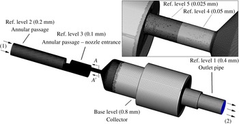
For the computational model, upstream elements of the annular passage have been omitted to conserve computational resources. A complexity of the simulated geometry is the fact that it has a high aspect ratio, i.e. its length is considerably larger than the other dimensions. In order to generate a high quality mesh suitable for detached eddy simulation (DES) studies, as it is efficient in terms of cell count, the Cartesian cut cell methodology was employed (Thompson, Soni & Weatherill Reference Thompson, Soni and Weatherill1998). Furthermore, five successive levels of refinement were used to capture important details in the orifice; the base resolution level was 0.8 mm progressively refined to 0.4, 0.2, 0.1, 0.05 mm in the area of interest and an additional refinement level of 0.025 mm near the orifice entrance, see figure 4.

Figure 4.

The cut cell computational mesh with the successive refinement levels visible. The magnified insert shows the orifice mesh in more detail. The boundary conditions are indicated as well with numbers: (1) corresponds to fixed total pressure and (2) to fixed static pressure. Grey colour corresponds to no-slip walls. $AA^{\prime }$ view indicates the upstream view in the orifice cross-section.

Near-wall refinement was also employed at the vicinity of the walls to obtain a better reproduction of boundary layers. Five inflation layers were placed near the walls of the geometry, with the closest cell placed at $4.5~\unicode[STIX]{x03BC}\text{m}$ (in ref. level 5) up to $9~\unicode[STIX]{x03BC}\text{m}$ (in ref. level 4), see figure 4, resulting in a maximum non-dimensional wall distance ( $y+$ ) of ${\sim}5$ . Areas of high $y+$ values are mainly located at the entrance of the orifice and away of the area of interest (e.g. annular passage, collector), thus it are not expected to have a negative impact in the quality of the results. In any case, the aim of the turbulence model employed is to resolve the highly unsteady separated regions downstream of the turn which contribute to the cavitation dynamics, whereas near-wall regions are treated with the RANS submodel ( $k$ - $\unicode[STIX]{x1D714}$ SST) which is relatively insensitive to $y+$ values.

As the computational mesh has a resolution of $50~\unicode[STIX]{x03BC}\text{m}$ in ref. level 4, which is more than three times the resolution of the micro-CT scan, it was ensured that large-scale features of the geometry were maintained during the discretization procedure. Indeed, the discretized geometry of the orifice has an average radius of $R_{av}=1502.2~\unicode[STIX]{x03BC}\text{m}$ and a standard deviation of $\unicode[STIX]{x1D70E}_{R}=14.2~\unicode[STIX]{x03BC}\text{m}$ from an ideal cylinder. The current computational mesh consists of $8\times 10^{6}$ cells. Further mesh refinement towards the CT scan resolution would dramatically increase the cell count and consequently the computational cost. The integration time step used in the present studies is $0.05~\unicode[STIX]{x03BC}\text{s}$ , resulting to a convective Courant number of ${\sim}0.2$ . Sampling time for obtaining averages is 5 ms, which is equivalent to 100 000 time steps. As will be shown later, the shedding cycle period is ${\sim}85~\unicode[STIX]{x03BC}\text{s}$ , which means that ${\sim}60$ shedding cycles were used for averaging and statistics collection; in fact, statistics results changed less than 1 % when sampling more time instances, thus the time interval was considered enough for sample-independent results.

Total pressure is imposed at the inlet and static pressure at the outlet, see also figure 4. Since pressure measurements were taken at slightly different locations, pressure losses had to be estimated for the omitted parts. Pressure losses were assumed to obey the generic Darcy loss formula (White Reference White2011):

(2.12)

$$\begin{eqnarray}\unicode[STIX]{x0394}p=k_{f}\frac{\unicode[STIX]{x1D70C}\dot{Q}^{2}}{2S^{2}},\end{eqnarray}$$

where $k_{f}$ is a constant dependent on the geometrical features of the omitted part, $\unicode[STIX]{x1D70C}$ the liquid density, $S$ the cross-section of the fluid passage and $\dot{Q}$ the volumetric flow rate. The $k_{f}$ constant in (2.12) was determined by performing steady state precursor simulations of the whole tested geometry at non-cavitating conditions. After determining $k_{f}$ , upstream and downstream pressure losses were properly compensated in the boundary condition definition at both inlet/outlet in the present simulations. The value of $k_{f}$ is ${\sim}1$ and ${\sim}4$ for the omitted inlet and outlet sections respectively. The flow at the omitted parts is turbulent, with a Reynolds number of ${\sim}40\,000$ , however pressures are much higher than the orifice, so pure liquid flow is expected. Since the friction coefficient is approximately constant at fully turbulent conditions (White Reference White2011), $k_{f}$ values are not expected to vary significantly for the examined operating conditions. In any case, pressure losses of the omitted parts are ${\sim}0.38$ and ${\sim}0.27$ bar for the upstream and downstream sections respectively (or less than 1 % of the upstream pressure and 1.5 % of the downstream pressure) for the flow rates examined here.

At the inlet boundary, zero velocity gradient was imposed at the normal-to-the-boundary velocity component, while the rest of the velocity components were set to zero. At the outlet boundary, zero gradient boundary conditions were set to all velocity components and transported quantities. Backflow was not observed at the outlet boundary throughout the complete simulation duration. Velocity fluctuations have not been applied at the inlet, mainly because the mesh there is rather coarse to accurately resolve turbulent structures. Nevertheless, as will be shown later, turbulence is generated by the needle support structure and this region is well resolved by the computational mesh.

3 Numerical discretization, mesh convergence and uncertainty

The numerical schemes used for the present study are second-order accurate in time and space, as shown below (for reference see Ferziger & Peric Reference Ferziger and Peric2002):

(i) bounded central differencing with deferred correction technique for momentum equations;
(ii) quadratic upwind interpolation for convective kinematics (QUICK) for the vapour volume fraction transport equation;
(iii) second-order upwind for density interpolation and turbulence transport equations;
(iv) time integration is performed with an implicit second-order backward differencing method.

Solution is achieved with a pressure-based coupled approach (Chen & Przekwas Reference Chen and Przekwas2010), which ensures a fast convergence rate and residual drop of at least three orders of magnitude in each time step.

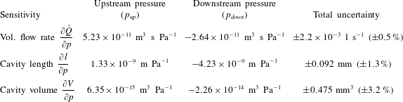
Numerical uncertainties are determined following a grid dependence analysis and a sensitivity analysis. Due to the time consuming nature of the simulations, both analyses have been conducted for the high intensity cavitation number, at $Cn=2.18$ , and the relative errors are assumed to be similar for low cavitation number operation as well.

First of all, a mesh dependence study was conducted to determine the errors arising from the finite discretization. The mesh was coarsened by a factor of 2 everywhere and the conditions of case 2 ( $Cn=2.18$ ) were evaluated to determine the flow rate, cavity length and volume dependence on the mesh resolution. The change between the coarse and fine mesh resolutions may be used to determine the Richardson error estimator at the fine mesh ( $E_{fine}$ ) and the grid convergence index (GCI), following (Roache Reference Roache1997), as shown below:

(3.1)

$$\begin{eqnarray}\displaystyle & \displaystyle E_{fine}=\frac{\unicode[STIX]{x1D700}}{1-r^{k}} & \displaystyle\end{eqnarray}$$

(3.2)

$$\begin{eqnarray}\displaystyle & \displaystyle \text{GCI}_{fine}=F_{s}|E_{fine}|. & \displaystyle\end{eqnarray}$$

In the aforementioned equations, $\unicode[STIX]{x1D700}$ stands for the difference in the observed quantity between fine and coarse meshes, $r$ is the ratio of the fine to coarse mesh spacing (here it is 2), the exponent $k$ represents the formal order of accuracy of the employed method (here equal to 2) and $F_{s}$ is a safety factor, equal to 3 according to the relevant recommendation by Roache (Reference Roache1997).

A complete analysis of the numerical uncertainties should, ideally, include the sensitivity of all simulation parameters (Coleman & Steele Reference Coleman and Steele2009), such as boundary conditions, model coefficients, material properties, etc. However, this would involve an enormous computational effort, given the fact that the discussed simulations are inherently unsteady and need statistical sampling. For this reason it was decided to focus mainly on parameters affecting the simulation for which uncertainty data are available, such as the upstream and downstream pressure boundaries. The influence of the boundary condition input uncertainty was analysed by determining the sensitivity of flow rate, cavity length and cavity volume to the upstream and downstream pressures, for which uncertainties are known. Sensitivities were estimated by shifting pressure conditions at the boundaries by a small amount, equal to 0.5 % of their nominal value (nominal values are reported in table 1).

4 Experimental and numerical results

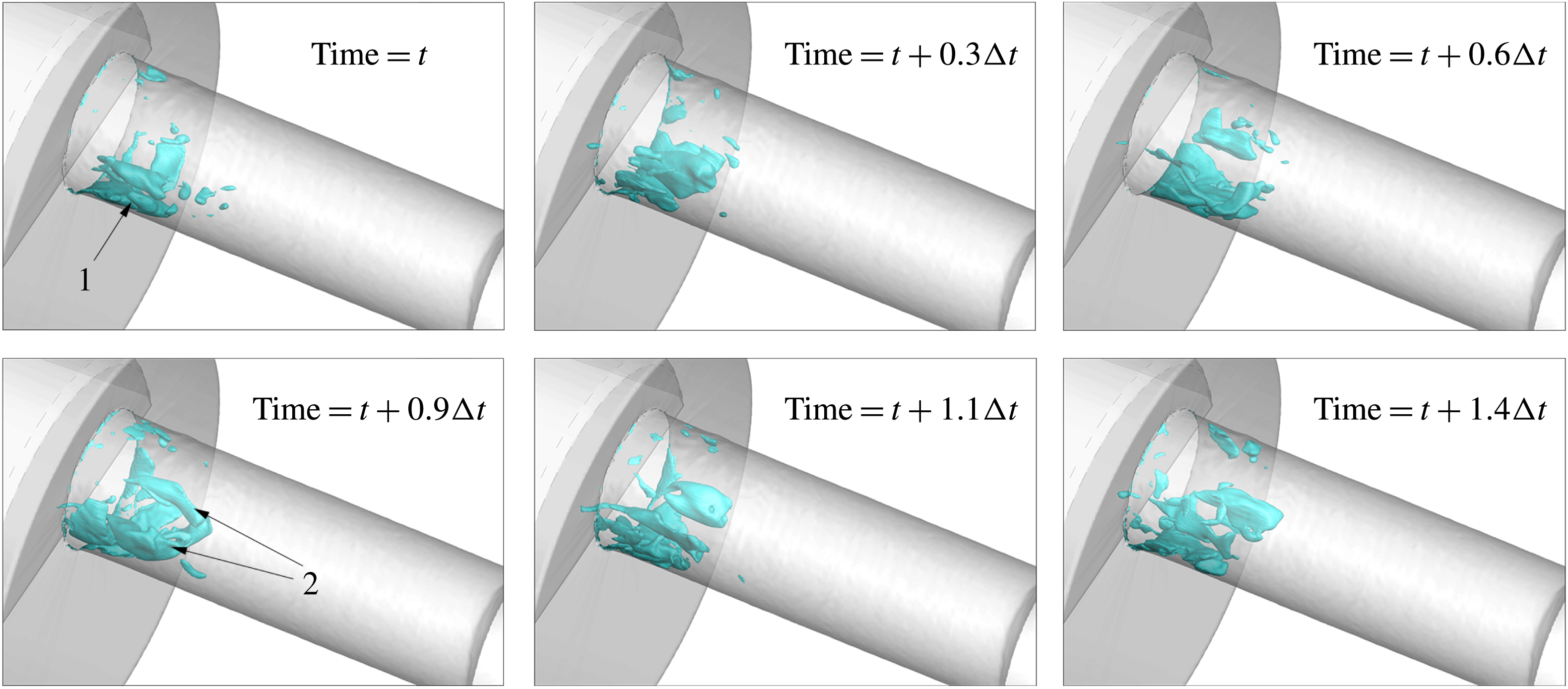
In this section indicative instances mainly of the high cavitation number ( $Cn=2.18$ ) operation will be presented. The reason for this decision is that at low cavitation number ( $Cn=1.5$ ) cavitation is sparse and mainly limited to near the orifice entrance, so relevant shedding phenomena are not that pronounced. Example instances of a 3-D representation of cavitation are shown in figures 5 and 6. The topology of the cavitation pattern may be divided in the following structures: (1) a sheet cavity, formed at the edge of the orifice entrance, oscillating at a Strouhal number of ${\sim}0.35$ –0.38, based on orifice diameter and average flow velocity (attached cavity shedding period of 78– $95~\unicode[STIX]{x03BC}\text{s}$ for high and low cavitation number operation respectively), (2) two large cavitation lobes, which essentially are large cavitating vortices, formed in the core of the orifice and (3) smaller cavitating vortices that occasionally detach from the aforementioned structures and travel downstream of the orifice, or even inside the collector volume (see indicative instances for $Cn=2.18$ , figure 16). At low cavitation number ( $Cn=1.5$ ), it is relatively easy to identify the cavitation structure topology, due to its sparse distribution; in fact, the two cavitating lobes may extend from the needle surface, up to 3 mm downstream the orifice entrance and occasionally may completely disappear, leaving only the attached sheet cavity at the orifice entrance (see the sequence in figure 5). On the other hand, at high cavitation number, the two cavitating lobes persist indefinitely, extending up to 8 mm downstream the orifice entrance, obstructing a large portion of the flow passage and blocking the view to the sheet cavity (see sequence at figure 6). An alternative view of the sheet cavity development is in figure 7, shown as a slice at the midplane of the orifice. In both cases, the location of the cavitating lobes coincides with the position of large counter-rotating vortical structures formed in the cross-section of the orifice (see also figures 8–10).

Figure 5.

Indicative instances of a cavity shedding cycle, shown for $Cn=1.5$ : 50 % liquid isosurface. (1) indicates the attached cavity sheet, (2) the pair of cavitating vortices. Here $\unicode[STIX]{x0394}t$ is the attached cavity shedding cycle period, corresponding to $95~\unicode[STIX]{x03BC}\text{s}$ .

Figure 6.

Indicative instances of a cavity shedding cycle, shown for $Cn=2.18$ : 50 % liquid isosurface. (1) Indicates the attached cavity sheet, (2) the pair of cavitating vortices, which occupy the whole orifice cross-section. Here $\unicode[STIX]{x0394}t$ is the attached cavity shedding cycle period, corresponding to $78~\unicode[STIX]{x03BC}\text{s}$ .

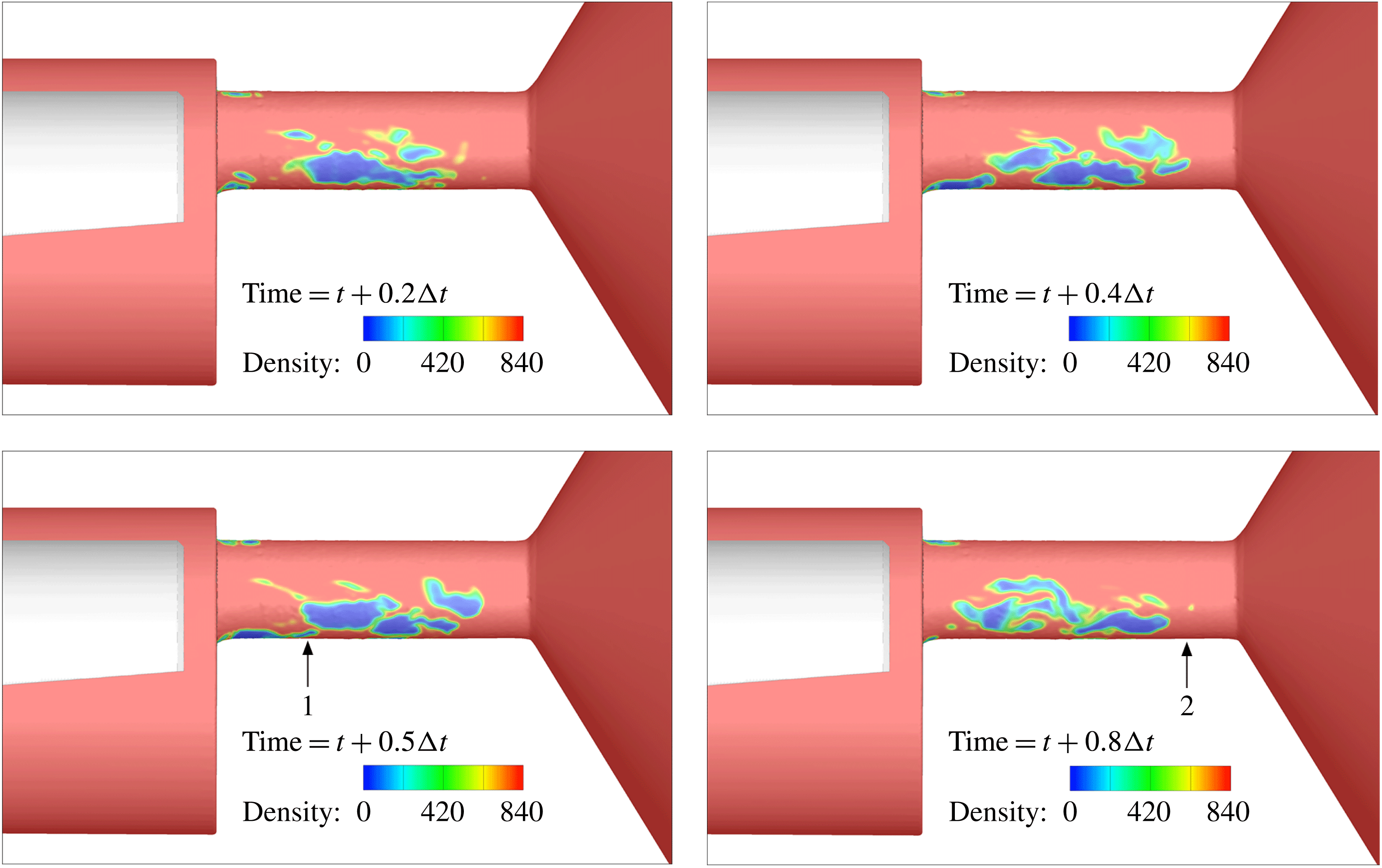
Figure 7 shows the density distribution at the midplane of the geometry for the duration of a cavity shedding cycle, $Cn=2.18$ . This representation was chosen to obtain a view unimpeded by the two cavitation lobes. As is expected, cavitation structures are formed at the side where the majority of the flow enters, i.e. the side that is relatively unobstructed by the throttling needle presence. Examining the orifice side where extended cavitation develops, cavitation structures form at the edge of the orifice entrance and expand further downstream (see the instances at $0.2\unicode[STIX]{x0394}t$ and $0.4\unicode[STIX]{x0394}t$ ). These structures remain attached on the orifice wall and extend up to 2 mm from the entrance. At the trailing edge of these structures, cavities may detach and travel further downstream, dragged by the flow. The sheet cavity growth/collapse cycle is repeated every ${\sim}78~\unicode[STIX]{x03BC}\text{s}$ , corresponding to a Strouhal number ( $St=fL/U$ , where $f$ the shedding frequency, $L$ the orifice diameter, equal to ${\sim}3$ mm and $U$ the characteristic velocity of $100~\text{m}~\text{s}^{-1}$ ) of 0.38. Cavitation structures collapse at different locations; the attached cavity collapses at ${\sim}2$ mm from the orifice entrance, whereas shed cavities collapse at approximately 7–8 mm downstream of the entrance (see also the instances at $0.5\times \unicode[STIX]{x0394}t$ and $0.8\times \unicode[STIX]{x0394}t$ , respectively). The obstructed side of the orifice exhibits cavitation formation, but mainly in the form of attached cavities without significant shedding. This side is also free of erosion, as will be shown later on.

Figure 7.

Indicative instances of a cavity shedding cycle, shown for $Cn=2.18$ . Two collapse sites can be identified at points indicated with (1) and (2). Here $\unicode[STIX]{x0394}t$ is the attached cavity shedding cycle period ( ${\sim}78~\unicode[STIX]{x03BC}\text{s}$ ). The shedding cycle corresponds to a Strouhal number of ${\sim}0.38$ . Density units are $\text{kg}~\text{m}^{-3}$ . The flow moves from left to right.

Figure 8.

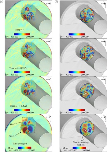
The $z$ -vorticity ( $\unicode[STIX]{x1D714}_{z}$ ) distribution at the cross-section 0.5 mm upstream the entrance (a) and 2 mm downstream the orifice entrance (b), $Cn=1.5$ , for indicative instances and for the time-averaged velocity field. Units are $\text{l}~\text{s}^{-1}$ . Here $\unicode[STIX]{x0394}t$ corresponds to the shedding period, i.e. ${\sim}95~\unicode[STIX]{x03BC}\text{s}$ . The thick white line indicates 50 % liquid volume fraction isoline for instantaneous and 90 % time-averaged liquid volume fraction. The collector volume has been blanked for clarity.

Figure 9.

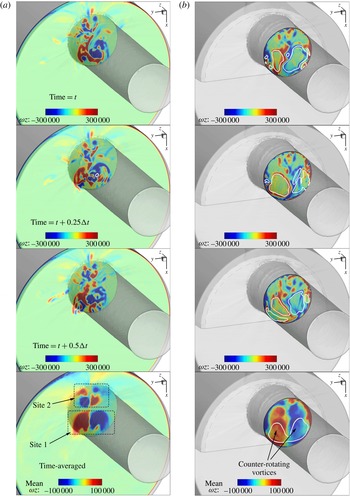
The $z$ -vorticity ( $\unicode[STIX]{x1D714}_{z}$ ) distribution at the cross-section 0.5 mm upstream the entrance (a) and 2.5 mm downstream the orifice entrance (b), $Cn=2.18$ , for indicative instances and for the time-averaged velocity field. Units are $\text{l}~\text{s}^{-1}$ . Here $\unicode[STIX]{x0394}t$ corresponds to the shedding period, i.e. ${\sim}78~\unicode[STIX]{x03BC}\text{s}$ . The thick white line indicates 50 % liquid volume fraction isoline for instantaneous and 75 % time-averaged liquid volume fraction. The collector volume has been blanked for clarity.

Figure 10.

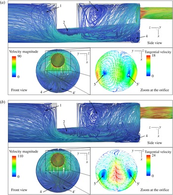
Average flow topology upstream and inside the orifice. Side view and front view streamlines are coloured according to the average velocity magnitude. The zoomed view at the orifice shows a slice (upstream view inside the orifice at 7 mm downstream the entrance) with the average tangential velocity streamlines (coloured according to the tangential, to the slice, velocity magnitude). The numbers indicate vortices, whereas the prime symbol $(\prime )$ indicates symmetric, to the midplane, structures. Results correspond to (a) $Cn=1.5$ , (b) $Cn=2.18$ ; the average flow topology is essentially identical.

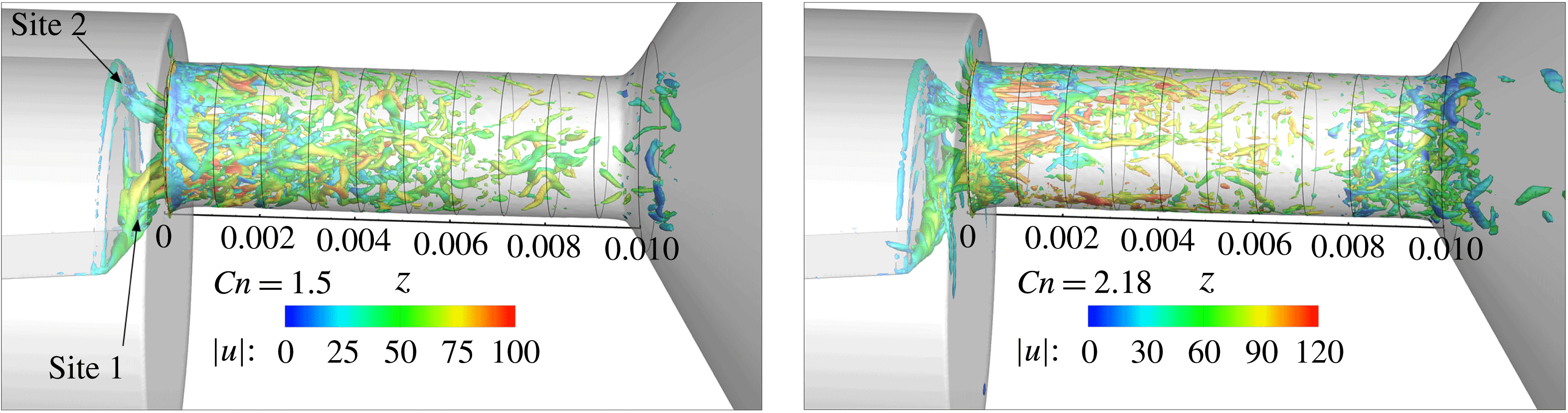
Figures 8 and 9 show the $z$ -vorticity distribution at two indicative slices, one 0.5 mm upstream and one 2–2.5 mm downstream the orifice entrance. Several instances are selected for both low and high cavitation number operation. Despite the highly irregular structure of the instantaneous $z$ -vorticity distribution, some features are clearly observable. First of all, at 0.5 mm upstream the orifice entrance, it is clear that there is an alternating pattern of vorticity sign, indicating counter-rotating vortices. These counter-rotating vortices may be grouped into two distinct sites (‘Site 1’ and ‘Site 2’), note that it is easier to conceive the pattern through the time-averaged velocity field. These sites are associated with the coherent vortical structures shown in figure 12 and cavitation may form there occasionally (see also figure 14 and figure 15). Further downstream of the orifice entrance, $z$ -vorticity distribution is more irregular, although it is still recognizable that the left and right parts of the cross-section are mainly dominated by structures of opposite vorticity sign, i.e. highly transient, large and irregular counter-rotating vortices, which may cavitate, intermittently at low intensity cavitation ( $Cn=1.5$ ) or continuously at high intensity cavitation ( $Cn=2.18$ ).

Another observation is that the vorticity distribution is somewhat more irregular at low cavitation intensity, $Cn=1.5$ , than high cavitation intensity, $Cn=2.18$ . As will be explained later on, this is an effect of turbulence suppression due to the extended cavitation formation at high Cn operation. The averaged flow field vorticity distribution shows clearly the extents of the two counter-rotating vortices occupying the core of the orifice cross-section, also depicted in figure 10, as the time-averaged flow field streamlines. Both operating conditions at $Cn=1.5$ and 2.18 show a similar average flow topology, but flow velocities are slightly higher for the $Cn=2.18$ case. Moving from the inlet and following the flow towards the orifice, the first geometric feature encountered is the needle support structure, which obstructs part of the flow path. The blockage induces flow detachment, which is associated with a longtitudinal horseshoe vortex, indicated with the number 1 in figure 10 (shown only from side view, though the vortex is symmetric and the two parts bridge over the midplane).

The edges of the needle support structure induce a symmetric pair of vortices, indicated with 2 in figure 10, which extend in the expanding fluid region upstream the orifice entrance. The sharp expansion after the needle support causes flow detachment, with the formation of a symmetric pair of vortices at the sides of the needle tip similar to those occurring downstream a backward facing step, denoted with the number 3. Also the direction changes and the strong constriction at the orifice entrance causes flow detachment and the associated vortex tube indicated with number 4 in figure 10. Examining the flow inside the orifice, 7 mm downstream the entrance, a pair of counter-rotating vortices are visible, indicated with the numbers $5$ and $5^{\prime }$ . An observable difference is that at $Cn=1.5$ the average tangential velocity is slightly higher at the circumference of the cross-section, whereas at $Cn=2.18$ the average tangential velocity is higher at the midplane. A slight asymmetry is also observable in the average tangential distribution in both cases; it is speculated that this is related to the asymmetric geometry features of the orifice surface, since such asymmetries were observed in the average cavitation distribution as well.

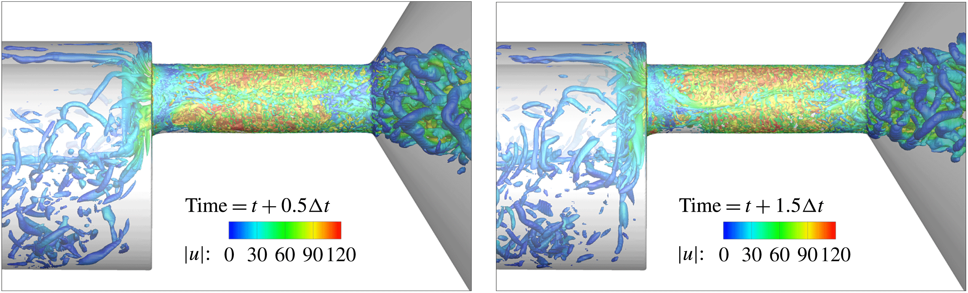
The flow in the simulated section is turbulent; the Reynolds number ranges from 15 000 at the annulus, upstream the orifice, to 100 000, instantaneously, downstream the collector. Figure 11 shows the coherent turbulent structures (i.e. vortices) at the vicinity of the orifice. The turbulent structures are indicated using the second invariant of the velocity gradient tensor, also known as $q$ -criterion (Haller Reference Haller2005; Green, Rowley & Haller Reference Green, Rowley and Haller2007), for a value of $q=10^{9}~\text{s}^{-2}$ . As shown, the flow field is highly transient with velocities reaching $120~\text{m}~\text{s}^{-1}$ . A particular complexity of the flow in this geometry is that turbulent structures are generated upstream the orifice entrance due to the constriction imposed by the support structure of the needle. It was found that these vortices can have a detrimental effect on the flow further downstream. However, due to the low local velocities upstream the orifice, a long simulation time was needed as a transitional stage, for the build up of these structures and their propagation to the orifice entrance. While upstream of the orifice turbulent structures have a relatively random orientation, as the flow moves near the entrance, vortices start to elongate and stretch. The needle flat surface itself acts as a starting point of vortical structures, which extend inside the orifice, in the streamwise direction. As shown in figure 5 and later on, these vortical structures may occasionally cavitate, due to the strong centrifugal forces. The formation of such structures, starting from the needle is a manifestation of Helmholtz’s second theorem (Batchelor Reference Batchelor2000), which states that a vortex tube cannot start or end in a (inviscid) fluid; it must extend to a boundary or form a loop. Additional vortical structures are formed at the region surrounding the high velocity jet expelled in the collector chamber and are the outcome of shear layer instabilities.

Figure 11.

Representation of coherent vortical structures at two indicative instances, employing the $q$ -criterion (using a value of $q=10^{9}~\text{s}^{-2}$ ), at $Cn=2.18$ . The colouring is according to the local velocity magnitude (units are $\text{m}~\text{s}^{-1}$ ). The flow moves from left to right. $\unicode[STIX]{x0394}t$ is the attached cavity shedding period, $78~\unicode[STIX]{x03BC}\text{s}$ .

Figure 12.

Comparison of the turbulent structures between the two operating conditions at $Cn=1.5$ and $Cn=2.18$ in an indicative instance. The isosurface of $q=2\times 10^{10}~\text{s}^{-2}$ is used for the representation, coloured according to the local velocity magnitude (units are $\text{m}~\text{s}^{-1}$ ). The flow moves from left to right.

The instantaneous vortical structures at high and low cavitation number are shown in figure 12; in both cases the same value of $q=2\times 10^{10}~\text{s}^{-2}$ is shown in order to have an objective comparison of structures of the same strength. Note that both are fully turbulent conditions, but $Cn=2.18$ is at a slightly higher Reynolds number ( ${\sim}10\,\%$ higher). For both cases it is clear that there are mainly two agglomerations of vortical structures starting from the needle surface, at regions indicated as ‘Site 1’ and ‘Site 2’ and extending inside the orifice (see also figures 8 and 9). At low cavitation number, $Cn=1.5$ , these are clearly separated and distinct, whereas at high cavitation number, $Cn=2.18$ , they appear fuzzier, entangled and twisted. At low cavitation number vortical structures are mainly concentrated near the orifice entrance and slowly diminish towards the orifice exit, following the flow. On the other hand, at high cavitation number, vortical structures have a clearer streamwise direction near the orifice entrance, whereas they are, in general, sparse in the middle of the orifice due to the presence of cavitation which has the effect of locally suppressing turbulence, see also Gnanaskandan & Krishnan (Reference Gnanaskandan and Krishnan2016). However, there is a concentration of turbulent structures at the area of collapse, i.e. at 7–8 mm downstream of the entrance.

Figure 13.

Comparison of the turbulent kinetic energy averaged at slices across the orifice for the two conditions examined.

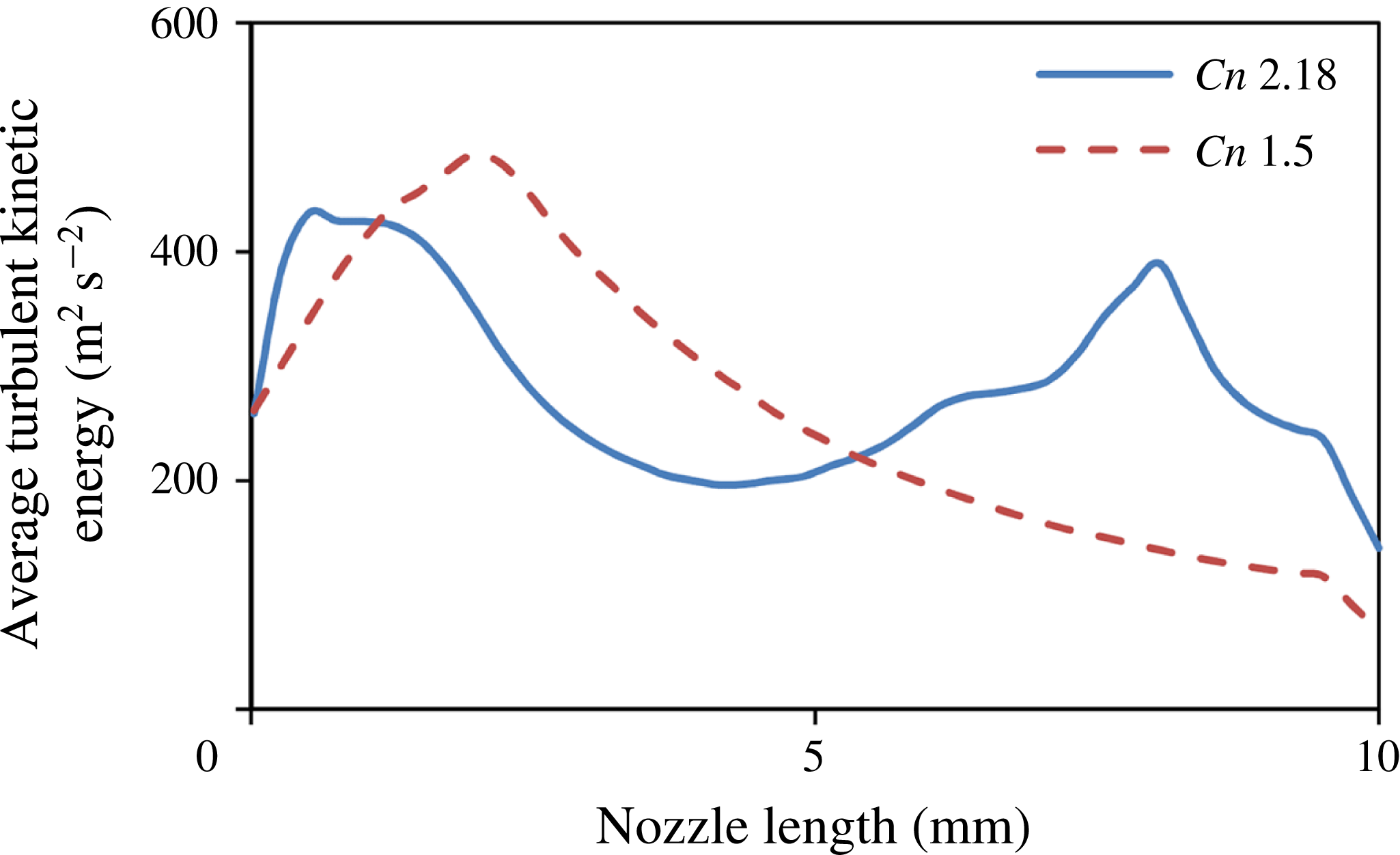
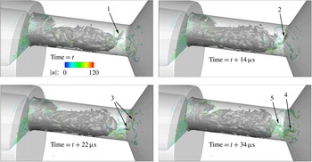
These observations may be represented in a more concise manner, considering the averaged turbulent kinetic energy (containing simulated and modelled/subgrid scales) across the length of the orifice, see figure 13. As described above, operation at $Cn=1.5$ shows a peak of turbulent kinetic energy at ${\sim}2$ mm downstream of the orifice entrance and slowly diminishes afterwards. On the other hand, high cavitation number operation shows two peaks, one at ${\sim}1$ mm downstream of the entrance and another at ${\sim}8$ mm downstream of the entrance. The locations of the turbulent kinetic energy peaks seem to be related with the areas of cavitation collapse in both examined cases. This can be explained by two mechanisms:

(i) turbulence suppression caused by the presence of cavitation. This explains the low values of turbulent kinetic energy near the orifice entrance for low cavitation intensity ( $Cn=1.5$ ) operation and the local minimum from 2 to 8 mm for high cavitation intensity ( $Cn=2.18$ ) operation.
(ii) Cavitation collapse induces a strong disturbance of the flow field; during collapse very high pressures and velocities are generated locally, increasing the turbulent fluctuations in the areas of collapse.

Figure 14.

Indicative images showing the flow features in the vicinity of a cavitating vortex, starting from the needle and moving inside the orifice for high cavitation number ( $Cn=2.18$ ). From left to right: flow streamlines coloured according to velocity magnitude (in $\text{m}~\text{s}^{-1}$ ), isosurface of $q$ -criterion (value $7.5\times 10^{10}~\text{s}^{-2}$ ), coloured according to velocity magnitude and isosurface of the liquid fraction at 95 %. The flow moves from left to right.

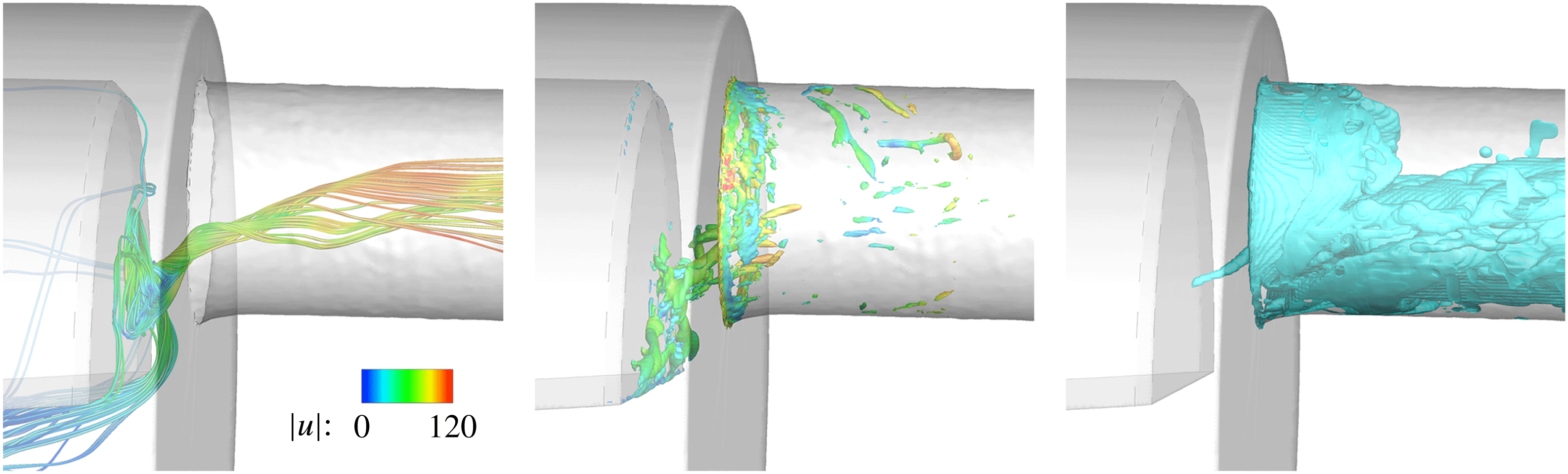
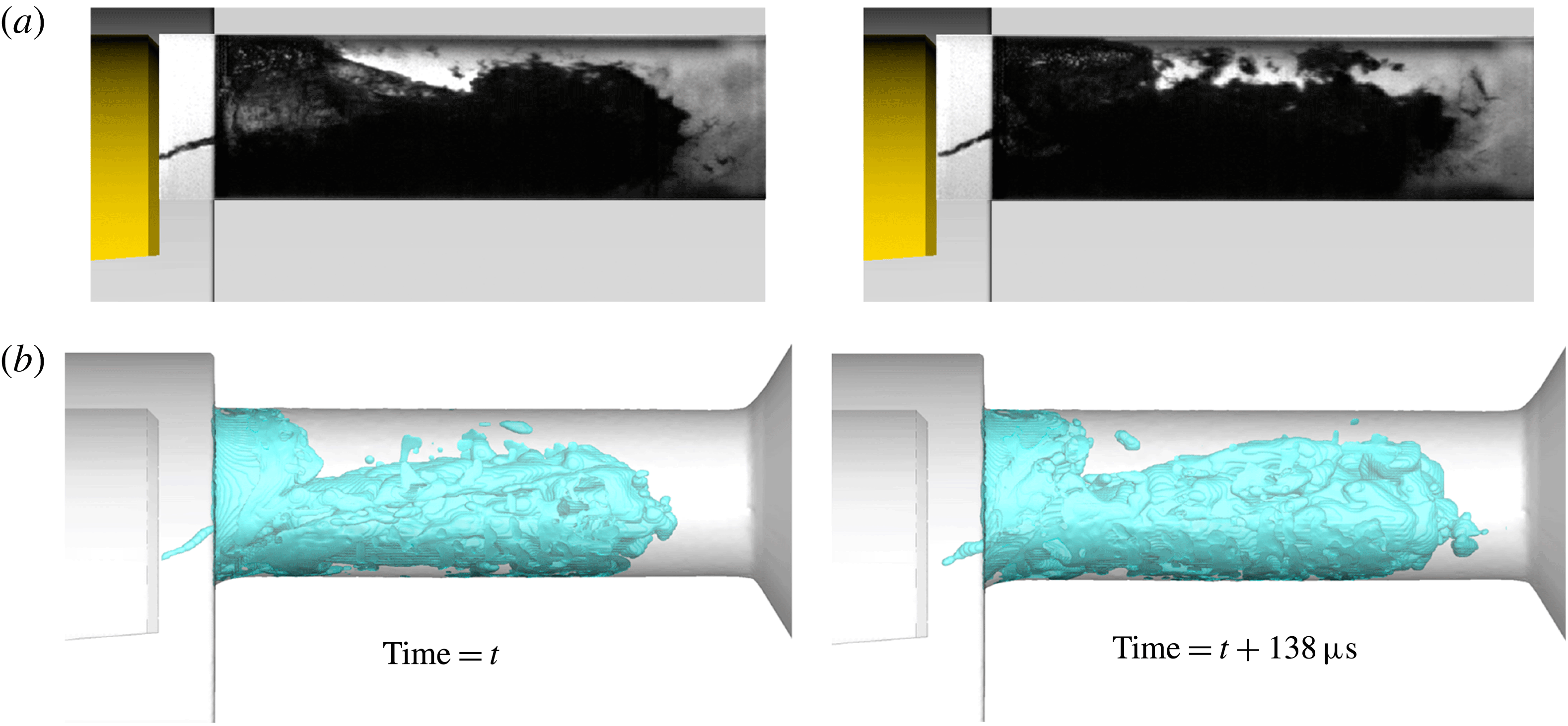
In figures 14 and 15 details of a cavitating vortex, starting from the needle, are shown. The swirling motion of the flow is evident by observing the flow streamlines or by considering the local isosurface of the $q$ -criterion (figure 14). The intensity of the swirling motion is enough to reduce the pressure in the vortex core and trigger the formation of a vaporous cavity that has an elongated shape, following the shape of the corresponding vortex, as visualized with the density isosurface in figure 14. This particular cavitating vortex starts from ‘Site 1’, as was previously discussed, although both sites are prone to cavitating vortex formation. Such effects have been found in the visualization of experiments as well, see figure 15. Even though the vortical fluid motion persists in the local vicinity of the two aforementioned sites, the existence of cavitating vortices is highly unsteady. It is stressed that visualization of a cavitating vortex in figure 15 does not exclude the existence of other, non-cavitating, vortices, since shadowgraphy cannot reveal the presence of the latter. As illustrated in figure 14, the $q$ -criterion representation indicates many vortical structures starting from the needle, only one of which is cavitating at the given instance.

Figure 15.

Indicative instances showing the formation of cavitating vortices, starting from the needle and extending inside the orifice, $Cn=2.18$ . (a) Shadowgraphy from experiment, (b) simulation results, visualized with a liquid fraction isosurface at 95 %. The flow moves from left to right.

Another manifestation of vortical cavities is downstream of the area of the cavity collapse; these correspond to the third topological type of cavities, as discussed. The intensely swirling flow formed downstream of the area of collapse may protect some detached vaporous cavities, allowing them to travel further downstream despite the pressure field recovery. An example of this effect is shown in figure 16, where a vaporous cavity is able to reach the exit of the orifice and enter the collector volume. Note that the collector pressure is approximately 17 bar. In the indicative instances provided, a cavity is detaching (1), then it elongates, following the stretching of the vortex (2), later on breaks (3) and eventually collapses (4). At the end of the process, another cavity detaches (5).

Figure 16.

Cavitating vortices are formed at the trailing edge of the cavity inside the orifice, high cavitation number operation ( $Cn=2.18$ ). Cavitation structures (75 % liquid) are shown as a black/dark grey isosurface for contrast, whereas the semi-translucent isosurface represents vortex cores ( $q=5\times 10^{10}~\text{s}^{-2}$ , coloured according to velocity magnitude); as visible, detached cavitation structures may be associated with relevant vortex cores. The flow moves from left to right.

The average flow rate through the orifice is shown in table 5. As shown, the maximum error is 1.3 %, at the highest cavitation number, which is close to the validation uncertainty of ${\sim}0.8{-}0.9\,\%$ .

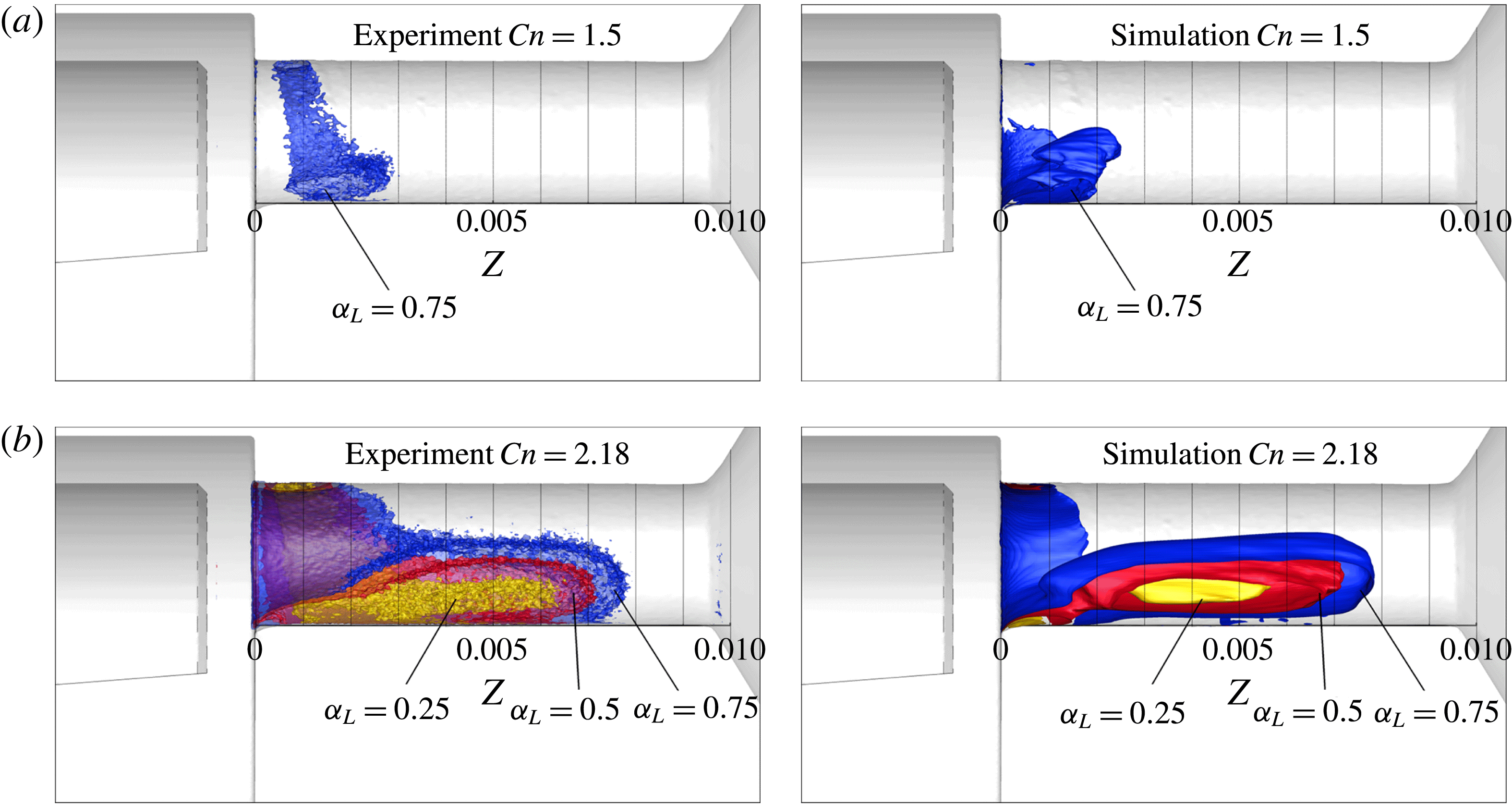
At low cavitation number ( $Cn=1.5$ ), the average amount of vapour is low and mainly located near the entrance of the orifice. The average cavitation extent from the CT measurements spans from 0.5 mm to ${\sim}2.8$ mm downstream of the orifice entrance, estimated using an isosurface of 75 % liquid fraction; lower liquid fractions cover much smaller areas and are more noisy. Simulation results indicate that cavitation starts from the entrance of the orifice and reaches 2.5 mm downstream, for the same liquid fraction isosurface (75 %). The picture is substantially different at the high cavitation number case examined, at $Cn=2.18$ , where cavitation spans from the orifice entrance and covers 80 % of its length. The experimental results indicate that the isosurfaces of 25 %, 50 % and 75 % liquid reach ${\sim}6$ , 7 and 8 mm, respectively. Simulation results indicate the same pattern as well, with the isosurface of 25 % liquid slightly less extended. It is notable that both numerical simulation and experiment show that the isosurface of 25 % liquid is detached from the wall. An indicative averaged liquid fraction distribution is shown in figure 17 at low and high cavitation number, $Cn=1.5$ and 2.18, for both the experiment and simulations. Differences in the average cavity length are within the validation uncertainty ( ${\sim}0.1$ mm) for the 50 % average liquid isosurface at $Cn=2.18$ .

Figure 17.

Side view of the orifice, showing average liquid fraction isosurfaces ( $a_{L}=0.25$ , 0.5 and 0.75 represented with yellow, red and blue colours respectively) for $Cn=1.5$ (a), $Cn=2.18$ (b). Isosurfaces are clipped by the midplane, to show liquid distribution extents with clarity. Black vertical lines are placed every 1 mm, starting from the orifice entrance. The flow moves from left to right.

Figure 18.

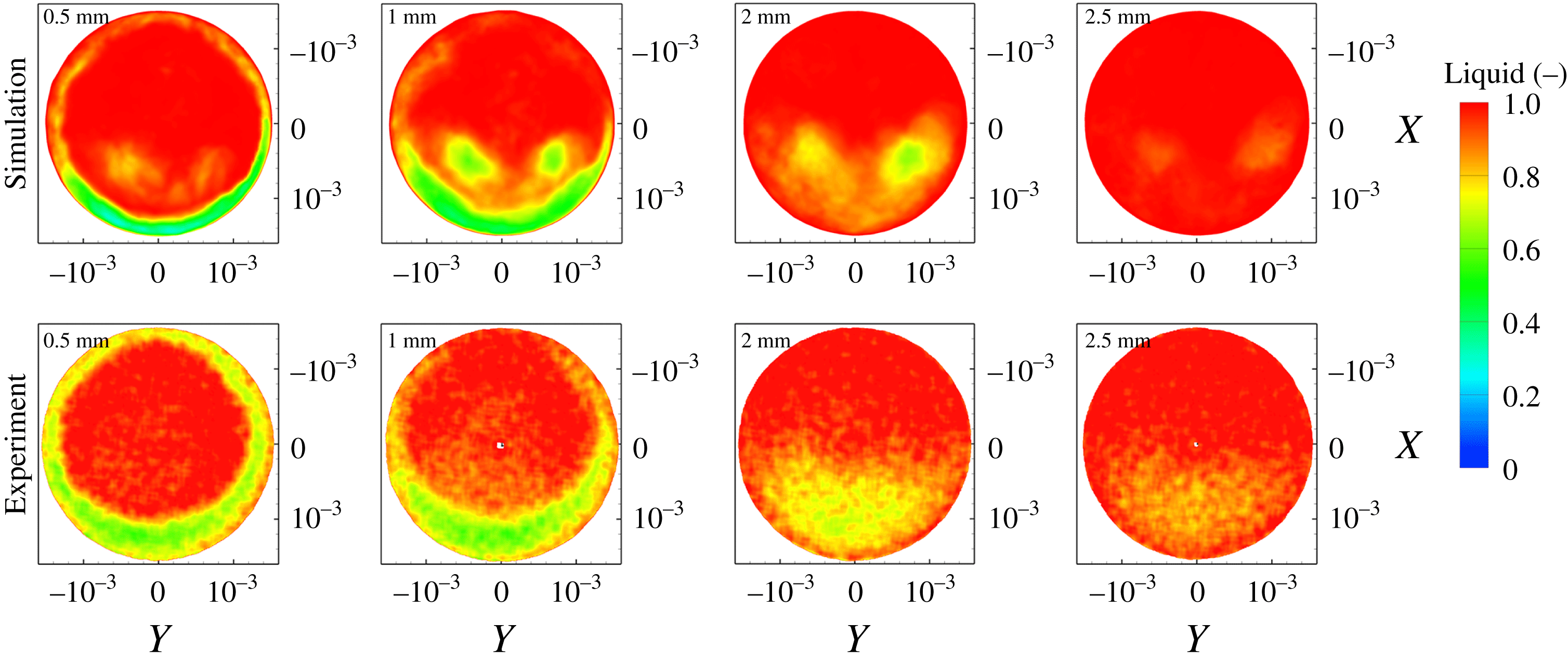
Average liquid fraction distribution at the orifice cross-section for various locations, for $Cn=1.5$ , simulation and experiment (micro-CT) density measurement. The number at the upper left corner indicates the distance from the orifice entrance. Upstream view inside the orifice ( $AA^{\prime }$ view, see figure 4, $A$ being at the top and $A^{\prime }$ at the bottom).

Figure 19.

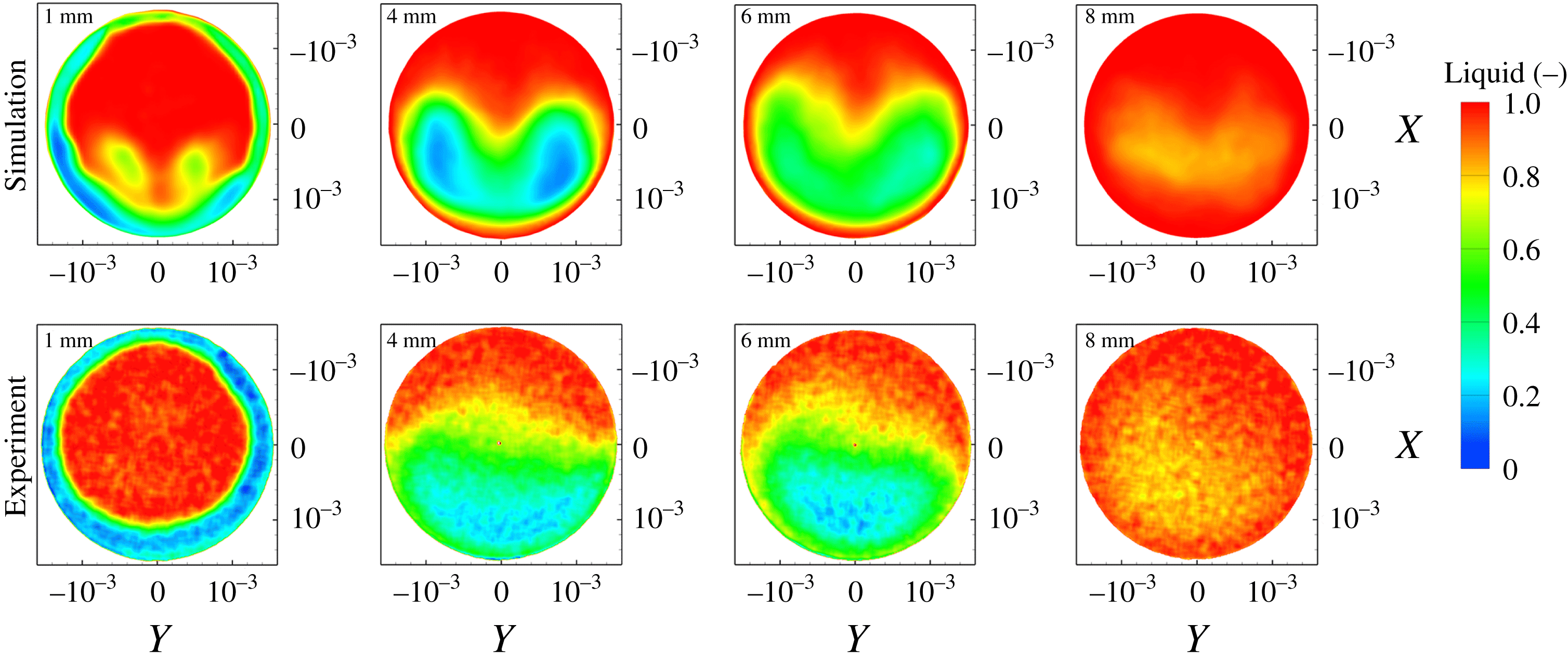
Average liquid fraction distribution at the orifice cross-section for various locations, for $Cn=2.18$ , simulation and experiment (micro-CT) density measurement. The number at the upper left corner indicates the distance from the orifice entrance. Upstream view inside the orifice ( $AA^{\prime }$ view, see figure 4, $A$ being at the top and $A^{\prime }$ at the bottom).

Figure 20.

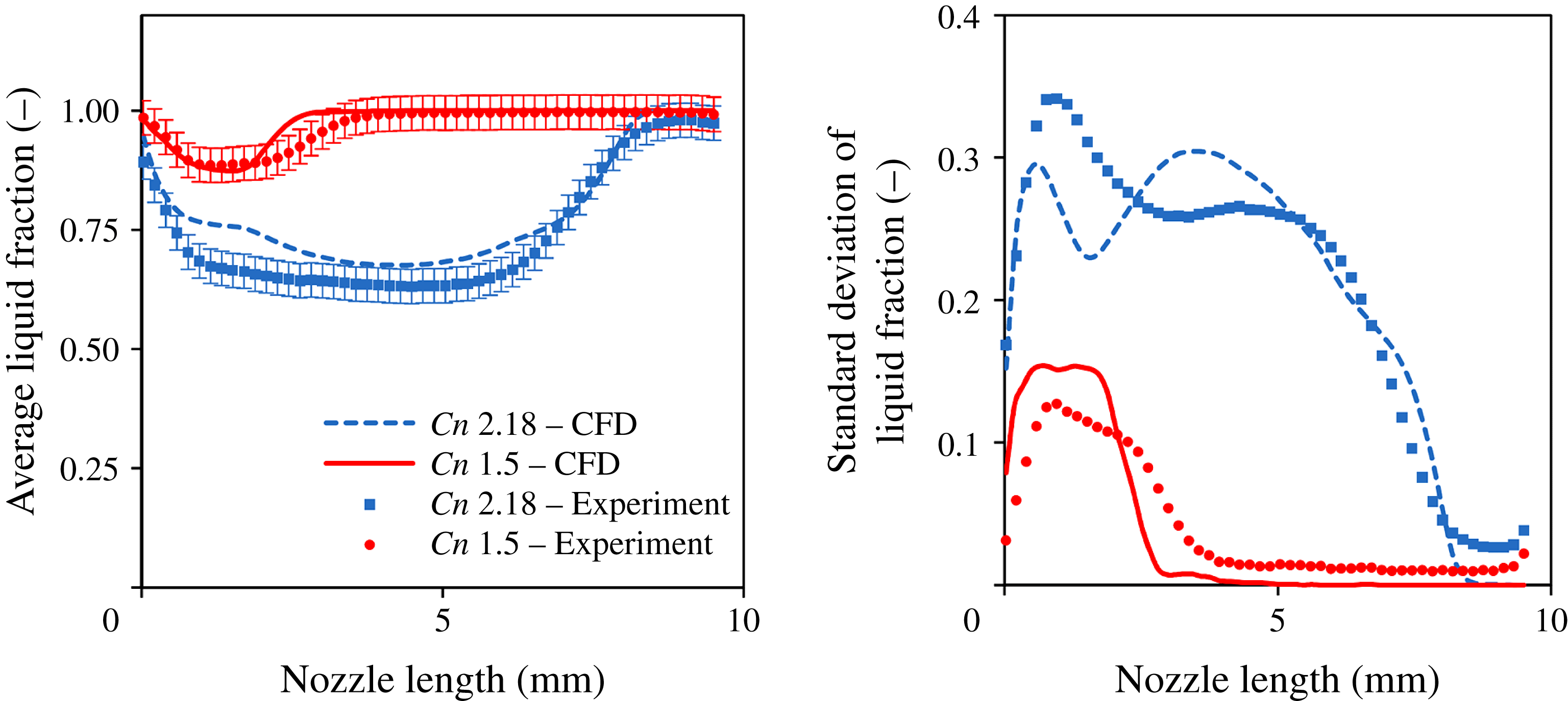
Average and standard deviation of liquid fraction at slices across the orifice length.

Figures 18 and 19 show the average liquid fraction in slices across the length of the orifice for high and low cavitation numbers, based on numerical and experimental data. In general, the average cavitation pattern in both cases shows similar features. Near the orifice entrance there is an attached vapour sheet, while further downstream there is a detached structure. It has to be kept in mind that slices from the CT scans show an artefact at the centre of the orifice, due to the reconstruction algorithm employed; this has been omitted from visualization, hence the white dot appearing at the origin. The experiment shows a more distinct cavitation ring around the entrance of the orifice, both at high and low cavitation number operation. At low cavitation number, the average vapour cavity predicted by the simulation shows two distinct cavitation lobes, with diffuse vapour between them. In the experiment, the two cavitation lobes are not clearly visible, although the left part of the cross-section shows a higher vapour content than the right; this is something found in the simulation results as well (see figure 18 at 1 mm). Simulation results at high cavitation number still show the two distinct lobes (see figure 19 at 1 mm), although the two lobes quickly merge, forming an agglomeration (see figure 19, from 4 mm and further downstream). Experimental results show a more disperse and noisy cavitation distribution, though the general pattern and extent agrees with the simulation. Note that at high cavitation number, as well, the left part of the cross-section shows a higher occupation by cavitation (see e.g. figure 19 at 4 or 6 mm). Cavitation distribution is not entirely symmetric, due to the geometric features of the orifice geometry used, while the asymmetry is lower at the highest cavitation number operation ( $Cn=2.18$ ). The two vapour lobe locations predicted by the simulation coincide with the counter-rotating vortices of the average flow field (see also figure 10), occurring inside the orifice.

Table 3.

Error estimator and grid convergence index (GCI) for case 2, $Cn=2.18$ . The cavity length is estimated using the 50 % average liquid fraction isosurface. Cavity volume is based on the volume integral of the time-average vapour fraction. Both the Error estimator and GCI are expressed at fine mesh level and percentages are expressed in reference to fine mesh solution.

To make a clearer comparison between the simulation and the experimental distribution of the liquid fraction, results of the average and standard deviation distributions of the liquid fraction at slices across the length of the orifice are shown in figure 20. The average liquid fraction expresses the blockage of the flow by cavitation, whereas the standard deviation shows the dispersion of vaporous structures across the cross-section of the orifice. At low cavitation number, simulation results show a slight underprediction of the vaporous cavity length, although minimum liquid fraction is correctly predicted at ${\sim}88\,\%$ . Still, the numerical results are within the validation uncertainty, which is ${\sim}\pm 7\,\%$ , including experimental errors ( ${\sim}\pm 4\,\%$ ) and numerical uncertainty as determined from the sensitivity analysis and grid dependence on average cavity volume (tables 3 and 4). The standard deviation of the liquid fraction shows a peak at 1 mm downstream of the entrance of the orifice, while the simulation predicts a slightly higher standard deviation. Moving further downstream of the cavitation region, the standard deviation drops rapidly. It has to be highlighted that simulation predicts a standard deviation very close to zero from 5 mm downstream of the entrance until the orifice exit, whereas in the experiment there is a non-zero standard deviation of liquid fraction until the orifice exit; this is an indication of noise from the micro-CT 3-D reconstruction of cavitation. On the other hand, simulation tends to overpredict slightly the average liquid volume fraction at high cavitation number, while predicting the correct average cavity length. The mismatch is mainly pronounced at 1.4 mm downstream the orifice entrance. Still, the minimum liquid volume fraction is predicted within the validation uncertainty. The minimum liquid fraction predicted by the simulation is 67 % whereas in the experiment it is found to be 63 %. Both experimental and numerical results of the standard deviation of liquid fraction at the cross-section of the orifice show two peaks, one at ${\sim}0.7$ mm and one at ${\sim}4$ mm downstream of the entrance. The simulation, however, underpredicts the first peak, whereas it overpredicts the other. The shape of the standard deviation variation at the cavity closure is in a close agreement with the experiment.

Table 4.

Uncertainty determination based on sensitivities of volume flow rate ( $\dot{Q}$ ), cavity length ( $l$ ) and cavity volume ( $V$ ) to upstream and downstream pressures. Uncertainty values inside parentheses are relative in respect to reference flow rate ( $0.466~\text{l}~\text{s}^{-1}$ ), cavity length (7.2 mm, corresponding to the 50 % average liquid isosurface) and cavity volume ( $14.7~\text{mm}^{3}$ ).

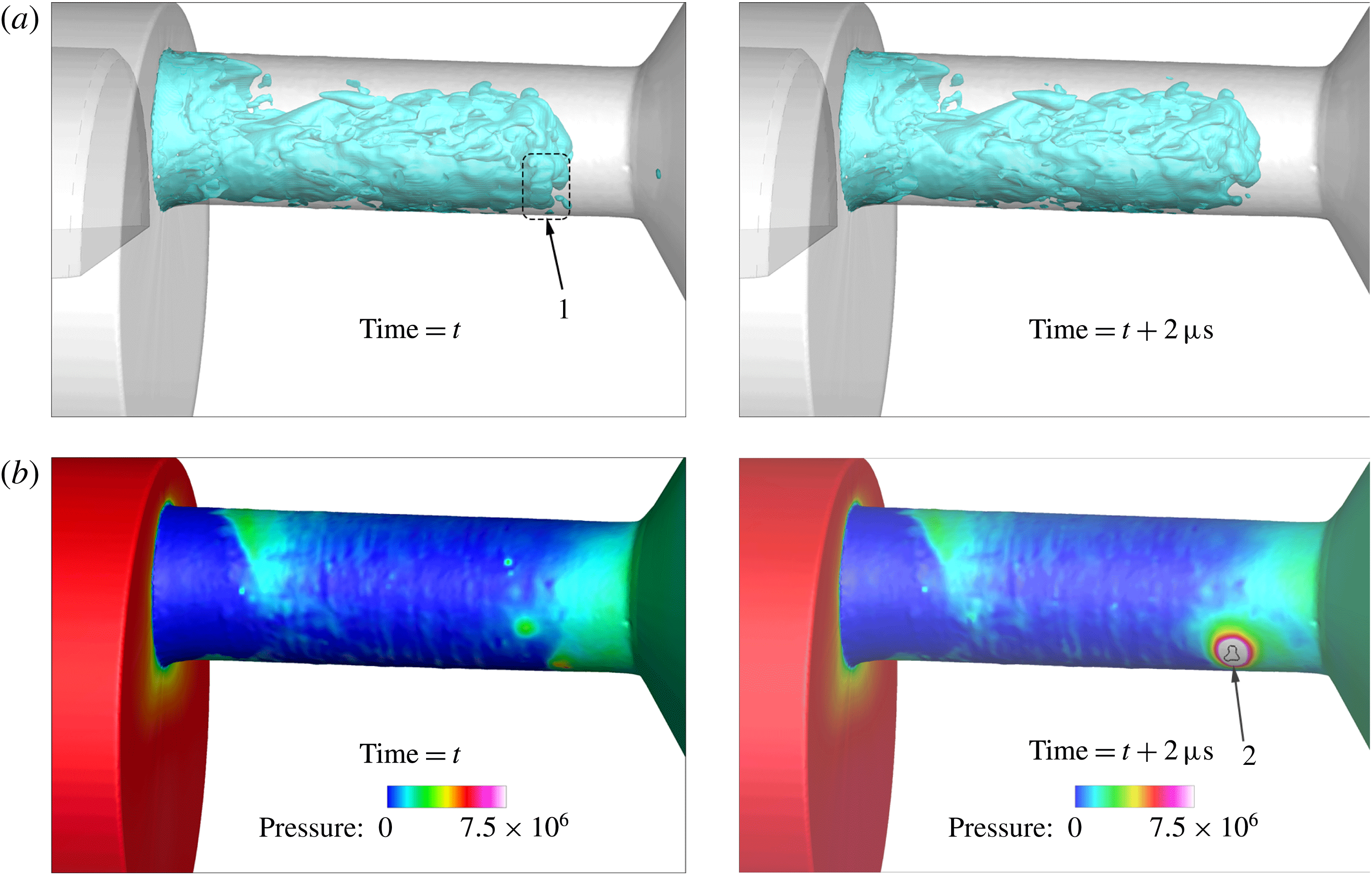
CT scans of the described configuration indicated that, over time, the orifice geometry was changing; it was apparent that exposure to cavitation caused erosion of the material. The simulation with the proposed cavitation model can shed light in the formation of erosion. Indeed, the collapse of arbitrarily shaped vaporous structures can be tracked by the proposed cavitation model, since it predicts very high pressures at the areas of collapse. Indicative flow instances from the simulation are provided below in figure 21 for $Cn=2.18$ , showing density isosurface inside the orifice and the pressure field on the wall. In the instances provided, the collapse of a cavitation structure at the trailing edge of the cavitation cloud is visible, see 1. This collapse induces a very high pressure to the nearby wall surface, see 2. The violence and intensity of the collapse may be understood by considering that pressure, locally, rises from vapour pressure ( ${\sim}0.172$ bar) to 200 bar within $2~\unicode[STIX]{x03BC}\text{s}$ . The location of such high-pressure peaks can provide information on the erosion-prone areas, for more information see also Mihatsch, Schmidt & Adams (Reference Mihatsch, Schmidt and Adams2015).

Table 5.

Volumetric flow rate comparison for the two examined cases. Validation uncertainty for case 1 is based on the same absolute values of uncertainties as case 2.

Figure 21.

Indicative instances of the cavitating flow, at $Cn=2.18$ ( $p_{up}=55$ bar, $p_{down}=17.4$ bar). (a) Density isosurface (75 % liquid), (b) pressure on the wall. Flow is moving from left to right. Notice the cavitation structure marked with (1), which, due to its collapse, causes a pressure pulse on the wall at (2). The collapse occurs within 2 s. Pressure in the area enclosed within the black line in (2) rises to more than 200 bar. Pressure units are Pascal.

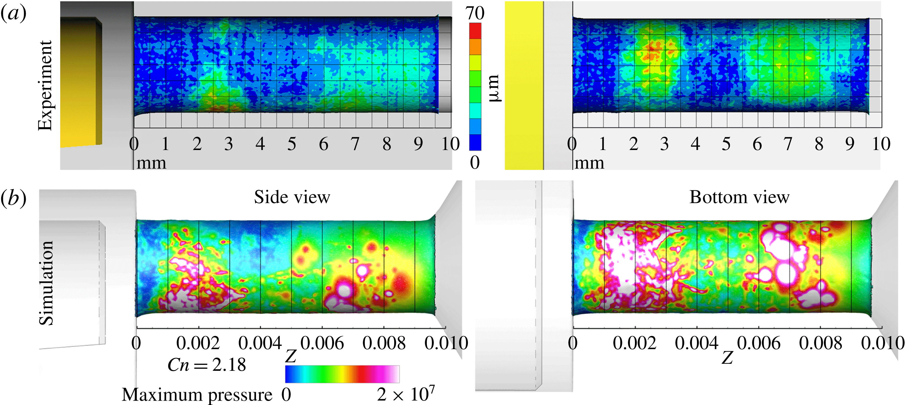
Erosion-prone areas have been identified through the difference of the orifice surface before and after exposure to cavitation. Indicative results are shown in figure 22(a). Erosion develops in two distinct zones, at the orifice sides exposed to cavitation: the first zone spans from ${\sim}1.4$ mm until 3.7 mm downstream of the entrance and the second zone from ${\sim}5.4$ mm until 8.8 mm downstream of the entrance. Undeniably, at low cavitation number conditions, cavitation is limited to near the orifice entrance, thus it is certain that the far downstream erosion site is caused during the high cavitation number operation.

Figure 22.

(a) Erosion location as determined from CT scans of the geometry, expressed as the difference of the orifice geometry prior and after exposure to cavitation. (b) Accumulated maximum of pressure (i.e. pressure peaks) over time on the wall surface for $Cn=2.18$ , simulation results. Pressure units are Pascal. See also supplementary material for a 3-D distribution of pressure peaks around the orifice.

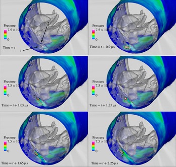
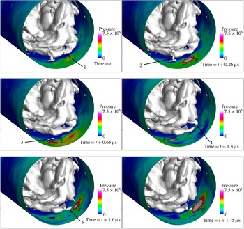
Numerical simulation can provide insight into the erosion development, by recording areas of high pressures caused by the collapse of vapour structures, as illustrated in figures 21, 23 and 24. Indeed, the accumulated local maximum of the instantaneous pressure field at every computational cell shows a distinct pattern which can be well correlated with figure 22(a). At low cavitation number, high-pressure peaks are detected close to the orifice entrance, starting at ${\sim}1$ mm until ${\sim}2.5$ mm downstream of the entrance. At high cavitation numbers, see figure 22(b), the high-pressure peaks are clustered into two zones, one from ${\sim}1$ mm until ${\sim}3.5$ mm and another from ${\sim}5.5$ mm until ${\sim}8.5$ mm downstream of the entrance. These two zones are associated with the collapse locations of the attached cavity and cavity shedding, as shown in figure 7, and show a correlation to the average turbulent kinetic energy distribution, shown in figure 13.

Figure 23.

Instances of collapsing cavitation structures, denoted with the isosurface of the vapour fraction at 75 % liquid (semi-translucent grey/white), with the corresponding pressure field on the wall. Collapsing structures are indicated by an arrow and the resulting pressure pulse with a dashed line. Upstream view inside the orifice ( $AA^{\prime }$ view, see figure 4) at 3.5 mm from the orifice entrance. The rest of the orifice and collector volume have been blanked to provide an unobstructed view to the collapse process. Units are in SI (pressure in Pa).

Figure 24.

Instances of collapsing cavitation structures, denoted with the isosurface of the vapour fraction at 75 % liquid (grey/white), with the corresponding pressure field on the wall. Collapsing structures are indicated by an arrow and the resulting pressure pulse with a dashed line. Upstream view inside the orifice ( $AA^{\prime }$ view, see figure 4) at 9 mm from the entrance. The collector volume has been blanked to provide an unobstructed view to the collapse process. Units are in SI (pressure in Pa).

The pressure peaks indicated with a white colour in figure 22(b) are of pressure levels equal to or higher than 200 bar, which is higher or equal to ${\sim}20\,\%$ of the nominal yield stress of the PEEK material used. Higher magnitude pressure ( ${>}500$ bar) peaks are concentrated mainly at ${\sim}2$ mm and ${\sim}7$ mm downstream of the entrance; note that wall pressure may locally reach 750 bar and pressure inside the liquid bulk may reach 1850 bar. The fact that the predicted wall pressures are lower than the nominal yield stress does not necessarily mean a weakness of the described model; the fatigue failure stress may drop significantly for large numbers of loading cycles (Budynas & Nisbett Reference Budynas and Nisbett2011). As mentioned before, an indicative cavity shedding time scale is ${\sim}78{-}95~\unicode[STIX]{x03BC}\text{s}$ ; considering that erosion was observed over the course of 44 h testing, the number of loading cycles is of the order of $10^{9}$ . At such numbers of loading cycles the material yield stress may drop by more than 50 % compared to nominal. Also, since the smallest vapour scale cannot be smaller than the cell size, the peak pressure is affected by the spatial and temporal resolutions; however, the location of the pressure peaks can provide an indication of erosion sites. For more information the interested reader is referred to Schmidt et al. (Reference Schmidt, Mihatsch, Thalhamer, Adams, Kim, Chahine, Franc and Karimi2014) and Mihatsch et al. (Reference Mihatsch, Schmidt and Adams2015).

A more detailed view of the collapse mechanism appearing in the two erosion sites is provided in figures 23 and 24. As shown in figure 23, the mechanism behind the erosion close to the entrance (the one indicated in figure 22, starting from 1 to 3.5 mm) is the collapse of the attached sheet cavities. Such attached cavities may be disperse and small in size, as e.g. indicated with number 1, producing at their collapse a single pressure pulse. Pressure pulses are also found from the collapse of larger attached cavitation sheets, as indicated with number 2; in that case a series of pressure pulses are produced at the edge of the receding sheet cavity, as indicated by the dashed regions denoted with the number $2^{\prime }$ . On the other hand, the mechanism of erosion at the region towards the exit of the orifice (the one indicated in figure 22, starting from 5.5 to 8.5 mm) is mainly the collapse of detached cavities. As shown in figure 24, both small-scale (indicated with numbers 1, 2) and large-scale (indicated with numbers 4, 5) cavitation structures cause pressure peaks in the nearby walls, albeit the large scales produce higher magnitudes. Apart from detached cavities, there is evidence that small cavity pockets, formed at roughness elements of the wall, may collapse causing local high pressures as well, see 3 in figure 24. At both erosion sites, cavity collapses may be either individual (i.e. a single cavity collapse) or in the form of a ‘collapse cascade’, where a number of collapses is observed in rapid succession. Examples of such ‘collapse cascades’ are e.g. the receding of the cavity sheet at 2 in the sequence of figure 23 and collapses 4 and 5 in the sequence of figure 24.

An alternative way of depicting the collapse distribution of cavitation structures is through the volume representation of the collapse epicentres. The distribution of the collapses is shown in figure 25 as a side view (similar to figure 22) and along the orifice cross-section. Pressure peaks located near the orifice entrance (0–5 mm downstream the entrance, first erosion site when moving with the flow) are mainly concentrated very close to the walls, indicating the collapse of attached cavities. On the other hand, collapse epicentres are much more scattered all across the orifice cross-section at the second collapse site (5–10 mm downstream of the throttle entrance), indicating the collapse of detached cavities that travel in the bulk of the fluid.

Figure 25.

Collapse epicentres for $Cn=2.18$ , marked as scatter plot (spheres) inside the volume of the orifice; only collapse pressures equal or higher to 200 bar are shown. The size of the spheres is proportional to the pressure peak magnitude. Note that in the region between 0–5 mm downstream the entrance, collapse epicentres are very close to walls, whereas between 5–10 mm collapse epicentres are scattered all across the cross-section of the orifice.

5 Discussion

The examined cases illustrate the complexity of the flow in a relatively simple configuration that has both industrial and scientific interest due to the wealth of flow features that are occurring. The off-centred orifice geometry causes the formation of an asymmetric cavitation pattern and cavitating vortices, that are similar to those occurring in actual diesel injection systems. An important parameter, that affects all micro-fluidic devices, is the accuracy of the geometry representation. Unfortunately manufacturing constraints impose limits to the fidelity of the geometry. On the other hand, precise geometry representation is crucial for capturing accurately the involved flow phenomena. Early experimental and numerical investigations indicated that the flow rate through the cylindrical orifice (idealized geometry) was considerably lower than the actual orifice geometry, due to the presence of sharp corners at the orifice entrance.

The main features of the cavitation structure are: (1) attached cavitation sheets around the orifice entrance, (2) a pair of large counter-rotating cavitating vortices inside the orifice, which may extend up to the needle and (3) cavitation structures that detach from the aforementioned structures and travel downstream. The flow inside the orifice shows strong turbulent characteristics in the form of highly unstable coherent vortical patterns. All these turbulent features are closely related to cavitation formation. The cores of large-scale vortices may act as cavitation nucleation regions, enabling the transient formation and propagation of cavitation structures in areas where time-averaged pressure may be well above vapour pressure. Examples of such cases are the formation of cavitating vortices, starting from the needle of the examined device, or the shedding of cavities inside the collector volume. Another example is shown in figure 26, with the isosurface of the time-averaged pressure distribution at a pressure level equal to the vapour pressure. The region with time-averaged pressure less or equal to the vapour is very limited and located near the entrance of the orifice, with no resemblance to the time-averaged liquid fraction distribution shown in figure 17.

Figure 26.

Time-averaged pressure field at the midplane of the geometry for low and high cavitation numbers. The black isosurface denotes the area where time-averaged pressure is less than or equal to vapour pressure; for $Cn=1.5$ it is barely visible. Pressure units are Pa. The flow moves from right to left.

Flow visualization of the experiment clearly shows unsteady flow features, but only in a qualitative manner. Moreover, only a fraction of these features is visible, due to the optical blockage of the passage from cavitation presence. X-ray micro-CT enabled a quantitative description of the flow field, giving volumetric density distribution and erosion information. The discussed numerical methodology with the proposed cavitation model and the DES turbulence model, is capable of predicting accurately many of the flow features, including cavitating vortices, providing information on the highly turbulent flow field and explaining the erosion formation by tracking the collapse of vaporous structures.

Minor discrepancies are observed at the cavity length mainly at low cavitation number. Reasons for the discrepancies are as follows.

(i) At low cavitation number, cavitation effects are much more sensitive to small variations of the flow rate. Moreover, cavitation is more sensitive to the existence of turbulent structures that have not been resolved with the numerical resolution employed; as the turbulent model used in the present study is a RANS/LES hybrid, the computational mesh employed was not intended to resolve all turbulent structures, not to mention that such an effort would involve an immensely higher computational cost.
(ii) Not all wall features were resolved; inherently, due to the discretization procedure, any wall features below the discretization resolution have been smoothed out. Moreover, erosion development in the experiment alters wall features over time.
(iii) Furthermore, parts upstream the annular passage (i.e. the flow splitting into three inlet pipes and funnel shape contraction) have been excluded, though such geometric features may induce additional turbulence at the inlet of the orifice, e.g. pipe bends are known to introduce streamwise vortices (Tunstall & Harvey Reference Tunstall and Harvey1968).
(iv) Diesel properties were obtained from a property library, however they do not necessarily correspond to exactly the actual diesel properties in the experiment. Diesel fuel samples from different sources have slightly different composition and properties. Moreover, even though diesel fuel was periodically replaced to maintain its quality, the fuel properties do not remain constant after exposure to cavitation, see also Lockett & Jeshani (Reference Lockett and Jeshani2013). As observed in the aforementioned experimental investigation, diesel colour changed towards a more yellowish hue after exposure to cavitation, indicating slight changes in its composition.
(v) The experimental errors should not be considered negligible; as indicated in figure 20, errors in average volume fraction are ${\sim}\pm 0.04$ . Moreover, noise is visible in the average liquid fraction isosurfaces and artefacts in the liquid fraction distribution due to the 3-D reconstruction can be identified (Mitroglou et al. Reference Mitroglou, Lorenzi, Santini, Gavaises and Assanis2015). In total, the discrepancies between numerical and experimental results are within or very close to the validation uncertainty margin, both for flow rate and average cavity volume (and liquid volume fraction).

6 Conclusion

In the present work the cavitating flow inside an orifice was analysed with experimental techniques and numerical tools at low and high cavitation numbers. Shadowgraphy shows cavitation features, like cavitating vortices extending to the needle surface, but optical access inside the orifice is limited due to view blockage by cavitation. X-ray micro-CT scans on the other hand, can provide quantitative information on the average cavitation distribution inside the orifice.

Numerical simulations were used to predict unsteady features of the flow, vapour collapse locations and to derive the average distribution of the liquid fraction. Three types of cavitation structures have been identified, namely attached cavitation at the orifice entrance, large-scale cavitating vortices spanning from the needle and extending inside the orifice and smaller detached cavities travelling further downstream. The flow field is turbulent in the whole test section, however turbulence in the orifice region is affected by cavitation structures. Turbulence is dampened in areas of dense cavitation, whereas it is found to increase in areas of cavitation collapse. The increase in flow turbulence in areas of cavitation collapse is related to the absence of the turbulence damping mechanism and to the very high velocities and pressures induced by the collapse of cavitation structures.

At high pressure locations, which indicate areas of vapour collapse, average liquid fraction distribution and average volumetric flow rate through the orifice were used to validate the results of the numerical simulation. Examination of the flow field in the vicinity of these erosion sites indicates that the one located near the orifice entrance is caused by the collapse of attached cavity sheets, whereas the other, towards the orifice exit, is caused by the collapse of detached cavities. The agreement between simulation and experiment, in all aforementioned items, is within validation uncertainty, taking into account all uncertainties, numerical and experimental. Thus, despite the inherent complexities of the particular flow, a reasonable reproduction of the flow pattern was obtained, close or within the uncertainty margin.

Acknowledgements

The research leading to these results has received funding from the People Programme (IAPP Marie Curie Actions) of the European Union’s Seventh Framework Programme FP7/2007-2013/ under REA grant agreement nos 300410 and 324313. The authors would like also to acknowledge the contribution of The Lloyd’s Register Foundation. Lloyd’s Register Foundation helps to protect life and property by supporting engineering-related education, public engagement and the application of research.

Supplementary material

Supplementary material is available at https://doi.org/10.1017/jfm.2017.156.

References

Andriotis, A., Gavaises, M. & Arcoumanis, C. 2008 Vortex flow and cavitation in diesel injector nozzles. J. Fluid Mech. 610, 195–215.CrossRef Google Scholar

Arndt, R. E. A., Arakeri, V. H. & Higuchi, H. 1991 Some observations of tip-vortex cavitation. J. Fluid Mech. 229, 269–289.CrossRef Google Scholar

Bakir, F., Rey, R., Gerber, A. G., Belamri, T. & Hutchinson, B. 2004 Numerical and Experimental Investigations of the Cavitating Behavior of an Inducer. Intl J. Rotat. Mach. 10, 15–25.Google Scholar

Batchelor, G. K. 2000 An Introduction to Fluid Dynamics. Cambridge University Press.CrossRef Google Scholar

Battistoni, M., Duke, D. J., Swantek, A. B., Tilocco, Z. F., Powell, C. F. & Som, S. 2015 Effects of noncondensable gas on cavitating nozzles. Atomiz. Sprays 25 (6), 453–483.CrossRef Google Scholar

Bauer, D., Chaves, H. & Acroumanis, C. 2012 Measurements of void fraction distribution in cavitating pipe flow using x-ray CT. Meas. Sci. Technol. 23 (5), 055302.Google Scholar

Bevington, P. R. & Robinson, K. D. 2003 Data Reduction and Error Analysis for the Physical Sciences, 3rd edn. p. 336. McGraw-Hill Education.Google Scholar

Brennen, C. 1995 Cavitation and Bubble Dynamics. Oxford University Press.Google Scholar

Budynas, R. & Nisbett, K. 2011 Mechanical Engineering Design. McGraw-Hill Education.Google Scholar

Carlton, J. 2012 Marine Propellers and Propulsion. Elsevier.Google Scholar

Chen, Z. J. & Przekwas, A. J. 2010 A coupled pressure-based computational method for incompressible/compressible flows. J. Comput. Phys. 229, 9150–9165.CrossRef Google Scholar

Cignoni, P., Callieri, M., Corsini, M., Dellepiane, M., Ganovelli, F. & Ranzuglia, G. 2008 MeshLab: an Open-Source Mesh Processing Tool, Sixth Eurographics Italian Chapter Conference, pp. 129–136.Google Scholar

Coleman, H. W. & Steele, W. G. 2009 Experimentation, Validation and Uncertainty Analysis for Engineers. Wiley.Google Scholar

Coutier-Delgosha, O., Reboud, J. L. & Delannoy, Y. 2003 Numerical simulation of the unsteady behaviour of cavitating flows. Intl J. Numer. Meth. Fluids 42, 527–548.CrossRef Google Scholar

Decaix, J., Balarac, G., Dreyer, M., Farhat, M. & Münch, C. 2015 RANS and LES computations of the tip-leakage vortex for different gap widths. J. Turbul. 16 (4), 309–341.Google Scholar

Duke, D. J., Kastengren, A. L., Swantek, A. B., Sovis, N., Fezzaa, K., Neroorkar, K., Moulai, M., Powell, C. F. & Schmidt, D. P. 2014 Comparing simulations and x-ray measurements of a cavitating nozzle. In ILASS-Americas 26th Annual Conference on Liquid Atomization and Spray Systems, Portland, Oregon, USA. ILASS.Google Scholar

Duplaa, S., Coutier-Delgosha, O., Dazin, A. & Bois, G. 2013 X-ray measurements in a cavitating centrifugal pump during fast start-ups. J. Fluids Engng 135 (4), 041204.Google Scholar

Duttweiler, M. E. & Brennen, C. E. 2002 Surge instability on a cavitating propeller. J. Fluid Mech. 458, 133–152.CrossRef Google Scholar

Edelbauer, W., Strucl, J. & Morozov, A. 2016 Large Eddy Simulation of Cavitating Throttle Flow: SIMHYDRO 2014 (ed. Gourbesville, P., Cunge, J. A. & Caignaert, G.), Advances in Hydroinformatics, Part III, pp. 501–517. Springer.Google Scholar

Egler, W., Giersch, J. R., Boecking, F., Hammer, J., Hlousek, J., Mattes, P., Projahn, U., Urner, W. & Janetzky, B. 2010 Fuel Injection Systems (ed. Mollenhauer, K. & Tschöke, H.), Handbook of Diesel Engines, pp. 127–174. Springer.Google Scholar

Feldkamp, L. A., Davis, L. C. & Kress, J. W. 1984 Practical cone-beam algorithm. J. Opt. Soc. Am. A 1 (6), 612–619.Google Scholar

Ferziger, J. H. & Peric, M. 2002 Computational Methods for Fluid Dynamics. Springer.Google Scholar

Franc, J.-P. & Michel, J.-M. 2005 Fundamentals of Cavitation. Kluwer Academic Publishers.Google Scholar

Ganesh, H., Mäkiharju, S. A. & Ceccio, S. 2016 Bubbly shock propagation as a mechanism for sheet-to-cloud transition of partial cavities. J. Fluid Mech. 802, 37–78.Google Scholar

Giannadakis, E., Gavaises, M. & Arcoumanis, C. 2008 Modelling of cavitation in diesel injector nozzles. J. Fluid Mech. 616, 153–193.Google Scholar

Gnanaskandan, A. s. & Krishnan, M. 2016 Numerical investigation of near-wake characteristics of cavitating flow over a circular cylinder. J. Fluid Mech. 790, 453–491.CrossRef Google Scholar

Green, M. A., Rowley, C. W. & Haller, G. 2007 Detection of Lagrangian coherent structures in 3D turbulence. J. Fluid Mech. 572, 111–120.CrossRef Google Scholar

Haller, G. 2005 An objective definition of a vortex. J. Fluid Mech. 525, 1–26.Google Scholar

Hult, J., Simmank, P., Matlok, S., Mayer, S., Falgout, Z. & Linne, M. 2016 Interior flow and near-nozzle spray development in a marine-engine diesel fuel injector. Exp. Fluids 57 (4), 1–19.Google Scholar

IAEA2008 Neutron imaging: a non-destructive tool for materials testing. Nuclear analytical techniques. Austria, Vienna, International Atomic Energy Agency. IAEA-TECDOC-1604.Google Scholar

Kini, V., Bachmann, C., Fontaine, A., Deutsch, S. & Tarbell, J. M. 2000 Flow visualization in mechanical heart valves: occluder rebound and cavitation potential. Ann. Biomed. Engng 28, 431–441.Google Scholar

Kolev, N. 2007 Multiphase Flow Dynamics 3. Springer.Google Scholar

Koukouvinis, P. & Gavaises, M. 2015 Simulation of throttle flow with two phase and single phase homogenous equilibrium model. J. Phys.: Conf. Ser. 656 (1), 012086.Google Scholar

Koukouvinis, P., Gavaises, M., Li, J. & Wang, L. 2016 Large eddy simulation of diesel injector including cavitation effects and correlation to erosion damage. Fuel 175, 26–39.Google Scholar

Koukouvinis, P., Naseri, H. & Gavaises, M. 2016 Performance of turbulence and cavitation models in prediction of incipient and developed cavitation. Intl J. Engine Res. 18 (4), 333–350.Google Scholar

Li, S. 2000 Cavitation of Hydraulic Machinery. Imperial College Press.Google Scholar

Lindau, O. & Lauterborn, W. 2003 Cinematographic observation of the collapse and rebound of a laser-produced cavitation bubble near a wall. J. Fluid Mech. 479, 327–348.Google Scholar

Lockett, R. D. & Jeshani, M. 2013 An experimental investigation into the effect of hydrodynamic cavitation on diesel. Intl J. Engine Res. 14 (6), 606–621.Google Scholar

Mauger, C., Méès, L., Michard, M., Azouzi, A. & Valette, S. 2012 Shadowgraph, schlieren and interferometry in a 2D cavitating channel flow. Exp. Fluids 53 (6), 1895–1913.Google Scholar

Mihatsch, M. S., Schmidt, S. J. & Adams, N. A. 2015 Cavitation erosion prediction based on analysis of flow dynamics and impact load spectra. Phys. Fluids 27, 103302.Google Scholar

Mitroglou, N., Lorenzi, M., Santini, M., Gavaises, M. & Assanis, D. 2015 Application of cone-beam micro-CT on high-speed diesel flows and quantitative cavitation measurements. J. Phys.: Conf. Ser. 656 (1), 012094.Google Scholar

Mitroglou, N., McLorn, M., Gavaises, M., Soteriou, C. & Winterbourne, M. 2014 Instantaneous and ensemble average cavitation structures in diesel micro-channel flow orifices. Fuel 116, 736–742.Google Scholar

Mockett, C.2007 A comprehensive study of detached-eddy simulation. Universitätsbibliothek.Google Scholar

Moon, S., Liu, Z., Gao, J., Dufresne, E., Fezzaa, K. & Wang, J. 2010 Ultrafast X-ray phase-contrast imaging of high-speed fuel sprays from a two-hole diesel nozzle. In ILASS Americas, 22nd Annual Conference on Liquid Atomization and Spray Systems, Cincinnati, Ohio, USA. ILASS.Google Scholar

Örley, F., Hickel, S., Schmidt, S. J. & Adams, N. A. 2016 Large-eddy simulation of turbulent, cavitating fuel flow inside a 9-hole diesel injector including needle movement. Intl J. Engine Res. 18 (3), 195–211.Google Scholar

Pennings, P. C., Bosschers, J., Weserweel, J. & van Terwisga, T. J. C. 2015 Dynamics of isolated vortex cavitation. J. Fluid Mech. 778, 288–313.Google Scholar

Reid, B. A., Hargrave, G. K., Garner, C. P. & Wigley, G. 2010 An investigation of string cavitation in a true-scale fuel injector flow geometry at high pressure. Phys. Fluids 22, 031703.Google Scholar

Roache, P. J. 1997 Quantification of uncertainty in computational fluid dynamics. Annu. Rev. Fluid Mech. 29, 123–160.Google Scholar

Schmidt, S. J., Mihatsch, M. S., Thalhamer, M. & Adams, N. A. 2014 Assessment of erosion sensitive areas via compressible simulation of unsteady cavitating flows. In Advanced Experimental and Numerical Techniques for Cavitation Erosion Prediction (ed. Kim, K.-H., Chahine, G., Franc, J.-P. & Karimi, A.), pp. 329–344. Springer.Google Scholar

Schnerr, G. H. & Sauer, J. 2001 Physical and numerical modeling of unsteady cavitation dynamics. In Fourth International Conference on Multiphase Flow, New Orleans, USA. ICMF.Google Scholar

Shur, M. L., Spalart, P. R., Strelets, M. K. & Travin, A. K. 2008 A hybrid RANS-LES approach with delayed-DES and wall-modelled LES capabilities. Intl J. Heat Fluid Flow 29, 1638–1649.Google Scholar

Sou, A., Hosokawa, S. & Tomiyama, A. 2007 Effects of cavitation in a nozzle on liquid jet atomization. Intl J. Heat Mass 50, 3575–3582.Google Scholar

Stampouli, M. & Pappas, M.2014 CAE process workflow management of an automotive simulation scenario, SAE Tech. Paper 2014-01-0297:11. SAE International.Google Scholar

Sun, T., Ganesh, H. & Ceccio, S. 2015 X-ray densitometry based void fraction flow field measurements of cavitating flow in the wake of a circular cylinder. In 68th Annual Meeting of the APS Division of Fluid Dynamics, Boston, Massachusetts, USA. American Physical Society.Google Scholar

Thompson, J. F., Soni, B. K. & Weatherill, N. P. 1998 Handbook of Grid Generation. CRC.Google Scholar

Tunstall, M. J. & Harvey, J. K. 1968 On the effect of a sharp bend in a fully developed turbulent pipe-flow. J. Fluid Mech. 34 (3), 595–608.Google Scholar

Washio, S. 2014 Recent Developments in Cavitation Mechanisms: Cavitation Inception in Separating Water Flows. A Guide for Scientists and Engineers, pp. 133–157. Elsevier.Google Scholar

White, F. M. 2011 Fluid Mechanics, Avenue of the Americas. McGraw-Hill.Google Scholar

Zigan, L., Schmitz, I., Wensing, M. & Leipertz, A. 2012 Reynolds number effects on atomization and cyclic spray fluctuations under gasoline direct injection conditions. In Fuel Systems for IC Engines, pp. 253–263. Woodhead Publishing.Google Scholar

Žnidarčič, A., Mettin, R. & Dular, M. 2015 Modeling cavitation in a rapidly changing pressure field – application to a small ultrasonic horn. Ultrason. Sonochem. 22, 482–492.Google Scholar

Zwart, P. J., Gerber, A. G. & Belamri, T. 2004 A two-phase flow model for predicting cavitation dynamics. In 5th International Conference on Multiphase Flow, Yokohama, Japan. ICMF.Google Scholar

Figure 1.Single-line diagram of the hydraulic rig circuit.

Figure 2.(a) Drawing of the experimental test section, (b) focused view in the area of interest with main dimensions, (c) drawing of the needle and relevant dimensions.

Table 1.Operating conditions for two of the cases examined with experiment and simulation. All cases are at 1 mm needle lift. Average velocity is estimated inside the orifice cross-section assuming the whole cross-section is occupied by liquid.

Figure 3.Close up view at the orifice, coloured according to the deviation from ideal cylinder; a smooth transition is visible at the orifice entrance, at the bottom left. Flow moves from left to right.

Table 2.Fluid properties used for the simulations presented hereafter. Properties are estimated at $40\,^{\circ }\text{C}$, based on the work of Kolev (2007).

Figure 4.The cut cell computational mesh with the successive refinement levels visible. The magnified insert shows the orifice mesh in more detail. The boundary conditions are indicated as well with numbers: (1) corresponds to fixed total pressure and (2) to fixed static pressure. Grey colour corresponds to no-slip walls. $AA^{\prime }$ view indicates the upstream view in the orifice cross-section.

Figure 5.Indicative instances of a cavity shedding cycle, shown for $Cn=1.5$: 50 % liquid isosurface. (1) indicates the attached cavity sheet, (2) the pair of cavitating vortices. Here $\unicode[STIX]{x0394}t$ is the attached cavity shedding cycle period, corresponding to $95~\unicode[STIX]{x03BC}\text{s}$.

Figure 6.Indicative instances of a cavity shedding cycle, shown for $Cn=2.18$: 50 % liquid isosurface. (1) Indicates the attached cavity sheet, (2) the pair of cavitating vortices, which occupy the whole orifice cross-section. Here $\unicode[STIX]{x0394}t$ is the attached cavity shedding cycle period, corresponding to $78~\unicode[STIX]{x03BC}\text{s}$.

Figure 7.Indicative instances of a cavity shedding cycle, shown for $Cn=2.18$. Two collapse sites can be identified at points indicated with (1) and (2). Here $\unicode[STIX]{x0394}t$ is the attached cavity shedding cycle period (${\sim}78~\unicode[STIX]{x03BC}\text{s}$). The shedding cycle corresponds to a Strouhal number of ${\sim}0.38$. Density units are $\text{kg}~\text{m}^{-3}$. The flow moves from left to right.

Figure 8.The $z$-vorticity ($\unicode[STIX]{x1D714}_{z}$) distribution at the cross-section 0.5 mm upstream the entrance (a) and 2 mm downstream the orifice entrance (b), $Cn=1.5$, for indicative instances and for the time-averaged velocity field. Units are $\text{l}~\text{s}^{-1}$. Here $\unicode[STIX]{x0394}t$ corresponds to the shedding period, i.e. ${\sim}95~\unicode[STIX]{x03BC}\text{s}$. The thick white line indicates 50 % liquid volume fraction isoline for instantaneous and 90 % time-averaged liquid volume fraction. The collector volume has been blanked for clarity.

Figure 9.The $z$-vorticity ($\unicode[STIX]{x1D714}_{z}$) distribution at the cross-section 0.5 mm upstream the entrance (a) and 2.5 mm downstream the orifice entrance (b), $Cn=2.18$, for indicative instances and for the time-averaged velocity field. Units are $\text{l}~\text{s}^{-1}$. Here $\unicode[STIX]{x0394}t$ corresponds to the shedding period, i.e. ${\sim}78~\unicode[STIX]{x03BC}\text{s}$. The thick white line indicates 50 % liquid volume fraction isoline for instantaneous and 75 % time-averaged liquid volume fraction. The collector volume has been blanked for clarity.

Figure 10.Average flow topology upstream and inside the orifice. Side view and front view streamlines are coloured according to the average velocity magnitude. The zoomed view at the orifice shows a slice (upstream view inside the orifice at 7 mm downstream the entrance) with the average tangential velocity streamlines (coloured according to the tangential, to the slice, velocity magnitude). The numbers indicate vortices, whereas the prime symbol $(\prime )$ indicates symmetric, to the midplane, structures. Results correspond to (a) $Cn=1.5$, (b) $Cn=2.18$; the average flow topology is essentially identical.

Figure 11.Representation of coherent vortical structures at two indicative instances, employing the $q$-criterion (using a value of $q=10^{9}~\text{s}^{-2}$), at $Cn=2.18$. The colouring is according to the local velocity magnitude (units are $\text{m}~\text{s}^{-1}$). The flow moves from left to right. $\unicode[STIX]{x0394}t$ is the attached cavity shedding period, $78~\unicode[STIX]{x03BC}\text{s}$.

Figure 12.Comparison of the turbulent structures between the two operating conditions at $Cn=1.5$ and $Cn=2.18$ in an indicative instance. The isosurface of $q=2\times 10^{10}~\text{s}^{-2}$ is used for the representation, coloured according to the local velocity magnitude (units are $\text{m}~\text{s}^{-1}$). The flow moves from left to right.

Figure 13.Comparison of the turbulent kinetic energy averaged at slices across the orifice for the two conditions examined.

Figure 14.Indicative images showing the flow features in the vicinity of a cavitating vortex, starting from the needle and moving inside the orifice for high cavitation number ($Cn=2.18$). From left to right: flow streamlines coloured according to velocity magnitude (in $\text{m}~\text{s}^{-1}$), isosurface of $q$-criterion (value $7.5\times 10^{10}~\text{s}^{-2}$), coloured according to velocity magnitude and isosurface of the liquid fraction at 95 %. The flow moves from left to right.

Figure 15.Indicative instances showing the formation of cavitating vortices, starting from the needle and extending inside the orifice, $Cn=2.18$. (a) Shadowgraphy from experiment, (b) simulation results, visualized with a liquid fraction isosurface at 95 %. The flow moves from left to right.

Figure 16.Cavitating vortices are formed at the trailing edge of the cavity inside the orifice, high cavitation number operation ($Cn=2.18$). Cavitation structures (75 % liquid) are shown as a black/dark grey isosurface for contrast, whereas the semi-translucent isosurface represents vortex cores ($q=5\times 10^{10}~\text{s}^{-2}$, coloured according to velocity magnitude); as visible, detached cavitation structures may be associated with relevant vortex cores. The flow moves from left to right.

Figure 17.Side view of the orifice, showing average liquid fraction isosurfaces ($a_{L}=0.25$, 0.5 and 0.75 represented with yellow, red and blue colours respectively) for $Cn=1.5$ (a), $Cn=2.18$ (b). Isosurfaces are clipped by the midplane, to show liquid distribution extents with clarity. Black vertical lines are placed every 1 mm, starting from the orifice entrance. The flow moves from left to right.

Figure 18.Average liquid fraction distribution at the orifice cross-section for various locations, for $Cn=1.5$, simulation and experiment (micro-CT) density measurement. The number at the upper left corner indicates the distance from the orifice entrance. Upstream view inside the orifice ($AA^{\prime }$ view, see figure 4, $A$ being at the top and $A^{\prime }$ at the bottom).

Figure 19.Average liquid fraction distribution at the orifice cross-section for various locations, for $Cn=2.18$, simulation and experiment (micro-CT) density measurement. The number at the upper left corner indicates the distance from the orifice entrance. Upstream view inside the orifice ($AA^{\prime }$ view, see figure 4, $A$ being at the top and $A^{\prime }$ at the bottom).

Figure 20.Average and standard deviation of liquid fraction at slices across the orifice length.

Table 3.Error estimator and grid convergence index (GCI) for case 2, $Cn=2.18$. The cavity length is estimated using the 50 % average liquid fraction isosurface. Cavity volume is based on the volume integral of the time-average vapour fraction. Both the Error estimator and GCI are expressed at fine mesh level and percentages are expressed in reference to fine mesh solution.

Table 4.Uncertainty determination based on sensitivities of volume flow rate ($\dot{Q}$), cavity length ($l$) and cavity volume ($V$) to upstream and downstream pressures. Uncertainty values inside parentheses are relative in respect to reference flow rate ($0.466~\text{l}~\text{s}^{-1}$), cavity length (7.2 mm, corresponding to the 50 % average liquid isosurface) and cavity volume ($14.7~\text{mm}^{3}$).

Table 5.Volumetric flow rate comparison for the two examined cases. Validation uncertainty for case 1 is based on the same absolute values of uncertainties as case 2.

Figure 21.Indicative instances of the cavitating flow, at $Cn=2.18$ ($p_{up}=55$ bar, $p_{down}=17.4$ bar). (a) Density isosurface (75 % liquid), (b) pressure on the wall. Flow is moving from left to right. Notice the cavitation structure marked with (1), which, due to its collapse, causes a pressure pulse on the wall at (2). The collapse occurs within 2 s. Pressure in the area enclosed within the black line in (2) rises to more than 200 bar. Pressure units are Pascal.

Figure 22.(a) Erosion location as determined from CT scans of the geometry, expressed as the difference of the orifice geometry prior and after exposure to cavitation. (b) Accumulated maximum of pressure (i.e. pressure peaks) over time on the wall surface for $Cn=2.18$, simulation results. Pressure units are Pascal. See also supplementary material for a 3-D distribution of pressure peaks around the orifice.

Figure 23.Instances of collapsing cavitation structures, denoted with the isosurface of the vapour fraction at 75 % liquid (semi-translucent grey/white), with the corresponding pressure field on the wall. Collapsing structures are indicated by an arrow and the resulting pressure pulse with a dashed line. Upstream view inside the orifice ($AA^{\prime }$ view, see figure 4) at 3.5 mm from the orifice entrance. The rest of the orifice and collector volume have been blanked to provide an unobstructed view to the collapse process. Units are in SI (pressure in Pa).

Figure 24.Instances of collapsing cavitation structures, denoted with the isosurface of the vapour fraction at 75 % liquid (grey/white), with the corresponding pressure field on the wall. Collapsing structures are indicated by an arrow and the resulting pressure pulse with a dashed line. Upstream view inside the orifice ($AA^{\prime }$ view, see figure 4) at 9 mm from the entrance. The collector volume has been blanked to provide an unobstructed view to the collapse process. Units are in SI (pressure in Pa).

Figure 25.Collapse epicentres for $Cn=2.18$, marked as scatter plot (spheres) inside the volume of the orifice; only collapse pressures equal or higher to 200 bar are shown. The size of the spheres is proportional to the pressure peak magnitude. Note that in the region between 0–5 mm downstream the entrance, collapse epicentres are very close to walls, whereas between 5–10 mm collapse epicentres are scattered all across the cross-section of the orifice.

Figure 26.Time-averaged pressure field at the midplane of the geometry for low and high cavitation numbers. The black isosurface denotes the area where time-averaged pressure is less than or equal to vapour pressure; for $Cn=1.5$ it is barely visible. Pressure units are Pa. The flow moves from right to left.

Koukouvinis et al. supplementary movie

Cavity shedding at low cavitation number (Cn= 1.5).

Video 783.7 KB

Koukouvinis et al. supplementary movie

Cavity shedding at high cavitation number (Cn = 2.18).

Video 3.3 MB

Koukouvinis et al. supplementary movie

Density distribution at the midplane of the geometry, at high cavitation number (Cn= 2.18).

Video 1.2 MB

Koukouvinis et al. supplementary movie

Animation of the 3D cavitation isosurface (95% liquid), showing the formation of cavitating vortices, starting from the needle.

Video 2.2 MB

Koukouvinis et al. supplementary movie

Animation of the 3D coherent vortical structures, Cn = 2.18 (q= 10⁹ s-²)

Video 9 MB

Koukouvinis et al. supplementary movie

Instantanteous velocity magnitude at the midplane of the geometry (Cn = 2.18).

Video 3.2 MB

Koukouvinis et al. supplementary movie

Instantaneous pressure field on the throttle wall (Cn = 2.18). Note the rapid changes due to cavitation collapses.

Video 3.8 MB

Koukouvinis et al. supplementary movie

Pressure peaks on the wall of the orifice (Cn = 1.5).

Video 3.8 MB

Koukouvinis et al. supplementary movie

Pressure peaks on the wall of the orifice (Cn= 2.18).

Video 3.7 MB

Koukouvinis et al. supplementary movie

Collapse mechanism at the first erosion site (1 to 3.5 mm downstream the channel entrance). Cn = 2.18.

Video 889.5 KB

Koukouvinis et al. supplementary movie

Collapse mechanism at the second erosion site (5.5 to 8.5 mm downstream the channel entrance). Cn = 2.18.

Video 1.1 MB

Article contents

Quantitative predictions of cavitation presence and erosion-prone locations in a high-pressure cavitation test rig

Abstract

JFM classification

Information

1 Introduction

2 Experiment and simulation set-up

2.1 The experimental test rig

2.2 Simulation model and methodology

3 Numerical discretization, mesh convergence and uncertainty

4 Experimental and numerical results

5 Discussion

6 Conclusion

Acknowledgements

Supplementary material

References

Koukouvinis et al. supplementary movie

Koukouvinis et al. supplementary movie

Koukouvinis et al. supplementary movie

Koukouvinis et al. supplementary movie

Koukouvinis et al. supplementary movie

Koukouvinis et al. supplementary movie

Koukouvinis et al. supplementary movie

Koukouvinis et al. supplementary movie

Koukouvinis et al. supplementary movie

Koukouvinis et al. supplementary movie

Koukouvinis et al. supplementary movie

Save article to Kindle

Save article to Dropbox

Save article to Google Drive

Reply to: Submit a response

Your details

You have entered the maximum number of contributors

Conflicting interests