1. Introduction

How can experimental test results from less than fully reliable instruments (LTFR instruments) provide confirmation for a scientific hypothesis? A range of strategies has been discussed in the literature, but only a few attempts have been made to give a Bayesian analysis of these strategies (Franklin Reference Franklin1986, 165–191; Franklin and Howson Reference Franklin and Howson1988). This is unfortunate, since such an analysis proves to be rewarding in many respects. First, it enables us to construct a taxonomy of strategies. In scientific practice, these strategies often occur in mixed forms. The models permit us to isolate certain general strategies and to draw some perspicuous analytical distinctions within each genus. Second, it shows that under certain constraints these strategies are indeed legitimate strategies: it is possible for a hypothesis to receive strong confirmation, even when scientific instruments to test them are less than fully reliable. Third, it yields rather surprising claims about the conditions under which specific strategies for dealing with LTFR instruments are more and less successful.

Why has there been so little interest within Bayesian circles in the status of experimental reports from LTFR instruments? The task of modeling even the simplest strategies is daunting. We need more powerful tools to do the job: here is where Bayesian Networks come in handy. Over the last two decades, the theory of Bayesian Networks has been developed in artificial intelligence on the dual pillars of graph theory and the theory of conditional independence structures. Although the theory certainly has some philosophical roots, philosophers of science have done little to harvest its fruits. This is what we intend to do in addressing the questions at hand.

We will investigate the following types of strategies for obtaining a respectable degree of confirmation with LTFR instruments by modeling these strategies under certain idealizations:

• • Strategy 1. Repeated measurements with a single LTFR instrument or single measurements with multiple independent LTFR instruments of a single test consequence of a hypothesis yielding the same test results.

• • Strategy 2. Repeated measurements with a single instrument or single measurements with multiple independent LTFR instruments of multiple test consequences of a hypothesis yielding coherent test results.

• • Strategy 3. We find support for the LTFR instrument in an auxiliary theory which may or may not be dependent on the hypothesis under investigation.

• • Strategy 4. The LTFR instrument is calibrated against the test results of a single or of multiple independent instruments that are more reliable than the LTFR instrument.

2. Modeling Confirmation with a LTFR Instrument

Consider a very simple scenario. Let there be a hypothesis, a test consequence of the hypothesis, a LTFR instrument and a report from the LTFR instrument to the effect that the test consequence holds or not. To model this scenario, we need four propositional variables (written in italic script) and their values (written in roman script):

• • HYP can take on two values: HYP, i.e. the hypothesis is true and $\overline{\mathrm{HYP}\,}$, i.e. the hypothesis is false;

• • CON can take on two values: CON, i.e. the test consequence holds and $\overline{\mathrm{CON}\,}$, i.e. the test consequence does not hold;

• • REL can take on two values: REL, i.e. the instrument is reliable and $\overline{\mathrm{REL}\,}$, i.e. the instrument is not reliable;

• • REP can take on two values: REP, i.e. there is a positive report, or, in other words, a report to the effect that the test consequence holds and $\overline{\mathrm{REP}\,}$, i.e. there is a negative report, or, in other words, a report to the effect that the test consequence does not hold.

A probability distribution over these variables contains 2⁴ entries. The number of entries will grow exponentially with the number of propositional variables. To represent the information in a more parsimonious format, we construct a Bayesian Network.

A Bayesian Network organizes the variables into a Directed Acyclical Graph (DAG), which encodes a range of (conditional) independences. A DAG is a set of nodes and a set of arrows between the nodes under the constraint that one does not run into a cycle by following the direction of the arrows. Each node represents a propositional variable. Consider a node at the tail of an arrow and a node at the head of an arrow. We say that the node at the tail is the parent node of the node at the head and that the node at the head is the child node of the node at the tail. There is a certain heuristic that governs the construction of the graph: there is an arrow between two nodes if the variable in the parent node has a direct influence on the variable in the child node.

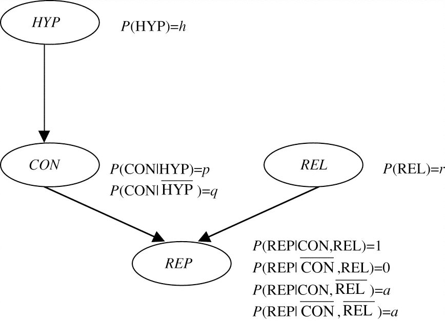
In the case at hand, whether the test consequence holds is directly influenced by and only by whether the hypothesis is true or not; whether there is a report to the effect that the test consequence holds is directly influenced by and only by whether the test consequence holds or not and by whether the instrument is reliable or not. Hence, we construct the basic graph in Figure 2.1 in which the node with the variable HYP is a parent node to the node with the variable CON and the nodes with the variables CON and REL are in turn parent nodes to the node with the variable REP. Furthermore, root nodes are unparented nodes and descendant nodes are child nodes, or child nodes of child nodes etc. E.g., HYP and REL are root nodes and CON and REP are descendant nodes of HYP in our graph.

Figure 2.1.

The basic model for testing with a LTFR instrument.

From DAG to Bayesian Network, one more step is required. We need to stipulate a probability distribution for the variables in the root nodes of the graph and a conditional probability distribution for the variables in the other nodes given any combination of values of the variables in their respective parent nodes.

Let us turn to our example. First, we take care of the root nodes, i.e. we assign a prior probability to the hypothesis and to the reliability of the instrument:

Second, consider the node with the variable CON which is a child node to the node with the variable HYP. We take a broad view of what constitutes a test consequence, that is, we do not require that the truth of the hypothesis is either a necessary or a sufficient condition for the truth of the test consequence. Rather, a test consequence is to be understood as follows: the probability of the consequence given that the hypothesis is true is greater than the probability of the consequence given that the hypothesis is false:

Third, consider the node with the variable REP, which is a child node to the nodes with the variables CON and REL. How can we model the workings of an unreliable instrument? Let us make an idealization: we suppose that we do not know whether the instrument is reliable or not, but if it is reliable, then it is fully reliable and if it is not reliable, then it is fully unreliable. Let a fully reliable instrument be an instrument that provides maximal information: it is an instrument that says of what is that it is, and of what is not that it is not:

Let a fully unreliable instrument be an instrument that provides minimal information: it is an instrument that is no better than a randomizer:

Let us call a the randomization parameter. (Compare Bovens and Olsson Reference Bovens and Olsson2000, 701–703 for this construction.) We can now construct the Bayesian Network by adding the probability values to the graph in Figure 2.1.

The arrows in a Bayesian Network have a precise probabilistic meaning: they carry information about the independence relations between the variables in the Bayesian Network. This information is expressed by the Parental Markov Condition:

1. (PMC) A variable represented by a node in the Bayesian Network is independent of all variables represented by its non-descendant nodes in the Bayesian Network, conditional on all variables represented by its parent nodes.

Hence, our Bayesian Network is constructed on grounds of the following (conditional) independences:

(7) says that if one does not know any values of the variables, then coming to learn that the instrument is reliable or that the instrument is unreliable does not alter the prior probability that the hypothesis is true. This is a plausible assumption as long as one's reasons for believing that the instrument is reliable are independent of the truth of the hypothesis. In Section 5, we will investigate what happens when this assumption is violated. (8) says that if one knows no more than that the hypothesis is true or that the hypothesis is false, then coming to learn in addition that the instrument is reliable or that it is unreliable does not alter the probability that the test consequence holds: as long as one does not know what report the instrument provides, coming to learn about its reliability teaches us nothing about the test consequence. (9) says that if one knows no more than that some definite values of REL and CON are instantiated, then coming to learn in addition that some definite value of HYP is instantiated does not alter the probability of REP: the chance that the instrument will yield a positive or a negative report is fully determined by whether the instrument is reliable and whether the test consequence holds or not; once this information is known, the truth or falsity of the hypothesis itself becomes irrelevant. The latter two assumptions seem beyond reproach.

The Bayesian Network also represents a series of other conditional independences, e.g. REP ╨ HYP|CON. These independences can be derived by means of the semi-graphoid axioms, which are a set of axioms of conditional independence, from the conditional independences that can be read off the diagram by applying the (PMC). There is also a convenient criterion, viz. the d-separation criterion, which permits us to read these same conditional independences directly off of the graph. For the details, we refer to the relevant literature.Footnote 1

What's so great about Bayesian Networks? A Bayesian Network contains information about the independence relations between the variables, prior probability assignments for each root node and conditional probability assignments for each child node given its parent nodes. A central theorem in the theory of Bayesian Networks states that a joint probability distribution over any combination of values of the variables in the network is equal to the product of the prior probabilities and conditional probabilities for these values as expressed in the network (Neapolitan Reference Neapolitan1990, 162–164). For example, suppose we are interested in the joint probability of HYP, $\overline{\mathrm{CON}\,}$, REP and $\overline{\mathrm{REL}\,}$. We can read the joint probability directly off Figure 2.1:

Standard probability calculus teaches us how to construct marginal distributions out of joint distributions and subsequently conditional distributions out of marginal distributions.

We are interested in the probability of the hypothesis given that there is a report from a LTFR instrument that the test consequence holds. This probability is P*(HYP) = P(HYP|REP) = P(HYP, REP)/P(REP). For ease of representation, we will abbreviate (1 − x) as $\overline{x}$.

We measure the degree of confirmation that the hypothesis receives from a positive report by the difference:

Note that P*(HYP) − P(HYP) > 0 iff p > q. To have some numerical data, let h = r = a = 1/2 and let p = 3/4 and q = 1/4. Then P*(HYP) = 5/8 and P*(HYP) − P(HYP) = 1/8.

We know now how to model the degree of confirmation that a hypothesis receives from a single positive report concerning a single test consequence of the hypothesis by means of a single LTFR instrument. This basic model will be the paradigm for modelling complex strategies to improve the degree of confirmation that can be obtained from LTFR instruments.

3. Same Test Results

Suppose that we have tested a single test consequence of the hypothesis by means of a single LTFR instrument. We have received a positive report, but we want to have additional confirmation for our hypothesis. We might want to run more tests of the very same test consequence. Now there are two possibilities. Either we can take our old LTFR instrument and run the test a couple more times. Or we can choose new and independent LTFR instruments and test the very same test consequence with these new instruments. First, we will show that both of these substrategies can be successful: if we receive more reports to the effect that the test consequence holds, either from our old instrument or from new and independent instruments, then the hypothesis does indeed receive additional confirmation. Second, we are curious to know which substrategy is the better strategy assuming that we do indeed receive more reports to the effect that the test consequence holds. In other words, which substrategy yields a higher degree of confirmation? Is there an univocal answer to this question, or is one substrategy more successful under certain conditions, while the other strategy is more successful under other conditions? To keep things simple, we will present our analysis for one additional test report, either from the same or from different LTFR instruments.

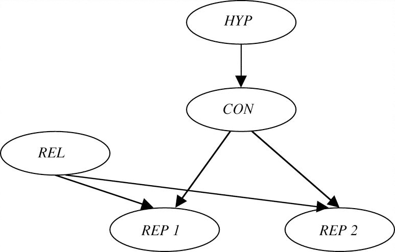
Let us first model the degree of confirmation that the hypothesis receives from an additional positive report from the same LTFR instrument. In Figure 3.1, we add a node to our basic graph to represent the binary variable REP2 and substitute REP1 for REP. Just like REP1, REP2 is directly influenced by REL and CON and so two more arrows are drawn in. We impose a condition of symmetry on the probability distribution P for this graph and also require, for this second report, that the instrument is either fully reliable or it is fully unreliable with the same randomization parameter a.

Figure 3.1.

Multiple measurements with a single instrument of a single consequence.

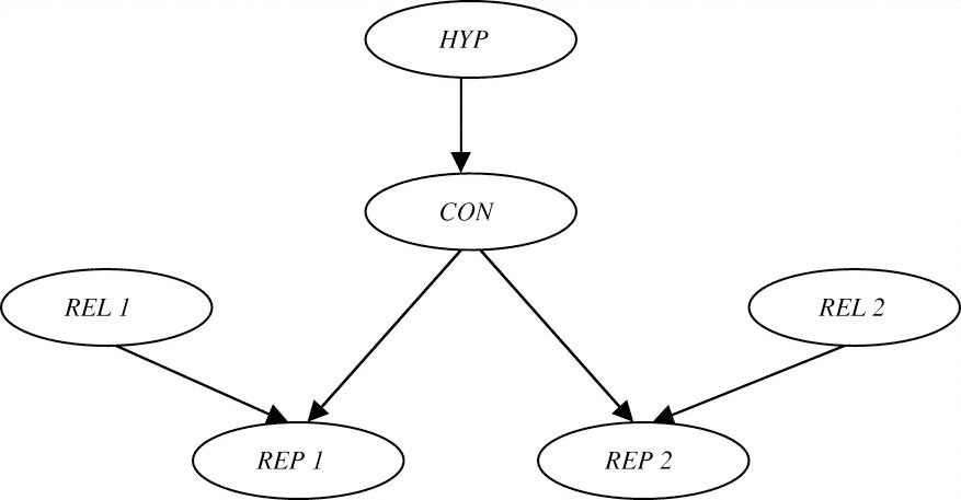
Secondly, we model the degree of confirmation that the hypothesis receives from an additional confirming report from a second independent LTFR instrument. In Figure 3.2, we add a node to our basic graph for the variable REL2 which expresses whether the second instrument is reliable or not and add a node for the variable REP2 which expresses whether the second instrument provides a report to the effect that the test consequence holds or not. REP2 is directly influenced by REL2 and CON: we draw in two more arrows. To keep matters simple, we impose a condition of symmetry on the probability distribution P′ for this graph: there is an equal chance r that both instruments are reliable and if the instruments are unreliable then they randomize at the same level a. To compare the scenario with one instrument to the scenario with two instruments we need to impose a ceteris paribus condition: for this reason we postulate the same values h, p, q, r and a for the probability distributions P and P′.

Figure 3.2.

Measurements with multiple instruments of a single consequence.

The instruments are independent of one another. What this means is that

Suppose that we know that the consequence holds or we know that the consequence does not hold. Then there is a certain chance that we will receive a report to the effect that the consequence holds. Now whether we receive another report to this effect or not, does not affect this chance. An independent instrument may not always provide us with an accurate report, but it is not influenced by what other instruments report. It can be shown that (13) is a conditional independence that can be read off from the graph in Figure 3.2.

Are these strategies successful? The strategy of searching out an additional report from the same LTFR instrument about the same test consequence always provides additional confirmation to the hypothesis:

1. Theorem 1. ΔP = P(HYP|REP1,REP2) −P(HYP|REP1) > 0.

(All theorems are proven in the appendix.) The strategy of searching out an additional report from a different LTFR instrument about the same test consequence always provides additional confirmation to the hypothesis:

1. Theorem 2. ΔP = P′(HYP|REP1,REP2) − P′(HYP|REP1) > 0.

We turn to the question whether, ceteris paribus, the hypothesis receives more confirmation from a second positive report from one and the same LTFR instrument or from independent LTFR instruments. We show in the appendix that

1. Theorem 3. ΔP = P′(HYP|REP1,REP2) −P(HYP|REP1,REP2) iff 1 − 2$\overline{a}$$\overline{r}$ > 0.

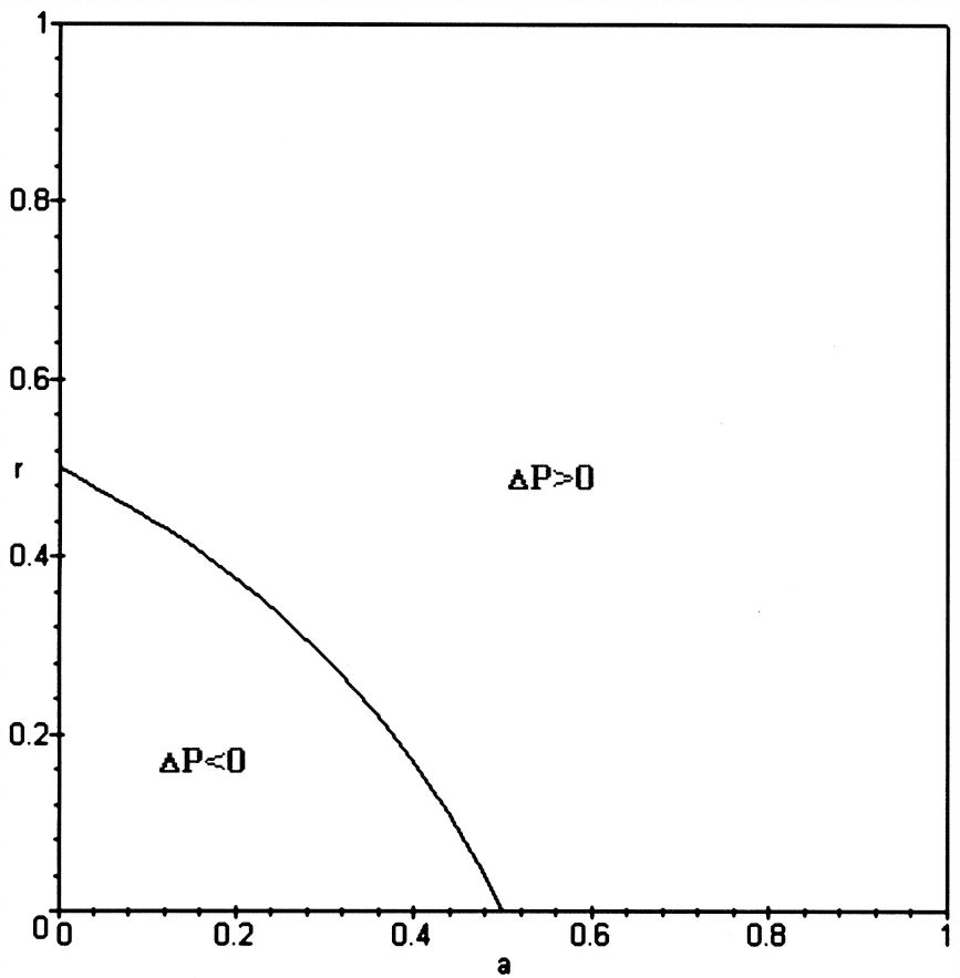
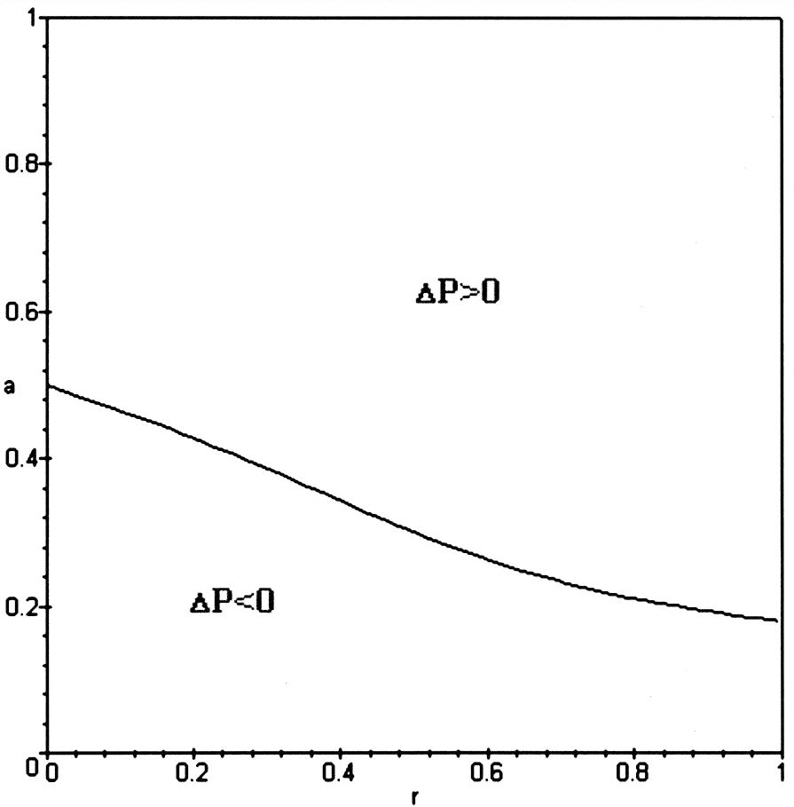
The graph in Figure 3.3 represents this inequality. For values of (a,r) above the phase curve, ΔP > 0, i.e. it is better to receive reports from two instruments; for values of (a,r) on the phase curve, ΔP = 0, i.e. it does not make any difference whether we receive reports from one or two instruments; for values of (a,r) below the phase curve, ΔP < 0, i.e. it is better to receive reports from one instrument than from two instruments.

Figure 3.3.

ΔP > 0 iff positive reports from two instruments testing the same consequence yield more confirmation to the hypothesis than from a single instrument.

Do these results seem plausible at an intuitive level? There are two conflicting intuitions at work here. On the one hand, we are tempted to say that confirming results from two instruments is the better way to go, since independence is a good thing. On the other hand, if we receive consistent positive reports from a single instrument, then we feel more confident that the instrument is not a randomizer and this increase in confidence in the reliability of the instrument supports the confirmation of the hypothesis. For higher values of r, the former consideration becomes more weighty than the latter: there is not much gain to be made anymore in our confidence in the reliability of the instrument(s) and we might as well enjoy the benefits of independence. For lower values of a, the latter consideration becomes more weighty: if we are working with an instrument which, if unreliable, has a low chance of providing positive reports, then consistent positive reports constitute a substantial gain in our confidence in its reliability, which in turn supports the confirmation of the hypothesis.

4. Coherent Test Results

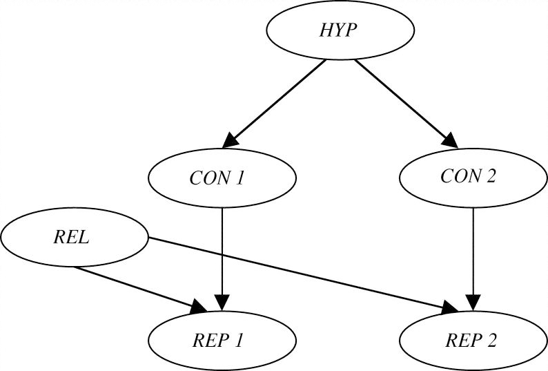
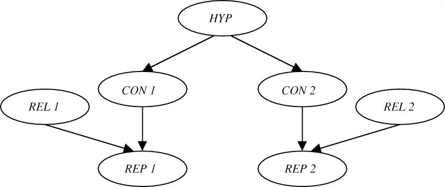
The second strategy to raise the degree of confirmation for a hypothesis is to identify a range of test consequences which can all be assessed by a single or by multiple independent LTFR instruments. Let us draw the graphs for two test consequences. Following our heuristic, the hypothesis (HYP) directly influences the test consequences (CONi for i = 1,2). Figure 4.1 represents the scenario in which there is a single instrument: each test consequence (CONi) conjoint with the reliability of the single instrument (REL) directly influences the report about the consequence in question (REPi). Figure 4.2 represents the scenario in which there are two independent instruments: each test consequence (CONi) conjoint with the reliability of the instrument that tests this consequence (RELi) directly influences the report about the consequence in question (REPi). We define a probability distribution P for the DAG in Figure 4.1 and a probability distribution P′ for the DAG in Figure 4.2. We impose the symmetry condition within each distribution and the ceteris paribus condition between distributions for all the relevant parameters.

Figure 4.1.

Measurements with a single instrument of multiple consequences.

Figure 4.2.

Measurements with multiple instruments of multiple consequences.

We can now check whether our strategies are successful. It turns out that the strategy is always successful with multiple instruments:

1. Theorem 4. ΔP = P′(HYP|REP1, REP2) − P′(HYP|REP1) > 0.

But with a single instrument, the strategy is not always successful:

1. Theorem 5. ΔP = P(HYP|REP1, REP2) − P(HYP|REP1) > 0 iff pqr + $a\overline{r}$(p + q − a) > 0.

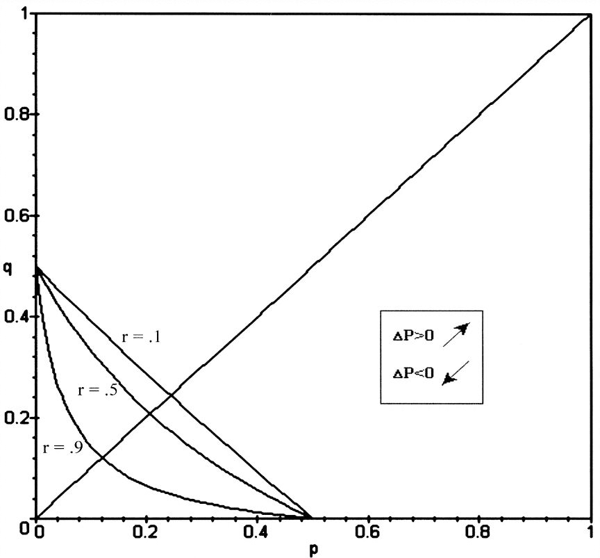
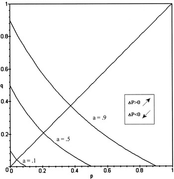
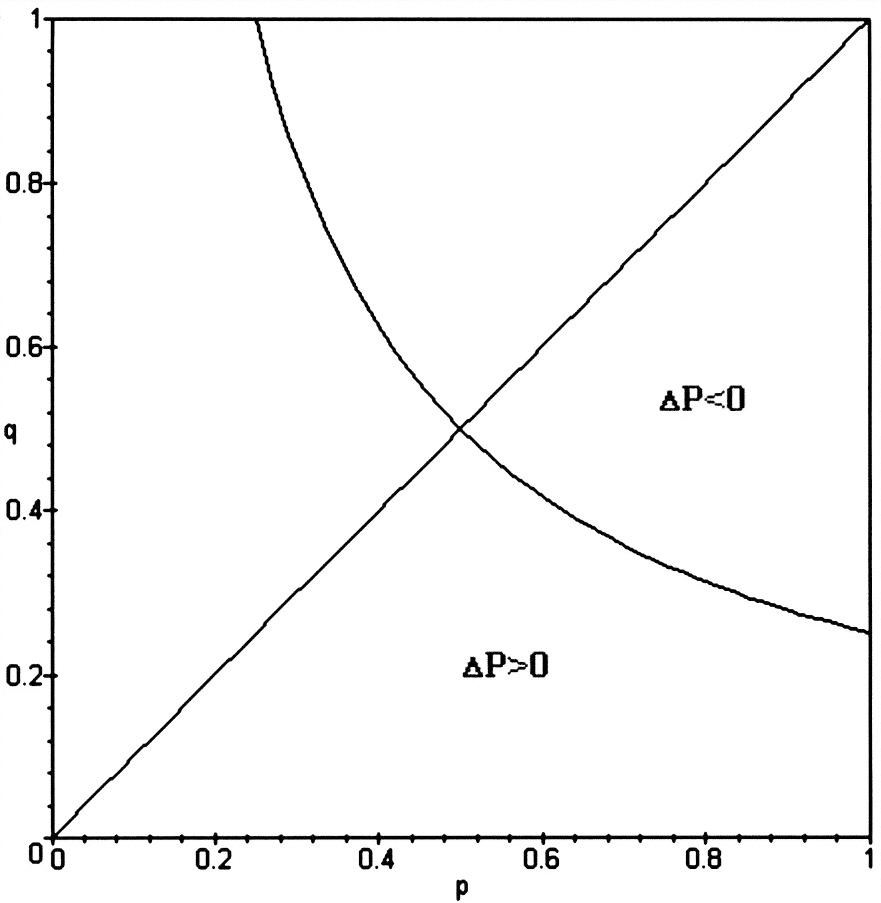
In Figure 4.3, we fix a = .5 and construct phase curves for high, medium and low range values of the reliability parameter r. In Figure 4.4, we fix r = .5 and construct phase curves for high, medium and low range values of the randomization parameter a. Since we have stipulated that p > q, we are only interested in the areas below the straight line for p = q in both figures.

Figure 4.3.

ΔP > 0 iff two positive reports from a single instrument testing two consequences yield more confirmation to the hypothesis than one positive report testing a single consequence for a = .5. The relevant region is the region where p > q.

Figure 4.4.

ΔP > 0 iff two positive reports from a single instrument testing two consequences yield more confirmation to the hypothesis than one positive report testing a single consequence for r = .5. The relevant region is the region where p > q.

The areas in these graphs in which ΔP < 0 are certainly curious: for certain values of p, q, a and r, we test a first consequence of a hypothesis, receive a positive report and are more confident that the hypothesis is true; then we test a second consequence of the hypothesis with the very same instrument, receive once again a positive report … but this time around our degree of confidence in the hypothesis drops! How can we interpret these results? Notice that the effect is most widespread for (i) lower values of r, (ii) higher values of a and (iii) lower values of p. To get a feeling for the magic of the numbers, let us look at this range of values, where the effect occurs par excellence. Hence, let us consider instruments which are not likely to be reliable, and, if unreliable, have a high chance of providing a positive report, and test consequences which are unlikely to occur when the hypothesis is true (though of course the test consequences are still more likely to occur than when the hypothesis is false). Considering (i), we do not have much trust in the instrument to begin with. Now it gives us nothing but positive reports: considering (ii), the instrument is likely to be a randomizer and so we become even more confident that the instrument is unreliable. But should this not be offset by the fact that we receive coherent test results in support of our hypothesis? No, since considering (iii), our tests are rather weak and these coherence effects count for little. Hence, when we get a second positive report, we become very confident that the instrument is unreliable and consequently our confidence in the hypothesis drops.

We turn to the question whether, ceteris paribus, the hypothesis receives more confirmation from a second positive report from one and the same LTFR instrument or from independent LTFR instruments. We have shown that

1. Theorem 6. ΔP = P′(HYP|REP1,REP2) − P(HYP|REP1,REP2) > 0 iff (2a − p − q)a − 2(a − p)(a − q) r > 0.Footnote 2

To evaluate this expression, we assume that the tests are reasonably strong by fixing p = .9 and q = .1 and construct a phase curve for values of (a,r) in Figure 4.5. If the randomization parameter and the reliability parameter are set low, then one instrument tends to do better than two. Subsequently we assume mid-range values for the randomization and the reliability parameters (a = .5 and r = .5) and construct a phase curve for values of (p,q) in Figure 4.6. We are interested in the area below the straight line where p > q. If the q-value is set high, i.e. if the test consequences occur frequently also when the hypothesis is false, then one instrument tends to do better than two.

Figure 4.5.

ΔP > 0 iff positive reports from two instruments testing two consequences yield more confirmation to the hypothesis than positive reports from a single instrument testing two consequences for p = .9 and q = .1.

Figure 4.6.

ΔP > 0 iff positive reports from two instruments testing two consequences yield more confirmation to the hypothesis than positive reports from a single instrument testing two consequences for a = .5 and r = .5. The relevant region is the region where p > q.

In the previous section, we explained why the consideration that our confidence in the reliability of a single instrument is boosted by coherent positive reports outweighs the consideration of the independence of multiple instruments for lower values of a and r. The same explanation can be repeated here. But why is this effect amplified for higher q-values? The higher the q-values, the more likely the test consequences will hold true and so coherent positive reports will boost our confidence in the reliability of a single instrument even more. Hence higher q-values tend to favor a single over multiple instruments.

It is one of the textbook Bayesian success stories that an account can be provided of why variety of evidence is a good thing: it is shown that the increment of confirmation that the hypothesis receives from confirming test results becomes smaller and smaller as we run the same old test over and again. (E.g. Earman Reference Earman1992, 77–79 and Howson and Urbach Reference Howson and Urbach1993, 119–123.) But what does it mean to run the same old test over and over again? We could take it to mean that we check the same old test consequences rather than checking independent test consequences of the hypothesis. Or we could take it to mean that we do our testing with the same old instrument rather than with independent instruments. Presumably variety of evidence refers to multiple consequences as well as to multiple instruments.

We have in effect tested the variety-of-evidence thesis under this particular interpretation. There are two sets of evidence, one containing a less varied pair and one containing a more varied pair of positive test reports. To respect the ceteris paribus clause, we assume that each item of evidence i = 1,2 within these sets j = 1,2 has the same evidential strength, as expressed by the likelihood ratio P(REPi^j|HYP)/P(REPi^j|$\overline{\mathrm{HYP}\,}$). This ceteris paribus clause can be justified by means of the following analogy. Suppose one wants to test the claim that a varied set of investments promises a greater yield than a non-varied set. Then it would clearly be wrong to compare a varied set of investments that each have a high rating and a non-varied set of investments that each have a low rating, or vice versa: the ceteris paribus clause require that each investment within the respective sets has the same rating. Similarly, the ceteris paribus clause in this context requires that each item of evidence within the respective sets has the same evidential strength.Footnote 3 Given this the variety-of-evidence thesis implies that a hypothesis receives more confirmation from a more varied set of evidence than a less varied set of evidence, ceteris paribus, in which more varied evidence is taken to mean evidence that is obtained from multiple instruments rather than a single instrument or evidence that reports on multiple consequences rather than a single consequence.

However, our investigation permits us to impose the following caveats concerning this interpretation of the thesis. We argued in Section 3 that,

1. (i) if we are testing a single consequence, it is sometimes more beneficial for the confirmation of the hypothesis to receive positive reports from the same instrument than from different instruments, ceteris paribus.

What we have seen in this section is that,

1. (ii) if we are testing different consequences, it is sometimes more beneficial for the confirmation of the hypothesis to receive positive reports from the same instrument than from different instruments, ceteris paribus.

And there is still another conclusion to be drawn from our results. We saw in the previous section that it is always a good thing for the confirmation of the hypothesis to receive a second positive report from the same instrument about the same test consequence. In this section, we saw that our confidence in the hypothesis may decrease as we receive a second positive report from the same instrument about a different test consequence. Hence, we can add a third caveat:

1. (iii) If we are testing with a single instrument, it is sometimes more beneficial for the confirmation of the hypothesis to receive positive reports about the same consequence rather than about different consequences, ceteris paribus.

There are two Bayesian approaches to the problem of the variety of evidence present in the literature (Wayne Reference Wayne1995). On the correlation approach, the items of evidence E₁, …, E_n are less varied the greater the rate of increase in the probability values P(E₁), P(E₂|E₁), …, P(E_n|E₁, …,E_n−1) (Howson and Urbach Reference Howson and Urbach1993, 119–123; Earman Reference Earman1992, 77–79). On the eliminative approach, a set of evidence E in support of the hypothesis H_i is more varied, the lower the likelihoods P(E|H_j) for j = 1, …, i−1, i+1, …, n: varied evidence is evidence that permits us to exclude more competing hypotheses (Horwich Reference Horwich1982, 118–122 and Wayne Reference Wayne1995, 116). Each of these approaches starts from a particular pretheoretical intuition about diversity. Our approach does no less: the pretheoretical intuition that we start with is that evidence that proceeds from multiple instruments and that addresses multiple test consequences is more varied than evidence that proceeds from a single instrument or that addresses a single test consequence.

How does our analysis compare to the correlation approach? It can easily be shown that P(REP1) = P′(REP1) in all of our comparative cases. Hence, a set of evidence is the less varied on the correlation approach, the more P(REP2|REP1) exceeds P(REP2) for P = P, P′, which is indeed the case for single (as opposed to multiple) instruments and for single (as opposed to multiple) test consequences. However, what our analysis shows is that this is no guarantee that the confirmation that the hypothesis receives will be smaller. For instance, consider the cases that are modeled by the Figures 3.1 and 3.2. Set h = .5, p = .9, q = .1, a = .2 and r = .2 in both distributions. Then the prior probability P(REP1) = P′(REP2) = .26 is the same, but there is a stricter correlation and hence less variety of evidence when the reports come from a single instrument than from two independent instruments, viz. P(REP2|REP1) ≈ .51 > .30 ≈ P′(REP2|REP1). However, the hypothesis receives more confirmation when the reports come from a single rather than from one instrument, viz. P(HYP|REP1,REP2) ≈ .80 > .77 ≈ P′(HYP|REP1,REP2). Then how is it that formal results were established in the correlation approach? This approach makes the assumption that the evidence is strictly entailed by the hypothesis, viz. P(E|H) = 1. This is a restrictive constraint on the notion of evidence and quite unrealistic in many contexts, e.g. in the context of the diagnosis of disease. What our examples show is that less varied evidence may indeed provide more confirmation to the hypothesis, if we work with a looser notion of evidence and relax the assumption to P(E|H) = p > q = P(E|$\overline{\mathrm{H}\,}$).

Let us turn to the eliminative approach. Fitelson (Reference Fitelson1996, 654–656) argues that the eliminative approach requires the additional ceteris paribus assumption that the likelihoods of both sets of evidence on the hypothesis i must be identical. What is the import of the eliminative approach when there are only two hypotheses, viz. H and $\overline{\mathrm{H}\,}$, as is the case in our examples? Suppose that we want to ascertain whether a patient in a hospital has Lyme disease (H). One set of evidence E contains vomiting, fever, … Another set of evidence E′ contains a recent tick bite, a characteristic rash, … It is plausible to set P(E|H) = P(E′|H) and P(E|$\overline{\mathrm{H}\,}$) > P(E′|$\overline{\mathrm{H}\,}$). Then on the eliminative approach, E′ is more varied than E. Fitelson's ceteris paribus condition is not satisfied, since P(REP1,REP2|HYP) ≠ P′(REP1,REP2|HYP) in any of the cases that we are comparing. We do not find this disconcerting, since the eliminative notion of variety of evidence is really a stretch of the ordinary notion. Certainly E′ has more diagnostic value than E, but is this due to it being more diverse? Note that, on the eliminative approach, a single item of evidence could be more varied than some other single item of evidence, which seems somewhat odd. What the eliminative approach seems to capture is how ‘diversifying’ the evidence is, i.e. what its capability is to distinguish between competing hypotheses. Furthermore, even if a case can be made that this notion corresponds to an intuitively plausible notion of variety of evidence, the notion we are trying to capture is still very different from the notion that is sought after in the eliminative approach.Footnote 4

5. Auxiliary Theories

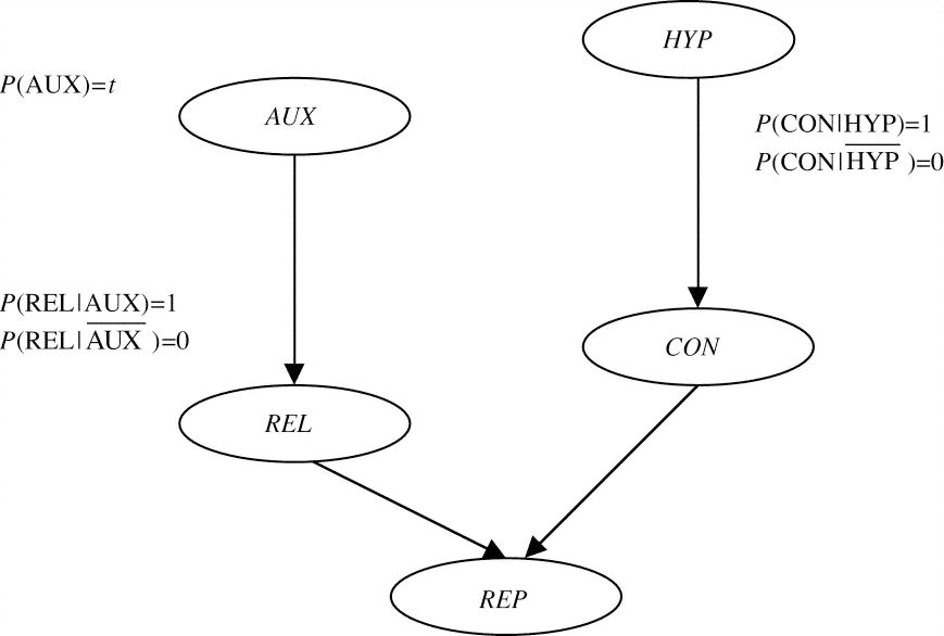
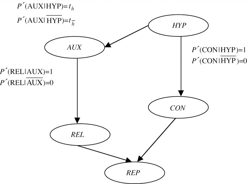
Let us return to our basic model from Section 2. In this model, the variable REL is a root node and we have assigned a probability value r which expresses the chance that the instrument is reliable. It is a common theme in contemporary philosophy of science that the workings of the instrument are themselves supported by an auxiliary theory of the instrument. If this is the case, then we should not model REL as a root node: whether the instrument is reliable or not is directly influenced by whether the auxiliary theory (AUX) holds or not. Just as we assigned a prior probability to the hypothesis, we also assign a prior probability t to the auxiliary theory. To keep matters simple, let us assume in this section that the instrument is reliable just in case the auxiliary theory is correct and that the test consequence holds just in case the hypothesis is true. Our basic model is then expanded to the Bayesian Network in Figure 5.1. In this Bayesian Network, AUX and HYP are still independent. This may or may not be a realistic assumption. Sometimes the auxiliary theory has no relation whatsoever to the hypothesis under test. But sometimes they are quite closely tied to each other: for instance, they may both be parts of a broader theory. We can model this positive relevance between AUX and HYP by connecting both variables in the Bayesian Network and by setting P′(AUX|HYP) = t _h > $t_{\overline{h}}$ = P′(AUX|$\overline{\mathrm{HYP}\,}$) as in Figure 5.2.

Figure 5.1.

The reliability of the instrument is supported by an independent auxiliary theory.

Figure 5.2.

The reliability of the instrument is supported by a positively relevant auxiliary theory.

Here are some questions:

1. (i) Ceteris paribus, does the hypothesis receive more or less confirmation if the auxiliary theory that supports the reliability of the instrument is independent rather than positively relevant to the hypothesis under test?

2. (ii) Suppose that we receive a report from a LTFR instrument which provides confirmation for the hypothesis. We now appeal to an auxiliary theory which provides support for the reliability of the instruments, i.e. by bringing in an auxiliary theory we succeed in raising the reliability parameter r. Our question is the following: is this, ceteris paribus, a successful strategy for increasing the degree of confirmation of the hypothesis,

   1. (a) if the auxiliary theory is independent of the hypothesis;

   2. (b) if the auxiliary thesis is positively relevant to the hypothesis?

Let us first take up question (i). To respect the ceteris paribus clause we must make sure that the randomization parameter, the reliability parameter and the prior probability of the hypothesis are fixed across both scenarios. To fix the reliability parameter, we must make sure t = t _h h + t _h $\overline{h}$, since the instrument is reliable just in case the auxiliary theory is true. We have shown that:

1. Theorem 7. ΔP = P(HYP|REP) − P′(HYP|REP) > 0 iff h + $\overline{a}$(ht _h + $ht_{\overline{h}}$ − 1) > 0.

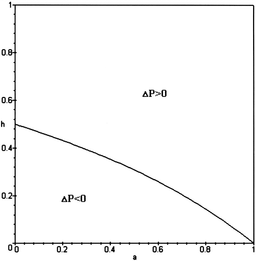
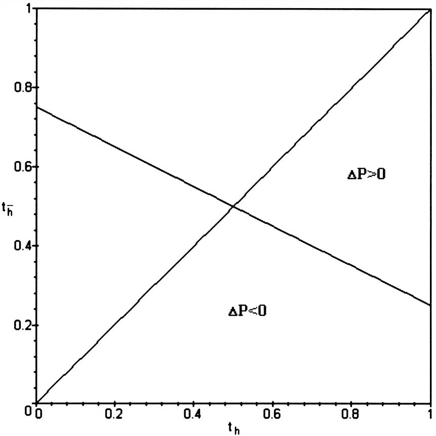
To evaluate this expression, we construct two graphs: in Figure 5.3, we set t _h = .8 and $t_{\overline{h}}$ = .2 and construct a phase curve for (a,h); in Figure 5.4, we set a = 1/3 and h = 1/3 and construct a phase curve for (t _h, $t_{\overline{h}}$).

Figure 5.3.

ΔP > 0 iff the hypothesis receives additional confirmation when the reliability of the instrument is supported by an independent rather than a positively relevant auxiliary theory with t _h = .8 and $t_{\overline{h}}$ = .2.

Figure 5.4.

ΔP > 0 iff the hypothesis receives more confirmation when the reliability of the instrument is supported by an independent rather than a positively relevant auxiliary theory with a = 1/3 and h = 1/3. The relevant region is the region where t _h > $t_{\overline{h}}$.

What we see in Figure 5.3 is that a positively relevant auxiliary theory provides more of a boost to the degree of confirmation that the hypothesis receives from a positive test report than an independent auxiliary theory for lower prior probability values of the hypothesis and for lower values of the randomization parameter. In Figure 5.4 we are only interested in the area below the line where t _h > $t_{\overline{h}}$. What we see is that for t _h < 1/2, a positively relevant auxiliary theory always provides more of a boost to the degree of confirmation of the hypothesis, while for t _h > 1/2, a positively relevant auxiliary theory provides more of a boost for and only for values of $t_{\overline{h}}$ that are sufficiently smaller than t _h, in other words, for a theory that is sufficiently positively relevant to the hypothesis.

Can an intuitive account be given of these results? Why does a positively relevant auxiliary yield a higher degree of confirmation for an implausible hypothesis than an independent auxiliary, as we can read off of Figure 5.3? If h is low, say h = .1, then a positively relevant auxiliary has a low prior probability t = (.8)(.1) + (.2)(.9) = .26. The ceteris paribus clause requires that we set the prior probability of an independent auxiliary at .26 as well. Since the hypothesis is improbable, it is likely that a positive report is due to the unreliability of the instrument and hence the falsity of the auxiliary: e.g. for a = .5, the posterior probability of the auxiliary slides below .26. However, the blame falls much more heavily on the independent auxiliary than on the positively relevant auxiliary, because the probability of the latter is tied to the probability of the hypothesis: actually, the posterior probability of the independent auxiliary goes into free fall to ≈.07 while the posterior probability of the positively relevant auxiliary remains at a respectable .17. With this distrust in the auxiliary and hence in the instrument it is understandable that the hypothesis will receive less confirmation from a positive report when the instrument is supported by an independent auxiliary than when it is supported by a positively relevant auxiliary: actually, the posterior probability of the hypothesis is .20 with a positively relevant auxiliary as opposed to ≈.16 with an independent auxiliary. Furthermore, this argument will take effect when the auxiliary is sufficiently positively relevant to the hypothesis, which we can read off Figure 5.4.

Let us now turn to our next question (ii.a). We have received a report from a LTFR instrument to the effect that some test consequence is true. Subsequently, we increase our confidence in the reliability of the instrument by appealing to an auxiliary theory that is independent of the hypothesis under test. Is this a successful strategy for increasing the degree of confirmation of our hypothesis?

It is easy to see that the answer to this question is univocally positive. Our basic model in Figure 2.1 captures the situation before some auxiliary theory in support of our hypothesis has been spotted. The model in Figure 5.1 captures the situation after some auxiliary theory has been spotted. We specify a probability distribution P for the Bayesian Network in Figure 2.1 and P′ for the Bayesian Network in Figure 5.1. To respect the ceteris paribus clause, we specify the same values a, h, p, and q for both distributions, but we choose r for P and t for P′ so that P(REL) < P′(REL). Then the following theorem holds:

1. Theorem 8. ΔP = P′(HYP|REP) − P(HYP|REP) > 0.

Matters are not as simple when we turn our attention to the last question (ii.b). What happens if we increase our confidence in the reliability of the instrument by appealing to an auxiliary theory and the auxiliary theory and the hypothesis are positively relevant to one another? To investigate this question, we raise the reliability of the instrument by bringing in a positively relevant auxiliary theory: we construct a probability distribution P for our basic model in Figure 2.1 and a probability distribution P′ for the Bayesian Network in Figure 5.2, carefully picking r, t _h and $t_{\overline{h}}$, so that r = P(REL) < P′(REL) = r* and, to respect the ceteris paribus clause, so that (ii) P(HYP) = P′(HYP). We have shown that:

1. Theorem 9. ΔP = P′(HYP|REP) − P(HYP|REP) > 0 iff ($\overline{a}$$\overline{r}$ − h)t _h + (a + $\overline{a}$r) r* − $\overline{h}$r > 0.

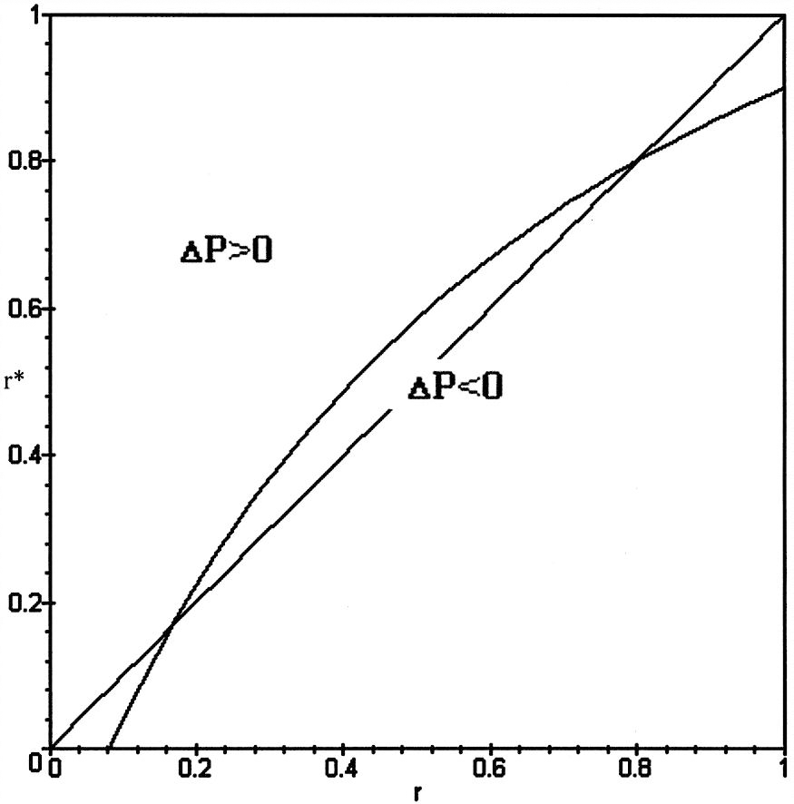
In Figure 5.5, we set the values at h = .5, a = .4 and t _h = .8 and construct a phase curve for values of (r, r*). The part of the graph that interests us is the area above the line where r* > r. In the area above the phase curve a positively relevant auxiliary theory increases the degree of confirmation for the hypothesis. In the area underneath the phase curve a positively relevant auxiliary theory decreases the degree of confirmation for the hypothesis. Notice that there exists a region underneath the phase curve where r* > r. This is curious. Here is how the story goes for this region. We are about to test a hypothesis, but are not confident about the reliability of our instrument: we realize that our confidence in the hypothesis would not increase drastically even if we were to receive a positive report. We try to boost our confidence in the reliability of the instrument and consult an expert. The expert provides us with an auxiliary theory. The auxiliary theory is uncertain, but still boosts our confidence in the reliability of the instrument. It is positively relevant to the hypothesis, but the relevant probability values are such that the prior probability of the hypothesis remains unaffected. It turns out that we will now be less confident that the hypothesis is true after a positive test report comes in than had we not consulted the expert!

Figure 5.5.

ΔP > 0 iff the hypothesis receives more confirmation when we increase the reliability of the instrument by means of a positively relevant auxiliary theory. The relevant region is ther region where r* > r.

The phenomenon is definitely curious, but a moment's reflection will show that it was to be expected given our discussion of question (i) and question (ii.a). Suppose that we have no theoretical support for the reliability of our instrument and that the reliability parameter is set at r. Clearly, the hypothesis receives precisely the same degree of confirmation when the reliability parameter has the same value r but rests on the support of some independent auxiliary theory. From our discussion of question (i), we also know that support from an independent as opposed to a dependent auxiliary theory can be better or worse for the degree of confirmation of a hypothesis, depending on the values of h, a, t _h and $t_{\overline{h}}$. So let us assume that an independent auxiliary theory raises the reliability parameter from r to r + ∊, for some small ∊. From our discussion of question (ii.a) we know that this increase will slightly raise the degree of confirmation for the hypothesis. But it is to be expected that this small raise would have been offset, if support had been sought from a dependent auxiliary theory yielding a reliability value of r + ∊, at least for particular values of the relevant parameters. Hence, finding support in a dependent auxiliary theory for the reliability of the instrument may lower the degree of confirmation for the hypothesis.

The Duhem-Quine thesis notoriously states that if our experimental results are not in accordance with the hypothesis under investigation, there is no compelling reason to reject the hypothesis, since the blame could just as well fall on the auxiliary theories. One virtue of our model is that it gives a precise Bayesian account of how experimental results affect our confidence in the hypothesis and our confidence in the auxiliary theory. But there is also a more important lesson to be learned. In discussing the Duhem-Quine thesis, Bayesians typically assume that the auxiliary theory and the hypothesis are independent (cf. Howson and Urbach Reference Howson and Urbach1993, 139), although there is some cursory discussion of dependence between the hypothesis and the auxiliary theory in Dorling (Reference Dorling1996). The assumption of independence certainly makes the calculations more manageable, but it does not square with the holism that is the inspiration for the Duhem-Quine thesis. Not only are experimental results determined by a hypothesis and auxiliary theories, they are determined by a hypothesis and auxiliary theories that are often hopelessly interconnected with each other. And these interconnections raise havoc in assessing the value of experimental results in testing hypotheses. There is always the fear that the hypothesis and the auxiliary theory really come out of the same deceitful family and that the lies of one reinforce the lies of the others. What our results show is that this fear is not entirely ungrounded: for hypotheses with a high prior probability, it is definitely better that the reliability of the instrument be supported by an independent auxiliary theory. But on the other hand, for hypotheses with a low prior probability, we should cast off such fears: hypotheses and auxiliary theories from the same family are very welcome, since positive test reports provide stronger confirmation of the hypothesis under consideration.

6. Calibration

To raise the degree of confirmation of the hypothesis that a particular test result from a LTFR instrument has provided, we can try to increase our confidence in the LTFR instrument by calibrating it. Consider an example: we have a test result in our hands from a LTFR technique for dating artifacts in archeology. A simple form of calibration is to set the technique to work on some artifacts that have their dates chiseled into them (by a reliable stone mason) and to check whether the technique indeed provides the correct output. If so, then we can feel more confident that the technique is indeed reliable and subsequently that the test result and the hypothesis are correct. Let us model this simple form of calibration in a Bayesian Network before moving on to the more complex form in which the LTFR instrument is calibrated against test results from other LTFR instruments.

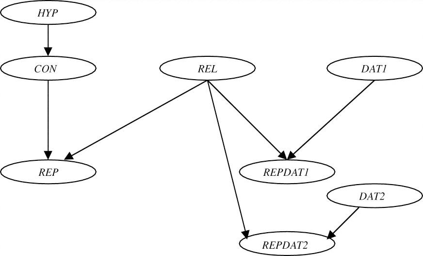
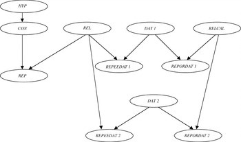
Suppose that we have a single report from a LTFR instrument and that the content of this report is a test consequence of some hypothesis. This set up is captured by our basic model in Section 2. Subsequently, we identify a series of data that are roughly of the same nature as the test consequence in question but which we are confident are true. The LTFR instrument is then calibrated by examining whether it yields correct values for these data. To keep things simple, we will model a case with two data (DAT1 and DAT2). Following our heuristic, the reports about these data (REPDAT1 and REPDAT2) are directly influenced by the reliability of the instrument in question and by whether the data are true or not. This yields the graph in Figure 6.1.

Figure 6.1.

Calibrating the instrument against certain data.

We assign a probability value of 1 to DAT1 and DAT2 in line with our stipulation that we have chosen certain data. Nothing would prevent us of course from inserting lower degrees of confidence into our model. The graph displays a series of independences. One such independence is worth focusing on, since it does reflect a substantial simplification:

The data are independent of the test consequence and are independent of one another. This is a plausible assumption for artifacts that are sufficiently heterogeneous: say, if they are not found on the same site, are not similar in style etc.

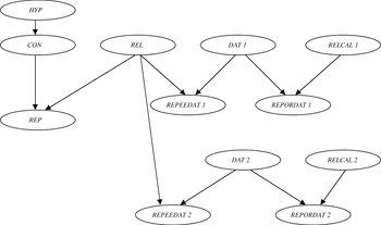
We can now turn to a more complex form of calibration which preserves the independences of Figure 6.1. Quite often there are no clean data available against which to calibrate our instruments. Rather, we can do no better than calibrate our instrument against reports from a single or from multiple LTFR instruments about uncertain data. Let the LTFR instrument that is to be calibrated be the calibratee and the single or multiple LTFR instruments against whose reports the calibration takes place be the calibrator(s). If the calibratee yields the same reports as the calibrator(s) about these uncertain data, then we may be more confident that the calibratee is reliable and consequently that the test consequence and the hypothesis is correct. We will model this more complex form of calibration for two uncertain data DAT1 and DAT2. We receive test reports about these uncertain data from the calibratee (REPEEDAT1 and REPEEDAT2) and from the calibrator(s) (REPORDAT1 and REPORDAT2). Now we draw the following distinction: either we calibrate against the reports from a single calibrator, or we calibrate against the reports from multiple calibrators, one for each datum. In accordance with this distinction, we can draw two graphs. The variable RELCAL expresses the reliability of the single calibrator in the graph in Figure 6.2, while the variables RELCAL1 and RELCAL2 express the reliability of the respective calibrators in the graph in Figure 6.3.

We can read off a series of independences from these graphs. As before, we have made the simplifying assumption that all the instruments are independent:

We define a probability distribution over each graph and impose our usual symmetry conditions (within each distribution) and ceteris paribus conditions (between distributions). We assume that the calibrators are either fully reliable or fully unreliable; if they are fully unreliable, then they all are no better than randomizers with a common parameter a, which equals the parameter of the instrument to be tested. Let us also assume that we have the same degree of confidence in all the calibrators and the same degree of confidence in the data. P is the probability distribution for the graph in Figure 6.2 and P′ is the probability distribution for the graph in Figure 6.3. Then, for i = 1,2

It is reasonable to assume that if we are out to calibrate a LTFR instrument, then we will pick calibrators that we take to be more reliable than the calibratee, i.e. P(REL) = P′(REL) = r < s.

Figure 6.2.

Calibrating the instrument against uncertain data with a single calibrating instrument.

Figure 6.3.

Calibrating the instrument against uncertain data with multiple calibrating instruments.

What needs to be investigated is under what conditions the strategy of calibrating against data from a single more reliable instrument as well as the strategy of calibrating against data from multiple more reliable instruments are successful strategies. We consider the point in time at which the hypothesis has received confirmation from a report about the test consequence from the calibratee. Subsequently, we receive the additional information that the calibrator(s) provided the same reports about both data as the calibratee. Theorem 10 shows under what conditions the additional information from a single calibrator raises the degree of confirmation for the hypothesis:

1. Theorem 10. ΔP = P(HYP|REP,REPEEDAT1,REPEEDAT2,REPORDAT1,REPORDAT2) − P(HYP|REP) > 0 iff a ²(f ² − a ²)$\overline{s}$ + (1 − a ²)f ²s > 0.

and Theorem 11 shows under what conditions the additional information from multiple calibrators raises the degree of confirmation for the hypothesis:

1. Theorem 11. ΔP = P′(HYP|REP,REPEEDAT1,REPEEDAT2,REPORDAT1,REPORDAT2) − P′(HYP|REP) > 0 iff a(f − a)$\overline{s}$ + $\overline{a}$fs > 0.

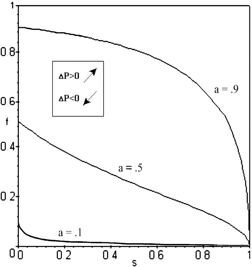
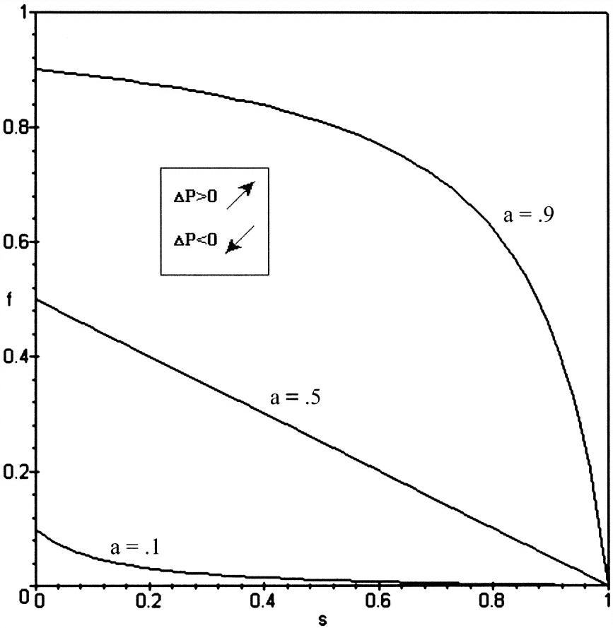
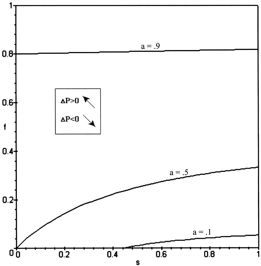
We plot phase curves for different values of the randomization parameter in the single-calibrator case in Figure 6.4. What is going on here? Focus on the area where the data are improbable (i.e. where f is low) and the reliability parameter for the calibrator is low (i.e. where s is low): in this area ΔP < 0, i.e. calibration decreases the degree of confirmation that the hypothesis receives. This is to be expected: when we get calibration results from a calibrator that is likely to be unreliable and that in addition provides positive reports about implausible data, then we become even more suspicuous of the calibratee, since it yields the same odd results as the calibrator that is likely to be unreliable. And the more suspicuous we are of the calibratee, the less confirmation the hypothesis receives. Furthermore the higher we set the randomization parameter a, the stronger this effect will become, since positive reports are the more likely to come for unreliable instruments. Figure 6.5 presents the phase curves for the case of multiple calibrators. The interpretation is similar to the case for a single calibrator.

Figure 6.4.

ΔP > 0 iff the hypothesis receives additional confirmation from matching reports from a single calibrating instrument.

Figure 6.5.

ΔP > 0 iff the hypothesis receives additional confirmation from matching reports from two calibrating instruments.

Subsequently, we are curious to know whether, ceteris paribus, the hypothesis receives more or less confirmation if we calibrate against data from a single rather than from multiple calibrators. Is there a general answer, or are there specific conditions under which it is better to calibrate against a single instrument and under which it is better to calibrate against multiple instruments? We have shown that,

1. Theorem 12. ΔP = P(HYP|REP,REPEEDAT1,REPEEDAT2,REPORDAT1,REPORDAT2) − P′(HYP|REP,REPEEDAT1,REPEEDAT2,REPORDAT1,REPORDAT2) > 0 iff (2$\overline{a}$s + a)(f − a) + a $\overline{a}$ > 0.

We plot phase curves for different values of the randomization parameter in Figure 6.6. For all the values of s and f above these curves, ΔP > 0 and for all values of s and f underneath these curves, ΔP < 0. We see that for lower f, higher s and higher a, it is better to calibrate against two rather than one calibrator. In other words, as the data become less likely, as the calibrator(s) are more likely to be reliable and as the randomization parameter grows, it is better to calibrate against two rather than one calibrator.

Figure 6.6.

ΔP > 0 iff the hypothesis receives more confirmation from matching reports from a single calibrating instrument than from two calibrating instruments.

How are we to interpret these results? There are two conflicting considerations at work in determining whether it is better to calibrate against a single as opposed to against multiple calibrators. On the one hand, we like to raise the probability that the calibrator is reliable by getting coherent reports from a single instrument. This effect will assert itself when we can assess highly plausible data, when the prior probability that the calibrator is reliable is still low, so that there is much to be gained from the coherence of the reports, and when the randomization parameter is low, so that positive reports are unlikely to come from unreliable instruments. On the other hand, there is something to be gained from having independent calibrators to improve the reliability of the calibratee. This latter consideration gains the upper hand as the conditions which were favorable to the former consideration wear off: coherent positive reports about implausible facts do not do much to boost the reliability of a single calibrator; if the single calibrator is already very likely to be reliable, then there is little to be gained anymore from coherent positive reports; and if the randomization parameter is set high, then coherent positive reports do not do much to convince us that the single calibrator is reliable, since they are likely to come from unreliable instruments. At this point more is to be gained from receiving independent reports from multiple calibrators.

Compare Figures 3.3, 4.5 and 4.6 on the one hand with Figure 6.6 on the other hand. In the former figures we compared whether it was better for the confirmation of the hypothesis to receive positive reports from one or from two instruments. Two instruments do better than a single instrument for run-of-the-mill values, such as a = r = .5, p = .8 and q = .2. In the latter figure we compared whether it was better for the confirmation of the hypothesis to obtain agreement between the test instrument and a single or multiple calibrators. One calibrator does better than two calibrators for run-of-the-mill values such as a = f = .5 and s = .8 (which exceeds r), one calibrator does better than two calibrators. In modeling strategies to receive confirmation from unreliable instruments with Bayesian Networks, it was this curious difference that first sparked our interest.

7. Concluding Remarks and Future Directions

Let us list some of the more striking results of our investigation:

1. (i) The standard strategies to deal with unreliable instruments are not always successful:for specific values of the relevant parameters, the degree of confirmation will drop rather than rise when we obtain (a) a positive report about an additional test consequence from the same LTFR instrument, (b) support for our LTFR instrument from a dependent auxiliary theory, or (c) matching reports from the LTFR instrument and the calibrating instrument(s).

2. (ii) The variety-of-evidence thesis is not sacrosanct on a plausible reading of this thesis: positive reports from single rather than from multiple LTFR instruments and positive reports about a single rather than about multiple consequences will for certain values of the relevant parameters provide more confirmation to a hypothesis, ceteris paribus. These results play havoc with the correlation approach to the variety-of-evidence thesis.

3. (iii) The Duhem-Quine thesis is no reason to despair about confirmation. An appeal to an auxiliary theory in support of a LTFR instrument can improve the degree of confirmation for the hypothesis and the interdependency between the auxiliary theory and the hypothesis tends to favor the confirmation of initially less plausible hypotheses.

4. (iv) For run-of-the-mill values, positive reports from multiple instruments raise the degree of confirmation more than similar reports from a single instrument in repeated testing, while matching reports from a single calibrating instrument raise the degree of confirmation more than equivalent reports from multiple calibrating instruments.

We have taken the first steps in developing a new approach to thinking about confirmation and unreliable instruments. There are many directions to be explored. We conclude with some open questions and suggestions for further research.

1. (I) We have made a range of idealizations that may strike one as unrealistic. At the same time, the networks often point out the way to relax these idealizations: by importing additional parameters, one can break through the symmetry and ceteris paribus assumptions; by adding additional arrows to the network, one can model relaxing certain independencies. In particular, we grant that the idealization that the instrument is either fully reliable or a randomizer is indeed somewhat implausible.Footnote 5 Here are some thoughts on the subject. First, in the spirit of our earlier remarks, the framework is there to lay out alternative characterizations in the model: e.g. J. McKenzie Alexander (Reference Alexander2001) has investigated how robust the results are in Figure 5.5, by setting P(REP|CON,REL) = x and P(REP|$\overline{\mathrm{CON}\,}$, REL) = y for 0 < y < x < 1. Or alternatively, we could relax the randomization assumption by setting 1 > P(REP|CON,$\overline{\mathrm{REL}\,}$) = a′ > a = P(REP|$\overline{\mathrm{CON}\,}$, $\overline{\mathrm{REL}\,}$) > 0.Footnote 6 Second, we have restricted our attention to discrete binary variables, and since scientific experimentation more often than not deals with continuous variables, relaxations of our idealization will involve constructing networks with continuous variables. In assessing the nature of the instrument's unreliability we need to construct prior probability functions for the bias and for the variance of the instrument. Dynamic Belief Networks in sensor theory (e.g. Nicholson and Brady Reference Nicholson and Brady1994 and Dodier Reference Dodier1999, Ch. 6) operate with structures that contain continuous variables and that explicitly model the reported values of a variable as a function of the true values of the variable and the reliability of the instrument in a diachronic setting.Footnote 7 Third, we grant that there is a common scenario that violates the independence assumptions in our models for repeated testing with the same test instrument: the coherence of test results counts for nothing when the instrument is less than fully reliable in the sense that it provides accurate measurements of other features than the features it is supposed to measure.

2. (II) We have restricted our attention to two reports in our discussion of strategy 1 and 2. Similarly we have restricted our attention to two calibrating reports on data in strategy 4. How does a series of positive reports from single versus multiple LTFR instruments affect the confirmation of the hypothesis? How does a series of matching reports from single versus multiple calibrators affect the confirmation of the hypothesis? Do we reach convergence and can a general characterization be given of the paths that lead towards convergence?Footnote 8 We have made some progress towards this question in Hartmann and Bovens (Reference Hartmann and Bovens2001).

3. (III) In highly developed fields of science, there is often an intricate relationship between the hypothesis under investigation and the auxiliary theories. Consider the recent discovery of the top quark. This fundamental particle is suggested by the Standard Model of particle physics. But certain elements of this model also come in in the methods that were used to analyze the data collected by the instruments. These interrelationships are extremely complex and our model in strategy 3 is highly idealized. A case study in which a Bayesian Network is constructed that models the scientific process would lend support to our analysis.Footnote 9

4. (IV) There are a range of measures for the degree of confirmation (Eells and Fitelson Reference Eells and Fitelson2001; Fitelson Reference Fitelson1999 and Reference Fitelson2001; Kyburg Reference Kyburg, Lucey and Machan1983). In effect, we are using the difference measure, i.e. P*(H) − P(H) with P*(H) = P(H|E), to measure the degree of confirmation. It can be shown that our results remain unaffected when using the log-ratio-measure (or any ordinally equivalent measure), or when using the log-likelihood-ratio (or any ordinally equivalent measure), but are affected when using the Carnap measure or the Christensen measure. A proof of this statement is contained in theappendix. Whether they will be affected in interesting ways remains an open question.Footnote 10

5. (V) We have investigated how positive reports from LTFR instruments affect the degree of confirmation for the hypothesis under various strategies. But of course, at the beginning of the day, a researcher does not know whether positive or negative reports will be forthcoming.Footnote 11 Even so, our approach can be turned into a decision procedure as to what strategy is to be preferred in a particular context. Consider a hypothesis which states that a patient has a particular disease and a policy that treatment will be started just in case the posterior probability of the hypothesis exceeds some critical value. We specify the utility values of treatment and abstention from treatment when the patient actually does and does not have the disease. We can then calculate the expected utility of a particular strategy of dealing with LTFR instruments at the beginning of the day and make recommendations accordingly. Leaning on decision-theoretic work in the theory of Bayesian Networks (e.g. Jensen Reference Jensen2001), a systematic study in a particular context may give rise to genuine practical applications.