2. Theoretical and empirical considerations

From a development perspective, the world has long been divided into the categories of ’developed’ and ’developing’ economies, with most of the world's biodiversity ’hotspots’ found in the ’developing world’ (Myers et al., Reference Myers, Mittermeier, Mittermeier, da Fonseca and Kent2000). However, developing countries, as a category, cannot be seen as a homogeneous group, and to treat them as such is to over-simplify the issue (Watkins, Reference Watkins2007). There exists, within this group, a series of sub-classifications of countries based on common geographical, economic and environmental characteristics. In recognition of this fact, the United Nations Developmental Agenda identified four overlapping categories: Africa, Least Developed Countries, SIDS and Landlocked Developing Countries (UN, 2007). SIDS have therefore emerged as a distinctive class in the area of environmental studies (Brookfield, Reference Brookfield, Beller, d'Ayala and Hein1990; Hein, Reference Hein, Beller, d'Ayala and Hein1990) and one to which growing attention is being paid (Shareef and McAleer, Reference Shareef and McAleer2005). Geographically, the SIDS are spread across the continents of Africa, Asia, and Latin America and the Caribbean (LAC). The UN classifies 51 states into the category of SIDS.

The underlying characteristics of SIDS are those of economic and environmental vulnerability (Scheyvens and Momsen, Reference Scheyvens and Momsen2008). Economic vulnerability to the world economy results from a dependence on international trade for the absorption of exports and as a source of imports. SIDS are known to be extremely vulnerable to environmental degradation (Van Beukering et al., Reference Van Beukering, Brander, Tompkins and McKenzie2007) and much research on them in fact focuses on the impacts associated with global warming and sea level rise (Shareef and McAleer, Reference Shareef and McAleer2005). Small populations are coupled with high population densities, concentrated in coastal zone areas which comprise much of the small land areas. An inevitably high ratio of coastal to total land area means that island ecosystems are frequently characterized as ’fragile’, with a delicate balance existing between highly coupled terrestrial and marine ecosystems (McElroy, Reference McElroy, Potter, Towle, Beller, d'Ayala and Hein1990).

Many SIDS are tourism oriented, yet few studies focus on the significance of tourism to these economies (McElroy, Reference McElroy2003; Shareef and McAleer, Reference Shareef and McAleer2005). And yet this significance is widely acknowledged: Zhang and Jensen (Reference Zhang and Jensen2005), for example, in estimating a global tourism model, used a dummy variable for small islands to capture these effects. Simultaneously, SIDS have been identified as an area where global biodiversity is most in danger (Global Environment Outlook, 2003) and yet Teelucksingh and Nunes (Reference Teelucksingh and Nunes2010), in a review of the existing literature on biodiversity valuation and ecosystem services in SIDS, find studies for only 17 out of the 51 SIDS. To our knowledge, no other research has as yet attempted to bring tourism demand and biodiversity together in a SIDS context.

The tourism literature is rich in empirical models that attempt to model and forecast tourism demand (Song and Li, Reference Song and Li2008). A distinction may be made between domestic tourism and international tourism. While domestic tourism accounts for 80 per cent of global tourism receipts (Neto, Reference Neto2003; Freytag and Vietze, Reference Freytag and Vietze2009), it is international tourism that has become the focus of recent interest, particularly with respect to developing countries where a large percentage of international tourism arrivals and receipts are centered (Freytag and Vietze, Reference Freytag and Vietze2009).

The first challenge in any tourism model is how to capture tourism demand. With no standard measure of tourism flows, many different variables have been utilized (Freytag and Vietze, Reference Freytag and Vietze2009). Song and Li (Reference Song and Li2008) provide a list of prospective variables that have been utilized, including tourist arrivals, tourist expenditure, tourism revenues, tourism employment, and tourism import and export. Freytag and Vietze (Reference Freytag and Vietze2009) argue that tourist arrivals data do not capture either the length of stay or the spending intensity of the individual, and prefer to use instead tourism expenditure (per capita), as does Divisekera (Reference Divisekera2003). Zhang and Jensen (Reference Zhang and Jensen2005) discuss the conflict between what is measured by tourist arrivals versus tourist expenditure. Tourist arrivals, nevertheless, continues to be the more popular choice as a measure of tourism demand (Eilat and Einav, Reference Eilat and Einav2004; Chan et al., Reference Chan, Lim and McAleer2005; Croes and Vanegas, Reference Croes and Vanegas2005; Shareef and McAleer, Reference Shareef and McAleer2005; Zhang and Jensen, Reference Zhang and Jensen2005; Garin-Munoz, Reference Garin-Munoz2006; Song and Li, Reference Song and Li2008; Athanasopoulos et al., Reference Athanasopoulos, Hyndman, Song and Wu2011).

Empirical models of tourism demand may be based on both univariate (non-causal) and multivariate (causal) modeling approaches (Eilat and Einav, Reference Eilat and Einav2004; Garin-Munoz, Reference Garin-Munoz2006; Song and Li, Reference Song and Li2008). The univariate models, which focus on forecasting, concentrate on an analysis of past trends of tourism demand and arrivals in order to extrapolate these trends into the future (Shareef and McAleer, Reference Shareef and McAleer2005; Garin-Munoz, Reference Garin-Munoz2006). Athanasopoulos et al. (Reference Athanasopoulos, Hyndman, Song and Wu2011) evaluate the performances of both univariate and multivariate methods for forecasting tourism demand and find that pure time series approaches are superior to models with explanatory variables. They identify possible reasons for this, one of these being possible model misspecifications of traditional tourism demand models and the challenges of finding proxies for tourism demand-related price and income data. Notwithstanding these conclusions, they explicitly recognize the policy need for tourism demand models that contain explanatory variables. The univariate approach, in particular, does not account for the factors that influence a tourist's decision to visit a destination, as do the multivariate models. From a policy-making perspective, therefore, tourism demand models that employ multivariate techniques are much more useful.

Traditional tourism demand models identify a host of determinants of such demand and primary among these are income and price factors (Croes and Vanegas, Reference Croes and Vanegas2005). Although many models of tourism demand traditionally use demand-side explanatory variables, some argue the case for an analysis from the supply-side perspective (Murphy et al., Reference Murphy, Pritchard and Smith2000; Zhang and Jensen, Reference Zhang and Jensen2005). Eugenio-Martin et al. (Reference Eugenio-Martin, Morales and Scarpa2004) identify four main destination characteristics that influence a tourist's decision to visit: prices, investment, infrastructure and safety. (Eilat and Einav, Reference Eilat and Einav2004) classify possible explanatory variables into four main groups: price, variables that are destination specific, those that are origin specific, and those that describe the relationship between origin and destination. Zhang and Jensen (Reference Zhang and Jensen2005) also identify explanatory variables relevant to the country of origin (income, population) and between origin and destination countries (such as relative prices, transportation and relative exchange rates). Song and Li (Reference Song and Li2008), in a comprehensive literature review on tourism demand, identify the most important determinants as tourists’ income, tourism prices in the destination country relative to the country of origin, tourism prices in competing destinations and exchange rates.

The introduction of price factors can be a challenging affair, given that data on tourism prices are not generally available. Eilat and Einav (Reference Eilat and Einav2004) discuss the different options available to obtain proxies for tourism prices, such as exchange rates (nominal, real or adjusted for inflation in origin and destination countries), or the price of transportation adjusted for distance of travel from the origin country. Interestingly, they find empirically that tourism arrivals to less developed countries (as opposed to more developed countries) has a low price elasticity, as opposed to tourism to more developed countries which is highly price elastic.

Although the types of explanatory variables included in models of tourism demand may vary widely, there have been few attempts to include biodiversity-related factors in this list. Biodiversity is often seen as a result, and not a factor, of production (Freytag and Vietze, Reference Freytag and Vietze2009). Murphy et al. (Reference Murphy, Pritchard and Smith2000) included environment-related questions in a primary data analysis that attempted to calculate the likelihood of a visitor's return to a particular destination. Eilat and Einav (Reference Eilat and Einav2004), in their categorization of destination-specific variables, define climate characteristics as a determining factor. Freytag and Vietze (Reference Freytag and Vietze2009) undertake a useful analysis on the linkages between international tourism and biodiversity (measured by the number of bird species) in developing countries, finding empirical evidence that biodiversity provides a comparative advantage to the tourist industry. Loureiro et al. (Reference Loureiro, Macagno, Nunes and Tol2012), in an empirical investigation of biodiversity and tourism flows in Ireland, construct biodiversity indicators, include them as explanatory variables, and find them to be significant factors influencing both the choice of county destination and the duration of stay.

Finally, it is important to recognize that data constraints may play a role in the choice of variables in tourism demand models. A heavy reliance on secondary data means that the choice among both the relevant proxy for tourism demand and the list of explanatory variables may be constrained by their availability. Data issues in fact plague developing countries and in many cases may act as a severe limitation to empirical work (Naudé and Saayman, Reference Naudé and Saayman2005). Interestingly, Song and Li (Reference Song and Li2008) identify this dependence on secondary data as one of the possible reasons that much of the empirical literature on tourism demand has a developed world focus.

3. Methodology and data

An econometric model is specified based on the following general formulation:

$$ta = f \lpar invest\comma \; expenditure\comma \; rer\comma \; gdp\_pc\comma \; mpa\comma \; tpa\comma \; kba\comma \; temp\rpar$$

where

• ta = international tourist arrivals to SIDS;

• invest = fixed investment expenditure by Travel & Tourism service providers and government agencies in destination country to provide facilities, capital equipment and infrastructure for visitors;

• expenditure = current expenditure made by government in destination country to provide or support travel and tourism;

• rer = real exchange rate;

• gdp_pc = GDP per capita in destination country;

• mpa = marine protected areas in destination country;

• tpa = terrestrial protected areas in destination country;

• kba = number of key biodiversity sites in destination country;

• temp = annual average temperature in destination country.

Data are collected for the period 1988–2010. Data for the three tourism-specific variables (ta, invest and expenditure) are obtained from the online database of the World Travel and Tourism Council (http://www.wttc.org/research/economic-data-search-tool/). The data for ta are in thousands while data for invest and expenditure are in billions of US dollars (2000 prices). The economic variables (nominal exchange rates and consumer price indices, which are used to calculate rer and gdp_pc) are drawn from the online databases of the World Bank (http://databank.worldbank.org/data/Home.aspx). rer is in the currency of the destination country and gdp_pc is in US dollars (2000 prices). The biodiversity-related data used are mpa, tpa, and kba. Data for mpa and tpa come from the World Database of Protected Areas (http://www.wdpa.org/Statistics.aspx). mpa is measured as the percentage of territorial waters up to 12 nautical miles and tpa as the percentage of protected terrestrial area. Data for kba, a measure of trends over time in the protection of areas of particular importance to biodiversity, are found in the Integrated Biodiversity Assessment Tool (IBAT) database (http://business.un.org/en/documents/8112), and data for temp are obtained from the Tyndall Centre for Climate Change Research. kba is measured as the number of key biodiversity sites in the destination country while temp is measured as the annual average temperature in the destination country (degrees Celsius).

The data set is plagued by missing data, which places constraints on the empirical investigation. In the tourism databases alone, data were unavailable for 15 SIDS. The level of aggregation of some of the data used is also a consideration. The tourism variable used here is the aggregate number of international tourist arrivals with no distinction as to country of origin. Furthermore, data used are annual since most of the data are available only at this frequency. The biodiversity data, in particular, which are fundamental to this study, are available only annually. One major consequence of using annual data is that this study cannot account for seasonal influences, which many other studies do by using quarterly, or even monthly, data.

The biodiversity data set suffers from even further limitations. Obtaining data that measure marine biodiversity in SIDS is a very challenging task. The measurement of biodiversity through indicators is a burgeoning area but many of the indicators are in their formative stages only and cannot be universally and quantifiably assessed. For example, the declaration of a protected area does not necessarily imply that the area is protected, nor does it imply that the objectives of protection are fulfilled. The indicators of marine and terrestrial protected areas used may therefore not entirely measure the effectiveness of those protected areas or their management.

Table 1 provides a summary of descriptive statistics of the data used in the study. There is a wide amount of variation in the economic and biodiversity data (except for temp) and in all cases (again, except for temp), most of the population are below mean value. Tourism arrivals per annum, in particular, range from 1,000 to over 10 million. Investment and government expenditure in the tourism sector also vary very widely from one country to the next, starting from very small amounts and going in excess of US$6 billion in the case of investment and close to US$2 billion in the case of expenditure. GDP per capita ranges from US$140, which would indicate a poor country, to US$29,000, which would be the income in a middle- to upper-income country. Some countries have precious little protected (marine or land) areas or none at all, while others have over 40 per cent of marine and land areas under protection.

Table 1.

Descriptive statistics of data

Panel data techniques are employed, allowing for the capture of both space and time effects: compared to cross-sectional or time series studies, panel data analysis permits the investigation of spatial effects that may be particularly relevant in studies that involve multiple locations. The presence of time-invariant variables, which poses certain problems for panel data estimation, is particularly a problem in environmental data sets, as they are in this study. Indeed, the biodiversity variables used are either time invariant (kba) or slowly changing (mpa and tpa). In the case of the latter two, there is hardly any change in values over time and, for some of the countries, they do not change at all. In the case of kba, the value is constant across time. This means that, for all intents and purposes, there are three time-invariant variables in the model so that the classic Fixed Effects (FE) model is inapplicable.

We may, of course, choose to ignore the individual country effects and apply Pooled Ordinary Least Squares (POLS) estimation. This was indeed done, but application of the Breusch-Pagan test to the POLS residuals revealed the presence of heteroscedasticity at the 5 per cent level (χ² = 4.04, p-value = 0.044), indicating that the Random Effects (RE) model is to be preferred. While it is possible to include time-invariant variables in a RE model, estimation is inconsistent if some of the variables (time-varying and time-invariant) are correlated with the unobserved individual-specific random term of the RE model (Greene, Reference Greene2012).

Two possible alternative panel estimation techniques that allow for FE estimation in the presence of time-invariant regressors are the Fixed Effects Vector Decomposition (FEVD) and the HT estimator. The FEVD estimator (Plümper and Troeger, Reference Plümper and Troeger2007) has, in recent times, come under severe criticism from some quarters. Breusch et al. (Reference Breusch, Ward, Nguyen and Kompas2011) in particular declare that ‘the three-stage procedure of this decomposition is equivalent to a standard instrumental variables approach, for a specific set of instruments’, that ‘the estimator reproduces exactly classical fixed-effects estimates for time-varying variables’, that the ’reported sampling properties in the original Monte Carlo evidence do not account for presence of a group effect’ and, finally, that the ‘decomposition estimator has higher risk than existing shrinkage approaches, unless the endogeneity problem is known to be small or no relevant instruments exist’. Compared to the FEVD estimator, the HT estimator, as an instrumental variable estimator, has the added boon of providing consistent estimators in the presence of endogenous explanatory variables. This allows for an added level of investigation, where in a structural, dependent vs. independent variable setting, we may allow for interdependence among these variables.

Coefficient estimates are obtained using the HT model applied to a semi-logarithmic specification, where the dependent variable, ta, is in logarithmic form but all the explanatory variables are in levels. The coefficients of the explanatory variables measure, therefore, the contribution of that variable to growth in tourism demand. The coefficients of all the explanatory variables are expected to be positive. A Hausman test is performed to determine if the HT specification is superior to a RE specification, and variable exclusion tests are conducted to determine whether or not the inclusion of the environmental variables into the traditionally economic formulation has significantly added information to the model. For completeness, the HT results are compared (using the Hausman specification test) to those obtained from a within estimator (which is equivalent to the FE estimation of the coefficients of the time-variant variables only). For purposes of the HT estimation, one time-varying variable, gdp_pc, and two time-invariant variables, mpa and tpa, are taken as endogenous variables. The choice of gdp_pc is obvious since, in tourist-dependent economies, income will depend on tourist activity. The main hypothesis of this paper is that tourism activity depends on biodiversity. It would seem logical, therefore, that the amount of protected sites will be influenced, in turn, by tourist activity under this hypothesis. The instruments used are the remaining regressors in the model (invest, expenditure, rer, kba, temp).

4. Analysis of results

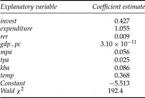
The estimates obtained from the HT model are shown in table 2. The overall fit is exceptionally good given the high significance of the Wald statistic (the associated p-value is close to 0). All coefficients are significant at the 1 per cent level and have the expected positive sign. In addition, a standard Lagrange multiplier (LM) test is performed to determine whether or not the environmental variables may be excluded from the model and this is rejected outright (p-value close to 0). This provides ample evidence that the environmental variables are properly included in the model in that they add significantly to the explanation of tourism demand.

Table 2.

Hausman–Taylor estimates

Note: All variables and Wald statistics significant at the 1% level.

A Hausman test is performed to determine if the HT model is to be preferred to the RE model and it pronounces clearly in favor of the HT model: the associated χ² statistic has a value of 22.2 and an associated p-value of 0.002. For completeness, the HT results are compared with those of a within (FE) estimator and the former is shown to be efficient relative to the latter (χ² value of 1.63 and an associated p-value of 95 per cent).

It is interesting to provide some interpretation to the results obtained. Policies aiming at protection of the biodiversity stock will positively impact tourism arrivals. Deterioration of the marine protected areas by 1 per cent, the terrestrial protected areas by 1 per cent and the key biodiversity sites by one site will result in a fall of 5.6 per cent, 2.5 per cent and 8.6 per cent, respectively, in tourist arrivals. This is not at all negligible for policy-making purposes. In the case of the more traditional economic variables, an increase (decrease) of US$ 1 billion of government expenditure and capital investment in the tourism sector (at constant 2000 prices), respectively, results in a 106 per cent and a 43 per cent increase (decrease) in tourist arrivals, which translates into a 11 per cent and 4 per cent increase (decrease) for an increase (decrease) of US$ 100 million (at constant 2000 prices). This is a relatively large amount of expenditure for the given impact on tourist arrivals and must be compared to the cost of preventing the deterioration of the environmental assets for an approximately similar impact. In addition, a unit appreciation in the real exchange rate (in domestic currency) leads to approximately 1 per cent decrease in arrivals.

It is clear, therefore, that while the traditional economic policy levers do have an effect on the demand for tourism in SIDS, the biodiversity factors are perhaps just as important, if not more important, and could very well become even more important in the future as a more environmentally conscious tourist develops in the richer countries of the world, where the bulk of tourists to SIDS originate.

These results for the coefficients of the economic variables are in line with both economic theory and other empirical findings in the literature. While results in the literature seem to vary widely from one study to the next (Eilat and Einav, Reference Eilat and Einav2004), expected relationships in terms of sign of coefficients are generally realized (for example Eilat and Einav, Reference Eilat and Einav2004; Eugenio-Martin et al., Reference Eugenio-Martin, Morales and Scarpa2004; Zhang and Jensen, Reference Zhang and Jensen2005; Naudé and Saayman, Reference Naudé and Saayman2005; Garin-Munoz, Reference Garin-Munoz2006). One interesting departure is that, while Eilat and Einav (Reference Eilat and Einav2004) found exchange rate variables to matter less to tourism arrivals in developing countries, our model which solely consists of developing countries found the real exchange rate to significantly affect it. For the few empirical papers that did consider biodiversity-related factors as explanatory variables to tourism demand, expected positive relationships were also found (Freytag and Vietze, Reference Freytag and Vietze2009; Loureiro et al., Reference Loureiro, Macagno, Nunes and Tol2012).