1. Introduction
Internal natural convection in a horizontal layer of a porous medium uniformly heated from below has been broadly investigated by many authors. The simplest case of convection in a homogeneous porous medium was first considered by Horton & Rogers (Reference Horton and Rogers1945) and independently by Lapwood (Reference Lapwood1948), who determined the critical Rayleigh (Rayleigh–Darcy) number,  ${\textit {Ra}}_c=4{\rm \pi}^2$, in the case of the isothermal and impermeable boundaries of the layer. The analysis was extended to other boundary conditions by Nield (Reference Nield1968). Afterwards, this Horton–Rogers–Lapwood (HRL) problem was considered, accounting for additional physical processes, including convection in anisotropic media (Epherre Reference Epherre1975), non-Darcy flow (Walker & Homsy Reference Walker and Homsy1977), hydrodynamic dispersion of temperature (Kvernvold & Tyvand Reference Kvernvold and Tyvand1980), nonlinear effects (Rees, Magyari & Keller Reference Rees, Magyari and Keller2005), viscous dissipation (Magyari, Rees & Keller Reference Magyari, Rees, Keller and Vafai2005) and other phenomena, which have been reviewed by Nield & Bejan (Reference Nield and Bejan2017).
Significant attention has been concentrated on convection in porous media considering local thermal non-equilibrium (LTNE), as reviewed by Straughan (Reference Straughan2015). Darcy–Bénard convection was studied by Banu & Rees (Reference Banu and Rees2002) and Postelnicu & Rees (Reference Postelnicu and Rees2003) for the case when the thermal equilibrium between the skeleton of the porous medium and the fluid breaks down, and these two solid and fluid phases have different temperatures. Using a two-temperature model, they showed that LTNE influences the onset of convection. A more general case of convection in bi-dispersed porous medium (BDPM) has received attention from Nield & Kuznetsov (Reference Nield and Kuznetsov2006) and Straughan (Reference Straughan2009). The BDPM is a standard porous medium in which the solid phase is replaced with another porous medium (Chen, Cheng & Zhao Reference Chen, Cheng and Zhao2000). Thus, there are macropores in the first medium and micropores in the second medium, which is nested in the first one. Both media have their own temperatures and fluid velocities. It was found that the critical Rayleigh number in BDPM can be much larger than that in the equivalent homogeneous porous medium. Recently, this study was extended by Straughan (Reference Straughan2018, Reference Straughan2019) to the case of anisotropic BDPM.
Understanding and predicting convection in BDPM is of interest for microfluidic applications related to designing heat transfer and insulation in small devices (Straughan Reference Straughan2015), as well as for flows over much larger space scales in geophysical applications. For example, convection in naturally fractured rocks has implications for geothermal energy extraction (Gérard et al. Reference Gérard, Genter, Kohl, Lutz, Rose and Rummel2006; Nie et al. Reference Nie, Meng, Jia, Zhang, Yang and Niu2012), ore deposits (Weis Reference Weis2015; Afanasyev et al. Reference Afanasyev, Blundy, Melnik and Sparks2018) and other transport processes in the Earth's crust (Simmons Reference Simmons2005). The dual-porosity dual-permeability model is a standard model for predicting fluid and heat transport in fractured rocks, although other approaches exist (Dietrich et al. Reference Dietrich, Helmig, Sauter, Teutsch, Hötzl and Köngeter2005). As for BDPM, such a model is built on the double-continuum concept by assuming the existence of two nested porous media, namely, the fractures, corresponding to the macropores, and the lower-permeability matrix blocks between the fractures corresponding to the micropores (Barenblatt, Zheltov & Kochina Reference Barenblatt, Zheltov and Kochina1960; Warren & Root Reference Warren and Root1963). The size of the matrix blocks can significantly exceed tens of metres in geologic reservoirs, which drastically increases the time required for pressure and temperature equilibration between the media. In many cases, natural flow in subsurface reservoirs is very slow. It can be simulated by employing Darcy's law, with the mass transfer between fractures and matrix driven by the difference in pressures, and the conduction heat transfer driven by the difference in temperatures (Pruess Reference Pruess1983; Pruess & Narasimhan Reference Pruess and Narasimhan1985). Thus, the governing equations for BDPM differ from those for the dual-porosity dual-permeability medium (DPM). The BDPM model usually accounts for the Brinkman term and momentum transfer between the media and neglects the fluid transport associated with different pressures in the fractures and the matrix. On the contrary, the DPM model accounts for the latter but assumes Darcy flow without accounting explicitly for the momentum transfer. Thus, the existing works on convection in BDPM cannot be directly applied to hydrothermal systems composed of naturally fractured rocks.
Hydrothermal fluid circulation through naturally fractured rocks exhibits a rich variety of flow patterns that have been widely investigated by means of the numerical modelling of Darcy flow. Yang, Latychev & Edwards (Reference Yang, Latychev and Edwards1998) and Diersch & Kolditz (Reference Diersch and Kolditz2002) showed that convection patterns in fractured-porous media differ from those in homogeneous media because fractures represent preferential pathways for fluid flow. The flow patterns of free convection were investigated by Simmons, Sharp & Nield (Reference Simmons, Sharp and Nield2008). It was shown that there can arise both intra-fracture convection patterns, i.e. when convection cells are parallel to fracture planes, and inter-fracture patterns, when convection cells are perpendicular to the fracture plane. Every convection cell is located in a single fracture in the case of intra-fracture patterns, whereas the cells are stretched over a pair of fractures in the case of inter-fracture patterns. Simmons et al. (Reference Simmons, Sharp and Nield2008) stress that both these modes must be taken into account to avoid underestimating the likelihood of convection. Recently, these and other patterns were simulated by Vujević et al. (Reference Vujević, Graf, Simmons and Werner2014) and Vujević & Graf (Reference Vujević and Graf2015). They considered different types of fracture networks and investigated how the network parameters influence the onset of convection and the flow patterns. It was found that the existence of regular fracture circuits lead to the onset of inter-fracture convection. Also, counter-rotating circulation cells can develop in nearby fractures.
The theoretical analysis, which to some extent can be applied for estimating the critical Rayleigh number in DPM, was conducted by McKibbin & O'Sullivan (Reference McKibbin and O'Sullivan1980). They considered the Darcy–Bénard convection in the case of a layered porous medium when particular layers, which are thin and characterized by high permeability, are considered fractures (McKibbin & Tyvand Reference McKibbin and Tyvand1984). The study by Banu & Rees (Reference Banu and Rees2002) can be applied to the convection in a dual-porosity (not dual-permeability) medium when the flow occurs only through fractures. To date, there has been no theoretical analysis of convection patterns in DPM, particularly in the case of dual permeability when fluid flow through each of the media and between them is possible. In addition to the noted practical significance, such an analysis would be useful for the better classification of the flow regimes simulated by Vujević et al. (Reference Vujević, Graf, Simmons and Werner2014) and others.
In this theoretical study, we analyse the flow patterns in the fractured-porous medium by considering the HRL problem for DPM. We examine the symmetric case of isothermal upper and lower boundaries of the layer when the respective spectral problem admits a relatively simple analytical solution and leave the cases of other boundary conditions for later studies. We investigate the critical Rayleigh number dependence upon similarity parameters and support analytical findings with numerical modelling of the convection flow. With a certain degree of approximation, the considered problem can be applied for understanding convective flows in a horizontal layer of a hydrothermal system bounded from above and below with impermeable rocks. We investigate the parameters leading to the onset of convection in such a layer and show that nine flow regimes can be established, depending on the parameters of the layer.
2. Problem statement
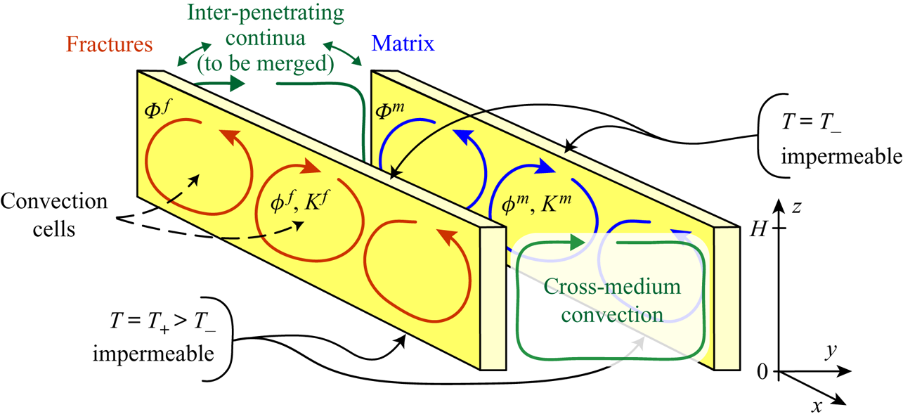
Let us consider an infinite horizontal layer of DPM of height  $H$ saturated with a single-phase fluid (figure 1,
 $x,y\in (-\infty ,\infty )$). Both the lower and upper boundaries of the layer are impermeable and isothermal, i.e. constant temperatures
 $T_+$ and
 $T_-=0$ are held at
 $z=0$ and
 $z=H$, respectively. It is assumed that the layer is uniformly heated from below, and so,
 $T_+ > T_-$.
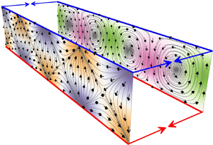
Sketch of the horizontal layer of DPM, which is modelled with two inter-penetrating continua  $\Phi ^{\,f}$ and
 $\Phi ^m$. For clarity, the layers corresponding to each continuum are drawn separately.

Applying the multi-continuum approach, we model convection in the fractured-porous medium using two inter-penetrating porous media (figure 1). The first medium,  $\Phi ^{\,f}$, corresponds to fractures, fissures or channels, forming high-permeability pathways for fluid, whereas the second medium,
 $\Phi ^m$, corresponds to low-permeability matrix blocks between the fractures. In what follows, we denote the parameters of fractures and matrix with the superscripts
 $f$ and
 $m$, respectively. Furthermore, we will not refer to
 $\Phi ^{\,f}$ and
 $\Phi ^m$ as ‘fractures’ and ‘matrix’ because the study may include a wider range of applications in which
 $\Phi ^{\,f}$ and
 $\Phi ^m$ correspond to different types of pore space.
We characterize the pore space of DPM with the relative volume  $\gamma =V^{\,f}/V$ of the medium
 $\Phi ^{\,f}$, where
 $V=V^{\,f}+V^m$ is the bulk representative elementary volume of DPM, and
 $V^{\,j}$,
 $j=f,m$ is the elementary volume occupied by
 $\Phi ^{\,j}$. Then, the relative volume of the medium
 $\Phi ^m$ is
 $1-\gamma =V^m/V$. We characterize each medium with its own porosity,
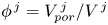 $\phi^{\,j}=V^{\,j}_{por}/V^{\,j}$, and absolute permeability,
 $K^{\,j}$, where
 $V^{\,j}_{por}$ is the volume of pore space in the corresponding medium. Then, the pore spaces of
 $\Phi ^{\,f}$ and
 $\Phi ^m$ occupy the fractions
 $\gamma \phi^{\,f}$ and
 $(1-\gamma )\phi ^m$ of the elementary volume
 $V$.
For the mathematical modelling of the natural convection, we formulate for each medium its own Darcy's law, along with the mass and energy balance equations. Furthermore, we investigate convection in the Oberbeck–Boussinesq approximation, and we thus account for the fluid density changes only in the terms containing the gravity acceleration  $\boldsymbol {g}$. The system of governing equations, which can be derived from Pruess (Reference Pruess1983), Pruess & Narasimhan (Reference Pruess and Narasimhan1985) and Dietrich et al. (Reference Dietrich, Helmig, Sauter, Teutsch, Hötzl and Köngeter2005), consists of
 \begin{gather} \displaystyle\rho^{\,j} = \rho_0 (1-\beta T^{\,j}),\quad j = f,m, \end{gather}
 \begin{gather} \displaystyle\boldsymbol{u}^{\,j} =- \frac{K^{\,j}}{\mu} (\nabla p^{\,j} -\rho^{\,j} \boldsymbol{g}),\end{gather}
 \begin{gather} \displaystyle\boldsymbol{\nabla}\boldsymbol{\cdot}\boldsymbol{u}^{\,j} = -b^{\,j} q^{\,fm}, \quad q^{\,fm}=\sigma_1 \frac{K^{m}}{\mu} (p^{\,f} - p^m), \end{gather}
 \begin{align} &(\rho c)^{\,j} \partial_t T^{\,j} + \boldsymbol{\nabla}\boldsymbol{\cdot} (\rho_0 c T^{\,j} \boldsymbol{u}^{\,j}) + \boldsymbol{\nabla}\boldsymbol{\cdot} (p^{\,j} \boldsymbol{u}^{\,j})\nonumber\\ &\quad= \rho^{\,j} \boldsymbol{g}\boldsymbol{\cdot} \boldsymbol{u}^{\,j} + \lambda^{\,j} \nabla^2 T^{\,j} - b^{\,j} q^{\,fm} (\rho_0 c T^{\,fm}+ p^{\,j}) - b^{\,j} \sigma_2 \lambda^{m} (T^{\,f} - T^m), \end{align}
where  $\rho$,
 $\mu$ and
 $\beta =\mbox {const}$ are the fluid density, the dynamic viscosity and the thermal expansion coefficient, respectively;
 $\rho _0$ is the reference value of the fluid density;
 $\boldsymbol {u}$ is the Darcy velocity;
 $p$ is the pressure;
 $T$ is the temperature;
 $q^{\,fm}$ is the mass flux from
 $\Phi ^{\,f}$ into
 $\Phi ^m$;
 $b^{\,f} = 1$ and
 $b^m = -1$ are constants;
 $\lambda ^{\,j}$ is the bulk heat conductivity of saturated medium
 $\Phi ^{\,j}$; and
 $(\rho c)^{\,j}$ is the bulk volume heat capacity of
 $\Phi ^{\,j}$, expressed as
 \[ (\rho c)^{\,f} = \gamma(\phi^{\,f} \rho_0 c +(1-\phi^{\,f}) \rho_r c_r), \quad (\rho c)^m = (1- \gamma) (\phi^m \rho_0 c +(1-\phi^m) \rho_r c_r). \]
Here, the subscript  $r$ denotes the parameters of the solid phase, which are assumed to be equal in both media, and
 $c$ and
 $c_r$ are the specific heat capacities of the fluid and solid phase, respectively.
Equation (2.1) is the fluid equation of state, (2.2) is Darcy's law and (2.3a) and (2.4) are the mass and energy balance equations for each medium. In (2.4), the terms  $\boldsymbol {\nabla }\boldsymbol {\cdot }(p^{\,j} \boldsymbol {u}^{\,j})$ and
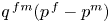 $q^{\,fm}(p^{\,f}-p^m)$, obtained by summing (2.4) for
 $j=f$ and
 $m$, correspond to the work of pressure when the fluid flows through each medium and between the media, respectively (Brownell, Garg & Pritchett Reference Brownell, Garg and Pritchett1977; Garg & Pritchett Reference Garg and Pritchett1977); the term
 $\rho ^{\,j} \boldsymbol {g}\cdot \boldsymbol {u}^{\,j}$ is the work of gravity;
 $\lambda ^{\,j} \nabla ^2 T^{\,j}$ corresponds to conductive heat transfer through each medium; and
 $q^{\,fm} \rho _0 c T^{\,fm}$ and
 $\sigma _2 \lambda ^{m} (T^{\,f} - T^m)$ are the convective and conductive heat transfers from
 $\Phi ^{\,f}$ to
 $\Phi ^m$. Here,
 $T^{\,fm}$ is the upwind value of temperature. If the fluid flows from
 $\Phi ^{\,f}$ into
 $\Phi ^m$ (
 $q^{\,fm}>0$), then
 $T^{\,fm} = T^{\,f}$, or vice versa; if it flows from
 $\Phi ^m$ into
 $\Phi ^{\,f}$ (
 $q^{\,fm}<0$), then
 $T^{\,fm} = T^m$. The definition of
 $T^{\,fm}$ is irrelevant in the linear perturbation analysis carried out in §§ 4–7 but is used in the numerical modelling of fluid transport presented in § 8. For further clarification of the energy balance equation, we substitute (2.2) and (2.3a) into (2.4) thereby expressing it as
 \begin{align} &(\rho c)^{\,j} \partial_t T^{\,j} + \rho_0 c \boldsymbol{u}^{\,j}\boldsymbol{\cdot}\nabla T^{\,j} - \lambda^{\,j} \nabla^2 T^{\,j}\nonumber\\ &\quad= \mu(\boldsymbol{u}^{\,j})^2/K^{\,j} - b^{\,j} \rho_0 c q^{\,fm} (T^{\,fm} - T^{\,j}) - b^{\,j} \sigma_2 \lambda^{m} (T^{\,f} - T^m). \end{align}
Thus, the energy balance equation for each  $\Phi ^{\,j}$ is the usual advection–diffusion equation for temperature with a source term – i.e. the right-hand side of (2.5) – equal to the sum of a dissipation term
 $\mu (\boldsymbol {u}^{\,j})^2/K^{\,j}$ (Ene & Sanchez-Palencia Reference Ene and Sanchez-Palencia1982) and the convective and conductive heat fluxes between
 $\Phi ^{\,j}$. The quadratic term
 $\mu (\boldsymbol {u}^{\,j})^2/K^{\,j}$ is the consequence of including the works of pressure and gravity in the energy balance (2.4). If one of the works is neglected and the other one is taken into account, then the dissipation term is not quadratic, and the dissipation can become negative. The governing equations thus contradict the second law of thermodynamics (Afanas'ev Reference Afanas'ev2012). Therefore, both works must be either taken into account or neglected. For generality of this study, we include both works in (2.4).
The mass flux and the conductive heat flux between the media,  $q^{\,fm}$ and
 $\sigma _2 \lambda ^{m} (T^{\,f} - T^m)$, respectively, are proportional to the products
 $\sigma _1K^m/\mu$ and
 $\sigma _2\lambda ^m$, which are the coefficients of mass and heat transfer between
 $\Phi ^{\,j}$. Here,
 $\sigma _1$ and
 $\sigma _2$ are the shape factors characterizing the fracture network. The constants
 $\sigma _1$ and
 $\sigma _2$ can be derived under the assumption of either quasi-steady (Warren & Root Reference Warren and Root1963; Kazemi et al. Reference Kazemi, Merrill, Porterfield and Zeman1976) or transient (Pruess & Narasimhan Reference Pruess and Narasimhan1985; Lim & Aziz Reference Lim and Aziz1995) exchange between
 $\Phi ^{\,j}$. Independently of the exchange model, we further consider
 $\sigma _1$ and
 $\sigma _2$ as given parameters. The transfer coefficients
 $\sigma _1K^m/\mu$ and
 $\sigma _2\lambda ^m$ are proportional to
 $K^m$ and
 $\lambda ^m$, reflecting that the mass and heat exchange between
 $\Phi ^{\,j}$ is mostly defined by the permeability and heat conductivity in
 $\Phi ^m$. In applications,
 $\sigma _1$ cannot be equal to
 $\sigma _2$. For example,
 $\sigma _1$ can be reduced by solute precipitation on the fracture walls and associated local permeability reduction. Similarly, in microfluidic applications,
 $\sigma _2$ can be reduced by designing DPM with insulated layers on the boundaries of high-permeability channels. However, in §§ 6–8, for simplicity, we restrict the study to the case of
 \begin{equation} \sigma_1\equiv\sigma_2. \end{equation}
The bulk parameters of DPM are expressed as
 \begin{equation} \left.\begin{array}{cc@{}} \overline{\phi} = \gamma \phi^{\,f}+ (1-\gamma)\phi^m, & \overline{K} = K^{\,f}+K^m,\\ \overline{(\rho c)} = (\rho c)^{\,f} + (\rho c)^m, & \overline{\lambda} = \lambda^{\,f}+\lambda^m, \end{array}\right\} \end{equation}
where, and in what follows, the bar denotes bulk quantities. These are the parameters of the homogeneous porous medium (EPM), which is equivalent to DPM under local equilibrium,  $p^{\,f}=p^m$ and
 $T^{\,f}=T^m$. If we sum (2.2)–(2.4) pairwise for
 $j=f$ and
 $m$ and place
 $p^{\,f}=p^m$ and
 $T^{\,f}=T^m$, then we obtain the equations for transport in EPM with the bulk parameters (2.7).
We assume that the system is in the conduction state. Thus, the basic steady-state solution represents the hydrostatic fluid distribution under local equilibrium between  $\Phi ^{\,j}$
 \begin{equation} T^{\,j} = T_+ -\alpha_0 z, \quad \boldsymbol{u}^{\,j} = 0, \end{equation}
where  $\alpha _0 = (T_+ - T_-)/H >0$ is constant. In the state (2.8), the porous medium is saturated with quiescent thermally stratified fluid.
The basic solution (2.8) satisfies the following boundary conditions:
 \begin{equation} \left.\begin{array}{ccc@{}} T^{\,j}=T_+, & u_z^{\,j} =0 & \mbox{on} \ z =0,\\ T^{\,j}=T_-, & u_z^{\,j} =0 & \mbox{on} \ z =H, \end{array}\right\} \end{equation}
corresponding to the isothermal and impermeable lower and upper boundaries of the layer. Here,  $u_z$ is the vertical component of fluid velocity.
3. Governing equations in dimensionless form
We take the layer thickness  $H$ as the characteristic length scale and denote the characteristic scales of the other parameters by the subscript
 $s$
 \begin{gather*} \rho_s = \rho_0 \alpha_0 \beta H, \quad p_s=\rho_s g H, \quad u_s = \frac{\overline{K}}{\mu} \rho_s g,\\ t_s=\frac{H \overline{\phi}}{u_s} = \frac{H \overline{\phi} \mu}{\overline{K} \rho_s g},\quad T_s = T_+ - T_- = \alpha_0 H. \end{gather*}
According to (2.1) and (2.8a), the density scale  $\rho _s$ is the fluid density change across the layer in the steady-state solution (2.8). Thus, the pressure scale
 $p_s$ is the increase in hydrostatic pressure head of height
 $H$ if the temperature at each point of the layer decreases by
 $T_s$. The scale
 $u_s$ is the instant Darcy velocity of a representative elementary volume of fluid heated up to the temperature
 $T_+$ and placed in the equivalent homogeneous layer of uniform temperature
 $T_-$, and
 $t_s$ is the time required for this volume to float up across the layer, assuming no heat exchange between the volume and the solid phase or other fluid.
Using the characteristic scales, we introduce the dimensionless parameters as
 \begin{equation} \boldsymbol{r}_* = \frac{\boldsymbol{r}}{H}, \quad \upsilon_* = \frac{\upsilon}{\upsilon_s},\quad \boldsymbol{r}=(x,y,z), \quad \upsilon = (\rho, p, T, u, t ), \end{equation}
where the asterisks denote the dimensionless variables, and  $\boldsymbol {r}$ is the position vector.
After substituting (2.7) and (3.1) into (2.1)–(2.4) and further omitting the asterisks of the dimensionless parameters, we obtain
 \begin{equation} \left.\begin{array}{c@{}} \displaystyle \rho^{\,j} = \alpha^{-1} - T^{\,j},\quad\boldsymbol{u}^{\,j} = - \kappa^{\,j} (\nabla p^{\,j} + \rho^{\,j}\boldsymbol{e}_z), \\ \displaystyle\boldsymbol{\nabla}\boldsymbol{\cdot}\boldsymbol{u}^{\,j} = - b^{\,j} q^{\,fm},\quad q^{\,fm}=\dfrac{\kappa^{m}}{B_1} (p^{\,f} - p^m), \\ \displaystyle S^{\,j} \partial_t T^{\,j} +\boldsymbol{u}^{\,j}\boldsymbol{\cdot}\nabla T^{\,j} + \Upsilon \boldsymbol{u}^{\,j}\boldsymbol{\cdot}\nabla p^{\,j} = - \Upsilon\rho^{\,j}\boldsymbol{u}^{\,j}\boldsymbol{\cdot}\boldsymbol{e}_z+\dfrac{\kappa^{\,j}}{{\textit{Ra}}^{\,j}} \nabla^2 T^{\,j} \\ \displaystyle \qquad\qquad\qquad\qquad\qquad\qquad- b^{\,j}q^{\,fm}(T^{\,fm}-T^{\,j}) - \dfrac{b^{\,j}\Lambda^{m}}{\overline{{\textit{Ra}}}B_2} (T^{\,f} -T^m), \end{array}\right\} \end{equation}
where  $\boldsymbol {e}_z$ is the unit vector in the opposite direction to gravity (
 $\boldsymbol {g}=-g\boldsymbol {e}_z$), and the following dimensionless quantities are introduced:
 \begin{equation} \left.\begin{array}{c@{}} \displaystyle S^{\,j} = \dfrac{(\rho c)^{\,j}}{\overline{\phi} \rho_0 c}, \quad {\textit{Ra}}^{\,j} = \dfrac{\rho_0^2 c K^{\,j} g H \alpha}{\lambda^{\,j} \mu}, \quad \overline{{\textit{Ra}}} = \dfrac{\rho_0^2 c \overline{K} g H \alpha}{\overline{\lambda} \mu},\quad \Upsilon=\dfrac{g \beta H}{c},\\ \displaystyle \alpha=\alpha_0 \beta H = \dfrac{\rho_s}{\rho_0}, \quad \kappa^{\,j} = \dfrac{K^{\,j}}{\overline{K}}, \quad\Lambda^{\,j} = \dfrac{\lambda^{\,j}}{\overline{\lambda}},\quad B_i=\dfrac{1}{\sigma_i H^2},\quad i=1,2. \end{array}\right\} \end{equation}
According to (3.3), the inequalities  $S^{\,j}>0$,
 ${\textit {Ra}}^{\,j}>0$, and
 $\overline {{\textit {Ra}}}>0$ hold, where
 ${\textit {Ra}}^{\,j}$ is the Rayleigh number for the medium
 $\Phi ^{\,j}$. The quantities
 $S^{\,j}$ and
 ${\textit {Ra}}^{\,j}$ for
 $\Phi ^{\,j}$ are related to
 $\overline {S}$ and
 $\overline {{\textit {Ra}}}$ for EPM by
 \begin{equation} \overline{S} = S^{\,f}+S^m, \quad \frac{1}{\overline{{\textit{Ra}}}} =\frac{\kappa^{\,f}}{{\textit{Ra}}^{\,f}} + \frac{\kappa^m}{{\textit{Ra}}^m}, \quad \overline{{\textit{Ra}}}=\Lambda^{\,f}{\textit{Ra}}^{\,f}+\Lambda^m{\textit{Ra}}^m, \end{equation}
where, according to the definitions of  $\kappa ^{\,j}$,
 $\Lambda ^{\,j}$, and
 ${\textit {Ra}}^{\,j}$ in (3.3), both expressions for
 $\overline {{\textit {Ra}}}$ can be applied at the same time.
The ratios  $\kappa ^{\,j}$ and
 $\Lambda ^{\,j}$ characterize the permeability and heat conductivity distribution between the two media, where
 $\kappa ^{\,f} + \kappa ^m = 1$ and
 $\Lambda ^{\,f} + \Lambda ^m = 1$. The fractions
 $\kappa ^{\,f}$ and
 $\Lambda ^{\,f}$ of the bulk quantities
 $\overline {K}$ and
 $\overline {\lambda }$ belong to
 $\Phi ^{\,f}$, whereas the fractions
 $\kappa ^m$ and
 $\Lambda ^m$ belong to
 $\Phi ^m$. The parameters
 $K^{\,j}$ and
 $\lambda ^{\,j}$ can vary in a wide range, depending on the particular porous medium. For example,
 $\lambda ^{\,j}$ depends on the heat conductivities of the solid and fluid phases, as well as the topology of the pore space, which can lead to either parallel or series transmission of heat (Ghanbarian & Daigle Reference Ghanbarian and Daigle2016). The permeability
 $K^{\,j}$ can also vary in a wide range depending on the topology of the pore space and the fracture density. The fracture permeability
 $K^{\,f}$ can be both larger and less than
 $K^m$ because it is proportional to the volumetric flux density
 $\boldsymbol {u}^{\,f}$ (Nield & Bejan Reference Nield and Bejan2017). The case of
 $K^{\,f}<K^m$ corresponds to
 $\gamma \ll 1$ when
 $|\boldsymbol {u}^{\,f}|<|\boldsymbol {u}^m|$ even though the intrinsic average velocity in
 $\Phi ^{\,f}$ can be larger than that in
 $\Phi ^m$, i.e.
 $|\boldsymbol {u}^{\,f}|/\gamma \phi^{\,f}>|\boldsymbol {u}^m|/(1-\gamma )\phi ^m$. To account for all types of porous medium, we assume
 $0\leq \kappa ^{\,j}\leq 1$ and
 $0\leq \Lambda ^{\,j}\leq 1$.
The quantities  $B_i$ characterize the intensity of mass and heat transfer between
 $\Phi ^{\,j}$. If
 $B_i\ll 1$, then the flow occurs under local equilibrium and one can use EPM as a substitute for DPM. If
 $B_i\sim 1$ or
 $B_i \gg 1$, then the local equilibrium breaks down and one must apply DPM in order to account for different pressures and temperatures in
 $\Phi ^{\,j}$. In geophysical applications, the shape factors
 $\sigma _i$ can be estimated as
 $\sigma _i=d/L_b^2$, where
 $L_b$ is the characteristic distance between fractures, and typically, the constant
 $d$ lies in the range of 4–27 (Kazemi et al. Reference Kazemi, Merrill, Porterfield and Zeman1976; Lim & Aziz Reference Lim and Aziz1995). The double-continuum concept is meaningful if
 $L_b\ll H$, i.e. if a representative elementary volume in
 $\Phi ^{\,f}$ can be defined for volume averaging (Dietrich et al. Reference Dietrich, Helmig, Sauter, Teutsch, Hötzl and Köngeter2005). The relation
 $L_b\ll H$ is equivalent to
 $B_i\ll 1$. As noted above, particular physical phenomena, e.g. local permeability reduction due to solute precipitation, can increase
 $B_i$, but we bear in mind that
 $B_i>1$ is unlikely in a geophysical context. In a designed porous medium, e.g. if
 $\Phi ^{\,f}$ corresponds to channels embedded into a low-permeability medium, the meaningful values of
 $B_i$ can be higher than1. For convection in BDPM, Nield & Kuznetsov (Reference Nield and Kuznetsov2006) consider
 $B_2$ in the range of 0–100. Further, we investigate convection regimes at
 $0\le B_i\le 100$,
 $0\leq \kappa ^{\,j}\leq 1$, and
 $0\leq \Lambda ^{\,j}\leq 1$ so as not to miss any application.
Substituting (2.1) and (2.2) into (2.8b) and integrating the obtained equation, we reduce (2.8) and (2.9) to the following dimensionless form:
 \begin{gather} p^{\,j}= 1-\frac{1-\alpha}{\alpha}z-\frac{z^2}{2}, \quad T^{\,j} = 1-z, \quad \rho^{\,j}=\frac{1-\alpha}{\alpha}+z, \end{gather}
 \begin{gather} \left. \begin{array}{lll} \displaystyle T^{\,j}=1, & u_z^{\,j} =0 & \mbox{on}\ z=0,\\ T^{\,j}=0, & u_z^{\,j} =0 & \mbox{on}\ z=1. \end{array}\right\}\end{gather}
4. Dispersion equation
4.1. Derivation of the equation
We now examine the stability of the basic solution (3.5) by substituting
 \begin{equation*} p^{\,j} = 1-\frac{1-\alpha}{\alpha}z-\frac{z^2}{2} + \Pi^{\,j}, \quad T^{\,j} = 1 - z+ \Theta^{\,j}, \quad \rho^{\,j}=\frac{1-\alpha}{\alpha}+z+R^{\,j}, \end{equation*}
into (3.2), where  $\Pi ^{\,j}, \Theta ^{\,j}, R^{\,j} (\boldsymbol {r}, t) \rightarrow 0$ are small perturbations of the
 $p$,
 $T$ and
 $\rho$. The fluid velocity is also assumed to be small,
 $\boldsymbol {u}^{\,j}\rightarrow 0$. After neglecting second-order small quantities and eliminating
 $q^{\,fm}$ between (3.2), we obtain the linearized equations
 \begin{gather} R^{\,j}=-\Theta^{\,j},\quad \boldsymbol{u}^{\,j} = - \kappa^{\,j} (\nabla \Pi^{\,j} +R^{\,j} \boldsymbol{e}_z ), \end{gather}
 \begin{gather} \left. \begin{array}{c@{}} \displaystyle \kappa^{\,j}\left(\nabla^2 \Pi^{\,j} - \nabla_z \Theta^{\,j}\right) = \dfrac{b^{\,j} \kappa^{m}}{ B_1} (\Pi^{\,f} - \Pi^m),\\ \displaystyle S^{\,j} \partial_t \Theta^{\,j} + \kappa^{\,j}(\nabla_z \Pi^{\,j} - \Theta^{\,j}) =\dfrac{\kappa^{\,j}}{{\textit{Ra}}^{\,j}} \nabla^2 \Theta^{\,j} - \dfrac{b^{\,j}\Lambda^{m}}{\overline{{\textit{Ra}}}B_2} (\Theta^{\,f} -\Theta^m), \end{array}\right\} \end{gather}
where (4.2) form a closed system of four linear partial differential equations for  $\Pi ^{\,j}$ and
 $\Theta ^{\,j}$, and the fluid densities and velocities can be expressed in terms of
 $\Pi ^{\,j}$ and
 $\Theta ^{\,j}$ using (4.1).
Separating the variables, we present the solution to (4.2) in the form
 \begin{equation} \Pi^{\,j} = \Pi_0^{\,j}(z) \zeta , \quad \Theta^{\,j} = \Theta_0^{\,j}(z) \zeta , \quad \zeta = \exp(\mathrm{i}(k_x x +k_y y) + \Omega t), \end{equation}
where  $k_x$ and
 $k_y$ are the wavenumbers and
 $\Omega$ is the growth rate. We assume that
 $k_x$ and
 $k_y$ are real numbers. This implies that the perturbations are not brought from infinity (
 $x, y \rightarrow \infty$), so the convection is not generated by an external force. Substituting (4.3) into (3.6) and (4.2), we obtain
 \begin{equation} \left. \begin{array}{c@{}} \displaystyle \kappa^{\,j}\left(\dfrac{\mathrm{d}^2\Pi_0^{\,j}}{\mathrm{d}z^2} - k_{xy}^2 \Pi_0^{\,j} - \dfrac{\mathrm{d}\Theta_0^{\,j}}{\mathrm{d}z}\right) - \dfrac{b^{\,j}\kappa^{m}}{B_1} (\Pi_0^{\,f} - \Pi_0^m) = 0, \\ \displaystyle \Omega S^{\,j} \Theta_0^{\,j} + \kappa^{\,j}\left(\dfrac{\mathrm{d}\Pi_0^{\,j}}{\mathrm{d}z} - \Theta_0^{\,j}\right) - \dfrac{\kappa^{\,j}}{{\textit{Ra}}^{\,j}} \left(\dfrac{\mathrm{d}^2\Theta_0^{\,j}}{\mathrm{d}z^2} - k_{xy}^2 \Theta_0^{\,j}\right) \\ \displaystyle \qquad\qquad\qquad\qquad\qquad\qquad\quad + \dfrac{b^{\,j}\Lambda^{m}}{\overline{{\textit{Ra}}}B_2} (\Theta_0^{\,f} - \Theta_0^m ) = 0, \end{array}\right\} \end{equation}
with the boundary conditions
 \begin{equation} \Theta_0^{\,j} = 0, \quad \frac{\mathrm{d}\Pi_0^{\,j}}{\mathrm{d}z} = 0\quad \mbox{on}\ z=0\quad \mbox{and}\quad z=1, \end{equation}
where 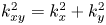 $k_{xy}^2 = k_x^2 + k_y^2$ denotes the overall horizontal wavenumber. Without loss of generality, we assume that
 $k_{xy}\geq 0$ because this wavenumber enters (4.4) only as
 $k_{xy}^2$.
A non-trivial solution to the eigenvalue problem given by (4.4) and (4.5) exists for particular values of the spectral parameter  $\Omega$. For boundary conditions considered in this paper (4.5), the non-trivial solution to the conjugate problem can be written in the following simple form (Davis Reference Davis1969):
 \begin{equation} \Theta_0^{\,j} = \delta \Theta^{\,j} \sin(k_z z),\quad \Pi_0^{\,j} =\delta \Pi^{\,j} \cos(k_z z), \quad k_z = {\rm \pi} n, \quad n=1,2,3,\ldots, \end{equation}
where  $k_z$ is a real number that takes discrete values, and the constant amplitudes
 $\delta \Pi ^{\,j}$ and
 $\delta \Theta ^{\,j}$ are still unknown. To determine
 $\delta \Pi ^{\,j}$ and
 $\delta \Theta ^{\,j}$, we substitute (4.6) into (4.4). This yields
 \begin{equation} \left. \begin{array}{c@{}} \displaystyle \left(k^2 \kappa^{\,j} + \dfrac{\kappa^{m}}{B_1}\right) \delta \Pi^{\,j} + k_z \kappa^{\,j} \delta \Theta^{\,j} - \dfrac{\kappa^{m}}{B_1} \delta \Pi^i = 0, \\ \displaystyle - k_z \kappa^{\,j} \delta \Pi^{\,j} + \left(\Omega S^{\,j} - \kappa^{\,j} +k^2\dfrac{\kappa^{\,j}}{{\textit{Ra}}^{\,j}} +\dfrac{\Lambda^{m}}{\overline{{\textit{Ra}}}B_2} \right) \delta \Theta^{\,j} - \dfrac{\Lambda^{m}}{\overline{{\textit{Ra}}}B_2}\delta \Theta^i = 0, \end{array} \right\} \end{equation}
where we introduce the notation 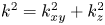 $k^2 = k_{xy}^2+k_z^2$ and
 $i=f,m$,
 $i\neq j$.
Equations (4.7) form a homogeneous system of linear equations with respect to  $\delta \Pi ^{\,j}$ and
 $\delta \Theta ^{\,j}$. There is a non-trivial solution if the matrix of coefficients for (4.7) is singular. By calculating and equating to zero the determinant of the matrix and carrying out identity transformations, we obtain the following dispersion relation:
 \begin{equation} D^{\,f}D^m+\left(D^{\,f}+D^m\right)Z^c = 0, \end{equation}
where we denote
 \begin{equation} D^{\,j} = \Omega S^{\,j} + \kappa^{\,j} \left( \frac{k^2}{{\textit{Ra}}^{\,j}} - \frac{k_{xy}^2}{k^2} \right), \quad Z^c = \frac{\Lambda^{m}}{\overline{{\textit{Ra}}}B_2} - \frac{\kappa^{\,f} \kappa^m}{k^2 \kappa^{\,f} B_1 + 1} \frac{k_z^2}{k^2}. \end{equation}
The equation  $D^{\,j} = 0$ is the dispersion relation in the HRL problem for the regular single porosity medium
 $\Phi ^{\,j}$, assuming zero mass and heat exchange with the adjacent medium.
Assuming that 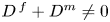 $D^{\,f}+D^m\neq 0$, (4.8) can be written as
 \begin{equation} \frac{D^{\,f} D^m}{D^{\,f} +D^m} =-Z^c. \end{equation}
The left-hand side of (4.10) is proportional to the harmonic mean of  $D^{\,j}$, reflecting that the mass and heat transfer through DPM occur in parallel through
 $\Phi ^{\,f}$ and
 $\Phi ^m$. This is analogous to parallel conductors (Nield & Simmons Reference Nield and Simmons2007).
Taking into account (4.8) and (4.9), we derive from (4.1) and (4.7) the following relationships for the amplitudes:
 \begin{gather} D^{\,f}\delta\Theta^{\,f}+D^m\delta\Theta^m=0, \end{gather}
 \begin{gather} \delta\Pi^{\,j}=\frac{1}{\kappa^{\,j}k_z}\left(-\frac{\kappa^{\,j}}{D^{\,j}}\frac{k_z^2}{k^2}-\frac{1}{Z^c}\left(\frac{\Lambda^{m}}{\overline{{\textit{Ra}}} B_2}-Z^c\right)\right)D^{\,j}\delta\Theta^{\,j}, \end{gather}
 \begin{gather} \left.\begin{array}{c@{}} \displaystyle \delta u^{\,j}_z=\left(\dfrac{\kappa^{\,j}}{D^{\,j}}\dfrac{k_{xy}^2}{k^2}-\dfrac{1}{Z^c}\left(\dfrac{\Lambda^{m}}{\overline{{\textit{Ra}}} B_2}-Z^c\right)\right)D^{\,j}\delta\Theta^{\,j}, \\ \displaystyle \delta q^{\,fm}=\dfrac{\kappa^{m}}{B_1}\left(\delta \Pi^{\,f}-\delta \Pi^m\right)=\dfrac{1}{Z^c}\left(\dfrac{\Lambda^{m}}{\overline{{\textit{Ra}}} B_2}-Z^c\right)D^{\,f}\delta\Theta^{\,f}, \end{array}\right\} \end{gather}
where  $\delta u^{\,j}_z$ and
 $\delta q^{\,fm}$ are the amplitudes of
 $u_z$ and
 $q^{\,fm}$ in the solution given by (4.3) and (4.6)
 \begin{equation} u^{\,j}_z=\delta u^{\,j}_z\sin(k_z z)\zeta,\quad q^{\,fm}=\delta q^{\,fm}\cos(k_z z)\zeta. \end{equation}
4.2. Geometric interpretation
In general, the growth rate  $\Omega$ is a complex number. According to (4.3), if
 $\textrm {Re}\,\Omega >0$, then the perturbation grows, and if
 $\textrm {Re}\,\Omega <0$, then it fades. From (4.9), it follows that (4.8) is a quadratic equation with respect to
 $\Omega$
 \begin{equation} a_0 \Omega^2 + a_1 \Omega + a_2 = 0, \end{equation}
which coefficients are given by
 \begin{gather} a_0 = S^{\,f}S^m, \quad a_1 = S^{\,f} Z^m + S^m Z^{\,f} + \overline{S} Z^c, \quad a_2 = Z^{\,f} Z^m + Z^{\,f} Z^c +Z^m Z^c, \end{gather}
 \begin{gather} Z^{\,j} = \kappa^{\,j} \left( \frac{k^2}{{\textit{Ra}}^{\,j}} - \frac{k_{xy}^2}{k^2} \right)=D^{\,j}-\Omega S^{\,j}, \quad j=f,m. \end{gather}
We apply the Routh–Hurwitz stability criterion to the characteristic polynomial (4.15) to determine the parameters corresponding to  $\textrm {Re}\,\Omega \leq 0$. The inequality
 $a_0>0$ holds because
 $S^{\,j} > 0$. Therefore, the thermal stratification is stable if and only if all leading principal minors of the Hurwitz matrix are positive. This leads to the inequalities
 $a_1\geq 0$ and
 $a_2\geq 0$, or using the notations of (4.16b,c), to
 \begin{equation} S^{\,f} Z^m + S^m Z^{\,f} + \overline{S} Z^c \geq 0,\quad Z^{\,f} Z^m +Z^{\,f} Z^c +Z^m Z^c \geq 0. \end{equation}
In the space 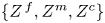 $\lbrace Z^{\,f}, Z^m, Z^c \rbrace$, the equations
 $a_1 = 0$ and
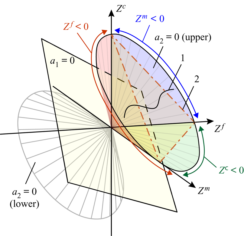
 $a_2 = 0$ define a plane and a circular conical surface, respectively (figure 2). The origin is the only point of intersection of these surfaces. Indeed, if we express
 $Z^c$ from the equation
 $a_1 = 0$ and substitute it into the equation
 $a_2=0$, then we obtain
 \[ (Z^{\,f})^2 S^m + (Z^m)^2 S^{\,f} = 0. \]
This equation is satisfied only if both  $Z^{\,f} = 0$ and
 $Z^m = 0$, and according to (4.16b,c),
 $Z^c = 0$. Thus, the plane
 $a_1=0$ splits the conical surface
 $a_2 = 0$ into the upper and lower parts, which contain the intervals
 $Z^c>0$ and
 $Z^c<0$ of the axis
 $Z^c$, respectively. The inequality
 $a_1\geq 0$ constrains the upper region above the plane, and the inequality
 $a_2\geq 0$ constrains the region inside the conical surface (figure 2). Therefore, the parameters of stable layers, in which convection does not occur, coincide with the interior of the upper conical surface given by (4.18). If
 $\overline {{\textit {Ra}}} \rightarrow 0$, then all solutions to (4.8) satisfy inequalities (4.18) because if the dimensional temperature gradient
 $\alpha _0$ approaches 0, then the thermal stratification is stable. This means that the locus of the solution for each
 $n =\mbox {const}$ is a curve lying inside the conical surface at
 $\overline {{\textit {Ra}}}\rightarrow 0$ (figure 2, curve 1). Each curve can be parameterized by either
 $k_{xy}$ or
 $\Omega$. With rising
 $\overline {{\textit {Ra}}}$, i.e. with increasing temperature gradient
 $\alpha _0$, one of these curves (further analysis of solutions to (4.8) shows that it is with
 $n=1$) approaches the boundary of (4.18b), and it first intersects the boundary at the critical Rayleigh number,
 $\overline {{\textit {Ra}}}_c$. If
 $\overline {{\textit {Ra}}} > \overline {{\textit {Ra}}}_c$, then a segment of such curve corresponding to growing perturbations lies outside the stability region (4.18). At
 $\overline {{\textit {Ra}}} =\overline {{\textit {Ra}}}_c$, the locus touches exactly the conical surface
 $a_2 = 0$ and not the plane surface
 $a_1 = 0$. Therefore, the inequality (4.18b) is more relevant than (4.18a) because it is this inequality that is violated at
 $\overline {{\textit {Ra}}} =\overline {{\textit {Ra}}}_c$. The critical number
 $\overline {{\textit {Ra}}}_c$ is the minimum
 $\overline {{\textit {Ra}}}$ for which the equation
 $a_2=0$ has a solution.
Sketch of the locus of solutions to the dispersion equation in the 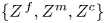 $\lbrace Z^{\,f}, Z^m, Z^c \rbrace$ space (curve 1) and key surfaces defining the onset of convection. The coordinate axes belong to the conical surface
 $a_2=0$.

According to (4.15) and (4.16), the monotonic (not oscillatory) instability of the basic state (3.6) develops at near-critical parameters,  $\overline {{\textit {Ra}}}\rightarrow \overline {{\textit {Ra}}}_c+$. This means that if
 $\textrm {Re}\,\Omega \rightarrow 0$ (or
 $a_2 \rightarrow 0$), then
 $\textrm {Im}\,\Omega \equiv 0$. Indeed, if
 $a_2 \rightarrow 0$, then the discriminant of (4.15) is not negative, and therefore, both solutions to (4.15) are real numbers.
5. Sufficient stability conditions
To assist interpretation of the numerical solutions to (4.8) presented in § 7, it is worth considering several asymptotic cases for (4.8) to explicitly show some not obvious features of the convection. For this reason, we present the sufficient stability conditions in § 5 and several particular solutions to (4.8) in § 6.
To satisfy (4.18), it is sufficient to satisfy the three more simple inequalities simultaneously for all  $k_x$,
 $k_y$ and
 $k_z$
 \begin{equation} Z^{\,f}\geq 0, \quad Z^m\geq 0,\quad Z^c\geq 0. \end{equation}
Therefore, these inequalities are sufficient conditions for stability of the stratification (3.6), i.e. for the absence of convection. The conditions (5.1) mean that parameters of all perturbations (4.3) in the  $\lbrace Z^{\,f}, Z^m, Z^c \rbrace$ space lie inside the conical surface for which the directrix is the triangle with vertices belonging to each of three coordinate axes (figure 2, surface 2). The geometrical interpretation of the sufficient conditions is as follows: if the locus of solutions to (4.8) lies inside that conical surface, then it also lies inside the circular conical surface
 $a_2 = 0$.
According to (4.17), the inequality  $Z^{\,j} \geq 0$ is identical to the following:
 \begin{equation} {\textit{Ra}}^{\,j} \leq k^4/k_{xy}^2. \end{equation}
To satisfy (5.2) for all  $k_x$,
 $k_y$ and
 $k_z$, one must determine those wavenumbers that minimize the right-hand side of (5.2) and set
 ${\textit {Ra}}^{\,j}$ less than that minimum. For every discrete value of
 $k_z = {\rm \pi} n$, the minimum
 $4 {\rm \pi} ^2 n^2$ of the
 $k^4 / k_{xy}^2$ ratio is reached at
 $k_{xy} = {\rm \pi} n$ (Horton & Rogers Reference Horton and Rogers1945). Therefore, if
 \begin{equation} {\textit{Ra}}^{\,j} \leq 4 {\rm \pi}^2 n^2, \end{equation}
then (5.2) holds for corresponding  $n$. The inequality (5.3) is identical to the stability condition for a homogeneous medium. Consequently, the sign of the quantity
 $Z^{\,f}$ (or
 $Z^m$) defines the stability of the basic state (3.5) in the medium
 $\Phi ^{\,f}$ (or
 $\Phi ^m$), if it is assumed to be isolated from the other medium
 $\Phi ^m$ (or
 $\Phi ^{\,f}$). If
 $Z^{\,j} \geq 0$ for all
 $k_x$,
 $k_y$ and
 $k_z = {\rm \pi} n$, then the conduction state in the isolated medium
 $\Phi ^{\,j}$ is stable, and if
 $Z^{\,j}<0$, then convection occurs.
According to (4.9b), the inequality  $Z^c\geq 0$ is identical to the following:
 \begin{equation} \overline{{\textit{Ra}}} \leq \frac{\Lambda^{m}(k^2\kappa^{\,f}B_1+1)}{\kappa^{\,f}\kappa^m B_2}\frac{k^2}{k_z^2}. \end{equation}
The right-hand side of (5.4) is the increasing function of  $k_{xy}^2$ (if
 $k_{xy}^2 \geq 0$); therefore, it reaches a minimum at
 $k_{xy}^2 = 0$. Consequently, inequality (5.4) for every
 $k_z = {\rm \pi} n$ reduces to
 \begin{equation} \overline{{\textit{Ra}}} \leq \frac{\Lambda^{m}({\rm \pi}^2 n^2\kappa^{\,f}B_1 + 1)}{\kappa^{\,f}\kappa^m B_2}. \end{equation}
If (5.5) holds, then the inequality  $Z^c\geq 0$ is satisfied for all
 $k_x$,
 $k_y$ and
 $k_z = {\rm \pi} n$.
The inequalities (5.3) and (5.5) are most restrictive for the first mode, i.e. if  $n=1$. In this case, the conditions (5.3) and (5.5) reduce to
 \begin{equation} {\textit{Ra}}^{\,j} \leq 4 {\rm \pi}^2, \quad \overline{{\textit{Ra}}} \leq \frac{\Lambda^{m}({\rm \pi}^2\kappa^{\,f}B_1 + 1)}{\kappa^{\,f}\kappa^mB_2}. \end{equation}
The simultaneous fulfilment of inequalities (5.6) is the sufficient condition for the absence of convection. The inequality (5.6a) means that both conduction states in isolated  $\Phi ^{\,f}$ and
 $\Phi ^m$ are stable; however, this does not guarantee stability for DPM. As shown in §§ 6.4 and 7, the intriguing observation is that, even if the states in
 $\Phi ^{\,j}$ are stable, the thermal stratification in DPM can be unstable to a perturbation such that
 $Z^{\,f}>0$,
 $Z^m>0$, and
 $Z^c<0$ (figure 2). It is sufficient to satisfy the inequality (5.6b) to guarantee the stability to all such perturbations.
6. Particular solutions to the dispersion equation
In what follows in §§ 6–8, we assume that (2.6) holds. Then, all parameters in the relations (4.9b) and (4.17) for  $Z^c$,
 $Z^{\,f}$ and
 $Z^m$ can be expressed by using only four dimensionless quantities –
 $\overline {{\textit {Ra}}}$,
 $\kappa$,
 $\Lambda$ and
 $B$
 \begin{equation} \left.\begin{array}{c@{}} \displaystyle \kappa^{\,f} \equiv\kappa, \quad \kappa^m = 1- \kappa,\quad \Lambda^{\,f} \equiv \Lambda, \quad \Lambda^m =1 - \Lambda, \\ \displaystyle B_1\equiv B_2\equiv B,\quad {\textit{Ra}}^{\,f} = \overline{{\textit{Ra}}}\dfrac{\kappa}{\Lambda}, \quad {\textit{Ra}}^m = \overline{{\textit{Ra}}}\dfrac{ 1 -\kappa}{1 - \Lambda}. \end{array}\right\} \end{equation}
Consequently,  $\overline {{\textit {Ra}}}_c$ depends only on
 $\kappa$,
 $\Lambda$ and
 $B$, according to the most restrictive condition (4.18b). Further, we investigate this dependence and associated flow regimes immediately above criticality at
 $\overline {{\textit {Ra}}}\rightarrow \overline {{\textit {Ra}}}_c+$. We investigate the dependence
 $\overline {{\textit {Ra}}}_c(\kappa , \Lambda , B)$ analytically in this section for particular asymptotic cases and numerically in § 7. We also assume that
 $n=1$ because for larger
 $n\geq 2$, the number
 $\overline {{\textit {Ra}}}_c$ is larger than that for
 $n=1$. This assumption is in agreement with the discussion in § 5, and it is also supported by the numerical solutions to (4.8).
6.1. Asymptotic  $B\rightarrow 0$

Let us consider the layer stability in the asymptotic case  $B\rightarrow 0$ corresponding to local equilibrium between
 $\Phi ^{\,j}$. If
 $B\rightarrow 0$, then according to (4.9b),
 $Z^c\rightarrow \infty$. Consequently, the dispersion equation (4.8) can be satisfied only if
 $D^{\,f}+D^m\rightarrow 0$ because
 $Z^{\,f}$ and
 $Z^m$ are independent of
 $B$. Substituting (3.4) and (4.9a) into the equation
 $D^{\,f}+D^m=0$, we obtain the dispersion relation at
 $B=0$
 \begin{equation} \Omega\overline{S}+\frac{k^2}{\overline{{\textit{Ra}}}}-\frac{k_{xy}^2}{k^2}=0. \end{equation}
This equation is the dispersion relation for EPM (Horton & Rogers Reference Horton and Rogers1945). Therefore, the conduction state (3.6) at  $B=0$ is stable at
 $\overline {{\textit {Ra}}}\leq 4{\rm \pi} ^2$ and unstable otherwise at
 $\overline {{\textit {Ra}}}>4{\rm \pi} ^2$. This yields
 \begin{equation} \overline{{\textit{Ra}}}_c\rightarrow4{\rm \pi}^2,\quad k_c\rightarrow{\rm \pi}\quad\mbox{as}\ B\rightarrow 0, \end{equation}
where  $k_c$ is the critical overall horizontal wavenumber
 $k_{xy}$. The relations (6.3) are the consequence of DPM equivalence to EPM in the case of local equilibrium at
 $B\rightarrow 0$.
6.2. Asymptotic $B\rightarrow \infty$

We now consider the system behaviour in the asymptotic case  $B\rightarrow \infty$ corresponding to infinite time required for reaching local equilibrium. Thus, the heat and mass exchange between
 $\Phi ^{\,j}$ are absent, and the media can be considered isolated from each other. The local equilibrium is never reached in the case of
 $B\rightarrow \infty$. As noted in § 3, a realistic porous medium cannot be characterized with large values of
 $B$, but from the mathematical point of view, the asymptotic
 $B\rightarrow \infty$ allows for simple conclusions to be reached that, as we will show, do extrapolate into the region of finite
 $B\sim 1$.
If  $B\rightarrow \infty$, then according to (4.9b),
 $Z^c\rightarrow 0$ and (4.8) reduces to
 \[ D^{\,f}D^m=0 \]
or according to (4.17), to
 \[ Z^{\,f}Z^m=0 \]
in the case of neutral stability ( $\Omega =0$). Thus, in the asymptotic case
 $B\rightarrow \infty$, the convection develops at the minimum
 $\overline {{\textit {Ra}}}$ for which either
 $Z^{\,f}=0$ or
 $Z^m=0$ is satisfied. If the condition
 $Z^{\,f}=0$ (or
 $Z^m=0$) is reached first with increasing
 $\overline {{\textit {Ra}}}$, then the state (3.6) in
 $\Phi ^{\,f}$ (or
 $\Phi ^m$) becomes unstable and convection appears in
 $\Phi ^{\,f}$ (or
 $\Phi ^m$). At the same time, the stratification in the adjacent medium
 $\Phi ^m$ (or
 $\Phi ^{\,f}$) remains stable. According to (5.3),
 $Z^{\,j}=0$ is satisfied if
 ${\textit {Ra}}^{\,j}={\textit {Ra}}^{\,j}_c=4{\rm \pi} ^2$ and
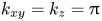 $k_{xy}=k_z={\rm \pi}$. Consequently, the following asymptotic relation holds:
 \begin{equation} \overline{{\textit{Ra}}}_c\rightarrow \min\left({\textit{Ra}}^{\,f}_c\frac{\Lambda^{\,f}}{\kappa^{\,f}},{\textit{Ra}}^m_c\frac{\Lambda^m}{\kappa^m}\right),\quad k_c\rightarrow{\rm \pi}\quad\mbox{as}\ B\rightarrow\infty. \end{equation}
Substituting (6.1) into (6.4) yields
 \begin{equation} \overline{{\textit{Ra}}}_c\rightarrow4{\rm \pi}^2 \min\left(\frac{\Lambda}{\kappa},\frac{1-\Lambda}{1-\kappa}\right)\leq 4{\rm \pi}^2\quad\mbox{as}\ B\rightarrow\infty. \end{equation}
The minimum of the fractions in (6.5) is not larger than unity for  $0\leq \kappa \leq 1$ and
 $0\leq \Lambda \leq 1$, and it reaches a maximum at
 $\kappa =\Lambda$, i.e. if
 $\overline {K}$ and
 $\overline {\lambda }$ are distributed in equal proportions between
 $\Phi ^{\,j}$. Then, according to (6.5),
 $\overline {{\textit {Ra}}}_c$ reaches the maximum value of
 $4{\rm \pi} ^2$ in the case of
 $\kappa =\Lambda$ as compared to other values of
 $\kappa$ and
 $\Lambda$. Therefore, we can conclude for
 $B\rightarrow \infty$ that
 $\overline {{\textit {Ra}}}_c$ for DPM does not exceed that for EPM. The onset of convection in DPM occurs for smaller (or equal at
 $\kappa =\Lambda$) vertical temperature gradients
 $\alpha _0$ than that in EPM.
If  $\kappa >\Lambda$, then the first fraction within the brackets in (6.5) is smaller than the second one, i.e. convection occurs in
 $\Phi ^{\,f}$ at
 $\overline {{\textit {Ra}}}\rightarrow \overline {{\textit {Ra}}}_c+$ (
 ${\textit {Ra}}^{\,f}_c=4{\rm \pi} ^2>{\textit {Ra}}^m_c$). If
 $\kappa <\Lambda$, then the second fraction in (6.5) is larger, i.e. convection occurs in
 $\Phi ^m$ (
 ${\textit {Ra}}^m_c=4{\rm \pi} ^2>{\textit {Ra}}^{\,f}_c$). Thus, we can expect that for any finite and sufficiently large
 $B$, where
 $\overline {{\textit {Ra}}}\rightarrow \overline {{\textit {Ra}}}_c+$, and
 $\kappa >\Lambda$ (or
 $\kappa <\Lambda$), the convection pattern in DPM is determined by the flow in the medium
 $\Phi ^{\,f}$ (or
 $\Phi ^m$) because it is the stratification in this medium that is unstable at
 $B\rightarrow \infty$.
6.3. Case $\kappa =\Lambda$

If  $\overline {K}$ and
 $\overline {\lambda }$ are distributed between
 $\Phi ^{\,f}$ and
 $\Phi ^m$ in equal proportions, i.e.
 $\kappa =\Lambda$, then we derive from (4.9b), (4.17), and (6.1)
 \begin{align} Z^{\,f}=\kappa\left(Z^{\,f}+Z^m\right),\quad Z^m=(1-\kappa)\left(Z^{\,f}+Z^m\right),\quad Z^c=\frac{1-\kappa}{\overline{{\textit{Ra}}}B}-\frac{\kappa(1-\kappa)}{\kappa B k^2+1}\frac{k_z^2}{k^2}. \end{align}
Substituting (6.6) and  $\Omega =0$ into the dispersion equation (4.8) yields
 \begin{equation} \left(Z^{\,f}+Z^m\right)\left(\kappa\left(Z^{\,f}+Z^m\right)+\frac{1}{\overline{{\textit{Ra}}}B}-\frac{\kappa}{\kappa B k^2+1}\frac{k_z^2}{k^2}\right)=0. \end{equation}
Equation (6.7) is satisfied if either
 \begin{equation} Z^{\,f}+Z^m=0\quad\mbox{or}\quad\kappa\left(Z^{\,f}+Z^m\right)+\frac{1}{\overline{{\textit{Ra}}}B}-\frac{\kappa}{\kappa B k^2+1}\frac{k_z^2}{k^2}=0. \end{equation}
Which of the two conditions in (6.8) is satisfied first with increasing  $\overline {{\textit {Ra}}}$ determines
 $\overline {{\textit {Ra}}}_c$ at
 $\kappa =\Lambda$. Equation (6.8a) is the dispersion relation (6.2) for EPM at
 $\Omega =0$. It has solutions if
 $\overline {{\textit {Ra}}}\geq 4{\rm \pi} ^2$.
Substituting (6.6) into (6.8b) and collecting the terms, we obtain
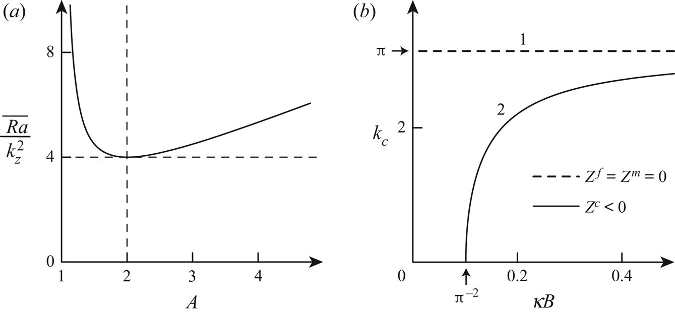
 \begin{equation} \frac{\overline{{\textit{Ra}}}}{k_z^2}=\frac{A^2}{A-1},\quad\mbox{where}\ A=\frac{\kappa B k^2+1}{\kappa B k_z^2}>1. \end{equation}
According to (6.9),  $A$ is an increasing function of
 $k^2$, whereas
 $\overline {{\textit {Ra}}}$ reaches a minimum of
 $4k_z^2=4{\rm \pi} ^2$ at
 $A=2$ (figure 3a), i.e. at
 \begin{equation} k_{xy}^2=k_z^2-\frac{1}{\kappa B}={\rm \pi}^2-\frac{1}{\kappa B}. \end{equation}
Equation (6.10) has a solution at  $\kappa B\geq {\rm \pi} ^{-2}$. Consequently, if
 $\kappa B\geq {\rm \pi} ^{-2}$, then (6.8) are satisfied simultaneously at
 $\overline {{\textit {Ra}}}=4{\rm \pi} ^2$, and if
 $\kappa B<{\rm \pi} ^{-2}$, then (6.8a) is satisfied before (6.8b) with increasing
 $\overline {{\textit {Ra}}}$. This yields
 \begin{equation} \overline{{\textit{Ra}}}_c=4{\rm \pi}^2,\quad k_{c}={\rm \pi}\quad\mbox{or}\quad k_{c}=\sqrt{{\rm \pi}^2-\frac{1}{\kappa B}}\quad\mbox{at}\ \kappa=\Lambda. \end{equation}
Figure 3(b) shows the critical wavenumbers (6.11) as solutions to (6.7). Straight line 1 and curve 2 are the solutions with  $Z^c>0$ and
 $Z^c<0$ to (6.8a) and (6.8b), respectively. The critical Rayleigh number is
 $4{\rm \pi} ^2$ for any such solution. As we have shown, only (6.8a) has a solution at
 $\kappa B<{\rm \pi} ^{-2}$. If
 $B\rightarrow 0$ or
 $B\rightarrow \infty$, then in accordance with (6.3) and (6.4),
 $k_c$ tends to
 ${\rm \pi}$ in both solutions.
(a) Value of  $\overline {{\textit {Ra}}}$ against
 $A$ as defined by (6.9). (b) The critical wavenumbers at
 $\kappa =\Lambda$.

In the case of  $k_c={\rm \pi}$ and
 $\overline {{\textit {Ra}}}={\textit {Ra}}^{\,f}={\textit {Ra}}^m=4{\rm \pi} ^2$, both
 $Z^{\,f}=0$ and
 $Z^m=0$, i.e. the conduction state in both media becomes unstable. Substituting
 $Z^{\,f}=0$,
 $Z^m=0$ and
 $\Omega =0$ into (4.11)–(4.13), we obtain
 \[ \delta\Theta^{\,f}=\delta\Theta^m,\quad \delta\Pi^{\,f}=\delta\Pi^m, \quad \delta q^{\,fm}=0. \]
Thus, the temperature and pressure amplitudes in the media are identical at  $k_c={\rm \pi}$,
 $\kappa =\Lambda$, any
 $B$ and
 $\overline {{\textit {Ra}}}=\overline {{\textit {Ra}}}_c$, meaning that the heat and mass transfer between
 $\Phi ^{\,j}$ is absent. Consequently, the flow pattern is identical to that in EPM.
6.4. Case $k_{xy}=0$ (the plane flow regime)

The dispersion equation (4.8) admits non-trivial solutions with zero horizontal wavenumbers, which do not exist in the case of homogeneous medium. To determine the Rayleigh numbers for which such solutions are possible, we substitute  $k_{xy}=0$ and
 $\Omega =0$ into (4.8), designate
 $\overline {{\textit {Ra}}}$ as
 $\overline {{\textit {Ra}}}_p$, and thereby obtain
 \begin{equation} \overline{{\textit{Ra}}}_p=\left(\kappa B k_z^2+1\right)\left(\Lambda B k_z^2+1\right)\frac{1-\Lambda}{\kappa(1-\kappa)B}. \end{equation}
If  $\overline {{\textit {Ra}}}>\overline {{\textit {Ra}}}_p$, then the problem admits the growing plane perturbations with
 $k_{xy}=0$. In what follows, we refer to such a flow pattern as the convection regime
 $P$. For
 $k_z={\rm \pi}$ (
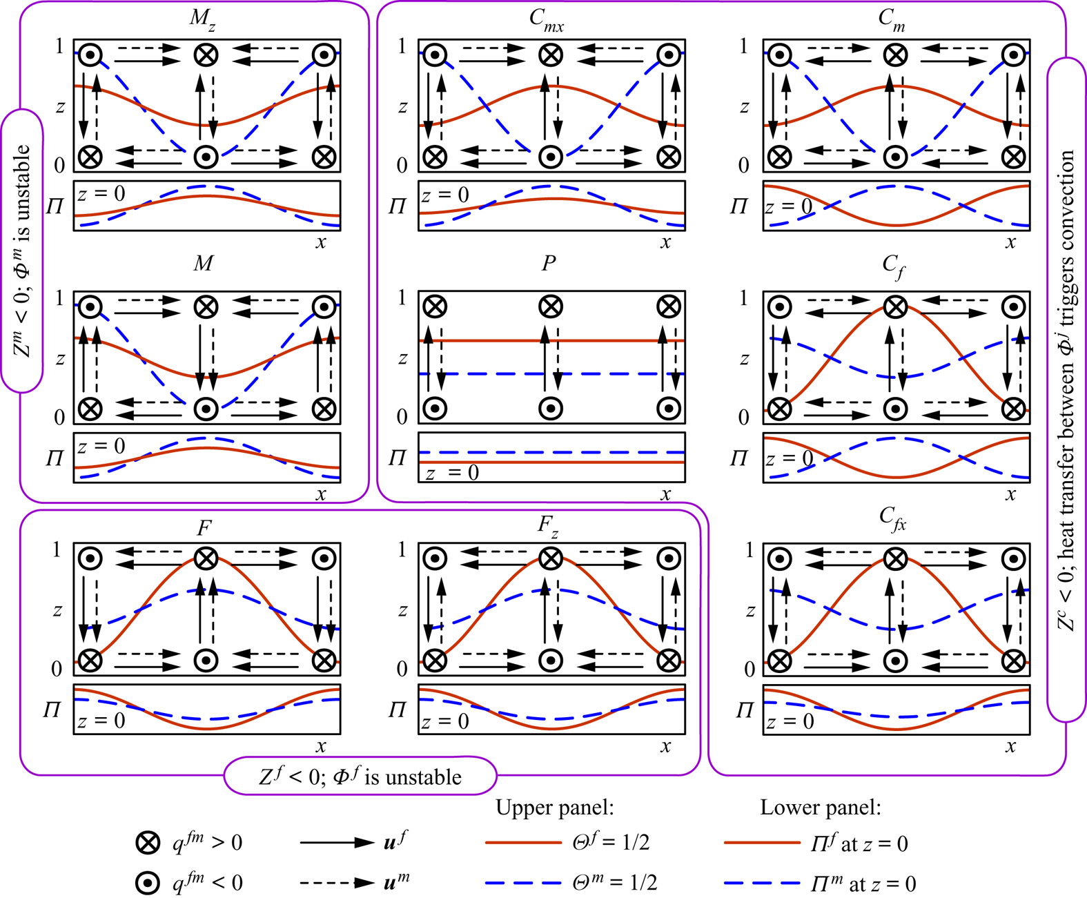
 $n=1$), it is schematically shown in figure 4 (in central panel
 $P$). The flow pattern consists of only the cross-medium convection cell (figure 1). For instance, the fluid can flow upward through
 $\Phi ^{\,f}$ (
 $u_z^{\,f}>0$), then into
 $\Phi ^m$ (
 $q^{\,fm}>0$) near the upper boundary of the layer (
 $z=1$), then downward through
 $\Phi ^m$ (
 $u_z^m<0$) and, finally, it flows back into
 $\Phi ^m$ (
 $q^{\,fm}<0$) near the lower boundary (
 $z=0$), thereby closing the cross-medium circulation. At the same time, according to (4.11), the inequality
 $\Theta ^{\,f}\geq \Theta ^m$ holds at any position vector
 $\boldsymbol {r}$. The circulation can occur in the opposite direction, and then,
 $\Theta ^{\,f}\leq \Theta ^m$.
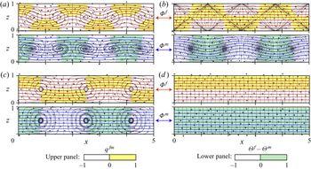
Possible convection regimes at  $\overline {{\textit {Ra}}}\rightarrow \overline {{\textit {Ra}}}_c+$. The isotherms
 $\Theta ^{\,j}=1/2$ and the direction of flow in convection cells are schematically shown in the upper panel for every regime. The pressure distributions,
 $\Pi ^{\,j}(x)$, at the lower boundary
 $z=0$ are shown in the lower panels.

At near-critical conditions, the plane flow regime appears if and only if  $\overline {{\textit {Ra}}}_c=\overline {{\textit {Ra}}}_p$, where
 $\overline {{\textit {Ra}}}_p$ is given by (6.12) with
 $k_z={\rm \pi}$. In general, with increasing
 $\overline {{\textit {Ra}}}$, the thermal stratification can first become unstable with respect to other perturbations with
 $k_{xy}>0$. Consequently, the inequality
 $\overline {{\textit {Ra}}}_c\leq \overline {{\textit {Ra}}}_p$ holds, and the opposite inequality
 $\overline {{\textit {Ra}}}>\overline {{\textit {Ra}}}_p$ is a sufficient condition for instability.
7. Parametric study
7.1. Flow regime classification
The numerical investigation of solutions to the dispersion equation (4.8) for  $\Omega =0$ and all possible
 $\kappa$,
 $\Lambda$ and
 $B$ shows that 9 flow regimes can arise at near-critical conditions. First, we discuss in general the convection patterns of these regimes, leaving for §§ 7.2 and 7.3 the description of parameters
 $\kappa$,
 $\Lambda$ and
 $B$ at which they occur.
The 9 regimes are further referred to as  $F$,
 $F_z$,
 $C_{fx}$,
 $C_f$,
 $C_m$,
 $C_{mx}$,
 $M_z$,
 $M$ and
 $P$ (figures4 and 5). The capital
 $F$ or
 $M$ refers to the fractures (
 $\Phi ^{\,f}$) or matrix (
 $\Phi ^m$) medium that is unstable at
 $\overline {{\textit {Ra}}}\rightarrow \overline {{\textit {Ra}}}_c$, respectively. The capital
 $C$ refers to the counter-rotating pattern that appears at
 $Z^c<0$ (see § 5). The capital
 $P$ corresponds to the plane regime considered in § 6.4. The regimes whose designation includes either the capital
 $F$ (or
 $M$) or the subscript
 $f$ (or
 $m$) are controlled mostly by the convective heat transfer through
 $\Phi ^{\,f}$ (or
 $\Phi ^m$). The regimes whose designation differs only by the presence of the subscript
 $x$ (or
 $z$) are the same except of the sign for
 $u^{\,j}_x$ (or
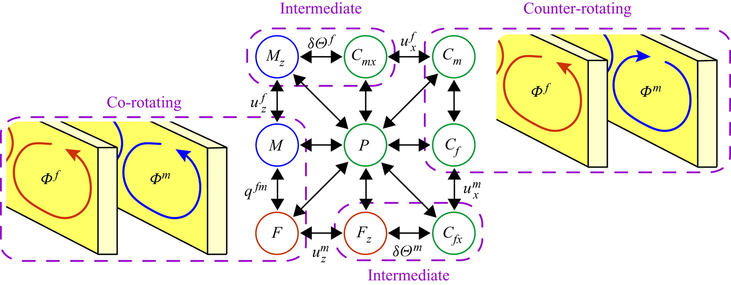
 $u^{\,j}_z$) in one of the media. For further discussion it is convenient to organize the regimes into 4 groups, namely, the co-rotating regimes
 $F$ and
 $M$; the counter-rotating regimes
 $C_f$ and
 $C_m$; the intermediate regimes
 $F_z$,
 $C_{fx}$,
 $C_{mx}$ and
 $M_z$ that appear in transition from co-rotating to counter-rotating patterns; and the regime
 $P$ (figure 5).
Possible transitions of the flow regimes. The dashed lines group the regimes in pairs of identical convection patterns in  $\Phi ^{\,j}$ but with different amplitudes
 $\delta \Pi ^{\,j}$ and
 $\delta \Theta ^{\,j}$ for
 $j=f,m$. The labels
 $u_x^{\,j}$,
 $u_z^{\,j}$,
 $q^{\,fm}$ and
 $\delta \Theta ^{\,j}$ designate transitions in which only the corresponding parameter changes sign.

The flow patterns and corresponding distributions of  $\Theta ^{\,j}$ and
 $\Pi ^{\,j}$ are schematically shown in figure 4. The diagram in figure 5 shows which flow pattern transitions are possible with continuous changes of the quantities
 $\kappa$,
 $\Lambda$ and
 $B$. For example, the regime
 $F$ can change only to
 $M$,
 $F_z$ or
 $P$. In other words, the region of parameters in the
 $\{\kappa ,\Lambda ,B\}$ space corresponding to the regime
 $F$ can have boundaries only with the regions corresponding to
 $M$,
 $F_z$ and
 $P$.
The regimes  $F$ and
 $F_z$ correspond to the inequality
 $Z^{\,f}<0$ at
 $\overline {{\textit {Ra}}}=\overline {{\textit {Ra}}}_c$, i.e. if the locus of solutions to (4.8) touches the conical surface
 $a_2=0$ at
 $Z^{\,f}<0$ (figure 2). Numerical analysis of the solutions to (4.8) indicates that these regimes can arise only if
 $\kappa \geq \Lambda$, i.e. if
 $\Phi ^{\,f}$ determines the flow pattern (
 ${\textit {Ra}}^{\,f}\geq 4{\rm \pi} ^2\geq {\textit {Ra}}^m$). This is in agreement with the theoretical analysis of the asymptotic case
 $B\rightarrow \infty$ discussed in § 6.2. In the regimes
 $F$ and
 $F_z$, the convection in DPM is triggered by the unstable conduction state in
 $\Phi ^{\,f}$ and the flow in
 $\Phi ^m$ appears only due to heat and mass transfer between the media. Therefore, and according to (4.11), in which
 $D^{\,j}=Z^{\,j}$ at
 $\Omega =0$, the absolute value of the temperature amplitude in
 $\Phi ^{\,f}$ is larger than that in
 $\Phi ^m$ (
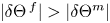 $|\delta \Theta ^{\,f}|>|\delta \Theta ^m|$).
Similarly, the regimes  $M$ and
 $M_z$ correspond to the inequality
 $Z^m<0$ at
 $\overline {{\textit {Ra}}}=\overline {{\textit {Ra}}}_c$, i.e. if the locus touches the conical surface
 $a_2=0$ at
 $Z^m<0$. As in the asymptotic case
 $B\rightarrow \infty$, these regimes can arise only if
 $\kappa \leq \Lambda$, i.e. if
 $\Phi ^m$ determines the flow pattern (
 ${\textit {Ra}}^m\geq 4{\rm \pi} ^2\geq {\textit {Ra}}^{\,f}$). The convection in these regimes is triggered by the unstable state in
 $\Phi ^m$, and the flow in
 $\Phi ^{\,f}$ appears only due to heat and mass transfer between the media. Therefore, and according to (4.11), the absolute value of the temperature amplitude in
 $\Phi ^m$ is larger than that in
 $\Phi ^{\,f}$ (
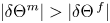 $|\delta \Theta ^m|>|\delta \Theta ^{\,f}|$).
According to (4.11), in which  $D^{\,j}=Z^{\,j}$ at
 $\Omega =0$, the temperature amplitudes
 $\delta \Theta ^{\,f}$ and
 $\delta \Theta ^m$ have identical signs for
 $F$,
 $F_z$,
 $M$ and
 $M_z$. Thus, higher (or lower) temperatures in
 $\Phi ^{\,f}$ correspond to higher (or lower) temperatures in
 $\Phi ^m$ in all 4 regimes.
The other 5 regimes –  $C_{fx}$,
 $C_f$,
 $C_m$,
 $C_{mx}$ and
 $P$ – correspond to the inequality
 $Z^c<0$ at
 $\overline {{\textit {Ra}}}=\overline {{\textit {Ra}}}_c$, i.e. if the locus of solutions to (4.8) touches the surface
 $a_2=0$ at
 $Z^c<0$. These regimes can arise at both
 $\kappa >\Lambda$ and
 $\kappa <\Lambda$. Therefore, the convection is not determined by only
 $\Phi ^{\,f}$ or
 $\Phi ^m$, which can result in more complicated flow patterns. For example, according to (4.11), the temperature amplitudes in
 $\Phi ^{\,f}$ and
 $\Phi ^m$ have opposite signs in these regimes (
 $\delta \Theta ^{\,f}\delta \Theta ^m<0$), i.e. higher (or lower) temperatures in
 $\Phi ^{\,f}$ correspond to lower (or higher) temperatures in
 $\Phi ^m$ (figure 4). Furthermore, a noteworthy observation is that the conduction states in
 $\Phi ^{\,f}$ and
 $\Phi ^m$ considered apart (isolated from each other) are stable because
 $Z^{\,f}>0$ and
 $Z^m>0$. The convection appears only if
 $\Phi ^{\,f}$ and
 $\Phi ^m$ are merged to form DPM. We can interpret this as that the heat transfer between the media triggers the onset of convection in regimes
 $C_{fx}$,
 $C_f$,
 $C_m$,
 $C_{mx}$ and
 $P$.
The co-rotating regimes  $F$ and
 $M$ are characterized with qualitatively similar flow fields, which are a simple generalization of the cellular convection cells in homogeneous porous medium, i.e. EPM (Nield & Bejan Reference Nield and Bejan2017). Horizontal and vertical components of the fluid velocities in
 $\Phi ^{\,f}$ and
 $\Phi ^m$ for any position vector
 $\boldsymbol {r}$ have equal signs corresponding to co-rotating cells in both media (figure 4). The regimes
 $F$ and
 $M$ differ only in the direction of fluid flow between
 $\Phi ^{\,j}$ and the amplitudes
 $\delta \Pi ^{\,j}$ and
 $\delta \Theta ^{\,j}$. In the regime
 $F$ (or
 $M$), the convection in
 $\Phi ^{\,f}$ (or
 $\Phi ^m$) dominates over that in
 $\Phi ^m$ (or
 $\Phi ^{\,f}$), leading to larger absolute values of
 $\delta \Theta ^{\,f}$ and
 $\delta \Pi ^{\,f}$ (or
 $\delta \Theta ^m$ and
 $\delta \Pi ^m$). At the same time, in the regime
 $F$, the medium
 $\Phi ^{\,f}$ withdraws fluid from
 $\Phi ^m$ at the bottom of ascending currents due to lower pressure
 $\Pi ^{\,f}$ (
 $q^{\,fm}<0$ at
 $z=0$) and returns it back to
 $\Phi ^m$ at the top of the currents (
 $q^{\,fm}>0$ at
 $z=1$).
Let us consider how the flow pattern changes with varying  $\kappa$,
 $\Lambda$ and
 $B$ in the following sequence of transitions (corresponding to the counter-clockwise movement around
 $P$ in figures 4 and 5):
 \begin{equation} F\rightarrow F_z\rightarrow C_{fx}\rightarrow C_f. \end{equation}
The transition from the co-rotating regime  $F$ to the intermediate regime
 $F_z$ is characterized by increasing intensity of the fluid withdrawal at the bottom of the ascending current. When entering the regime
 $F_z$, the withdrawal becomes so intense that it reverts the vertical direction of flow in
 $\Phi ^m$. Now, the fluid in
 $\Phi ^m$ converges to the bottom of ascending currents in
 $\Phi ^{\,f}$, which can be considered as sink zones for the medium
 $\Phi ^m$. Similarly, the top of ascending currents in
 $\Phi ^{\,f}$ are the source zones for
 $\Phi ^m$ from which the flow diverges through
 $\Phi ^m$. Thus, the transition from
 $F$ to
 $F_z$ breaks down convection cells in
 $\Phi ^m$ and leads to the appearance of new cross-media cells as in the
 $P$ regime. At every
 $x,y=\mbox {const}$ in the cross-media cells, the fluid ascends through
 $\Phi ^{\,f}$ (or
 $\Phi ^m$) and flows to the adjacent medium
 $\Phi ^m$ (or
 $\Phi ^{\,f}$) at the top of ascending currents, then it flows down in the descending currents through the medium
 $\Phi ^m$ (or
 $\Phi ^{\,f}$), and ultimately flows back to
 $\Phi ^{\,f}$ (or
 $\Phi ^m$) at
 $z=0$, closing the circulation (figure 1).
The intermediate regimes  $F_z$ and
 $C_{fx}$ have identical convection patterns and different temperature distributions in
 $\Phi ^m$. Transition from
 $F_z$ to
 $C_{fx}$ is characterized by increasing influence of convective heat transfer through
 $\Phi ^m$ as compared to that between
 $\Phi ^{\,j}$. Consequently, the temperature amplitude
 $\delta \Theta ^m$ changes its sign when entering
 $C_{fx}$, and the inequality
 $\delta \Theta ^{\,f}\delta \Theta ^m<0$ holds in the regime
 $C_{fx}$. Now, the descending (or ascending) currents in
 $\Phi ^m$ move the isotherms
 $\Theta ^m=\mbox {const}$ downward (or upward).
The transition from  $C_{fx}$ to
 $C_f$ is characterized by a further increasing influence of the reversed flow direction in
 $\Phi ^m$. At the transition, the horizontal velocity in
 $\Phi ^m$ changes its sign, and new cellular convection with opposite direction of circulation forms in
 $\Phi ^m$. Thus, the flow pattern in the regime
 $C_f$ consists of counter-rotating cells in the media
 $\Phi ^{\,f}$ and
 $\Phi ^m$. At the same time, the cross-medium convection cells also exist (figure 4).
The flow fields in regimes  $C_f$ and
 $C_m$ are qualitatively similar, with different amplitudes of pressure and temperature. The temperature amplitudes
 $\delta \Theta ^{\,f}$ and
 $\delta \Theta ^m$ have opposite signs (
 $\delta \Theta ^{\,f}\delta \Theta ^m<0$) reflecting the counter-rotating behaviour of convection. Here, the dominant feature is the convective heat transfer through the media that moves the isotherms in
 $\Phi ^{\,f}$ and
 $\Phi ^m$ in opposite directions. The heat transfer between
 $\Phi ^{\,j}$ does not significantly affect
 $\delta \Theta ^{\,j}$ because it is secondary. By definition, the boundary between
 $C_f$ and
 $C_m$ corresponds to equal absolute values of
 $\delta \Theta ^{\,f}$ and
 $\delta \Theta ^m$. The inequalities
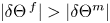 $|\delta \Theta ^{\,f}|>|\delta \Theta ^m|$ and
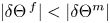 $|\delta \Theta ^{\,f}|<|\delta \Theta ^m|$ hold in regimes
 $C_f$ and
 $C_m$, respectively. Transition from
 $C_f$ to
 $C_m$ is characterized by increasing influence of convective heat transfer through
 $\Phi ^m$ as compared to that through
 $\Phi ^{\,f}$. From now on, if we consider the regimes
 $C_m$,
 $C_{mx}$,
 $M_z$ and
 $M$ (figure 4), the convection in
 $\Phi ^m$ determines the flow pattern.
The transition sequence
 \[ M\rightarrow M_z\rightarrow C_{mx}\rightarrow C_m \]
is characterized by the processes in the media  $\Phi ^m$ and
 $\Phi ^{\,f}$, which mirror the processes in the media
 $\Phi ^{\,f}$ and
 $\Phi ^m$ in the sequence (7.1) described in detail above. In short, when entering
 $M_z$ from
 $M$, the vertical velocity
 $u_z^{\,f}$ in
 $\Phi ^{\,f}$ changes sign. When entering
 $C_{mx}$, the temperature amplitude
 $\delta \Theta ^{\,f}$ changes sign. When entering
 $C_m$, the horizontal velocity
 $u^{\,f}_x$ in
 $\Phi ^{\,f}$ reverts direction and cellular convection in
 $\Phi ^{\,f}$ with an opposite direction of circulation forms (figure 5).
7.2. Solution map at $B=\mbox {const}$

Now, we constrain the regions of the  $\{\kappa ,\Lambda ,B\}$ space corresponding to each convection regime. First, we consider the numerical solutions to the dispersion equation (4.8) for fixed
 $B$ and different
 $\kappa$ and
 $\Lambda$ (figure 6). The numerical solution indicates that only the transitions shown in figure 5 are possible. The straight line
 $\kappa =\Lambda$ for any
 $B$ is the boundary between a pair of flow regimes. In agreement with the asymptotic case
 $B\rightarrow \infty$ (see § 6.2), regimes
 $F$ and
 $F_z$ can arise only at
 $\kappa \geq \Lambda$, i.e. below the straight line
 $\kappa =\Lambda$, whereas
 $M$ and
 $M_z$ can arise only at
 $\kappa \leq \Lambda$, i.e. above the straight line
 $\kappa =\Lambda$. The regimes
 $C_{fx}$,
 $C_f$,
 $C_m$,
 $C_{mx}$ and
 $P$ can arise near the straight line
 $\kappa =\Lambda$ and in a wider region at
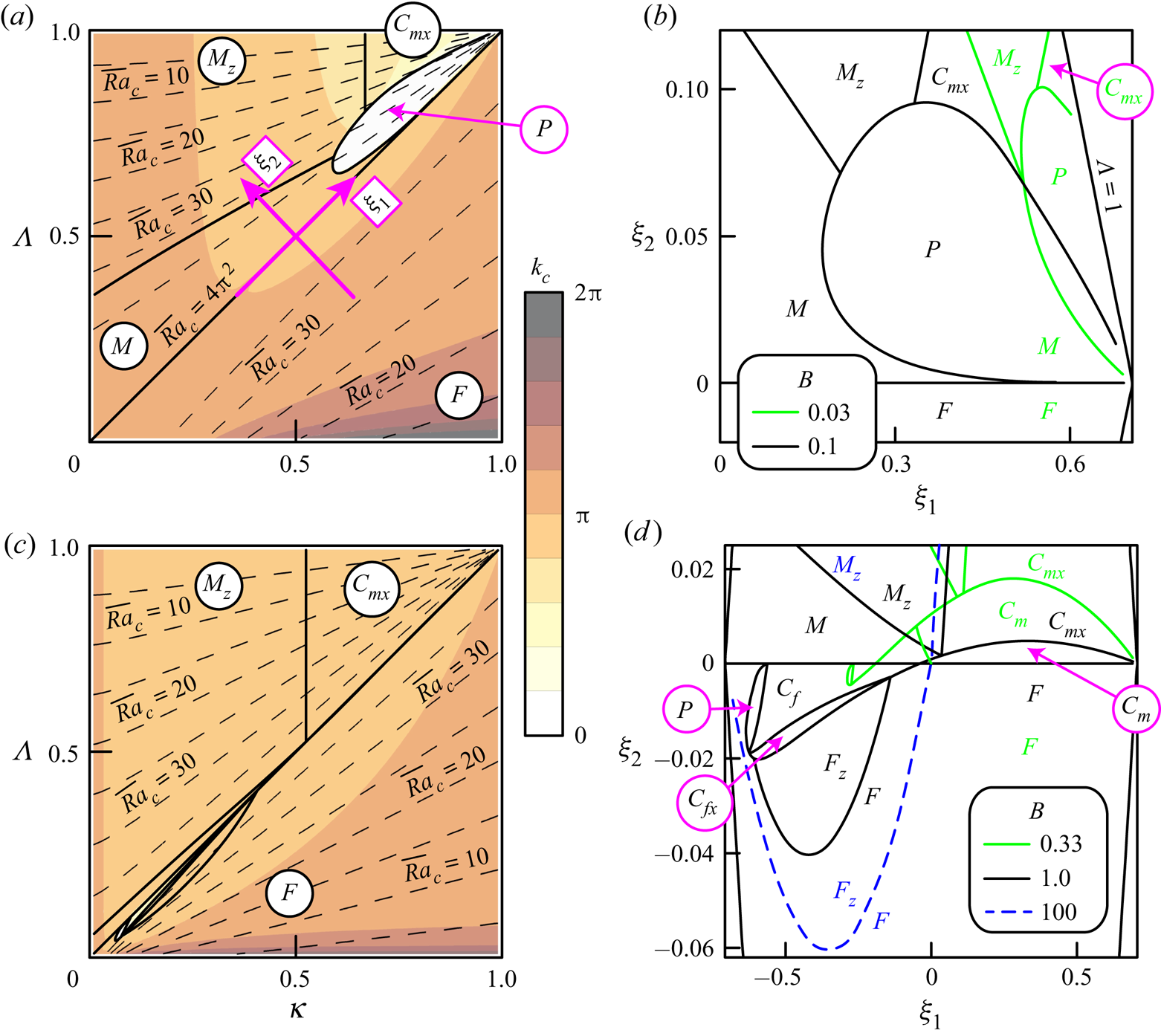
 $\Lambda >\kappa >1/2$. To make the boundaries of the flow regimes near the straight line
 $\kappa =\Lambda$ more distinct, we show the solution map in both the
 $\{\kappa ,\Lambda \}$ plane (figure 6a,c) and the
 $\{\xi _1,\xi _2\}$ plane (figure 6b,d), where
 \[ \xi_1=\frac{1}{\sqrt{2}}\left(\kappa+\Lambda-1\right),\quad \xi_2=\frac{1}{\sqrt{2}}\left(\Lambda-\kappa\right). \]
Thus, the origin of the  $\{\xi _1,\xi _2\}$ plane is the point
 $\kappa =\Lambda =1/2$ in the
 $\{\kappa ,\Lambda \}$ plane (figure 6a).
Solutions to the dispersion equation for (a,b)  $B=0.1$ and (c,d)
 $B=1$. The solution maps for other values of
 $B$ are also shown in the panels (b,d). The solid lines separate different flow regimes. The dashed lines in (a,c) are the contour lines of
 $\overline {{\textit {Ra}}}_c$ with step 5.

As discussed in § 6.1, if  $B\rightarrow 0$ (i.e. if
 $\Phi ^{\,j}$ are under local equilibrium), then the solution map contains only two regions
 $\kappa >\Lambda$ and
 $\kappa <\Lambda$ corresponding to the regimes
 $F$ and
 $M$, respectively. When
 $B$ increases from 0 (i.e. the degree of local non-equilibrium increases), the regions
 $M_z$,
 $P$ and
 $C_{mx}$ appear at
 $\kappa \rightarrow 1$,
 $\Lambda \rightarrow 1$ and
 $\kappa <\Lambda$ (figure 6b,
 $B=0.03$). When
 $B$ increases to 0.1, the regions
 $M_z$,
 $C_{mx}$ and
 $P$ expand downward and leftward along the straight line
 $\kappa =\Lambda$ (
 $\xi _2=0$), and the area of the region
 $P$ reaches a maximum at
 $B\approx 0.1$ (figure 6b).
When  $B$ increases from 0.1 to 1, the region
 $Z^c<0$, corresponding to the counter-rotating and plane regimes, expands across the straight line
 $\kappa =\Lambda$ into the region
 $\kappa >\Lambda$ and
 $\kappa <1/2$ (figure 6c,d). In addition, the region
 $C_m$ appears inside the envelope curve bounding the region
 $P$. Then, the boundary between
 $P$ and
 $C_m$ moves downward and leftward (along the straight line
 $\kappa =\Lambda$ corresponding to equal distributions of
 $\overline {K}$ and
 $\overline {\lambda }$ between
 $\Phi ^{\,j}$), which results in the disappearance of the region
 $P$ at
 $\kappa <\Lambda$. At
 $\kappa >\Lambda$, the regions
 $F_z$,
 $C_{fx}$ and
 $C_{f}$ appear, with the region
 $F_z$ growing downward from
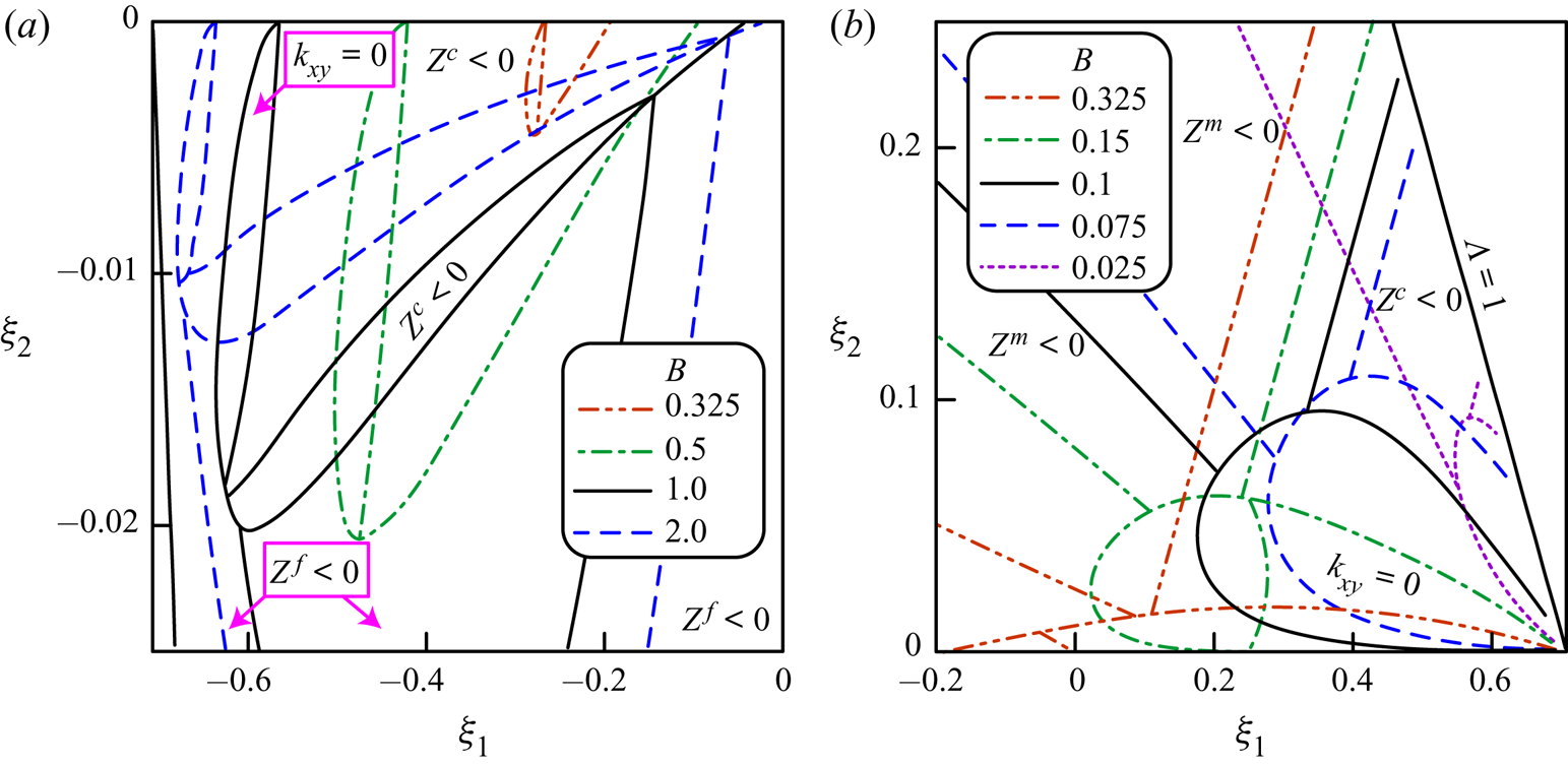
 $C_{fx}$. A more detailed evolution of the solution map near the straight line
 $\kappa =\Lambda$ when
 $B$ increases from 0.025 to 2.0 is shown in figure 7.
Boundaries of the convection regimes in the  $\{\xi _1,\xi _2\}$ plane. See figure 6 for reference between the solution map and the convection regimes. The conditions
 $Z^{\,f}<0$,
 $Z^m<0$,
 $Z^c<0$ and
 $k_{xy}=0$ are satisfied in the corresponding regions bounded by the solid lines.

When  $B$ increases from 1 to 100, all regions except
 $F$,
 $M_z$ and
 $C_{mx}$ shrink to the straight line
 $\kappa =\Lambda$. The solution map for
 $B>100$ is indistinguishable from the map at
 $B=100$ shown in figure 6(d). According to (4.11) and (4.12), the amplitudes
 $\delta \Theta ^{\,f}$ and
 $\delta \Pi ^{\,f}$ tend to zero in the region
 $\kappa <\Lambda$ at
 $\Omega =0$ and
 $B\rightarrow \infty$ (
 $Z^m=0$ or
 $Z^c=0$), and the amplitudes
 $\delta \Theta ^m$ and
 $\delta \Pi ^m$ tend to zero in the region
 $\kappa >\Lambda$ (
 $Z^{\,f}=0$ or
 $Z^c=0$). Thus, the convection only in
 $\Phi ^m$ (or
 $\Phi ^{\,f}$) develops if
 $\kappa <\Lambda$ (or
 $\kappa >\Lambda$) and
 $B\rightarrow \infty$. This observation agrees with the analytical investigation of the case
 $B\rightarrow \infty$ carried out in § 6.2.
As shown in figure 6(a), there is a sharp transition to the regime  $P$ from any other regime. When entering the regime
 $P$, the wavenumber
 $k_{c}$ sharply decreases to 0 and the solution bifurcates to
 $P$. At the same time,
 $\overline {{\textit {Ra}}}_c$ changes continuously. Other transitions, which are not into
 $P$ or across the straight line
 $\kappa =\Lambda$ (see (6.11)), are continuous rather than sharp bifurcations.
In general, all except two boundaries between the convection regimes at  $B=\mbox {const}$ are curved lines, which cannot be described with a finite readable relationship. The first exception is the straight line
 $\kappa =\Lambda$. Let us prove that the boundary between
 $M_z$ and
 $C_{mx}$, characterized with the condition
 $\delta \Theta ^{\,f}=0$ (figure 5), is the straight line
 $\kappa =\mbox {const}$, i.e. the second exception. The parameters of any point belonging to this line satisfy the following system of equations:
 \begin{equation} Z^m=0,\quad Z^c=0,\end{equation}
 \begin{equation} \frac{\mathrm{d}}{\mathrm{d}k^2}\left(Z^{\,f}Z^m+Z^{\,f}Z^c+Z^mZ^c\right)=0.\end{equation}
Equations (7.2a) indicate that the line is the boundary between the regimes  $M_z$ (
 $Z^m<0$ and
 $Z^c>0$) and
 $C_{mx}$ (
 $Z^m>0$ and
 $Z^c<0$). The dispersion equation (4.8) is satisfied by (7.2a). Equation (7.2b) indicates that the locus of solutions to (4.8) touches the surface
 $a_2=0$ (figure 2). Here,
 $k^2$ is considered as the locus parameter. With account for (7.2a), (7.2b) simplifies to
 \begin{equation} \frac{\mathrm{d}}{\mathrm{d}k^2}\left(Z^m+Z^c\right)=0. \end{equation}
Differentiating (4.9b) and (4.17), we obtain
 \begin{equation} \frac{\mathrm{d} Z^m}{\mathrm{d}k^2}=\frac{1-\Lambda}{\overline{{\textit{Ra}}}}-(1-\kappa)\frac{k_z^2}{k^2},\quad \frac{\mathrm{d} Z^c}{\mathrm{d}k^2}=(1-\kappa)\kappa\frac{2k^2\kappa B+1}{(k^2\kappa B+1)^2}\frac{k_z^2}{k^4}. \end{equation}
Substituting (4.9b), (4.17) and (7.4) into (7.2a) and (7.3), we derive the system of three algebraic equations. After excluding  $\overline {{\textit {Ra}}}$ and
 $k_{xy}^2$ from that system and carrying out identity transformations, we obtain
 \begin{equation} \kappa=\frac{Bk_z^2+1}{2Bk_z^2+1}. \end{equation}
For  $B=\mbox {const}$, (7.5) gives a vertical straight line in the plane
 $\{\kappa ,\Lambda \}$ between the regimes
 $M_z$ and
 $C_{mx}$. According to (7.5), if
 $B=0$, then
 $\kappa =1$, and with increasing
 $B$, the boundary between
 $M_z$ and
 $C_{mx}$ moves leftward in the plane
 $\{\kappa ,\Lambda \}$ approaching the straight line
 $\kappa =1/2$ in the limit
 $B\rightarrow \infty$.
7.3. Solutions at $\kappa =\mbox {const}$ or $\Lambda =\mbox {const}$


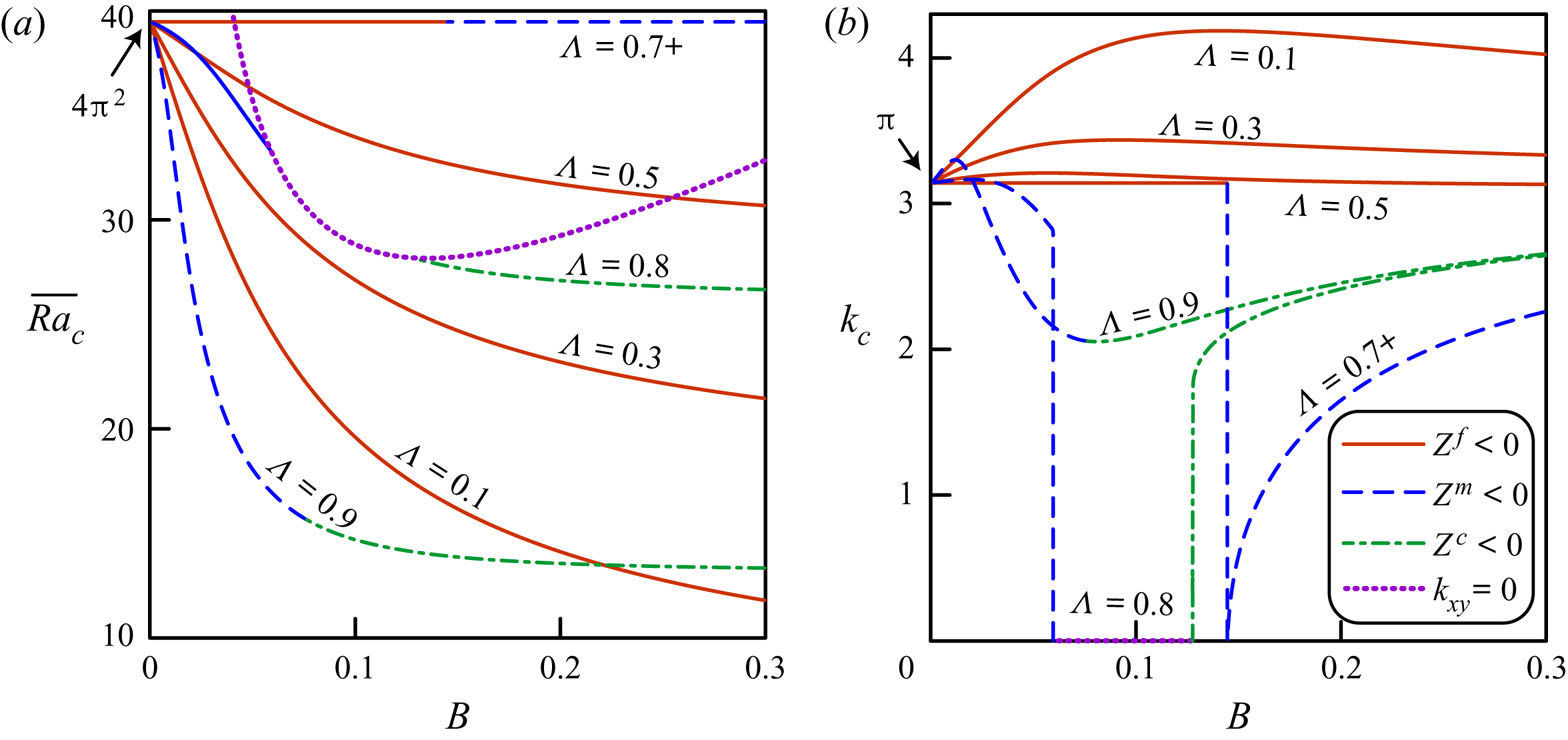
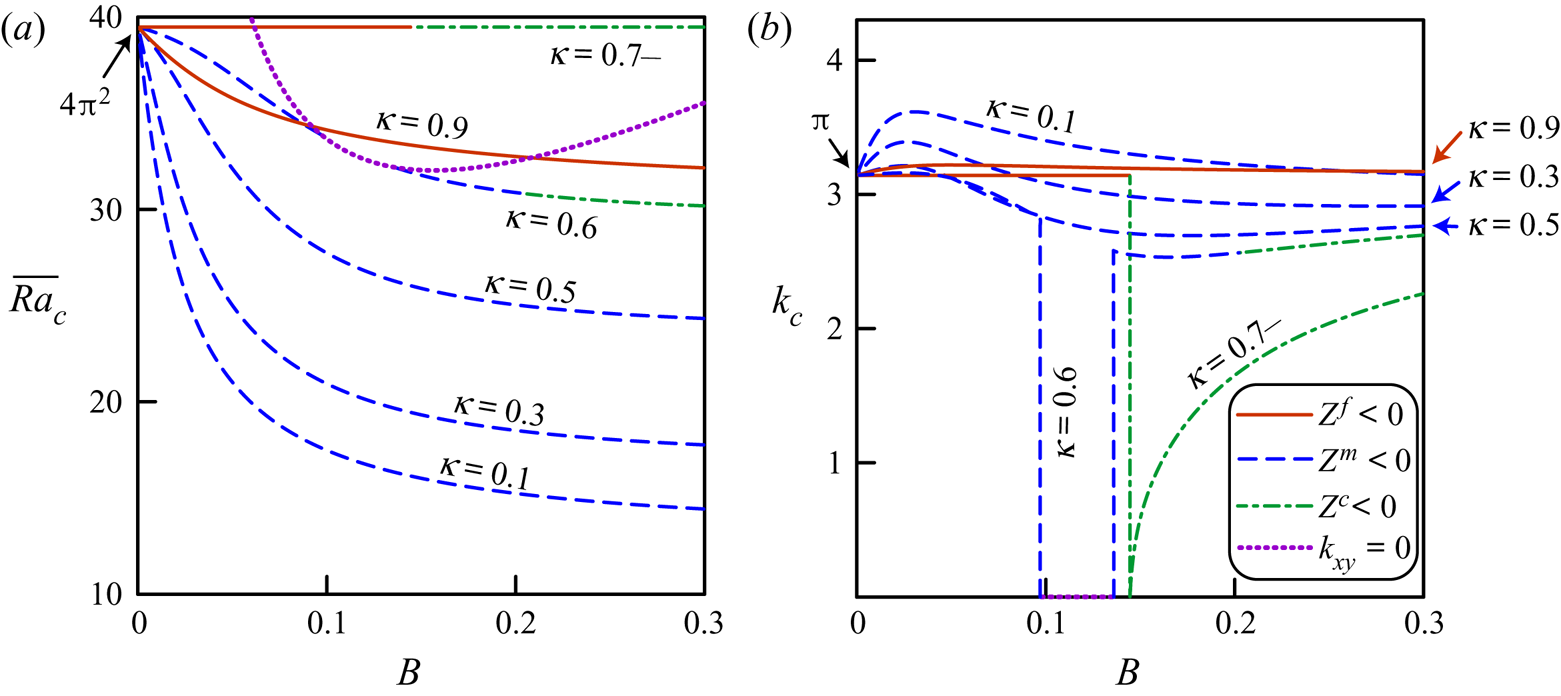
The solutions to (4.8) for fixed  $\kappa =0.7$ and
 $\Lambda =0.7$ are shown in figures 8 and 9, respectively. The style of the contour lines shows the type of solution, either
 $Z^{\,f}<0$ (regimes
 $F$ and
 $F_z$) or
 $Z^m<0$ (regimes
 $M$ and
 $M_z$), or
 $Z^c<0$ (regimes
 $C_{fx}$,
 $C_{f}$,
 $C_m$ and
 $C_{mx}$), or
 $k_{xy}=0$ (regime
 $P$). If
 $B\rightarrow 0$, then, in agreement with (6.5),
 $\overline {{\textit {Ra}}}_c\rightarrow 4{\rm \pi} ^2$ and
 $k_c\rightarrow {\rm \pi}$. For any
 $B$, the critical Rayleigh number is not higher than
 $4{\rm \pi} ^2$, and thus,
 $\overline {{\textit {Ra}}}_c$ for DPM does not exceed
 $\overline {{\textit {Ra}}}_c$ for EPM (figures 8a and 9a). This result demonstrates that DPM differs from BDPM, in which LTNE can increase the value of
 $\overline {{\textit {Ra}}}_c$ (Nield & Kuznetsov Reference Nield and Kuznetsov2006). The critical wavenumber
 $k_c$ can be either higher or lower than
 ${\rm \pi}$. When entering the regime
 $P$,
 $k_c$ abruptly decreases to 0 and the solution bifurcates into the plane flow pattern (figures 8b and 9b).
Solutions to the dispersion equation at  $\kappa =0.7$ against variable
 $B$. The dotted curve is given by (6.12) at
 $\Lambda =0.8$.

Solutions to the dispersion equation at  $\Lambda =0.7$ against variable
 $B$. The dotted curve is given by (6.12) at
 $\kappa =0.6$.

The labels  $\Lambda =0.7+$ and
 $\kappa =0.7-$ mean that
 $\Lambda$ and
 $\kappa$ are slightly less than or higher than 0.7, respectively. The contour lines
 $\Lambda =0.7+$ at
 $\kappa B\geq {\rm \pi} ^{-2}$ and
 $\kappa =0.7-$ at
 $\Lambda B\geq {\rm \pi} ^{-2}$ correspond to the second solution for
 $k_c$ in (6.11). As shown in figure 3(b), the contour lines
 $\Lambda =0.7-$ and
 $\kappa =0.7+$ would be straight lines
 $k_c={\rm \pi}$ corresponding to the first solution for
 $k_c$ in (6.11).
The numerical solutions to (4.8) indicate that the conclusions of this section are valid for any constant value of  $\kappa$ or
 $\Lambda$ other than 0.7.
8. Numerical experiments
To support the analytical findings of the previous sections, we conduct numerical modelling of convection in DPM using the reservoir simulator MUFITS (Afanasyev Reference Afanasyev2017). The simulations are performed using the dual-porosity dual-permeability concept with (2.6) assumed to hold. The system of governing equations used in the modelling, which in the Oberbeck–Boussinesq approximation reduces to (2.1)–(2.4), can be derived from Pruess (Reference Pruess1983), Pruess & Narasimhan (Reference Pruess and Narasimhan1985), Dietrich et al. (Reference Dietrich, Helmig, Sauter, Teutsch, Hötzl and Köngeter2005) and Berre, Doster & Keilegavlen (Reference Berre, Doster and Keilegavlen2019). The inequality  $\alpha \ll 1$ holds; thus, the Oberbeck–Boussinesq approximation is applicable with a sufficient degree of accuracy.
In dimensionless units, we consider the two-dimensional domain of finite width 5,  $x\in [0,5]$, for which the boundaries
 $x=0$ and
 $x=5$ are assumed to be impermeable and adiabatic (figure 10). The parameters of 4 considered simulation scenarios are summarized in table 1, whereas other dimensionless quantities are
 $S^{\,f}=1.5$,
 $S^m=3.0$,
 $\alpha =3.6\cdot 10^{-3}$ and
 $\Upsilon =2.1\cdot 10^{-5}$. The
 $\overline {{\textit {Ra}}}$ number is chosen to be less than 10 % higher than
 $\overline {\textit{Ra} }_c$ (
 $\overline {\textit{Ra} }\leq 1.1\overline {{\textit {Ra}}}_c$). Consequently, the layer is at slightly super-critical conditions, for which the theoretical study is presented. Details of the numerical algorithm and the simulation results as well as animated figures showing the convection development are included in the supplementary material available at https://doi.org/10.1017/jfm.2020.462.
(a–d) Simulated convection patterns for the regimes  $F$,
 $M_z$,
 $C_f$ and
 $P$, respectively. The bold curves show isotherms
 $\Theta ^{\,j}=i/10$,
 $i=1\ldots 9$, the thin curves are the streamlines and the arrows indicate the direction of the fluid flow in
 $\Phi ^{\,f}$ (upper panels) and
 $\Phi ^m$ (lower panels), respectively.

Parameters of the considered simulation scenarios.

The flow patterns evolving at  $t>100$ from the quiescent stratified fluid at
 $t=0$ are shown in figure 10. The simulations are in agreement with the analytical study that predicts the appearance of the
 $F$,
 $M_z$,
 $C_f$ and
 $P$ regimes, respectively. Indeed, the simulated patterns replicate those schematically shown in figure 4. Also, the horizontal dimensions of the convection cells are in line with the critical wavelength
 $k_c$. According to (4.6) and (4.14), the regions where the heat is transferred from
 $\Phi ^{\,f}$ to
 $\Phi ^m$ by means of convection (
 $q^{\,fm}>0$) and thermal conduction (
 $\Theta ^{\,f}-\Theta ^m>0$) do not coincide. An interesting feature is that the streamlines in the convection cells can be spiral curves converging to the cell centres rather than closed curves. This is explained by the mass transfer between
 $\Phi ^{\,j}$ in the weakly nonlinear regimes at
 $\overline {{\textit {Ra}}}_c<\overline {{\textit {Ra}}}\leq 1.1\overline {Ra}_c$.
9. Conclusions
The study shows that Darcy–Bénard convection in a horizontal layer of DPM with isothermal impermeable boundaries can occur by the onset of nine different flow regimes. Most of these regimes are driven by the convective heat transport in both media  $\Phi ^{\,j}$. The regimes include the flow patterns with the co-rotating or counter-rotating convection cells in the adjacent media, as well as the plane flow field with only the cross-medium circulation. We show that the critical Rayleigh number depends on three parameters, namely, the ratios of permeability and heat conductivity in the media and the dimensionless number characterizing the intensity of heat and mass transfer between
 $\Phi ^{\,j}$. We provide complete classification of the flow regimes and plot them in the solution map.
In the asymptotic cases of local thermal equilibrium ( $B\rightarrow 0$) or the absence of heat and mass exchange between
 $\Phi ^{\,j}$ (
 $B\rightarrow \infty$), only the co-rotating flow regimes, which are a simple generalization of the cellular flow pattern in the HRL problem for homogeneous medium, can arise. The most unexpected counter-rotating and plane convection patterns arise when the heat transfer between
 $\Phi ^{\,j}$ is comparable to that through the media (i.e. at
 $0.01\leq B\leq 10$). However, these regimes occur only if the ratios of permeability and heat conductivity in the media are close to each other (
 $\kappa \approx \Lambda$). For the considered boundary conditions at
 $z=0$ and
 $z=1$, the co-rotating convection occurs within a much wider range of parameters.
A noteworthy conclusion for geophysical applications is that the critical Rayleigh number for the fractured-porous medium is not higher than that for the equivalent homogeneous medium. Therefore, the onset of convection in fractured reservoirs occurs for vertical gradients of temperature, which are not higher than that in the homogeneous reservoirs for any parameters of the layer. For a fixed bulk permeability, the fractures reduce the critical Rayleigh number, i.e. the thermal stratification is less stable in a fractured-porous medium than that in the equivalent homogeneous medium. This result agrees with the study by Nield & Simmons (Reference Nield and Simmons2007), who concluded that heterogeneity of a porous medium leads to reduction of the critical Rayleigh number. We extend it by concluding that the thermal stratification in a fractured-porous medium is most stable if the bulk permeability and the bulk heat conductivity are distributed in equal proportions between fractures and matrix.
The present study can be applied for predicting convection patterns for a variety of geophysical applications, in addition to the numerical studies by Simmons et al. (Reference Simmons, Sharp and Nield2008), Vujević et al. (Reference Vujević, Graf, Simmons and Werner2014) and others, who also report counter-rotating convection cells, although in a slightly different context. The work still to be done is the study extension to the cases of other boundary conditions at  $z=0$ and
 $z=1$. In the geophysical context, the case of open boundary
 $z=1$ would be most significant because it corresponds to a hydrothermal system interacting through
 $z=1$ with shallow meteoric water. Even the considered case of impermeable isothermal boundaries can further be extended by accounting for anisotropic permeability in
 $\Phi ^{\,j}$ and
 $B_1\ne B_2$. Preliminary study of the
 $B_1\ne B_2$ situation shows that the region of counter-rotating and plane regimes at
 $B_2=\text {const}$ expands significantly with decreasing ratio
 $B_1/B_2$. Therefore, the likelihood of such regimes increases if the rate of approaching the local equilibrium for temperatures is lower than that for pressures, but this is a subject of further research.
Acknowledgments
Funding for this work was provided by the RF President's Council on Grants (MD-3567.2018.1).
Declaration of interests
The author reports no conflict of interest.
Supplementary material and movies
Supplementary material and movies are available at https://doi.org/10.1017/jfm.2020.462.