1. Introduction
Since Tanner & Blows (Reference Tanner and Blows1976) and Tanner & Kulkarny (Reference Tanner and Kulkarny1976) introduced the oil-film and oil-drop technique to measure wall shear stress of air flows, it has slowly gained ground relative to other methods, as documented by Janke (Reference Janke1993), Fernholz et al. (Reference Fernholz, Janke, Schober, Wagner and Warnack1996), Brown & Naughton (Reference Brown and Naughton1999), Rüedi et al. (Reference Rüedi, Nagib, Österlund and Monkewitz2003) and Vinuesa et al. (Reference Vinuesa, Bartrons, Chiu, Dressler, Rüedi, Suzuki and Nagib2014), for instance. The oil-film method, where a large wall area is covered with an oil film, is used rather rarely but the oil-drop method, where small individual oil drops are deposited on the wall, has over the last decade become the method of choice for the independent determination of wall shear stress. As such it is a cornerstone of recent experimental turbulent-boundary-layer research by Österlund (Reference Österlund1999), Nagib, Chauhan & Monkewitz (Reference Nagib, Chauhan and Monkewitz2007), Nagib & Chauhan (Reference Nagib and Chauhan2008) and Chauhan, Monkewitz & Nagib (Reference Chauhan, Monkewitz and Nagib2009), for instance, and its accuracy is a central issue in the ongoing debate on turbulent-boundary-layer scalings (see for instance Marusic et al. Reference Marusic, McKeon, Monkewitz, Nagib, Smits and Sreenivasan2010; Alfredsson et al. Reference Alfredsson, Imayama, Lingwood, Örlü and Segalini2013) and in the recent international comparison of different turbulent-boundary-layer facilities (see Nagib et al. Reference Nagib, Smits, Marusic and Alfredsson2009; Rüedi et al. Reference Rüedi, Duncan, Imayama and Chauhan2009; Bailey et al. Reference Bailey, Hultmark, Monty, Alfredsson, Chong, Duncan, Fransson, Hutchins, Marusic, McKeon, Nagib, Örlü, Segalini, Smits and Vinuesa2013).
Until now, the extraction of wall shear stress from the evolution of oil drops has been based on the basic similarity solution (see Tanner & Blows Reference Tanner and Blows1976) for the thickness of a wedge-shaped two-dimensional oil film entrained by a zero-pressure-gradient turbulent boundary layer, henceforth abbreviated ‘ZPG TBL’:
 $$\begin{eqnarray}h^{\ast }(x^{\ast },t^{\ast })=\frac{{\it\mu}_{oil}^{\ast }x^{\ast }}{{\it\tau}_{w}^{\ast }t^{\ast }},\end{eqnarray}$$
where
 ${\it\mu}_{oil}^{\ast }$
is the dynamic viscosity of oil,
 ${\it\tau}_{w}^{\ast }$
the wall shear stress of the air boundary layer entraining the oil and
 $\text{}^{\ast }$
superscripts denote dimensional quantities throughout the paper. Hence, with
 ${\it\mu}_{oil}^{\ast }$
known,
 ${\it\tau}_{w}^{\ast }$
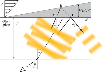
is obtained directly from the time evolution of the oil-wedge angle. In practice the latter is determined with a Fizeau interferometer. Its typical set-up for the oil-drop technique, which has virtually become the standard, is shown schematically in figure 1.
Typical set-up with an oil drop of thickness
 $h^{\ast }(x^{\ast },t^{\ast })$
(shaded) on an optical window of thickness
 $d^{\ast }$
. The sketch represents the symmetry plane of the oil drop and includes the definition of coordinates and the optical path of the Fizeau interferometer (note that the slope of the oil–air interface is grossly exaggerated to make visible the difference between the wavevector angles
 ${\it\theta}_{i}$
and
 ${\it\theta}_{o}$
). – ⋅ – ⋅ –, Direction from which interference fringes are seen (
 ${\it\theta}=({\it\theta}_{i}+{\it\theta}_{o})/2$
within the glass window). Specifics of our set-up are given in § 2.8.

The set-up includes an optical window of thickness
 $d^{\ast }$
mounted in a flush-wall plug on which the oil drop is deposited and through which it is observed from the outside of the flow facility. Also shown in the figure is the optical path of the Fizeau interferometer used to measure the oil-film thickness
 $h^{\ast }(x^{\ast },t^{\ast })$
. In an actual set-up, the observation angle
 ${\it\varphi}$
is chosen first (note that this angle varies slightly over the streamwise extent of the oil drop as the camera focal plane is located at a finite distance, typically of the order of a metre, necessitating an
 $x^{\ast }$
-dependent calibration of the camera image as outlined in appendix B). Within the glass window the viewing angle is modified to
 ${\it\theta}$
with
 $\sin {\it\theta}=\sin {\it\varphi}/n_{glass}$
. In order to see optimal interference fringes from this direction
 ${\it\theta}$
, the wavevectors of light reflected from the glass–oil interface
 $y^{\ast }=0$
and from the oil–air interface
 $y^{\ast }=h^{\ast }$
(shown as arrows originating from points I and O, respectively) have to be symmetric relative to the direction
 ${\it\theta}$
, i.e.
 ${\it\theta}=({\it\theta}_{i}+{\it\theta}_{o})/2$
with the small difference
 $({\it\theta}_{i}-{\it\theta}_{o})$
of order
 $\text{d}h^{\ast }/\text{d}x^{\ast }$
(note that in figure 1 the refraction index of glass is slightly larger than the one of oil, as in our experiment). Hence, the angle
 ${\it\theta}_{i}$
of the illuminating wave train is somewhat larger than
 ${\it\theta}$
and varies as
 $\text{d}h^{\ast }/\text{d}x^{\ast }$
evolves in time. For this reason the monochromatic illumination is provided by a spatially extended source, typically a sodium arc lamp behind a ground glass plate. The situation where camera and illumination are placed on the flow side is analogous and the phase shifts at interfaces, due to the choice of refractive indices, only translate interference fringes in the
 $x^{\ast }$
-direction without changing their spacing.
For a perfectly wedge-shaped drop, the observed fringe spacing
 ${\rm\Delta}x_{fringe}^{\ast }$
is a function of time alone and proportional to the inverse slope of
 $h^{\ast }$
. With
 $h^{\ast }$
given by (1.1) and
 ${\it\varphi}$
fixed by the experimentalist, one obtains
 $$\begin{eqnarray}{\rm\Delta}x_{fringe}^{\ast }=\frac{{\it\tau}_{w}^{\ast }\,t^{\ast }}{{\it\mu}_{oil}^{\ast }}\frac{{\it\lambda}^{\ast }}{2(n_{oil}^{2}-\sin ^{2}{\it\varphi})^{1/2}},\end{eqnarray}$$
where
 ${\it\lambda}^{\ast }$
is the wavelength of the illuminating light in air and
 $n_{oil}$
the refraction index of oil relative to air. The streamwise coordinate
 $x^{\ast }$
in (1.1) is measured from the physical origin of the oil drop. The origin of time
 $t^{\ast }=0$
, on the other hand, is the time at which the fringe spacing given by (1.2) is zero and must in practice be determined by backward extrapolation.
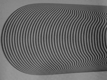
An example of the fringe pattern obtained with an oil drop entrained by the shear stress of a ZPG TBL is shown in figure 2. From this example it is evident that there exists considerable freedom for the practical determination of the fringe spacing as a function of time. To date, each experimental group has its own preferences which are rarely documented in publications: some use the region near the leading edge, others avoid it, some advocate using the early stages of drop evolution while others process only the late stages. In short, to choose the region and time for the analysis of interferograms which minimises the error of
 ${\it\tau}_{w}^{\ast }$
, the corrections to the basic Tanner and Blows theory need to be established. The analysis of all other sources of experimental error is of course also necessary (see e.g. Janke Reference Janke1993; Fernholz et al.
Reference Fernholz, Janke, Schober, Wagner and Warnack1996; Vinuesa et al.
Reference Vinuesa, Bartrons, Chiu, Dressler, Rüedi, Suzuki and Nagib2014), but will not be further discussed in this paper.
Example of an oil-drop interferogram. Flow is from left to right.

The most obvious shortcoming of the basic similarity solution (1.1) is the fact that, while it satisfies continuity of shear stress across the air–oil interface, the perturbation of the air boundary layer by a finite-thickness oil drop is neglected, corresponding to a velocity jump across the interface. Continuity of velocity induces a secondary air boundary layer above the oil drop which increases the shear stress imparted to the oil. Hence, if
 ${\it\tau}_{w}^{\ast }$
is extracted from interferograms according to (1.2), the wall shear stress of the air boundary layer without the oil drop is systematically overestimated. This error only disappears in the limit of
 $t\rightarrow \infty$
when the oil-drop height
 $h^{\ast }\rightarrow 0$
. Other sources of systematic errors, neglected in the basic theory (1.1), are deviations of the oil-drop shape from a perfect two-dimensional wedge, as well as the associated surface tension effects. In other words, the basic solution (1.1) constitutes a leading-order approximation for infinitesimally thin oil-film wedges and needs to be refined in order to quantify the systematic errors resulting from the interpretation of interferograms of finite-thickness oil drops with (1.2).
The paper is organised as follows. In § 2 corrections to the basic similarity solution of Tanner & Blows (Reference Tanner and Blows1976) and the corresponding equation (1.2) for the fringe spacing are derived for a ZPG TBL using a perturbation approach. The analysis is first validated in § 3 by comparison with a numerical solution of the linearised Reynolds-averaged Navier–Stokes (RANS) equations with different mixing-length models specially adapted to the near-wall region. In § 4 interferograms acquired in a laboratory set-up are presented and shown to be well described by the two-dimensional analysis of § 2. The final section, § 5, is devoted to a summary of the principal findings and to some recommendations for the optimal use of the oil-drop technique.
2. Asymptotic analysis of the shear-stress perturbation in a ZPG TBL caused by a thin two-dimensional oil film
For the following analysis, the oil drop is taken to be two-dimensional, an assumption which will be justified experimentally in § 4.1. The streamwise extent of the oil film is characterised by the distance
 $L^{\ast }$
between the drop leading edge and the point where it reaches a thickness
 $h^{\ast }$
of one viscous unit of the air boundary layer at the start of the observation, i.e.
 $h^{+}(L^{+},t=0)=1$
. In other words,
 $L^{+}$
is a measure of the inverse slope of the upstream part of the drop. At the same time, we assume that
 $L^{+}$
is also of the order of the streamwise distance over which interference fringes are monitored. Here, and in the following, the
 $+$
superscript indicates viscous boundary-layer scaling in air, i.e. normalisation with air density
 ${\it\rho}^{\ast }$
, kinematic viscosity
 ${\it\nu}^{\ast }$
and friction velocity
 $u_{{\it\tau}}^{\ast }$
, related to the unperturbed wall shear stress by
 ${\it\tau}_{w}^{\ast }={\it\rho}^{\ast }(u_{{\it\tau}}^{\ast })^{2}$
, while the
 $\ast$
superscript denotes dimensional quantities. Two additional parameters are required to characterise the oil drop: its maximum thickness
 $h_{max}^{+}$
at the start of observation and its total length
 $L_{max}^{+}$
. In the following, we will assume that the oil drop is entirely buried in the viscous sub-layer, i.e. that
 $h_{max}^{+}=\mathit{O}(1)$
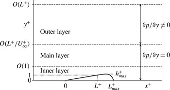
. The different parameters characterising the oil-drop geometry, together with the three layers required to analyse the effect of the drop on the air boundary layer in the following sections, are shown in figure 3.
Schematic of the layer structure for the asymptotic analysis. Flow is from left to right.

The analysis uses the two-dimensional (2D) unsteady RANS (abbreviated ‘URANS’) equations, which allow for a slow time dependence of the averaged flow quantities. In the following,
 $\langle \cdot \rangle$
denotes averaging of the turbulent correlations, while capital letters are used for the average velocity and pressure. The URANS equations are made dimensionless by scaling the streamwise, wall-normal and time coordinates as
 $$\begin{eqnarray}{\it\xi}=\frac{x^{\ast }}{L^{\ast }},\quad {\it\eta}=\frac{y^{\ast }-h^{\ast }({\it\xi})}{{\it\Delta}^{\ast }},\quad t=\frac{R_{{\it\mu}}u_{{\it\tau}}^{\ast }t^{\ast }}{L^{\ast }}.\end{eqnarray}$$
The normalisation of
 $x^{\ast }$
with
 $L^{\ast }$
provides the correct scaling of streamwise derivatives of perturbation quantities, while the unperturbed flow (the flow without the oil drop) is assumed independent of
 $x^{\ast }$
. This implies that the length of the observation area has to be much shorter than the characteristic evolution length
 $\mathit{Re}_{{\it\delta}_{\ast }}\,(U_{\infty }^{+})^{2}$
of the unperturbed ZPG TBL (Monkewitz, Chauhan & Nagib Reference Monkewitz, Chauhan and Nagib2007), where
 $\mathit{Re}_{{\it\delta}_{\ast }}=U_{\infty }^{\ast }{\it\delta}_{\ast }^{\ast }/{\it\nu}^{\ast }$
is the Reynolds number based on the displacement thickness,
 ${\it\delta}_{\ast }^{\ast }$
. In the following, the length of the observation window can be taken of
 $\mathit{O}(L^{+})$
, which automatically satisfies the above requirement due to the restriction
 $L^{+}\lesssim 0.1\,\mathit{Re}_{{\it\delta}_{\ast }}\,U_{\infty }^{+}$
imposed in § 2.2 in order to make analytical progress.
The wall-normal coordinate is shifted up by
 $h^{\ast }({\it\xi})$
so that
 ${\it\eta}=0$
corresponds to the oil–air interface. Such a uniform shift applied to the mixing-length model introduced in § 2.1 has essentially the effect of pushing the near-wall turbulent structures out of the way without distortion. As it will turn out, this leads to relatively minor shear-stress corrections at the oil–air interface. Any attenuation of the coordinate shift with increasing wall distance, (3.1), explored with the numerical experiments of § 3, will be seen to significantly increase the shear-stress correction. Finally, the limiting case of no
 $y^{\ast }$
-shift at all, considered in § 2.6 and corresponding physically to turbulence structures not reacting to the bump, is again amenable to asymptotic analysis and leads to a shear-stress correction which is an order of magnitude larger than the one obtained with the uniform shift of (2.1). The vertical scale
 ${\it\Delta}^{\ast }$
in (2.1) is left unspecified at this point as it has to be determined in each layer by the respective dominant balance of perturbation terms. Finally, the scaling of time is determined globally by the (slow) rate of oil-film thinning which, according to the leading-order equation (1.1) of Tanner & Blows (Reference Tanner and Blows1976), occurs on the characteristic scale
 $t_{thinning}^{\ast }=L^{\ast }/(R_{{\it\mu}}u_{{\it\tau}}^{\ast })$
, where
 $R_{{\it\mu}}={\it\mu}^{\ast }/{\it\mu}_{oil}^{\ast }$
is the typically very small dynamic viscosity ratio between air and oil.
The mean quantities and the Reynolds stresses are normalised as
 $$\begin{eqnarray}U^{+}=\frac{U^{\ast }}{u_{{\it\tau}}^{\ast }},\quad V=\frac{L^{+}}{{\it\Delta}^{+}}\frac{V^{\ast }}{u_{{\it\tau}}^{\ast }},\quad P=\frac{P^{\ast }}{{\it\tau}_{w}^{\ast }},\quad \langle u_{i}^{\prime }u_{j}^{\prime }\rangle ^{+}=\frac{\langle u_{i}^{\prime }u_{j}^{\prime }\rangle ^{\ast }}{(u_{{\it\tau}}^{\ast })^{2}}.\end{eqnarray}$$
With these normalisations, and neglecting
 ${\it\xi}$
-derivatives of the viscous and Reynolds stresses, the boundary-layer approximation of the URANS equations for
 ${\it\Delta}^{+}/L^{+}\ll 1$
reads
 $$\begin{eqnarray}\displaystyle & \displaystyle U_{{\it\xi}}^{+}+V_{{\it\eta}}=\frac{1}{{\it\Delta}^{+}}h_{{\it\xi}}^{+}U_{{\it\eta}}^{+}, & \displaystyle\end{eqnarray}$$
 $$\begin{eqnarray}\displaystyle & \displaystyle R_{{\it\mu}}U_{t}^{+}+U^{+}U_{{\it\xi}}^{+}+\left(V-\frac{U^{+}}{{\it\Delta}^{+}}h_{{\it\xi}}^{+}\right)U_{{\it\eta}}^{+}=-P_{{\it\xi}}+\frac{L^{+}}{{\it\Delta}^{+}}\left(\frac{1}{{\it\Delta}^{+}}U_{{\it\eta}}^{+}-\langle u^{\prime }v^{\prime }\rangle ^{+}\right)_{{\it\eta}}, & \displaystyle\end{eqnarray}$$
 $$\begin{eqnarray}\displaystyle & \displaystyle P_{{\it\eta}}=\mathit{O}\left(\frac{{\it\Delta}^{+}}{L^{+}}\right)^{2}+\mathit{O}\left(\frac{1}{L^{+}}\right)\ll 1. & \displaystyle\end{eqnarray}$$
 ${\it\Delta}^{+}/L^{+}=\mathit{O}(1)$
the above approximation is no longer valid and the full vertical momentum equation must be used. This situation arises only in the outer layer treated in § 2.3, where the appropriate equations are given.
In the oil layer, the Reynolds number (based on the oil height and maximum oil velocity) is
 $R_{{\it\nu}}R_{{\it\mu}}(h^{+})^{2}\ll 1$
(with
 $R_{{\it\nu}}={\it\nu}^{\ast }/{\it\nu}_{oil}^{\ast }$
) so that the oil motion is a laminar Couette–Poiseuille flow with velocity profile
 $$\begin{eqnarray}U_{oil}^{+}=R_{{\it\mu}}\left[{\it\tau}_{oil}y^{+}+\frac{1}{L^{+}}P_{{\it\xi}}y^{+}\left(\frac{y^{+}}{2}-h^{+}\right)\right].\end{eqnarray}$$
The coefficient
 ${\it\tau}_{oil}\equiv {\it\tau}_{oil}^{\ast }/{\it\tau}_{w}^{\ast }$
and the pressure gradient are unknowns and must be found from the matching of the shear stress and pressure gradient between air and oil. Only their limiting values
 ${\it\tau}_{oil}=1$
and
 $P_{{\it\xi}}=0$
are known for an infinitely thin drop in a ZPG boundary layer. The deviation from these limiting values for an oil drop of small but finite thickness is the subject of this paper. To describe the resulting wall-shear-stress perturbation, an approach similar to the triple-deck concept of Stewartson & Williams (Reference Stewartson and Williams1969) and its turbulent extension by Jackson & Hunt (Reference Jackson and Hunt1975) and Sykes (Reference Sykes1980) for low hills in the atmospheric boundary layer is adopted. The outer potential layer (see figure 3) is driven by the blowing velocity due to the drop and provides the streamwise pressure gradient in the main layer. The latter is assumed to lie within the logarithmic region of the unperturbed mean velocity profile where convection, turbulent diffusion and pressure gradient balance. Below the main layer, a constant-stress layer exists which is unaffected by the pressure gradient and acts like a ‘wall function’ for the main layer.
2.1. Inner-layer analysis
With
 $L^{+}\gg 1$
(2.4) reduces at leading order, within a layer of thickness
 ${\it\Delta}^{+}=\mathit{O}(1)$
, to the balance between viscous and Reynolds stresses (see also Mellor Reference Mellor1972). Hence
 ${\it\Delta}^{+}=1$
and
 ${\it\eta}=y^{+}-h^{+}$
in this inner layer. The streamwise mean velocity is decomposed as
 $$\begin{eqnarray}U^{+}=U_{B}^{+}({\it\eta})+{\rm\Delta}U({\it\xi},{\it\eta};L^{+}),\end{eqnarray}$$
where
 $U_{B}^{+}({\it\eta})$
is the basic undisturbed velocity profile and
 ${\rm\Delta}U$
the quasi-steady spatial velocity perturbation which depends parametrically on
 $L^{+}$
. Since
 $L^{+}\gg 1$
, the pressure gradient and the convective terms are of the same order and the streamwise momentum equation reduces to the balance between the viscous and Reynolds stresses, i.e.
 $$\begin{eqnarray}U_{{\it\eta}}^{+}-\langle u^{\prime }v^{\prime }\rangle ^{+}=1+{\it\tau},\end{eqnarray}$$
with
 ${\it\tau}$
the perturbation of the wall shear stress due to the oil drop. A similar result was also obtained by Sykes (Reference Sykes1980) for a taller hump. To proceed, a closure model for the Reynolds stress
 $\langle u^{\prime }v^{\prime }\rangle ^{+}$
is needed. For the present analysis, the simplest mixing-length model,
 $$\begin{eqnarray}-\langle u^{\prime }v^{\prime }\rangle ^{+}=(l_{m}^{+}\,U_{{\it\eta}}^{+})^{2}=({\it\kappa}{\it\eta}\,D\,U_{{\it\eta}}^{+})^{2},\end{eqnarray}$$
is adopted with
 ${\it\kappa}$
the von Kármán constant and
 $D$
a novel van-Driest-like correction factor
 $$\begin{eqnarray}D({\it\eta})=\{1-\exp [-(0.0086{\it\eta})^{2}-(0.02755{\it\eta})^{4}]\}^{1/4}.\end{eqnarray}$$
The modification of
 $D$
relative to the original van Driest factor (van Driest Reference van Driest1956) is designed to yield both the correct leading term of the Taylor expansion of the unperturbed
 $\langle u^{\prime }v^{\prime }\rangle$
and up-to-date log-law parameters. Equation (2.10) is motivated by the Taylor expansions of the unperturbed mean velocity and Reynolds stress, which are of the form
 $U_{B}^{+}=y^{+}-t_{4}^{(U)}(y^{+})^{4}+\cdots \,$
and
 $\langle u^{\prime }v^{\prime }\rangle ^{+}=-4t_{4}^{(U)}\,(y^{+})^{3}+\cdots \,$
, respectively, with the coefficient
 $t_{4}^{(U)}\approx 3.2\times 10^{-4}$
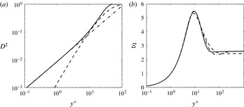
extracted from the direct numerical simulation (DNS) of Schlatter & Örlü (Reference Schlatter and Örlü2010). Figure 4(a) compares the new factor (2.10) to its Taylor expansion and the original van Driest factor, showing a significant improvement for
 $y^{+}$
of order unity where the oil–air interface is located. The indicator functions,
 ${\it\Xi}\equiv y^{+}(\text{d}U^{+}/\text{d}y^{+})$
, corresponding to the original van Driest factor and the new factor (2.10), are compared in figure 4(b) to the best fit of Monkewitz et al. (Reference Monkewitz, Chauhan and Nagib2007).
(a) ——, Modified factor (2.10); - - - -, original van Driest factor (van Driest Reference van Driest1956); – ⋅ – ⋅ –, leading term of the Taylor expansion obtained from DNS. (b) ——, Indicator function
 ${\it\Xi}\equiv y^{+}(\text{d}U^{+}/\text{d}y^{+})$
resulting from (2.11) with
 ${\it\kappa}=0.384$
and
 ${\it\tau}=0$
(unperturbed profile); - - - -, original van Driest model with
 ${\it\kappa}=0.41$
; – ⋅ – ⋅ –, fit of Monkewitz et al. (Reference Monkewitz, Chauhan and Nagib2007).

Assuming that the closure model (2.9) is only affected by the presence of the oil drop via the shift of origin of
 $y^{\ast }$
, (2.1), (2.8) and (2.9) immediately yield the total velocity derivative
 $$\begin{eqnarray}U_{{\it\eta}}^{+}=\frac{1}{2({\it\kappa}{\it\eta}D)^{2}}\left[\sqrt{1+4({\it\kappa}{\it\eta}D)^{2}(1+{\it\tau})}-1\right].\end{eqnarray}$$
For
 $y^{+}\rightarrow \infty$
, (2.11) integrates to
 $$\begin{eqnarray}U^{+}=\frac{\sqrt{1+{\it\tau}}}{{\it\kappa}}\ln {\it\eta}+B_{1}+b_{0}\quad ({\it\eta}\rightarrow \infty ),\end{eqnarray}$$
where
 $B_{1}$
is determined from the integral of (2.11) and
 $b_{0}$
is a function which must be found from the matching of the streamwise velocity between air and oil. Since the basic mean flow in the inner layer asymptotes to
 $U_{B}^{+}={\it\kappa}^{-1}\ln {\it\eta}+B$
for
 $y^{+}\rightarrow \infty$
, the streamwise perturbation velocity asymptotes to
 $$\begin{eqnarray}{\rm\Delta}U=U^{+}-U_{B}^{+}=\frac{\sqrt{1+{\it\tau}}-1}{{\it\kappa}}\ln {\it\eta}+(B_{1}-B)+b_{0}\quad ({\it\eta}\rightarrow \infty ),\end{eqnarray}$$
where
 $B_{1}-B={\it\sigma}{\it\tau}\equiv 5.795{\it\tau}$
is the variation of the logarithmic intercept due to the shear-stress perturbation
 ${\it\tau}$
.
At the lower edge of the inner layer, as
 ${\it\eta}\rightarrow 0$
,
 $U_{{\it\eta}}^{+}\rightarrow 1+{\it\tau}+\mathit{O}({\it\eta}^{3})$
, and the total streamwise velocity near the wall is
 $U^{+}=b_{0}+(1+{\it\tau}){\it\eta}+\mathit{O}({\it\eta}^{4})$
. Matching shear stress and streamwise velocity at the air–oil interface yields
 $$\begin{eqnarray}{\it\tau}_{oil}=1+{\it\tau}\quad \text{and}\quad b_{0}=R_{{\it\mu}}(1+{\it\tau})h^{+}.\end{eqnarray}$$
Here, pressure gradients have been neglected (to be justified a posteriori), which makes the oil flow a pure Couette flow driven by the undisturbed wall shear plus a perturbation
 ${\it\tau}$
. The latter must be determined from the matching to the upper layers where, in particular, the logarithmic increase of the perturbation velocity (2.13) is arrested. The slip velocity
 $b_{0}$
is of
 $\mathit{O}(R_{{\it\mu}})$
. For typical values of
 $L^{+}$
and
 $R_{{\it\mu}}\lesssim 10^{-4}$
,
 $b_{0}$
is much smaller than
 $(1/L^{+})$
and can therefore be neglected in the determination of the wall-shear-stress perturbation, making the oil drop essentially a rigid bump.
2.2. Main-layer analysis
At the top of the inner region the viscous effects vanish and in the following main layer the Reynolds-stress term is balanced by the inertial terms. The characteristic thickness of this main layer is
 ${\it\Delta}_{m}$
, for the moment still undefined, and the associated scaled wall-normal coordinate is
 ${\it\eta}\equiv Y=(y^{+}-h^{+})/{\it\Delta}_{m}^{+}$
. For the following, we assume that the undisturbed mean velocity profile is logarithmic throughout this layer, corresponding to a mixing length which is linear in
 $Y$
. The requirement that the deviation from the log law be
 $\mathit{O}(1)$
at the outer edge of the main layer imposes a first limitation on
 ${\it\Delta}_{m}^{+}$
, namely
 ${\it\Delta}_{m}^{+}\lesssim 0.1\mathit{Re}_{{\it\delta}_{\ast }}$
. This assumption allows the mean velocity profile to be decomposed as
 $$\begin{eqnarray}U_{B}^{+}=U_{\infty }^{+}-W(Y)=\frac{1}{{\it\kappa}}\ln {\it\Delta}_{m}^{+}+\frac{1}{{\it\kappa}}\ln Y+B,\end{eqnarray}$$
so that
 $$\begin{eqnarray}W(Y)=U_{\infty }^{+}-\frac{1}{{\it\kappa}}\ln {\it\Delta}_{m}^{+}-B-\frac{1}{{\it\kappa}}\ln Y=C-B-\frac{1}{{\it\kappa}}\ln Y,\end{eqnarray}$$
with
 $C=U_{\infty }^{+}-{\it\kappa}^{-1}\ln {\it\Delta}_{m}^{+}=\mathit{O}(1)$
a constant.
The following perturbation expansions are introduced:
 $$\begin{eqnarray}\displaystyle & \displaystyle U^{+}=U_{\infty }^{+}-W(Y)+{\it\omega}_{m}\left(U_{1}+\frac{1}{U_{\infty }^{+}}U_{2}\right), & \displaystyle\end{eqnarray}$$
 $$\begin{eqnarray}\displaystyle & \displaystyle V=\frac{1}{{\it\Delta}_{m}^{+}}h_{{\it\xi}}^{+}U^{+}+{\it\omega}_{m}\left(V_{1}+\frac{1}{U_{\infty }^{+}}V_{2}\right), & \displaystyle\end{eqnarray}$$
 $$\begin{eqnarray}\displaystyle & \displaystyle P={\it\omega}_{p}\left(P_{1}+\frac{1}{U_{\infty }^{+}}P_{2}\right), & \displaystyle\end{eqnarray}$$
 ${\it\omega}_{m}$
and
 ${\it\omega}_{p}$
are the, as yet unknown, orders of magnitude of the velocity and pressure perturbations. With this, the linearised streamwise momentum equation takes the form
 $$\begin{eqnarray}\displaystyle & & \displaystyle (U_{\infty }^{+}-W)\left(U_{1,{\it\xi}}+\frac{1}{U_{\infty }^{+}}U_{2,{\it\xi}}\right)-W_{Y}V_{1}\nonumber\\ \displaystyle & & \displaystyle =-\frac{{\it\omega}_{p}}{{\it\omega}_{m}}\left(P_{1,{\it\xi}}+\frac{1}{U_{\infty }^{+}}P_{2,{\it\xi}}\right)+2{\it\kappa}\frac{L^{+}}{{\it\Delta}_{m}^{+}}\left(YU_{1,Y}+\frac{1}{U_{\infty }^{+}}YU_{2,Y}\right)_{Y}.\end{eqnarray}$$
In the main layer the convective and Reynolds-stress terms are of the same order as the pressure terms, so that
 ${\it\omega}_{m}={\it\omega}_{p}/U_{\infty }^{+}$
and
 ${\it\Delta}_{m}^{+}=L^{+}/U_{\infty }^{+}$
. Grouping the terms of
 $\mathit{O}(U_{\infty }^{+})$
and
 $\mathit{O}(1)$
yields at leading order
 $$\begin{eqnarray}\displaystyle & U_{1,{\it\xi}}+V_{1,Y}=0, & \displaystyle\end{eqnarray}$$
 $$\begin{eqnarray}\displaystyle & U_{1,{\it\xi}}=-P_{1,{\it\xi}}+2{\it\kappa}(YU_{1,Y})_{Y}, & \displaystyle\end{eqnarray}$$
 $$\begin{eqnarray}\displaystyle & U_{2,{\it\xi}}+V_{2,Y}=0, & \displaystyle\end{eqnarray}$$
 $$\begin{eqnarray}\displaystyle & U_{2,{\it\xi}}-WU_{1,{\it\xi}}-W_{Y}V_{1}=-P_{2,{\it\xi}}+2{\it\kappa}(YU_{2,Y})_{Y}. & \displaystyle\end{eqnarray}$$
 $P_{2,Y}=\mathit{O}(U_{\infty }^{+})^{-1}$
, the wall-normal pressure gradient is zero up to the second order, while the third-order problem will necessarily involve
 $P_{3,Y}\neq 0$
.
Applying the streamwise Fourier transform defined by
 $$\begin{eqnarray}\widehat{F}({\it\alpha})=\int _{\mathbb{R}}F({\it\xi})\text{e}^{-\text{i}{\it\alpha}{\it\xi}}\,\text{d}{\it\xi},\end{eqnarray}$$
to (2.22) yields
 $$\begin{eqnarray}\widehat{U}_{1}=-\widehat{P}_{1}+\frac{2{\it\kappa}}{\text{i}{\it\alpha}}(Y\widehat{U}_{1,Y})_{Y}.\end{eqnarray}$$
With the transformation
 $z=\sqrt{2\text{i}{\it\alpha}Y/{\it\kappa}}$
, (2.26) becomes an inhomogeneous modified Bessel equation (Abramowitz & Stegun Reference Abramowitz and Stegun1972; Jackson & Hunt Reference Jackson and Hunt1975), with the solution
 $$\begin{eqnarray}\widehat{U}_{1}=\widehat{c}_{1}K_{0}(z)+\widehat{c}_{2}I_{0}(z)-\widehat{P}_{1},\end{eqnarray}$$
where
 $\widehat{c}_{1}$
and
 $\widehat{c}_{2}$
are unknown functions and
 $I_{0}$
and
 $K_{0}$
the modified Bessel functions of the first and second kind, respectively. As
 $I_{0}\rightarrow \infty$
for
 $Y\rightarrow \infty$
,
 $c_{2}=0$
to ensure boundedness of the solution. Since
 $K_{0}(z)$
has a logarithmic behaviour for
 $z\rightarrow 0$
which cannot be matched with the inner layer at this order, one must have also
 $c_{1}=0$
. Therefore, the first-order velocity correction is simply
 $U_{1}=-P_{1}$
, with the corresponding wall-normal velocity given by
 $V_{1}=P_{1,{\it\xi}}Y+V_{1}(0)$
. To avoid unnecessary complications, it is also anticipated that
 $V_{1}(0)=\mathit{O}(L^{+})^{-1}=0$
, i.e. that the blowing velocity at the bottom of the main layer is negligible, as shown in § 2.5.
The equation for the second-order problem is the same as (2.27) but with additional inhomogeneities. After some algebra, its solution is obtained as
 $$\begin{eqnarray}\widehat{U}_{2}=\widehat{d}_{1}K_{0}(z)-\widehat{P}_{2}-\widehat{P}_{1}\left[K_{0}(z)\int _{0}^{z}qI_{0}(q){\it\Phi}\!\left(\frac{{\it\kappa}q^{2}}{2\text{i}{\it\alpha}}\right)\text{d}q+I_{0}(z)\int _{z}^{\infty }qK_{0}(q){\it\Phi}\left(\frac{{\it\kappa}q^{2}}{2\text{i}{\it\alpha}}\right)\text{d}q\right],\end{eqnarray}$$
where
 ${\it\Phi}(Y)=W-YW_{Y}$
. Note that the solution (2.28) does not grow exponentially as
 $Y\rightarrow \infty$
even though
 $I_{0}(z)$
does.
Collecting the above results, the perturbation velocities in the limit of large
 $Y$
are
 $$\begin{eqnarray}\displaystyle & \displaystyle \widehat{{\rm\Delta}U}^{+}=-{\it\omega}_{m}\left\{\widehat{P}_{1}+\frac{1}{U_{\infty }^{+}}[\widehat{P}_{2}+(W-YW_{Y})\widehat{P}_{1}]\right\}, & \displaystyle\end{eqnarray}$$
 $$\begin{eqnarray}\displaystyle & \displaystyle \widehat{V}=\frac{\text{i}{\it\alpha}\widehat{h}^{+}}{{\it\Delta}_{m}^{+}}(U_{\infty }^{+}-W)+\text{i}{\it\alpha}{\it\omega}_{m}\left[\widehat{P}_{1}Y+\frac{1}{U_{\infty }^{+}}\left(\widehat{P}_{2}Y+\widehat{P}_{1}\int _{0}^{Y}{\it\Phi}(q)\,\text{d}q+D\right)\right], & \displaystyle\end{eqnarray}$$
 $D$
an integration constant.
On the other hand, as
 $Y\rightarrow 0$
, the streamwise velocity perturbation behaves as
 $$\begin{eqnarray}\widehat{{\rm\Delta}U}^{+}=-{\it\omega}_{m}\left\{\widehat{P}_{1}+\frac{1}{U_{\infty }^{+}}\left[-\widehat{d}_{1}K_{0}(z)+\widehat{P}_{2}+\widehat{P}_{1}\int _{0}^{\infty }qK_{0}(q){\it\Phi}\left(\frac{{\it\kappa}q^{2}}{2\text{i}{\it\alpha}}\right)\,\text{d}q\right]\right\},\end{eqnarray}$$
with the modified Bessel function behaving at small
 $Y$
as
 $$\begin{eqnarray}K_{0}(z)\sim -\left[{\it\gamma}+\ln \left(\frac{z}{2}\right)\right]=-\left[{\it\gamma}+\ln \sqrt{\frac{\text{i}{\it\alpha}}{2{\it\kappa}}}+\frac{1}{2}\ln (Y)\right],\end{eqnarray}$$
with
 ${\it\gamma}=0.577\dots$
the Euler–Mascheroni constant. The integral in (2.31) can be evaluated for small
 $Y$
:
 $$\begin{eqnarray}\int _{0}^{\infty }qK_{0}{\it\Phi}\left(\frac{{\it\kappa}q^{2}}{2\text{i}{\it\alpha}}\right)\,\text{d}q=C-B+\frac{1}{{\it\kappa}}\left(1+\ln \frac{2\text{i}{\it\alpha}}{{\it\kappa}}\right)-\frac{2}{{\it\kappa}}{\it\chi},\end{eqnarray}$$
with
 ${\it\chi}=\int _{0}^{\infty }qK_{0}(q)\ln q\,\text{d}q\approx 0.1159$
.
A consequence of (2.29) and (2.31) is that the streamwise velocity perturbation behaves logarithmically (at second order) both close to the wall, where it has to be matched with the inner layer, and for
 $Y\rightarrow \infty$
. On the other hand, the wall-normal velocity goes to zero close to the wall. For large
 $Y$
, it exhibits a linear increase with
 $Y$
plus the term
 ${\it\alpha}\widehat{h}^{+}U^{+}/{\it\Delta}_{m}^{+}$
, which is the blowing velocity directly induced by the topology of the oil drop.
2.3. Outer-layer analysis
In the outer region the perturbation pressure has to decay to zero towards the free stream. Therefore, this region must have an aspect ratio of one in order to obtain an elliptic equation for the perturbation. Hence the outer layer has a thickness
 ${\it\Delta}^{+}=L^{+}$
. Furthermore, since its lower edge is far enough from the wall, the upward shift by
 $h^{+}$
of the wall-normal coordinate is no longer necessary. Hence, the wall-normal coordinate in the outer layer is
 $$\begin{eqnarray}{\it\zeta}=y^{+}/L^{+}.\end{eqnarray}$$
With the perturbation expansions
 $$\begin{eqnarray}\displaystyle & \displaystyle U^{+}=U_{\infty }^{+}-W({\it\zeta})+{\it\omega}_{u}\left(U_{1}+\frac{1}{U_{\infty }^{+}}U_{2}\right), & \displaystyle\end{eqnarray}$$
 $$\begin{eqnarray}\displaystyle & \displaystyle V^{+}={\it\omega}_{u}\left(V_{1}+\frac{1}{U_{\infty }^{+}}V_{2}\right), & \displaystyle\end{eqnarray}$$
 $$\begin{eqnarray}\displaystyle & \displaystyle P^{+}={\it\omega}_{p}\left(P_{1}+\frac{1}{U_{\infty }^{+}}P_{2}\right), & \displaystyle\end{eqnarray}$$
 $$\begin{eqnarray}\displaystyle & \displaystyle (U_{\infty }^{+}-W)\!\left(U_{1,{\it\xi}}+\frac{1}{U_{\infty }^{+}}U_{2,{\it\xi}}\right)-W_{{\it\zeta}}V_{1}=-\frac{{\it\omega}_{p}}{{\it\omega}_{u}}\left(P_{1,{\it\xi}}+\frac{1}{U_{\infty }^{+}}P_{2,{\it\xi}}\right)\!+({\it\psi}U_{1,{\it\zeta}})_{{\it\zeta}}, & \displaystyle\end{eqnarray}$$
 $$\begin{eqnarray}\displaystyle & \displaystyle (U_{\infty }^{+}-W)\left(V_{1,{\it\xi}}+\frac{1}{U_{\infty }^{+}}V_{2,{\it\xi}}\right)=-\frac{{\it\omega}_{p}}{{\it\omega}_{u}}\left(P_{1,{\it\zeta}}+\frac{1}{U_{\infty }^{+}}P_{2,{\it\zeta}}\right), & \displaystyle\end{eqnarray}$$
 ${\it\psi}=-2l_{m}^{2}W_{{\it\zeta}}\rightarrow 2{\it\kappa}{\it\zeta}$
as
 ${\it\zeta}\rightarrow 0$
. Grouping the terms of
 $\mathit{O}(U_{\infty }^{+})$
and
 $\mathit{O}(1)$
leads at leading order to
 $$\begin{eqnarray}\displaystyle & U_{1,{\it\xi}}+V_{1,{\it\zeta}}=0, & \displaystyle\end{eqnarray}$$
 $$\begin{eqnarray}\displaystyle & U_{1,{\it\xi}}=-P_{1,{\it\xi}}, & \displaystyle\end{eqnarray}$$
 $$\begin{eqnarray}\displaystyle & V_{1,{\it\xi}}=-P_{1,{\it\zeta}}, & \displaystyle\end{eqnarray}$$
 $$\begin{eqnarray}\displaystyle & U_{2,{\it\xi}}+V_{2,{\it\zeta}}=0, & \displaystyle\end{eqnarray}$$
 $$\begin{eqnarray}\displaystyle & U_{2,{\it\xi}}-WU_{1,{\it\xi}}-W_{{\it\zeta}}V_{1}=-P_{2,{\it\xi}}+({\it\psi}U_{1,{\it\zeta}})_{{\it\zeta}}, & \displaystyle\end{eqnarray}$$
 $$\begin{eqnarray}\displaystyle & V_{2,{\it\xi}}-WV_{1,{\it\xi}}=-P_{2,{\it\zeta}}. & \displaystyle\end{eqnarray}$$
 $$\begin{eqnarray}\displaystyle & {\rm\nabla}^{2}V_{1}=V_{1,{\it\xi}{\it\xi}}+V_{1,{\it\zeta}{\it\zeta}}=0, & \displaystyle\end{eqnarray}$$
 $$\begin{eqnarray}\displaystyle & {\rm\nabla}^{2}V_{2}=-W_{{\it\zeta}{\it\zeta}}V_{1}-({\it\psi}U_{1,{\it\zeta}})_{{\it\zeta}{\it\zeta}}=H({\it\xi},\,{\it\zeta}). & \displaystyle\end{eqnarray}$$
The solution of the Laplace equation (2.46) is readily found in terms of the Fourier transform
 $$\begin{eqnarray}\widehat{V}_{1}=\widehat{{\it\Gamma}}\text{e}^{-|{\it\alpha}|{\it\zeta}},\end{eqnarray}$$
while the solution of the second-order problem (2.47) is
 $$\begin{eqnarray}\displaystyle \widehat{V}_{2} & = & \displaystyle \widehat{{\it\Omega}}\text{e}^{-|{\it\alpha}|{\it\zeta}}+\frac{1}{{\it\alpha}}\int _{{\it\zeta}}^{\infty }\widehat{H}\sinh [{\it\alpha}(z-{\it\zeta})]\,\text{d}z=\widehat{{\it\Omega}}\text{e}^{-|{\it\alpha}|{\it\zeta}}-W\widehat{V}_{1}\nonumber\\ \displaystyle & & \displaystyle +\,2|{\it\alpha}|\widehat{{\it\Gamma}}\text{e}^{|{\it\alpha}|{\it\zeta}}\!\int _{{\it\zeta}}^{\infty }\!W\text{e}^{-2|{\it\alpha}|z}\,\text{d}z-{\it\psi}\widehat{U}_{1,{\it\zeta}}-{\it\alpha}\!\int _{{\it\zeta}}^{\infty }\!{\it\psi}\widehat{U}_{1,z}\sinh [{\it\alpha}(z-{\it\zeta})]\,\text{d}z.\end{eqnarray}$$
Consequently, at the bottom of the upper layer
 $({\it\zeta}\rightarrow 0)$
the wall-normal velocity approaches
 $$\begin{eqnarray}\widehat{V}^{+}={\it\omega}_{u}\widehat{{\it\Gamma}}+\frac{{\it\omega}_{u}}{U_{\infty }^{+}}\left[\widehat{{\it\Omega}}-W\widehat{{\it\Gamma}}+2|{\it\alpha}|\widehat{{\it\Gamma}}\int _{0}^{\infty }W\text{e}^{-2|{\it\alpha}|z}\,\text{d}z-{\it\alpha}\int _{0}^{\infty }{\it\psi}\widehat{U}_{1,z}\sinh ({\it\alpha}z)\,\text{d}z\right],\end{eqnarray}$$
while the pressure (for
 ${\it\zeta}\rightarrow 0$
) is
 $\widehat{P}_{1}=\text{i}\,\text{sgn}({\it\alpha})\widehat{{\it\Gamma}}$
at leading order and
 $$\begin{eqnarray}\widehat{P}_{2}=\text{i}\,\text{sgn}({\it\alpha})\left[\widehat{{\it\Omega}}-2|{\it\alpha}|\widehat{{\it\Gamma}}\int _{0}^{\infty }W\text{e}^{-2|{\it\alpha}|z}\,\text{d}z-|{\it\alpha}|\int _{0}^{\infty }{\it\psi}\widehat{U}_{1,z}\cosh ({\it\alpha}z)\,\text{d}z\right]\end{eqnarray}$$
at second order.
At this point, the structure of the perturbation solution emerges clearly: the upper layer is driven by the blowing velocity generated by the drop topology and transmitted through the two lower layers, and providing in turn the streamwise pressure gradient that drives the main layer. The resulting streamwise velocity perturbation in the main layer is logarithmic throughout the layer, while the wall-normal velocity vanishes towards the wall so that the main function of the inner layer is to impose the no-slip boundary condition at the oil–air interface.
2.4. Matching main and outer layers
By matching the wall-normal velocity at the top of the main layer (2.30) with the one at the bottom of the upper layer (2.50), one obtains the order of magnitude of the perturbations in the upper layer
 $$\begin{eqnarray}{\it\omega}_{u}={\it\omega}_{m}=\frac{U_{\infty }^{+}}{L^{+}},\quad {\it\omega}_{p}=\frac{(U_{\infty }^{+})^{2}}{L^{+}},\end{eqnarray}$$
and their wavenumber dependence
 $$\begin{eqnarray}\displaystyle & \displaystyle \widehat{{\it\Gamma}}=\text{i}{\it\alpha}\widehat{h}^{+}, & \displaystyle\end{eqnarray}$$
 $$\begin{eqnarray}\displaystyle & \displaystyle \widehat{{\it\Omega}}=-2|{\it\alpha}|\widehat{{\it\Gamma}}\int _{0}^{\infty }W\text{e}^{-2|{\it\alpha}|z}\,\text{d}z+{\it\alpha}\int _{0}^{\infty }{\it\psi}\widehat{U}_{1,z}\sinh ({\it\alpha}z)\,\text{d}z. & \displaystyle\end{eqnarray}$$
From the scalings (2.52) it can now be shown that the boundary condition for the vertical velocity at the bottom of the main layer is indeed
 $V_{1}(0)=0$
, as already anticipated in § 2.2. This follows from the normalisation (2.2) as the vertical velocity is of
 $\mathit{O}(L^{+})^{-1}$
in lower-layer scales and becomes
 $\mathit{O}({\it\Delta}_{m}^{+}L^{+})^{-1}\ll \mathit{O}({\it\omega}_{m})$
in main-layer scales.
Finally, (2.53) and (2.54) allow (2.51) for the pressure to be simplified to
 $$\begin{eqnarray}\widehat{P}_{2}=-\text{i}\,{\it\alpha}\left(4\widehat{{\it\Gamma}}\int _{0}^{\infty }W\text{e}^{-2|{\it\alpha}|z}\,\text{d}z+\int _{0}^{\infty }{\it\psi}\widehat{U}_{1,z}\text{e}^{-|{\it\alpha}|z}\,\text{d}z\right).\end{eqnarray}$$
2.5. Matching inner and main layers
The matching of the streamwise velocity in the inner layer as
 ${\it\eta}\rightarrow \infty$
(2.13) to the one in the main layer as
 $Y\rightarrow 0$
(2.31) yields
 $$\begin{eqnarray}\displaystyle & & \displaystyle -\frac{1}{L^{+}}\left(\frac{1}{{\it\kappa}}\ln {\it\Delta}_{m}^{+}+C\right)\widehat{P}_{1}-\frac{1}{L^{+}}\left[\widehat{d}_{1}\left({\it\gamma}+\ln \sqrt{\frac{\text{i}{\it\alpha}}{2{\it\kappa}}}+\frac{1}{2}\ln Y\right)+\widehat{P}_{2}\right.\nonumber\\ \displaystyle & & \displaystyle \qquad \left.+\,\widehat{P}_{1}\int _{0}^{\infty }{\it\eta}K_{0}{\it\Phi}\left(\frac{{\it\kappa}{\it\eta}^{2}}{2\text{i}{\it\alpha}}\right)\,\text{d}{\it\eta}\right]=\frac{\widehat{{\it\tau}}}{2{\it\kappa}}\ln {\it\Delta}_{m}^{+}+\frac{\widehat{{\it\tau}}}{2{\it\kappa}}\ln Y+{\it\sigma}\widehat{{\it\tau}}+\widehat{b_{0}},\end{eqnarray}$$
where
 $U_{\infty }^{+}$
in
 ${\it\omega}_{u}$
has been replaced by
 $U_{\infty }^{+}={\it\kappa}^{-1}\ln {\it\Delta}_{m}^{+}+C$
already used in (2.16). Furthermore, since
 $\mathit{O}(R_{{\it\mu}}{\it\tau})$
is negligible, the slip velocity
 $b_{0}=R_{{\it\mu}}(1+{\it\tau})h^{+}$
can be approximated by
 $b_{0}\approx R_{{\it\mu}}h^{+}$
to avoid a nonlinear term.
The matching of (2.56) at
 $\mathit{O}({\it\omega}_{m})$
and
 $\mathit{O}({\it\omega}_{m}/U_{\infty }^{+})$
leads to
 $\widehat{d}_{1}=2\widehat{P}_{1}/{\it\kappa}$
and
 $$\begin{eqnarray}\displaystyle \widehat{{\it\tau}} & = & \displaystyle -\frac{2}{L^{+}}\left\{\widehat{P}_{1}+\frac{{\it\kappa}}{\ln {\it\Delta}_{m}^{+}}\left[\widehat{P}_{2}+\widehat{P}_{1}\left(C+\frac{2{\it\gamma}}{{\it\kappa}}-2{\it\sigma}+\frac{2}{{\it\kappa}}\ln \sqrt{\frac{\text{i}{\it\alpha}}{2{\it\kappa}}}\right.\right.\right.\nonumber\\ \displaystyle & & \displaystyle \left.\left.\left.+\,\int _{0}^{\infty }{\it\eta}K_{0}{\it\Phi}\left(\frac{{\it\kappa}{\it\eta}^{2}}{2\text{i}{\it\alpha}}\right)\,\text{d}{\it\eta}\right)+L^{+}R_{{\it\mu}}\widehat{h}^{+}\right]\right\},\end{eqnarray}$$
where the product
 $L^{+}R_{{\it\mu}}$
has been assumed to be
 $\mathit{O}(1)$
. This is realistic in most practical applications but the result (2.57) also remains valid for
 $L^{+}R_{{\it\mu}}\ll 1$
.
Equation (2.57) concludes the analysis of the shear-stress perturbation acting on the oil film using a shifted wall-normal coordinate (2.1). Its principal feature is the appearance of the pressure perturbation
 $\widehat{P}_{1}$
at leading order which is the hallmark of an interactive triple deck.
2.6. Result without shifting the wall-normal coordinate
An analogous analysis has also been carried out without shifting the
 $y$
-coordinate, i.e. by using in all the layers
 $$\begin{eqnarray}{\it\eta}=\frac{y^{\ast }}{{\it\Delta}^{\ast }}\end{eqnarray}$$
instead of (2.1). The scales
 ${\it\Delta}^{+}$
remain the same for all the layers. The modified velocity boundary condition at the oil–air interface is obtained by Taylor expanding the total velocity around
 ${\it\eta}=0$
, leading to
 $u^{+}({\it\xi},{\it\eta}=0)=-h^{+}$
. However, the boundary condition for the Reynolds stress cannot be imposed. From the Taylor expansion of
 $\langle u^{\prime }v^{\prime }\rangle ^{+}$
given in § 2.1, the error is
 $\langle u^{\prime }v^{\prime }\rangle ^{+}(y^{+}=h^{+})=-1.28\times 10^{-3}\,(h^{+})^{3}$
, which is small compared to the maximum Reynolds stress, but significant in comparison with the stress perturbation.
This unshifted problem is amenable to a perturbation solution along the same lines as the analysis of §§ 2.1–2.5. The main differences are the value of
 $b_{0}\approx -(1+{\it\tau})h^{+}$
in the lower layer and a stress perturbation which becomes of
 $\mathit{O}(\ln {\it\Delta}_{m}^{+})^{-1}\gg \mathit{O}(L^{+})^{-1}$
, much larger than the perturbation obtained with the shifted coordinate of (2.1). As a result, the pressure perturbation is pushed up to higher-perturbation orders, corresponding to
 $P_{1}=P_{2}={\it\Gamma}={\it\Omega}=0$
but
 $\widehat{d}_{1}\neq 0$
in § 2.2 and the three layers become non-interactive. Because of the violation of the Reynolds-stress boundary condition, the value of this analysis is somewhat uncertain and only the final result corresponding to (2.57) is given here:
 $$\begin{eqnarray}\widehat{{\it\tau}}=\frac{2{\it\kappa}\widehat{h}^{+}}{\ln {\it\Delta}_{m}^{+}}+\frac{{\it\kappa}}{\ln ^{2}{\it\Delta}_{m}^{+}}\left[\left(4{\it\gamma}-4{\it\sigma}{\it\kappa}\right)\widehat{h}^{+}+5{\it\kappa}\widehat{h^{2}}^{+}+4\widehat{h}^{+}\ln \sqrt{\frac{\text{i}{\it\alpha}}{2{\it\kappa}}}\right]\!.\end{eqnarray}$$
The difference between the result (2.57), corresponding essentially to turbulence structures being pushed up by the oil drop without distortion, and (2.59), corresponding to turbulence structures not reacting to the presence of the drop, turns out to be significant. For the typical oil-film interferometry (OFI) parameters in the examples of § 3 (see figures 7 and 9), the perturbation shear stresses differ by an order of magnitude! The question of whether the solution (2.59) is meaningful despite the violation of the Reynolds-stress boundary condition will be answered positively in § 3 by numerical RANS simulations with the non-uniform coordinate shift (3.1).
2.7.
 $h^{+}$
distribution

For the application under consideration, the oil-height distribution is the relevant quantity since it determines directly the fringe spacing. From the continuity of the oil film, the evolution of
 $h^{\ast }$
is obtained as
 $$\begin{eqnarray}\frac{\partial h^{\ast }}{\partial t^{\ast }}=-\frac{\partial }{\partial x^{\ast }}\int _{0}^{h^{\ast }(x^{\ast })}U_{oil}^{\ast }(x^{\ast },y^{\ast })\,\text{d}y^{\ast },\end{eqnarray}$$
or in non-dimensional variables
 $$\begin{eqnarray}h_{t}^{+}=-\left[(h^{+})^{2}\frac{(1+{\it\tau})}{2}-\frac{P_{{\it\xi}}}{3L^{+}}(h^{+})^{3}\right]_{{\it\xi}}\approx -\left[(h^{+})^{2}\frac{(1+{\it\tau})}{2}\right]_{{\it\xi}}.\end{eqnarray}$$
According to the experimental observations, over a large upstream part of the oil drop
 $h^{+}$
is very nearly a linear function of
 ${\it\xi}$
. Therefore,
 $h^{+}$
is decomposed into a dominant linear term and a small corrective term, i.e.
 $h^{+}\sim h_{0}^{+}+h_{1}^{+}$
, with
 $h_{0}^{+}$
and
 $h_{1}^{+}$
determined by the differential equations
 $$\begin{eqnarray}h_{0,t}^{+}=-h_{0}^{+}h_{0,{\it\xi}}^{+}\end{eqnarray}$$
and
 $$\begin{eqnarray}h_{1,t}^{+}=-\left[h_{0}^{+}h_{1}^{+}+{\textstyle \frac{1}{2}}(h_{0}^{+})^{2}{\it\tau}\right]_{{\it\xi}}.\end{eqnarray}$$
With the Ansatz
 $h_{0}^{+}={\it\phi}(t){\it\xi}$
and the initial condition
 ${\it\phi}(0)=1$
imposed by the definition of
 $L^{+}$
, the solution of (2.62) is
 ${\it\phi}(t)=(1+t)^{-1}$
, providing the rate of decay of the slope of the front part of the oil film. Equation (2.62) is a nonlinear wave equation with general solution
 $h_{0}^{+}({\it\xi},t)=H({\it\xi}-h_{0}^{+}t)$
for any given initial drop shape
 $h_{0}^{+}({\it\xi},0)=H({\it\xi})$
. This implicit solution has, however, some drawbacks near the oil-drop trailing edge which is fixed in space and steepens until a Rankine–Hugoniot discontinuity is met, which then starts travelling downstream to conserve the oil volume. As this scenario is not realistic, the oil-drop shape is prescribed here as
 $$\begin{eqnarray}h_{0}^{+}({\it\xi},\,t)={\it\phi}\left[{\it\xi}-{\it\xi}_{f}\left(\frac{{\it\xi}}{{\it\xi}_{f}}\right)^{n}\right]\quad \text{with }{\it\phi}=\frac{1}{1+t},\end{eqnarray}$$
where
 ${\it\xi}_{f}$
and
 $n$
are functions of time. Requiring that the trailing-edge slope
 $-s$
, i.e. the advancing contact angle, as well as the drop volume remain constant leads to
 $$\begin{eqnarray}{\it\xi}_{f}(t)={\it\xi}_{f}(0)\sqrt{\frac{s+2{\it\phi}}{{\it\phi}(s+2)}},\quad n=1+\frac{s}{{\it\phi}}.\end{eqnarray}$$
A solution of (2.63) can be found in terms of characteristic curves. The first characteristic coordinate
 $s=t$
is obtained from the equation
 $t_{s}=1$
, while the equation
 ${\it\xi}_{s}=h_{0}^{+}$
determines the second characteristic coordinate
 $q$
,
 $$\begin{eqnarray}{\it\xi}=q+\int _{0}^{t}h_{0}^{+}[{\it\xi}(q,s),s]\,\text{d}s.\end{eqnarray}$$
In terms of these characteristic coordinates, (2.63) becomes
 $$\begin{eqnarray}h_{1,s}^{+}=-h_{1}^{+}h_{0,{\it\xi}}^{+}-Q\quad \text{with}~Q={\textstyle \frac{1}{2}}[(h_{0}^{+})^{2}{\it\tau}]_{{\it\xi}}.\end{eqnarray}$$
The solution of (2.67) is
 $$\begin{eqnarray}h_{1}^{+}(q,s)=\left[h_{1}^{+}(q,0)-\int _{0}^{s}Q\exp \left(\int _{0}^{r}h_{0,{\it\xi}}^{+}\,\text{d}w\right)\,\text{d}r\right]\exp \left(-\int _{0}^{s}h_{0,{\it\xi}}^{+}\,\text{d}w\right),\end{eqnarray}$$
where the integrals must be performed along the characteristics
 $q=\text{constant}$
.
Since the leading term of the height distribution is linear, it is natural to include in
 $h_{1}^{+}$
the evolution of the deviation of the initial oil-drop shape
 $H({\it\xi})$
from linear, together with the effect of the leading-order shear-stress correction,
 ${\it\tau}$
. Therefore, the initial value of
 $h_{1}^{+}$
is
 $h_{1}^{+}({\it\xi},0)=H({\it\xi})-{\it\xi}$
. It is instructive to consider a linear drop shape
 $h_{0}^{+}({\it\xi},\,t)={\it\phi}{\it\xi}$
, so that the characteristic coordinate is
 $q={\it\phi}{\it\xi}$
. For a spatially constant stress perturbation
 $\overline{{\it\tau}}(t)\propto {\it\phi}$
which decreases in time, (2.68) has the explicit solution
 $$\begin{eqnarray}h^{+}({\it\xi},t)\approx {\it\phi}[{\it\xi}+h_{1}^{+}({\it\phi}{\it\xi},0)-\overline{{\it\tau}}\,{\it\xi}\ln (1+t)],\end{eqnarray}$$
corresponding to a slope reduction by
 $\overline{{\it\tau}}\ln (1+t)$
which only vanishes in the limit
 $t\rightarrow \infty$
.
2.8. Determination of fringe spacing
The results of the above perturbation analysis can now be used to improve the basic relation (1.2) for the fringe spacing observed with the Fizeau interferometer set-up of figure 1. As already pointed out in § 1, the slope of the air–oil interface causes the angle
 ${\it\theta}_{i}$
of the reflected ray to be different from the angle
 ${\it\theta}_{o}$
of the refracted ray in figure 1. Recalling the normalisation of all wall-normal and wall-parallel distances by
 ${\it\nu}^{\ast }/u_{{\it\tau}}^{\ast }$
and
 $L^{\ast }$
, respectively, the slope of the air–oil interface is
 $(\partial h^{\ast }/\partial x^{\ast })=(L^{+})^{-1}(\partial h^{+}/\partial {\it\xi})=\mathit{O}(L^{+})^{-1}$
. In terms of this scaled slope the difference between
 ${\it\phi}_{o}$
and
 ${\it\phi}_{i}$
, which correspond to the two angles
 ${\it\theta}_{o}$
and
 ${\it\theta}_{i}$
in figure 1 seen from outside the glass window (i.e.
 $\sin ({\it\phi})=n_{\mathit{glass}}\sin ({\it\theta})$
, with
 $n_{\mathit{glass}}$
the refractive index of the window relative to air), is at any given time
 $$\begin{eqnarray}{\it\varphi}_{o}-{\it\varphi}_{i}\sim -\frac{2}{L^{+}}\frac{\partial h^{+}}{\partial {\it\xi}}\frac{(n_{oil}^{2}-\sin ^{2}{\it\varphi}_{i})^{1/2}}{\cos {\it\varphi}_{i}}+\mathit{O}(L^{+})^{-2}.\end{eqnarray}$$
Equation (2.70) implies that the difference in the observation angle for the two light rays originating from points O and I in figure 1 is of
 $\mathit{O}(L^{+})^{-1}$
. Hence, the slope effect can be neglected in practice and
 ${\it\varphi}_{i}\approx {\it\varphi}_{o}\approx {\it\varphi}$
. It is also noteworthy that the distance
 $\overline{\text{OI}}^{+}$
between the points O and I is approximately
 $2h^{+}{\it\varphi}_{i}/n_{oil}$
. In the present typical experimental set-up, one pixel extends over 0.16 viscous units even at the highest pixel resolution of
 $280~\text{px}~\text{mm}^{-1}$
, while the distance
 $\overline{\text{OI}}^{+}\approx 0.37$
when
 $h^{+}=1$
, meaning that the distance
 $\overline{\text{OI}}$
is in practice within pixel accuracy for most of the fringes.
The fringe spacing is now obtained from straightforward geometric optics: the
 $k$
th dark fringe is located at a streamwise location where the phase difference between the refracted and reflected light ray is
 $$\begin{eqnarray}\frac{2{\rm\pi}n_{oil}}{{\it\lambda}^{\ast }}\left(\frac{2h^{\ast }}{\cos {\it\gamma}}\right)-\frac{2{\rm\pi}}{{\it\lambda}^{\ast }}(2h^{\ast }\tan {\it\gamma}\sin {\it\varphi})=(2k+1){\rm\pi},\end{eqnarray}$$
where
 $n_{oil}\sin {\it\gamma}=\sin {\it\varphi}$
. No phase-shift effect is present when the fringes are observed from the glass side, while two phase shifts, cancelling each other, are present when they are observed from the oil side. Some algebra yields the height where the
 $k$
th dark fringe is located:
 $$\begin{eqnarray}h_{k}^{\ast }=\frac{(2k+1){\it\lambda}^{\ast }}{4(n_{oil}^{2}-\sin ^{2}{\it\varphi})^{1/2}},\end{eqnarray}$$
with a constant height difference between consecutive fringes of
 $$\begin{eqnarray}{\rm\Delta}h^{+}=h_{k+1}^{+}-h_{k}^{+}=\frac{{\it\lambda}^{+}}{2(n_{oil}^{2}-\sin ^{2}{\it\varphi})^{1/2}}.\end{eqnarray}$$
The fringe spacing is also obtained from a Taylor expansion of
 $\partial h^{+}/\partial {\it\xi}$
as
 $$\begin{eqnarray}{\rm\Delta}h^{+}\approx \frac{\partial h^{+}}{\partial {\it\xi}}\frac{{\rm\Delta}x_{fringe}^{+}}{L^{+}}+\mathit{O}(L^{+})^{-2}.\end{eqnarray}$$
Combining (2.73) and (2.74) and neglecting the second derivative of
 $h^{+}$
yields
 $$\begin{eqnarray}{\rm\Delta}x_{fringe}^{+}\sim \frac{{\it\lambda}^{+}L^{+}}{2(n_{oil}^{2}-\sin ^{2}{\it\varphi})^{1/2}}\left[\frac{\partial h^{+}}{\partial {\it\xi}}+\mathit{O}(L^{+})^{-1}\right]^{-1}.\end{eqnarray}$$
What has been gained relative to the identical-looking basic result (1.2) is the understanding that the optical-path corrections play a role in
 ${\rm\Delta}x_{fringe}^{+}$
only at
 $\mathit{O}(L^{+})^{-1}$
.
3. Numerical experiments
To assess the quality of the asymptotic analyses of § 2 with and without shift of the wall-normal coordinate, the linearised 2D RANS equations are solved numerically with the Reynolds-stress model of § 2.1. The variables are scaled as in (2.1) and (2.2) with
 ${\it\Delta}^{+}=1$
, except for the wall-normal coordinate, which is non-uniformly shifted according to
 $$\begin{eqnarray}{\it\eta}=y^{+}-h^{+}\exp (-a{\it\eta}).\end{eqnarray}$$
This allows the gap between the uniform shift in (2.1) corresponding to
 $a=0$
and the non-shifted case (2.58) to be bridged. For
 $a>0$
the homogeneous boundary condition for the Reynolds stress remains satisfied but the upward shift of turbulence structures is attenuated away from the drop surface. Note, however, that the value of
 $a$
must be limited to
 $ah_{max}^{+}<1$
, in order to avoid a non-monotonic relation between
 ${\it\eta}$
and
 $y^{+}$
. It is expected that physical reality is best modelled with some small
 $a>0$
, but the best value will have to be determined by (very) high-resolution DNS.
The RANS equations are linearised around the mean velocity profile
 $U_{B}^{+}$
and simplified by neglecting the
 ${\it\xi}$
-derivatives of the viscous terms, the normal Reynolds stresses and the wall-normal pressure gradient of the base flow, resulting in
 $$\begin{eqnarray}\displaystyle & & \displaystyle \displaystyle u_{{\it\xi}}+v_{{\it\eta}}=\frac{\text{d}U_{B}^{+}}{\text{d}{\it\eta}}\exp (-a{\it\eta})h_{{\it\xi}}^{+},\end{eqnarray}$$
 $$\begin{eqnarray}\displaystyle & & \displaystyle \displaystyle U_{B}^{+}u_{{\it\xi}}+\frac{\text{d}U_{B}^{+}}{\text{d}{\it\eta}}v+p_{{\it\xi}}-L^{+}u_{{\it\eta}{\it\eta}}-L^{+}\left(2l_{m}^{2}\frac{\text{d}U_{B}^{+}}{\text{d}{\it\eta}}u_{{\it\eta}}\right)_{{\it\eta}}\nonumber\\ \displaystyle & & \displaystyle \quad =\left[U_{B}^{+}\frac{\text{d}U_{B}^{+}}{\text{d}{\it\eta}}h_{{\it\xi}}^{+}+aL^{+}\left(2\frac{\text{d}^{2}U_{B}^{+}}{\text{d}{\it\eta}^{2}}-a\frac{\text{d}U_{B}^{+}}{\text{d}{\it\eta}}-\frac{\text{d}\langle u^{\prime }v^{\prime }\rangle _{B}^{+}}{\text{d}{\it\eta}}\right)h^{+}\right]\exp (-a{\it\eta}),\end{eqnarray}$$
 $$\begin{eqnarray}\displaystyle & & \displaystyle U_{B}^{+}v_{{\it\xi}}+(L^{+})^{2}p_{{\it\eta}}-L^{+}v_{{\it\eta}{\it\eta}}=0,\end{eqnarray}$$
 $\langle u^{\prime }v^{\prime }\rangle _{B}^{+}$
indicates the unperturbed turbulent shear-stress profile. Due to the linearisation, the above equations are correct only for
 $ah^{+}\ll 1$
, which is consistent with the limitation
 $ah_{max}^{+}<1$
for the coordinate transformation (3.1).
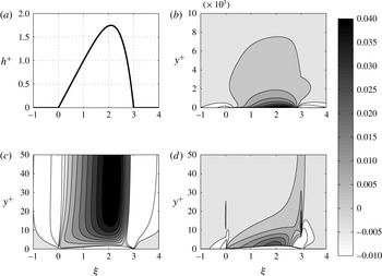
Velocity-field and shear-stress perturbations computed with (3.2)–(3.4) for boundary-layer thickness
 ${\it\delta}^{+}=10^{4}~(U_{\infty }^{+}=30.5)$
,
 $L^{+}=1000$
and a uniform coordinate shift by
 $h^{+}$
(
 $a=0$
in (3.1)). (a) Assumed oil-drop shape. (b) Streamwise velocity perturbation
 $u^{+}=U^{+}(y^{+})-U_{B}^{+}(y^{+})$
, with details in (c). (d) Scaled shear-stress perturbation
 $4[(\text{d}U^{+}/\text{d}y^{+})-(\text{d}U_{B}^{+}/\text{d}y^{+})]$
.

The mean unperturbed velocity profile is composed of an inner part, obtained by integrating (2.11), and an outer part provided by the wake function given as (A12) in Monkewitz, Chauhan & Nagib (Reference Monkewitz, Chauhan and Nagib2008). Similarly, the mixing length is composed of an inner part, given by
 $l_{m}^{+}={\it\kappa}{\it\eta}D({\it\eta})$
, and an outer part obtained from the mixing-length model (2.9). Furthermore, the oil drop is replaced by a stationary rigid wall at
 ${\it\eta}=0$
where the no-slip condition is applied, and appears as a (linearised) forcing term on the right-hand side of the RANS equations. The free-stream boundary conditions are
 $u,v,p\rightarrow 0$
. Fourier transform in
 ${\it\xi}$
and Chebyshev polynomials in the wall-normal direction are used, with collocation points placed according to a Gauss–Lobatto distribution (
 $z_{GL}\in [-1,\,1]$
) by means of the algebraic map
 ${\it\eta}=100(z_{GL}+1)/(1-z_{GL})$
. Equations (3.2)–(3.4) are then solved in the Fourier domain for an appropriately large number of wavenumbers,
 ${\it\alpha}$
, and transformed back to the physical domain.
An example of the resulting velocity-perturbation field is shown in figure 5 for
 $a=0$
and a typical oil-drop shape. The resulting streamwise velocity perturbation is of the order of
 $+4\,\%$
of
 $u_{{\it\tau}}^{\ast }$
just 20 viscous units above the highest point of the oil drop, while some deceleration is present in the neighbourhood of the drop leading and trailing edges. The pressure perturbation is not shown as it is, at leading order, independent of
 $y^{+}$
in the two lower layers and given by
 $P_{1}=-U_{1}$
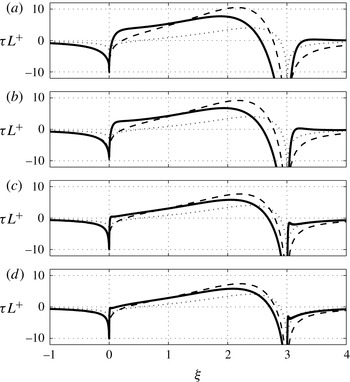
in both the main and upper layer. Figure 6 shows the comparison between the wall-shear-stress perturbation,
 ${\it\tau}$
, calculated from (2.57) of § 2 and the linearised numerical solution of (3.2)–(3.4), with
 $a=0$
to match the theory, for four values of
 $L^{+}$
and the oil-drop shape of figure 5(a). The wall-shear-stress perturbation predicted by the extended theory and by the numerics are seen to decrease roughly as
 $1/L^{+}$
and to converge, albeit rather slowly, with increasing
 $L^{+}$
. Note also the viscous stagnation points near the drop leading and trailing edges where the local velocity gradients may become sufficiently important to warrant a different local balance in the lower layer, i.e. the introduction of ‘fore-’ and ‘after-decks’. In short, the proposed theory probably underestimates the shear-stress perturbation at the drop leading edge, although the behaviour is qualitatively correct even at the lowest
 $L^{+}$
considered.
Scaled shear-stress perturbation for
 ${\it\delta}^{+}=10^{4}~(U_{\infty }^{+}=30.5)$
,
 $a=0$
and an oil drop with (a)
 $L^{+}=500$
, (b)
 $L^{+}=1000$
, (c)
 $L^{+}=5000$
and (d)
 $L^{+}=10\,000$
. ——, Linearised RANS result; leading-order
 $(\cdots \,)$
and second-order (- - - -) asymptotic theory (2.57).

At this point it is interesting to start changing the parameter
 $a$
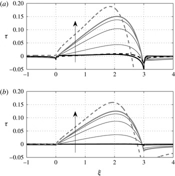
which governs the grid stretching and physically represents the degree of deformation of turbulence structures by the oil drop. Figure 7 shows that increasing the stretching parameter
 $a$
results in both a dramatic increase of the shear-stress perturbation and a change in the scaling of
 ${\it\tau}$
: while
 ${\it\tau}$
scales asymptotically as
 $(1/L^{+})$
according to the shifted theory (2.57), as demonstrated in figure 6, the
 ${\it\tau}$
values obtained from the RANS solution with
 $a>0$
in the coordinate shift (3.1), the unshifted RANS solution and the asymptotic result (2.59) without shift decrease much more slowly than
 $(1/L^{+})$
and are seen to approach the asymptotic decrease
 $\propto [\ln (L^{+}/U_{\infty }^{+})]^{-1}$
given by (2.59).
Comparison of the shear-stress perturbation in a ZPG TBL with
 ${\it\delta}^{+}=10^{4}~(U_{\infty }^{+}=30.5)$
for an oil drop with (a)
 $L^{+}=10^{3}$
and (b)
 $L^{+}=10^{4}$
. Thick black line, numerical RANS solution for
 $a=0$
; thin grey lines, numerical RANS solution for
 $a=0.05,\,0.2,\,0.5$
(
 $a$
increasing in the direction of the arrows); thick grey line, numerical solution of the unshifted RANS equations. Dashed lines, analytical results: (2.57) in black and (2.59) in grey.

(a)
 $u^{+}=U^{+}(y^{+})-U_{B}^{+}(y^{+})$
and (b)
 $4[(\text{d}U^{+}/\text{d}y^{+})-(\text{d}U_{B}^{+}/\text{d}y^{+})]$
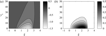
, analogous to figure 5(c,d) with the same drop shape and parameters, but without coordinate shift. Note that the streamwise velocity perturbation in (a) is negative because the no-slip condition at the oil–air interface has been linearised to
 $u^{+}(y^{+}=0)=-h^{+}$
.

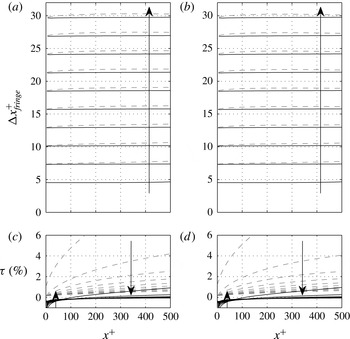
Evolution of fringe spacing according to (2.68) and (2.75) in time steps of
 ${\rm\Delta}t^{+}=3.08\times 10^{5}$
, with associated shear-stress perturbation
 ${\it\tau}$
provided by (2.57) (black lines) and (2.59) (grey dashed lines). The initial shape of the synthetic oil drop is given by (2.64) with
 $L^{+}=500$
and
 $L_{max}^{+}=3L^{+}$
: (a,c) with
 ${\it\delta}^{+}=10^{3}~(U_{\infty }^{+}=24.5)$
; (b,d) with
 ${\it\delta}^{+}=10^{4}~(U_{\infty }^{+}=30.5)$
. Other parameters:
 $u_{{\it\tau}}^{\ast }=0.68~\text{m}~\text{s}^{-1}$
,
 ${\it\nu}^{\ast }=1.5\times 10^{-5}~\text{m}^{2}~\text{s}^{-1}$
,
 $R_{{\it\mu}}=10^{-4}$
. The arrows indicate evolution with time.

Interestingly, the highest
 $a=0.5$
shown in figure 7 yields a
 ${\it\tau}$
approaching the numerical result obtained with the unshifted RANS equations, which is also reasonably close and converging towards the unshifted perturbation solution (2.59). The perturbation field computed without the shift is shown in figure 8 for the same conditions as in figure 5. Consistent with figure 7, the shear-stress perturbation in figure 8(b) is an order of magnitude larger than in figure 5(d). From these numerical experiments it appears that the unshifted asymptotic solution (2.59) is providing a useful upper bound for the shear-stress perturbation, despite violating the boundary condition for the Reynolds stress at the oil–air interface.
Figures 5–8 show that the two asymptotic theories, together with the RANS simulations, provide the range of the shear-stress perturbation incurred by neglecting the secondary boundary layer above the oil drop. All these figures have been established for a boundary-layer thickness of
 ${\it\delta}^{+}=10^{4}$
but, from the two limiting results ((2.57) and (2.59)), it follows that
 ${\it\tau}$
depends only very weakly on
 ${\it\delta}^{+}$
: for the shifted theory (2.57),
 ${\it\tau}\propto 1/L^{+}$
at leading order, while for the unshifted theory (2.59)
 ${\it\tau}\propto 1/\ln (L^{+}/U_{\infty }^{+})\sim 1/\ln (L^{+}/\ln {\it\delta}^{+})$
.
What remains to be shown is how these perturbations practically affect OFI measurements where the fringe spacing is spatially averaged. To clarify this question, two synthetic oil drops with an initial shape given by (2.64) with
 $L^{+}=500$
,
 $L_{max}^{+}=3L^{+}$
and a boundary-layer thickness of
 ${\it\delta}^{+}=10^{3}$
(close to the
 ${\it\delta}^{+}$
in the experiment described in § 4) and
 ${\it\delta}^{+}=10^{4}$
have been evolved according to (2.68) and (2.75) with
 ${\it\tau}$
provided either by (2.57) or (2.59). The other parameters of the simulations have been selected to match the experimental conditions in § 4. Figure 9 shows the resulting fringes as a function of space and time, together with the computed shear-stress perturbation for both theories. Consistent with the results shown in figure 7, the theoretical perturbations obtained with the shifted
 $y$
-coordinate are an order of magnitude smaller than the ones for the unshifted theory and very close to the case with
 ${\it\tau}=0$
. Note, however, that the difference between the theory (2.57) and
 ${\it\tau}=0$
is most pronounced near the drop leading edge where the local shear-stress perturbation is negative, corresponding to a viscous stagnation point. This is a manifestation of the streamwise pressure gradient which affects the result (2.57) at leading order, while it enters (2.59) only at higher order.
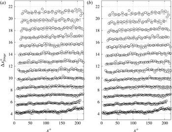
Example of observed fringe spacing (
 $\circ$
) versus distance
 $x^{+}$
measured from the drop leading edge at different times, in steps of
 ${\rm\Delta}t^{+}=1.45\times 10^{6}$
with initial
 $L^{+}=471$
and
 $L_{window}^{+}=220$
. ——, Corrected fringe spacing according to (2.75) with
 $\pm 1\,\%$
errors (- - - -). (a) Correction with shifted theory (2.57) resulting in
 $u_{{\it\tau}}^{\ast }=0.682~\text{m}~\text{s}^{-1}$
; (b) correction with unshifted theory (2.59) resulting in
 $u_{{\it\tau}}^{\ast }=0.675~\text{m}~\text{s}^{-1}$
. Other parameters:
 ${\it\nu}^{\ast }=1.589\times 10^{-5}~\text{m}^{2}~\text{s}^{-1}$
,
 ${\it\mu}^{\ast }=1.827\times 10^{-5}~\text{kg}\,\text{m}^{-1~}\text{s}^{-1}$
,
 $R_{{\it\mu}}=8.700\times 10^{-5}$
,
 $\mathit{Re}_{{\it\delta}_{\ast }}\approx 3500$
and
 $u_{{\it\tau}}^{\ast }=0.682\pm 0.003~\text{m}~\text{s}^{-1}$
without
 ${\it\tau}$
correction.

4. Laboratory experiments
A large number of nominally identical OFI measurements have been carried out at station ‘M2’ of the ‘S’-duct described in Bruns (Reference Bruns1998) and Bruns, Fernholz & Monkewitz (Reference Bruns, Fernholz and Monkewitz1999). This measuring station is located at
 $2.85~\text{m}$
from the boundary-layer trip where the turbulent boundary layer is still nearly two-dimensional. The duct geometry has been slightly corrected relative to the set-up of Bruns (Reference Bruns1998) to ensure a zero pressure gradient at the measuring station. All the experiments were carried out with a nominal free-stream velocity of
 $U_{\infty }^{\ast }=16.7~\text{m}~\text{s}^{-1}$
, monitored with a Pitot-static tube. Depending on which model is used for the shear-stress correction, the corresponding
 $U_{\infty }^{+}$
is in the range 24.6–24.9 corresponding to
 $\mathit{Re}_{{\it\delta}_{\ast }}=3600{-}4000$
when using the relation
 $U_{\infty }^{+}=0.384^{-1}\ln \mathit{Re}_{{\it\delta}_{\ast }}+3.30$
established by Monkewitz et al. (Reference Monkewitz, Chauhan and Nagib2007) for high Reynolds numbers.
A typical example of the fringe spacing obtained from an oil-film interferogram of good quality, i.e. without defects due to dust, is shown in figure 10. To obtain this graph, a single line is manually selected along the centreline of the oil-drop image. The corresponding intensity signal is then high-pass filtered to remove any slow variations due to non-uniform lighting, and the zero crossings of this filtered signal are identified with the fringe spacing
 ${\rm\Delta}x_{fringe}^{\ast }(x^{\ast },t^{\ast })$
at each time
 $t^{\ast }$
. The oil-film height
 $h^{\ast }(x^{\ast },t^{\ast })$
is then obtained by integrating (2.74). To obtain a smooth initial condition
 $H^{\ast }(x^{\ast })$
, needed in (2.68), a fifth-order polynomial is fitted to
 $h^{\ast }(x^{\ast },0)$
. Finally, the
 $L^{+}$
parameter is determined from the inverse slope of
 $H^{\ast }(x^{\ast })$
obtained from a least-squares linear fit of
 $H^{\ast }$
over the entire length of the interrogation window
 $L_{window}^{\ast }$
and the iterated estimate of
 ${\it\tau}_{w}^{\ast }$
.
Since there is no reference method to determine wall shear stress, the new corrections for
 ${\it\tau}$
are compared to the traditional analysis of Tanner & Blows (Reference Tanner and Blows1976), where the fringe spacing is assumed to be a function of time only. The spatial average
 $\overline{{\rm\Delta}x}_{fringe}^{~\ast }(t^{\ast })$
of
 ${\rm\Delta}x_{fringe}^{\ast }(x^{\ast },t^{\ast })$
over the interrogation window
 $L_{window}^{\ast }$
is computed independently at any given time by minimising the integral over
 $L_{window}^{\ast }$
of the squared distance between the measured intensity signal
 $s(x^{\ast })$
and the sinusoid
 $$\begin{eqnarray}S(\overline{{\rm\Delta}x}_{fringe}^{~\ast },\,A_{j})=A_{1}\sin \left(\frac{2{\rm\pi}x_{i}^{\ast }}{\overline{{\rm\Delta}x}_{fringe}^{~\ast }}\right)+A_{2}\cos \left(\frac{2{\rm\pi}x_{i}^{\ast }}{\overline{{\rm\Delta}x}_{fringe}^{~\ast }}\right)+A_{3},\end{eqnarray}$$
which respect to the arguments of
 $S$
. The corresponding wall shear stress is then obtained according to (1.2) from the time derivative of
 $\overline{{\rm\Delta}x}_{fringe}^{~\ast }$
. Further details on the experimental set-up and data processing are given in the appendices A and B. The standard uncertainty of the complete measurement chain (excluding the systematic correction discussed in the present work) has been quantified as 0.5 %.
It is evident in figure 10 that the measured
 ${\rm\Delta}x_{fringe}^{+}$
at any fixed time are not quite independent of
 $x^{+}$
, as assumed in the classic theory. Note also the transients at small times near the end of the domain, where excess oil is still being removed by the shear. The fringe spacing determined from (2.75) actually shows good quantitative agreement with the measurements, both near the leading edge and tail end of the interrogation window, for both the shifted and unshifted asymptotic
 ${\it\tau}$
corrections. Just by looking at the figure it is hardly possible to see a difference between the two shear-stress corrections (2.57) and (2.59), even though the corresponding friction velocities differ by 1 % (see caption of figure 10).
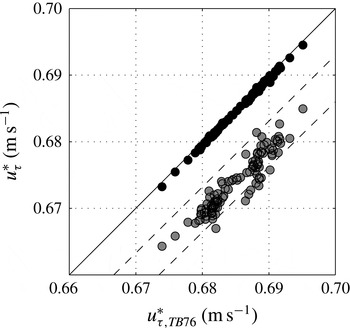
The difference between (2.57) and (2.59) is, however, clearly revealed by the wall shear stress extracted from 111 different runs at the same nominal conditions by means of (2.75) with the two different corrections for
 ${\it\tau}$
. This is shown in figure 11 as a scatter plot between the friction velocities according to the basic Tanner & Blows (Reference Tanner and Blows1976) theory with
 ${\it\tau}=0$
and with the two theoretical shear-stress corrections (2.57) and (2.59). For each run, the friction velocity has been determined by minimising the root-mean-square error of the difference between the measured fringe spacing and both theoretical predictions. The figure shows that, for our experimental conditions, which are similar to many other experiments, the estimate for the friction velocity is decreased by only 0.1 % for the shifted theory (2.57), while the reduction is 1.5 % for the unshifted solution (2.59). This range is believed to bracket the true overestimation of the wall shear stress relative to the value obtained with the standard Tanner & Blows (Reference Tanner and Blows1976) theory for infinitely thin oil films.
Comparison between the friction velocity
 $u_{{\it\tau},TB76}^{\ast }$
estimated with the Tanner & Blows (Reference Tanner and Blows1976) theory (
 ${\it\tau}=0$
) and the estimates based on the shear-stress correction (2.57) obtained with the shifted
 $y$
-coordinate (black circles) and the correction (2.59) without coordinate shift (grey circles). The solid line is the identity line while the two dashed lines correspond to an overestimation by 1 % and 2 %.

4.1. Assessment of the effect of spanwise drop surface curvature
Up to here, only the parts of interferograms on or near the line of symmetry of the oil drops have been considered. To justify this approach, the effect of the spanwise curvature of the drop surface has been assessed experimentally. For this,
 $u_{{\it\tau}}^{\ast }$
was determined from the fringes on the symmetry axis of a number of different size drops and of a two-dimensional drop, i.e. a transverse ‘oil strip’ of about 30 mm length, all made with the same oil of 200 cSt nominal viscosity, at the same temperature and subjected to the same air boundary layer. No trend of
 $u_{{\it\tau}}^{\ast }$
with initial drop size was detected in these measurements, meaning that if there is a trend it is buried in the small variance of the measurements.
The other question is how far off the centreline one can analyse the streamwise fringe spacing and still obtain an accurate value of
 $u_{{\it\tau}}^{\ast }$
, for instance when the centreline region is contaminated by dust particles. To answer this question, the shapes in the
 $x^{\ast }{-}z^{\ast }$
plane (with
 $z^{\ast }$
the transverse coordinate) of five different fringes have been extracted from interferograms of three oil drops with initial diameters of 2.8 mm, 4.6 mm and 7.43 mm, which covers the range of drop sizes used in most experiments. In addition, the corresponding fringes of the transverse ‘oil strip’ were recorded over a central width of 5 mm. For each of the three drops and for the 2D oil strip five fringes, numbers 2, 7, 12, 17 and 22 counted from the leading edge, are stacked on top of each other in figure 12. To facilitate the comparison and to show the similarity between drops of different diameter, both coordinates
 $x^{\ast }$
and
 $z^{\ast }$
are scaled with the initial drop diameter
 $d^{\ast }$
, except of course for the 2D oil strip. It is evident from figure 12 that in all cases the fringe shapes do not change, within experimental accuracy, with downstream distance. This means that the transverse curvature of the three drop surfaces does not change with downstream distance. In other words, any pressure increase within the drop due to surface tension is independent of downstream distance and hence does not affect the streamwise evolution of the drop. The two-dimensional theory developed in § 2 applies along any line of
 $z^{\ast }=\text{constant}$
as long as this line is not too close to the lateral boundaries, where drops develop a topology resembling glacier moraines (see figure 2). In conclusion, no trend of the measured wall shear stress with initial oil-drop diameter could be identified for drop sizes typically used in oil-film interferometry.
Superposition of fringes numbers 2, 7, 12, 17 and 22 from the leading edge at time
 $t^{+}\approx 1.8\times 10^{7}$
. From bottom to top: 2D oil strip (central 5 mm shown on the graph) and drops with initial diameters of
 $d^{\ast }=7.4,4.6$
and 2.8 mm. Each group of fringes is shifted up by
 $0.1d^{\ast }$
.

5. Conclusions
The basic two-dimensional similarity solution of Tanner & Blows (Reference Tanner and Blows1976) has been extended to a nearly wedge-shaped two-dimensional oil film of small but finite thickness (of the order of one viscous unit) by means of a perturbation expansion in terms of the oil-film slope
 $1/L^{+}$
which accounts for the perturbation of a ZPG TBL by the oil ‘hill’. The turbulence is accounted for by a mixing-length model, specially adapted to yield the correct Taylor expansion of the Reynolds stress at the bottom of the air layer. As it turns out, the shear-stress perturbation depends critically on how the mixing length is affected by the oil drop. Two cases have been considered which are argued to provide a lower and upper bound for the perturbation caused by the oil drop.
(i) The smallest wall-shear-stress perturbation due to the presence of the oil film, of
 $\mathit{O}(L^{+})^{-1}$
, has been obtained by uniformly shifting the mixing length up by the oil thickness. This corresponds physically to turbulent structures which are uniformly pushed up by the oil film with a minimal distortion. The analysis is similar to the analyses by Jackson & Hunt (Reference Jackson and Hunt1975) and Sykes (Reference Sykes1980) of atmospheric flow over low hills where the outer flow is driven by the ‘blowing’ velocity
 $U_{\infty }^{\ast }\,\text{d}h^{\ast }/\text{d}x^{\ast }$
due to the topography. The addition of the present analysis is the proper treatment of the region immediately above the oil film, which is essential to evaluate the shear-stress perturbation acting on the oil. For a typical application of the OFI technique, this shifted mixing-length model yields a correction of the friction velocity of
 $-0.1\,\%$
relative to the one determined with the original Tanner & Blows (Reference Tanner and Blows1976) theory for an infinitely thin, perfectly wedge-shaped oil film. Remember also that this variant of the theory is of the interactive triple-deck variety, i.e. involves the pressure perturbation at leading order, so that the shear-stress correction in the upstream wedge-shaped part of the oil film is influenced by the shape of its downstream part.
(ii) The largest wall-shear-stress perturbation, of
 $\mathit{O}[\ln (L^{+}/U_{\infty }^{+})]^{-1}$
, is obtained when the mixing length is not shifted at all so that the Reynolds stress is zero at the wall and not at the oil–air interface. This corresponds to turbulent structures which do not react to the presence of the oil film so that their distance to the oil–air interface is reduced by the oil-film thickness. The effect of this change on the present example is to significantly increase the friction velocity correction from
 $-0.1\,\%$
to
 $-1.5\,\%$
relative to the original Tanner & Blows (Reference Tanner and Blows1976) theory. However, in contrast to the shifted theory, the three layers in this unshifted analysis are non-interacting, meaning that the leading order is not affected by the pressure perturbation. As already noted, this perturbation analysis violates the Reynolds-stress boundary condition at the oil–air interface, but numerical experiments with a non-uniform shift, equal to the oil thickness at the oil–air interface and diminishing towards the free stream, demonstrate that the unshifted asymptotic result is close to the computed shear-stress perturbation for a shift which is attenuated within a few viscous units.
It is remarkable – and fortunate for the OFI application – that the shifted theory for the wall-shear-stress perturbation, where the tail end of the oil drop influences the evolution of its wedge-like front part, produces a shear-stress perturbation which is negligible in practice, while in the unshifted theory, which yields a substantial shear-stress perturbation, the upstream part of the oil film used for the shear-stress measurement remains essentially unaffected by the (uncontrollable) shape of the downstream part of the drop. It is also noted that the restriction of the oil-film thickness to
 $\mathit{O}(1)$
wall units for the theoretical developments does not limit the application of the new shear-stress corrections to low Reynolds numbers. For a fixed free-stream velocity of, say,
 $U_{\infty }^{\ast }=50~\text{m}~\text{s}^{-1}$
and Reynolds numbers
 $\mathit{Re}_{{\it\delta}_{\ast }}$
between
 $10^{4}$
and
 $10^{6}$
, the viscous unit in air varies between 8 and
 $12~{\rm\mu}\text{m}$
, while the vertical distance between consecutive fringes in a typical set-up is of the order of
 $0.2~{\rm\mu}\text{m}$
, (2.73), so that
 $\mathit{O}(50)$
fringes are available within
 $h^{+}\in [0,1]$
at the start of an OFI run.
At this point, a friction-velocity correction in the range of
 $-0.4\,\%$
to
 $-1\,\%$
relative to the original Tanner & Blows (Reference Tanner and Blows1976) theory appears most likely for typical oil films with inverse slope
 $L^{+}=\mathit{O}(10^{3})$
and maximum thickness
 $h_{max}^{+}=\mathit{O}(1)$
. (Note that the lower figure of
 $-0.4\,\%$
corresponds to the case
 $a=0.05$
on figure 7 where the mixing-length model is adapted to the presence of the oil film over the lowest 20 wall units.) Such an uncertainty about the true systematic correction for
 $u_{{\it\tau}}^{\ast }$
is generally beyond the accuracy desired in high-quality experiments. The present estimates are nevertheless useful as they provide an estimate of the maximum negative bias to be applied to OFI measurements of
 $u_{{\it\tau}}^{\ast }$
as a function of the drop geometry at the start of the measurement. For the experiments of § 4 with a standard statistical uncertainty of
 $\pm 0.5\,\%$
, for instance, the true
 $u_{{\it\tau}}^{\ast }$
is estimated to be between
 $-1.5\,\%$
and
 $+0.1\,\%$
of the measured value. Such a large total uncertainty is of course unsatisfactory, but a sharper estimate of the systematic error would require a model for the near-wall Reynolds stress with an unheard of accuracy of the order of 0.1 %, possibly including history effects due to the presence of the oil drop. A more realistic alternative to definitively nail down the systematic correction, as a function of the initial
 $L^{+}$
and
 $h_{max}^{+}$
, are high-resolution, high-precision direct numerical simulations. While waiting for such computations, one can nevertheless extract some practical guidelines from the present analysis.
-
(a) The correction for a non-planar initial oil surface, discussed in § 2.7, should always be implemented to account for the initial oil-drop curvature and its propagation in time.
-
(b) The first fringe(s) near the leading edge of the oil drop should not be used because of the pressure field associated with the viscous stagnation point (see e.g. figure 9).
-
(c) The oil film should be analysed as late as possible in its evolution, i.e. the film slope
$1/L^{+}$
should be as small as possible. This timing is of course limited by the requirement of still having a sufficient number (
${\gtrsim}10$
) of fringes to analyse. In addition, oil surface contamination is likely to influence the film evolution when it becomes very thin. -
(d) The new corrections developed in this paper for ZPG TBLs remain applicable in TBLs with a weak imposed pressure gradient. The evolution of oil height
$h(x,t)$
would then be affected additively not only by the shear-stress correction and the initial shape
$H(x)$
, but also by the effect of the imposed mean pressure gradient in (2.6) already considered by Tanner & Blows (Reference Tanner and Blows1976), as long as the difference between
$h$
with and without pressure gradient can be treated as a small correction.


Acknowledgements
The authors would like to thank N. Tillmark for the fruitful discussions and H. Nagib and H. Alfredsson for encouraging this study. A.S. and J.-D.R. are grateful to the CICLoPE project at the University of Bologna for their financial support. A.S. is also grateful for the financial support by the Swedish strategic research program STandUP for Wind.
Appendix A. Experimental set-up
The flow facility is described in Bruns (Reference Bruns1998) and Bruns et al. (Reference Bruns, Fernholz and Monkewitz1999). All the measurements presented here have been carried out at station ‘M2’ of the ‘S’-duct located at
 $2.85~\text{m}$
from the boundary-layer trip where the turbulent boundary layer is still two-dimensional and unaffected by pressure gradients. The duct geometry has been slightly corrected relative to the set-up of Bruns (Reference Bruns1998) to ensure a zero pressure gradient at the measuring station. The nominal free-stream velocity of
 $U_{\infty }^{\ast }=16.7~\text{m}~\text{s}^{-1}$
was monitored with a Pitot-static tube connected to a MKS Baratron pressure transducer. The temperatures of the air in the wind tunnel and of the boundary-layer plate surface, where the oil drop was deposited, were monitored with two thermocouples, connected to a FLUKE handheld device. The same thermometer was used to monitor the temperature during the oil-viscosity calibration, allowing a repeatability of the temperature measurements of
 $\pm 0.2\,^{\circ }\text{C}$
for the determination of the oil viscosity. As the wall shear stress is directly proportional to the oil viscosity, it is crucial to perform an independent calibration with a better accuracy than the one desired for
 ${\it\tau}_{w}^{\ast }$
. For the present experiments the silicone oil 200DC from Dow Corning with a nominal viscosity of 200 cSt was used. The oil calibration was performed with a Schott capillary viscometer in which the transit times were recorded automatically by two light barriers. It was placed in a thermally controlled bath and measurements were repeated 10 times at different temperatures within a range of
 $10\,^{\circ }\text{C}$
. After eliminating outliers and series exhibiting a temporal drift, the data points were least-square fitted with an exponential relationship of the form
 ${\it\nu}_{oil}^{\ast }=a_{1}^{\ast }\exp (a_{2}^{\ast }T^{\ast })$
, where
 $T^{\ast }$
is the temperature and
 $a_{1}^{\ast }$
and
 $a_{2}^{\ast }$
are fitting parameters. The density of the oil was
 ${\it\rho}_{oil}^{\ast }=966.5~\text{kg}~\text{m}^{-3}$
with a refractive index of
 $n_{oil}=1.403$
.
A 12 Mpx Nikon D300 DSLR camera with a Sigma APO 180 mm F3.5 Macro-lens plus a Nikon Teleconverter TC-200 was used to record interferograms. The camera was mounted on a tripod on the ceiling of the wind tunnel and pointed down through a flush-mounted glass window in the boundary-layer plate mounted on the ceiling of the test section. The viewing angle was
 $15^{\circ }$
with respect to the flat plate normal in the downstream direction and was measured with an electronic level providing an accuracy of
 $\pm 0.2^{\circ }$
. The window in the boundary-layer plate on which oil drops were deposited was made of 6 mm thick BK7 optical glass with a surface flatness of
 ${\it\lambda}^{\ast }/10$
and a refractive index of
 $n_{glass}=1.513$
at 589.3 nm. Its illumination with monochromatic light of
 ${\it\lambda}^{\ast }=589.3~\text{nm}$
was provided by a 35 W low-pressure sodium lamp. This optical set-up provided a field of view of 10 mm in the streamwise and 16 mm in the cross-stream direction corresponding to
 $2848~\text{pixel}\times 4288~\text{pixel}$
on the CCD. The images were recorded in high-quality colour Jpeg format and transferred directly to a computer. The timing between the pictures was controlled by an external timer for time lapse photography which ensured a triggering accuracy of the order of
 $1/100~\text{s}$
over the entire duration of an experimental run.
Appendix B. Data acquisition and processing
For each measurement run, a calibration image with a millimetre grid glued onto a replica of the glass plug was recorded to determine the calibration factor over the extent of the oil drop. The image of the millimetre grid was magnified to pixel resolution to manually select the reference marks along a line passing through the symmetry axis of the oil drop. Due to the angle of
 $15^{\circ }$
between the plane of the window and the CCD sensor, the calibration factor is a linear function of the distance from the centre of the image, with an additional correction for the refraction angle at the glass surface. From geometry the linear deviation from the constant calibration factor is expected to be of the order of 0.1 % for the current set-up, while the refraction correction is even smaller. As the standard deviation of the calibration points from the linear fit (corresponding to a constant calibration factor) over 2848 pixels was about
 $\pm 2~\text{pixels}$
, the linear correction to the constant calibration factor was buried in the noise and therefore neglected. Hence a constant calibration factor of close to
 $280~\text{px}~\text{mm}^{-1}$
has been determined from the calibration images with a repeatability of 0.2 %. Finally, the slight change of view angle
 ${\it\varphi}$
(see figure 1) away from the image centre also has an influence on the determination of the film height but this effect modifies the fringe spacing only by about 0.05 % at the edge of the interferogram and is therefore also neglected. Additional measurements of 103 oil drops, with nominally the same operating conditions but with a larger field of view and a calibration constant of
 $140~\text{px}~\text{mm}^{-1}$
, have been used in order to provide statistical support to the analysis.
After calibration, the glass surface was prepared and the oil drop deposited with great care. The glass surface was cleaned with 95 % alcohol, and dried with a clean particle-free cloth to remove any dust particles and alcohol deposits. The silicone oil drop was then deposited with a needle on the glass surface outside the wind tunnel and the plug was only then installed in the wind tunnel, flush with the boundary-layer plate. This procedure did not require shutting down the wind tunnel, which avoided thermal transients. After installing the plug with the oil drop, images were recorded at constant time intervals of 10 s during 15 min. The images were then cropped to the zone of the oil drop, transformed to grey scale and turned into an image stack in Matlab.