3.1. Velocity and temperature/density fields

Time series snapshots of internal wave propagation through the computational domain are shown in figure 2. Three simulation cases are shown in this figure for $Fr=0.1$, $Fr=0.5$ and $Fr=0.84$, depicting linear, nonlinear and highly nonlinear cases, respectively. Values for the relative slope $\gamma /s=1$ (i.e. critical slope) and topography-to- depth ratio $h_t/d = 0.5$ are consistent for the simulations depicted. Also, for all three simulations, the frequency of the incoming internal wave is $\omega =0.0035\ {\rm rad}\ {\rm s}^{-1}$ and the wave period $T=2{\rm \pi} /\omega =1800$ s. Forcing of the internal wave is modified by imposing varied velocity amplitude $U_0$ at the inlet of the domain. Each of the three cases in figure 2 shows six snapshots of the internal wave developing and propagating over the topographic ridge. The time instants are normalized by $T$. The domain depicted starts at $x=50$ m, ends at the computational domain outlet $x=150$ m and is coloured by the stratification, depicted using the temperature anomaly.

Figure 2.

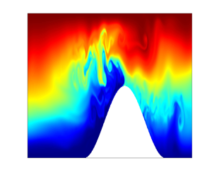
Time series snapshots of an internal wave building and passing over the topographic ridge. Colour spectrum denotes the temperature anomaly of the simulations. The relevant parameters for the simulations depicted are $\gamma /s=1$, $h_t/d=0.5$ for (a) $Fr=0.1$, (b) $Fr=0.5$ and (c) $Fr=0.84$. As the Froude number increases the dynamics of the internal waves’ interaction with the topographic ridge becomes more complex with more overturning and transport of high density fluid from near the bottom boundary up and over the ridge when $Fr=0.84$. Note that the first $50$ m of the domain is truncated in the figures to better visualize flow structures near the ridge.

With $Fr=0.1$ the six panels in figure 2(a) show the propagation of an internal wave forced by $U_0=0.3\ {\rm cm}\ {\rm s}^{-1}$. The dynamics of this simulation is dominated by linear oscillations of the flow field as the internal wave propagates to the ridge. Some minimal magnitude displacement is visible in the flow field on the upstream side of the ridge as well as above the peak in topography. While some dissipation and mixing occurs due to the criticality of the topography, a greater portion of the energy is either transmitted past the topography or reflected off the topography. Most of the small-scale features visible in this series of visualizations are a result of the slope criticality leading to the decoupling of the internal wave beams. In the simulations with $Fr=0.1$ and sub- or supercritical slopes, these features are lesser in extent. As the Froude number increases these features also become less observable as the beam decoupling gets overwhelmed by the energy and the resulting nonlinear dynamics.

Figure 2(b) shows a simulation with $Fr=0.5$ set by $U_0=1.5\ {\rm cm}\ {\rm s}^{-1}$. The presence of nonlinear dynamics is visible in the snapshots of this simulation with dense fluid from the base of the stratified water column propagating up and over the ridge (see panels (iv) and (v)). These flow structures have been both simulated (Venayagamoorthy & Fringer Reference Venayagamoorthy and Fringer2006, Reference Venayagamoorthy and Fringer2007) as well as observed (Cacchione & Wunsch Reference Cacchione and Wunsch1974) and are known as tidal bores, or solibores. These flow structures are formed as a result of the internal wave creating a vortex core that advects dense fluid from low in the water column up onto a continental shelf (as shown in VF06 for example) or over the top of ridge (as shown here). In addition to the advection of dense fluid by bores, larger magnitude displacements of fluid are visible relative to the case with $Fr=0.1$. Displacements of fluid, both on the upstream side of the ridge as well as above the topographic peak, increase in magnitude. The drawdown of fluid on the upstream side of the ridge as the internal wave advects toward the ridge, as well as the propagation of the bore to the downstream side of the ridge, creates regions of unstable stratification where denser fluid overlies less dense fluid. Visible in the snapshots are the overturning structures that result from unstable stratification and the advection of the bolus.

A velocity amplitude of forcing $U_0=2.5\ {\rm cm}\ {\rm s}^{-1}$ sets a simulation with $Fr=0.84$, depicted in figure 2(c). It is clear from the series of snapshots that the dynamics becomes highly nonlinear with significant instability with the increase in energy. Fluid displacements, the size of the bore transporting mass over the ridge as well as the size of the overturns resulting from unstable stratification are all of greater magnitude when compared with the other two cases. In the case shown in figure 2(b) the bore is ejected off the ridge, creating an overturn and mixing. In this case, the size/mass of the bore is sufficiently large that it returns down the backside of the ridge. This downslope advection of the bore (as shown in figure 2c-v) generates an overturning structure that is in the opposite direction to the ejected bore depicted in figure 2(b-v). This final time series clearly shows the complex dynamics that results from highly nonlinear internal waves interacting with topography in a stratified flow.

Figure 3 shows the normalized zonal velocity $u$, normalized vertical velocity $w$ and normalized density profiles for the same three cases discussed for figure 2 at $t/T=6.25$. Figure 3(a) shows profiles for $Fr=0.1$, figure 3(b) for $Fr=0.5$ and figure 3(c) for $Fr=0.84$. Each row of normalized plots correspond to transects I-III as depicted in figure 1, respectively. The zonal velocity, vertical velocity and density profiles at profile § 1 in the first row for each of the cases show a similar distribution as expected but normalization of the velocities by $U_0$ results in varied magnitudes due to the differences in the velocity amplitude of forcing.

Figure 3.

Normalized zonal velocity ($u$), vertical velocity ($w$) and density ($\rho$) profiles for $t/T=6.25$. Grouping (a) is for simulation where $Fr=0.1$, grouping (b) $Fr=0.5$ and (c) $Fr=0.84$. The other relevant parameters are $\gamma /s=1$ and $h_t/d=0.5$ for all three simulations. Within each grouping row 1 denotes the profile from transect I, row 2 the profile from transect II and row 3 from transect III on the downstream side of the topographic ridge as depicted in the schematic shown in figure 1.

For the linear lowest energy case ($Fr=0.1$) the profiles at transect II show a zonal velocity distribution with increased values near the bed as the wave approaches the ridge. The vertical velocity magnitude at transect II has also increased, as would be expected with the zonal flow being redirected vertically over the ridge. The density profile steepens near the bed, likely due to the energy of the internal wave pushing the dense fluid near the bottom against the base of the ridge and creating a slight increase in the density near the bottom of the profile. Row 3 of panel (a) shows the distributions of transect III, the downstream side of the ridge. Both the zonal and vertical velocity magnitudes have decreased. On the lee side of the ridge the zonal velocity should decrease as it is sheltered from the incoming internal wave and the vertical velocity switches direction as some of the flow moves down the back side of the ridge.

Figure 3(b) shows the normalized velocity and density profiles at transects I, II & III for simulation with $Fr=0.5$ at $t/T=6.25$. At transect II the normalized zonal velocity shows a velocity distribution representative of the drawdown on the upstream side of the slope just before the arrival of an internal wave. This distribution is corroborated by the corresponding image from figure 2(b-vi) showing the fluid being drawn downslope during the simulation at this instant, resulting in the negative vertical velocity. The density profile also shows the impact of the drawdown of lighter fluid from higher in the stratified fluid column.

In figure 3(c) similar trends are observable for the simulation defined by $Fr=0.84$ at $t/T=6.25$. The increased velocity of this simulation results in a zonal velocity distribution that is already propagating up the ridge at transect II. It had not yet arrived at the ridge in the previous case, resulting in the drawdown profile discussed above. The density profiles from transects II and III show the result of the increase in energy of this simulation with more varied distributions of density due to turbulence and mixing. Regions of unstable stratification are also observed in the density profile at transect II. The flow structures visible in all three of the simulation time series shown in figure 2 are signatures of nonlinear as well as non-hydrostatic effects. These nonlinear structures are sufficiently resolved in the current simulations to be visible within the flow, similar to those seen in highly resolved simulations such as in VF06.

3.2. Energy flux and partition

Here, we repeat a concise portion of the derivation for the depth-integrated energy flux presented in VF06 and Venayagamoorthy & Fringer (Reference Venayagamoorthy and Fringer2005) but it will be applied here to a topographic ridge rather than a shelf. This analysis is also similar to the derivation presented in Rapaka et al. (Reference Rapaka, Gayen and Sarkar2013) for the energy flux components and the determination of relative energy transmission, reflection and dissipation. Taking the dot product of (2.1) with $\boldsymbol {u}$ and adding the resulting equation to the product of (2.3) and $gz$ gives the governing energetics equation

(3.1)\begin{equation} \frac{\partial}{\partial t}(\rho_0 q+\rho gz)+\boldsymbol{\nabla}\boldsymbol{\cdot}\boldsymbol{f}={-}\rho_0\boldsymbol{\epsilon}_k -2\kappa\frac{\partial}{\partial z}(\rho g), \end{equation}

where $q=\boldsymbol {u}\boldsymbol {\cdot }\boldsymbol {u}/2$ is the kinetic energy per unit mass, $\boldsymbol {\epsilon }_k=\nu (({\partial u_i}/{\partial x_j})({\partial u_j}/{\partial x_i}))$ is the viscous dissipation rate of kinetic energy and the local energy flux is given by

(3.2)\begin{equation} \boldsymbol{f}=\boldsymbol{u}(\rho_0 q +p+\rho g z)-\mu\boldsymbol{\nabla} q-\kappa(\rho gz), \end{equation}

with $\mu$ denoting the dynamic viscosity. From the equations derived above it follows that the depth-integrated energy flux (units of ${\rm W}\ {\rm m}^{-1}$) is given by

(3.3)\begin{equation} F_E=\int_{{-}d}^0\left[u(\rho_0q+\rho gz+p)-\mu\frac{\partial q}{\partial x}-\kappa\frac{\partial}{\partial x}(\rho gz)\right]{\rm d} z. \end{equation}

Assuming that at $t=0$ the density field is given by the imposed background density field $\rho _b$ and that the contribution of the diffusive terms to the energy flux is negligible, the change in total energy can be computed using the simplified depth-integrated energy flux

(3.4)\begin{equation} F_E=\int_{{-}d}^0 p^\prime u\, {\rm d} z,\end{equation}

where $p^\prime =\rho _0q+\rho gz+p$. The time-integrated energy flux (units of ${\rm J}\ {\rm m}^{-1}$) is given by

(3.5)\begin{equation} E_\tau=\int_0^t F_E(\tau)\, {\rm d} \tau.\end{equation}

The pressure term $p$ in (3.3) can be split into two terms denoting its hydrostatic ($p_H$) and non-hydrostatic ($p_{NH}$) components gives $p^\prime =\rho _0q+\rho gz+p_H+p_{NH}$. If the total density is defined by $\rho =\rho _0+\rho _b+\rho ^\prime$, (3.3) can be written to account for the energy flux due to the work done by the hydrostatic pressure fluctuations $(i)$, the work done by the non-hydrostatic pressure $(ii)$, the advection of kinetic energy $(iii)$, the advection of potential energy due to density fluctuations $(iv)$, advection of potential energy due to the mean background density field $(v)$ and work done by the hydrostatic pressure due to the mean background density field $(vi)$. This derivation is analysed in detail, including a discussion of each contributing term, in Venayagamoorthy & Fringer (Reference Venayagamoorthy and Fringer2005), Kang & Fringer (Reference Kang and Fringer2010) and Kang & Fringer (Reference Kang and Fringer2012). Each of the energy flux contributions listed above can be determined from the numerical simulation data that are included explicitly as part of the simulation. The analysis presented in Kang & Fringer (Reference Kang and Fringer2012) (among others) shows that terms $(iv)\unicode{x2013}(vi)$ minimally contribute to the overall energy flux and these findings were corroborated in our analysis. The results of VF06 show that over 50 % of the energy flux results from the hydrostatic pressure anomaly while approximately 30 % of the energy flux is contributed by the non-hydrostatic pressure term, the two largest contributors to the energy flux budget in their analysis. Figure 4 shows both the depth-integrated flux (solid blue lines) as well as the cumulative energy flux (dashed magenta lines) for each of the three largest flux contribution terms $(i)\unicode{x2013}(iii)$ for simulations where $Fr=0.1$, $Fr=0.5$ and $Fr=0.84$ with $\gamma /s=1$ and $h_t/d=0.5$ in all three simulations. For the higher $Fr$ simulations shown in figure 4, the hydrostatic pressure anomaly term accounts for approximately 50 % of the energy flux and the non-hydrostatic pressure term approximately 35 %–40 % of the total energy flux. Each energy flux term plotted in figure 4 is normalized using a base estimate of the energy flux of the incoming internal wave computed using linear wave theory (Kundu et al. Reference Kundu, Cohen and Dowling2008)

(3.6)\begin{equation} F_L=\frac{\rho_0\omega U_0^2}{2k}d,\end{equation}

where $\rho _0$ is the reference density, $\omega$ is the forcing frequency, $U_0$ is the velocity amplitude of forcing, $d$ is the full flow depth and $k$ is the horizontal wavenumber obtained from the dispersion relation for internal waves. This energy flux is the integral of the product of the velocity and pressure perturbations. The evident contribution of the non-hydrostatic pressure work term shows the impact of vertical inertia and the instantaneous importance of the non-hydrostatic pressure. This figure shows that, as the Froude number increases, both the hydrostatic and non-hydrostatic energy fluxes increase. This result corroborates the laboratory-scale results of VF06 and illustrates the importance of the non-hydrostatic dynamics in stratified flows and internal wave CFD simulation.

Figure 4.

Depth-integrated energy flux normalized by $F_L$ (blue solid line) and time-integrated (cumulative) energy flux normalized by $F_L/\omega$ (magenta dashed line) as a function of $t/T$ at $x=105$ m for simulations with $Fr=0.1$ (a), $Fr=0.5$ (b) and $Fr=0.84$ (c). These are the same simulations as presented in figure 2, with $\gamma /s=1$ and $h_t/d=0.5$ consistent between simulations. The calculations are as in transect III on the downstream side of the ridge as denoted in figure 1.

Using the notation presented by VF06, the energy budget can be approximated by

(3.7)\begin{equation} E_I=E_R+E_T+E_D,\end{equation}

where $E_I$ is the total incident wave energy of the incoming wave, $E_R$ is the energy reflected back toward the inlet of the computational domain from the topography, $E_T$ is the energy transmitted past the topography and $E_D$ is the energy dissipated in the control volume bounding the topography. Figure 5 shows a schematic depiction of the components of the energy flux budget with the control volume centred over the topography between the dashed lines denoting transects II and III as show in figure 5. The reflected energy flux is determined by taking the difference in the total incident wave energy flux of transect II (see figure 5(a)) of the simulation with no topography present, $(E_\tau )_{nt,II}$, and the total wave energy flux that now includes both incident and reflected wave energies at transect II (see figure 5(b)) in the simulation with the topographic ridge being evaluated, $(E_\tau )_{wt,II}$. Dissipation of energy is determined from (3.7) by taking the difference between the cumulative total wave energy flux of transect II and the cumulative energy flux of transect III.

Figure 5.

Depiction of the energy budget for the control volume centred over the topographic ridge between vertical transects II and III. Panel (a) shows the base case where no topography is present ($\gamma /s=0$) and panel (b) shows the typical topographic ridge case ($\gamma /s>0$). Schematic (c) shows how the fluxes are determined from panels (a) and (b) to close the energy budget and determine the reflected and dissipated energy. Subscript ‘$nt$’ denotes the no-topography case and ‘$wt$’ denotes the case with a topographic ridge (modified from Venayagamoorthy & Fringer (Reference Venayagamoorthy and Fringer2006), not to scale).

Analysis of how the energy is partitioned between these three components across a wide range of pertinent parameters (i.e. $Fr$, $\gamma /s$ and $h_t/d$) will be insightful for understanding the dynamics of the interaction process and is carried out next.

Figure 6 shows the cumulative transmitted, reflected and dissipated energy fluxes for each simulation as a function of $\gamma /s$, for $h_t/d= 0.25$, 0.5 and 0.75, respectively. All the fluxes are normalized by the cumulative incident energy $E_I$. When the ridge height is only one quarter of the total flow depth, $h_t/d=0.25$ (figure 6a,d,g), the majority of the incident wave energy (approximately 70$\,\%$) is transmitted through the domain at the critical slope and reduces monotonically to approximately 50$\,\%$ for $\gamma /s = 1.5$. The amount of energy reflected is very small for the critical slope cases (regardless of $Fr$) but increases slightly when the slope becomes supercritical, offsetting some of the reduction in transmitted energy. The dissipation accounts for the remainder of the incident energy that is not transmitted at critical slopes and slightly increases for supercritical slopes especially for $Fr = 0.84$.

Figure 6.

Normalized cumulative energy fluxes for all simulation runs as a function of the topographic steepness parameter. Rows denote the normalized transmitted energy flux, normalized reflected energy flux and normalized dissipated energy flux, respectively. Columns group the results by the topography height–total depth ratio, $h_t/d$.

The second column of figure 6 shows the results for a ridge height $h_t/d=0.5$. Subcritical slope simulations allow for the majority of the energy to transmit up and over the topography but some energy is dissipated by turbulence in the flows with higher Froude numbers. The transmitted energy decreases in a monotonic manner as $\gamma /s$ increases regardless of $Fr$, similar to the trend seen in VF06. Amounts of reflected energy are very small, as would be expected as the internal wave beams forward reflect when the slope is subcritical. For critical slopes approximately half of the energy is transmitted. The amount of reflected energy remains the least significant of the three energy modes analysed in the cases with critical slopes. However, for supercritical slopes, reflection increases significantly, reaching almost 40 % at $\gamma /s = 1.5$. Both the proportions of transmitted and reflected energy are always higher for the lower $Fr$ cases for all $\gamma /s$ values, a result also seen in VF06. Dissipation magnitude varies as a function of Froude number, with dissipation accounting for approximately 50 % of the energy difference at high Froude numbers at critical slopes to less than 25 % for the lowest Froude number simulation, $Fr=0.1$ for subcritical slopes.

As the height of the ridge increases the amount of transmitted energy also decreases, as shown in figure 6(c). Approximately 25 % of the energy is transmitted for a ridge defined by a critical slope and the majority of the energy is reflected. For the least energetic simulations defined by $Fr=0.1$ the amount of energy transmitted through the domain is very low, with over 70 % of the energy being reflected off the topography and the majority of the difference being dissipated. Amounts of reflected energy vary significantly with $Fr$, with total reflected energy decreasing as Froude number increases. Flows defined by a larger Froude number lead to a more nonlinear dynamics and more of the energy being captured by dissipation and mixing. The plots in figure 6 show how the partition of energy flux is strongly dependent on all three non-dimensional parameters $Fr$, $h_t/d$ and $\gamma /s$.

On average 43 % more of the total wave energy is transmitted through the domain when $h_t/d=0.25$ than when $h_t/d=0.75$. The amount of the total wave energy that is reflected for these two cases is almost inversely proportional, with 36 % more energy being reflected on average for the simulations with $h_t/d=0.75$ when compared with the amount of energy reflected from simulations with $h_t/d=0.25$. The amount of energy dissipated is 16 % higher on average for $h_t/d=0.75$ than $h_t/d=0.25$, which can be attributed to the increased length of the wave-to-bed interaction that results from the increasing height of the topography. Results with $h_t/d=0.5$ necessarily fall in the middle of the range in terms of wave energy transmission, reflection and dissipation. Results from this subset of simulations with $h_t/d=0.5$ clearly illustrate the influence of $\gamma /s$. There is an average decrease of 40 % of the total wave energy transmitted as $\gamma /s$ increases (i.e. from subcritical to supercritical slopes). Results show that, for $h_t/d=0.5$, there is an average 31 % increase in the amount of total wave energy reflected with increasing $\gamma /s$. Total wave energy dissipated increases by 16 % with increasing slope steepness and the amount of wave energy levels off at approximately 50 % after reaching a critical slope.

If the results presented in figure 6 are directly compared with the results in VF06 there are a few notable differences. The two results are not directly comparable due to the different simulation scales, a shelf being used in VF06 as compared with a topographic ridge here and the different parameter value ranges explored ($Fr$, wave parameters etc.). In particular, it should be noted that, in VF06, the topographic steepness and topographic height were not independently varied, making a direct comparison difficult. Nonetheless, comparisons between the two studies taken on an average basis show decreases in transmission of $4\,\%$. This decrease in transmission can be partially explained as a result of the longer overall bottom length travelled by the internal wave while going over the topographic ridge as opposed to travelling along the shelf. Additionally, the potential energy contained by bolus mass cores at the top of the ridge is converted to kinetic energy as the bolus is ejected and plunges off the top of the ridge. A significant component of this kinetic energy that is not present in the shelf case in VF06 is in the vertical direction, contributing to additional mixing. There is an increase in the average reflection of 5 % and a decrease in the dissipation by 2 %. Increases in reflection are a result of the some of the resulting re-circulations observed in these simulations that move fluid mass back past the upstream toe of the ridge. The dissipation makes up the necessary difference.

Data presented in figure 7 depict a subset of the overall data presented in figure 6 at the critical slope ratio, $\gamma /s=1$. The proportions of transmitted, reflected and dissipated amounts of energy are presented on the horizontal axis and the ridge height-to-depth ratio on the vertical axis in order to maintain this quantity's physically realistic orientation. Each data point is coloured by $Fr$ of the simulation. Figure 7(a) shows that the transmitted energy flux decreases linearly with $h_t/d$ at the critical slope. As nicely discussed in L14, in the near-critical slope regime, it can be shown that, for a finite-length critical slope with a piecewise constant slope (e.g. a triangular ridge), the fraction of energy flux that will be transmitted scales linearly with $(1-h_t/d)$. The agreement, as shown by the dashed line in figure 6(a), with the simulation results is remarkable despite the differences in shape of the topography and variations in $Fr$. This finding is also corroborated in the field-scale simulations of L14, where a similar monotonic decline in transmitted energy with $h_t/d$ is seen at critical slopes. However, there are some changes with $Fr$ that are worth noting. At $h_t/d = 0.25$, the effect of $Fr$ is small with slightly less transmission at higher $Fr$. At $h_t/d = 0.5$, the effect of $Fr$ increases in a non-monotonic manner with the peak transmission ratio of approximately 0.5 at an intermediate $Fr=0.25$. Such a non-monotonic trend in the transmission ratio with $Fr$ for a critical slope was also found in VF06, wherein they report a value of approximately $Fr = 0.34$ at peak transmission. Figure 7(b) shows that the proportion of reflected energy increases with ridge height in a highly nonlinear manner. The increase in reflected energy is only slight (approximately 10 %) between the cases with $h_t/d =$ 0.25 and 0.5. On the other hand, the increase is drastic when $h_t/d$ changes from 0.5 to 0.75. Given the linear trend in the transmitted energy, it is clear that dissipation is significant at $h_t/d = 0.5$. Figure 7(c) shows that the dissipation exhibits a non-monotonic behaviour with a peak at the intermediate ridge height for critical slopes. Even though there is a longer surface for the wave to traverse in the cases of the taller ridges, this result is likely a result of the scale of incoming wave energy and the scale of the topographic ‘obstacle’, where the amount of energy dissipated decreases for the taller ridge. This finding has important implications for optimal mixing ‘hotspots’ in the ocean.

Figure 7.

Energy transmission, reflection and dissipation for the three ridge heights at $\gamma /s=1$. Energy transmission increases as the ridge height decreases, panel (a), energy reflection increases with increases in ridge height, panel (b), and energy dissipation peaks for the intermediate ridge height, panel (c). The linear trend line in panel (a) directly follows from linear theory, as presented in L14, of $E_T/E_{total}=1-h_t/d$.

The simulation snapshots presented in figure 8 qualitatively depict this interaction between the wave and topography. The first row of panels, (a–c), depicts the same time snapshot of the simulations for $Fr=0.5$ and $\gamma /s=1$ at all three ridge heights. For the smallest ridge depicted in figure 8(a) there is clearly some nonlinear fluid dynamics, as shown by some overturning structures with denser fluid moving up over the ridge. In figure 8(b) the bolus core of fluid ejected over the ridge is larger, but it is also clear that there is an increase in the nonlinear dynamics with more visible mixing between the layers of fluid. In the case of the tallest ridge, the scale of the incoming wave does not match the scale of the topography so the bolus size decreases and the densest fluid is not able to go over the top of the ridge.

Figure 8.

Panels (a–c) show a snapshot of internal wave interaction with topography for the three ridge heights all at $Fr=0.5$ and $\gamma /s=1$. Panels (e–f) show internal wave interaction with $h_t/d=0.5$ and $h_t/d=0.75$, respectively, for $Fr=0.84$, $\gamma /s=1$. Panel (d) presents the energy transmission trends with respect to $\gamma /s$, $h_t/d$ and $Fr$, where there is a clear, nearly linear trend in the decrease of transmitted energy as ridge height increases. For $h_t/d=0.25$ and $h_t/d=0.5$ the amount of energy transmitted decreases as the Froude number increases due to an increase in dissipation but it is worth noting the reverse $Fr$ trend for simulations with $h_t/d=0.75$ as more energy is needed to overtop the ridge.

If the simulation Froude number is increased to $0.84$ this same result holds. At the intermediate ridge height, the bolus structures increase in size from the $Fr=0.5$ case with the same ridge height, as can be seen in figure 8(e). For the tallest ridge (see figure 8f), there is also an increase in the bolus size and the amount of mass ejected over the ridge when compared with the same ridge height at $Fr=0.5$. However, when compared with the intermediate ridge height case at $Fr=0.84$ (figure 8e), there remains insufficient wave energy to move the densest fluid over the ridge. Figure 8(d) gives a similar presentation of the data as figure 7(a) for the transmission of wave energy but for all $\gamma /s$ values and ridge heights. Data are still coloured by simulation Froude number. Similar to the relationship between $E_T/E_{total}$ and $h_t/d$, the relationship between $\gamma /s$ and $E_T/E_{total}$ follows a linear relationship for all of the data. The trends in the transmitted energy are different with respect to $Fr$ and $h_t/d$. For $h_t/d=0.25$ and $h_t/d=0.5$ the amount of energy transmitted decreases with increasing $Fr$. This energy is being absorbed in the energy dissipation for each constant ridge height across all $\gamma /s$. For $h_t/d=0.75$ a similar linearly proportional relationship between $\gamma /s$ and $E_T/E_{total}$ as the other two ridge heights occurs, but the amount of energy transmitted as a function of $Fr$ has the opposite trend, as shown in figure 8(d). For the taller ridges, increase in $Fr$ provides more wave energy to transmit energy over the tallest ridges and in balance appears to have the impact of reducing the amount of energy dissipated, as shown in figure 6(i).

Figure 9 shows both a reproduction of the regime diagram presented as figure 2 in L14 and a series of simulation snapshots with various values of $\gamma /s$. The regime diagram, presented on the left side of the figure, depicts the parameter space defined by the relative topographic height and the slope ratio. All simulations completed in this study are superimposed on this reproduced diagram. Regions A and C are defined by subcritical topographic slopes. Regime region B is the near-critical slope region and the simulations presented in this study overlap with the simulations completed in L14 in these regimes. The bounds of region B are delineated by $\alpha _1$ and $\alpha _2$, where $\alpha _1=(1-\sqrt {Fr})/(1+\sqrt {Fr})$ and $\alpha _2=(1+\sqrt {Fr})/(1-\sqrt {Fr})$. As defined in L14, $Fr$ is the initial Froude number of the simulation. Region D is dominated by lee-wave generation and region F is defined by very small topography relative to the internal wave height and neither of these parametric regime spaces were investigated in this study. This study fills a simulation regime gap that has received less attention by completing simulations in the intermediate region E. In this highly supercritical regime, the waves will transition from being dominated by wave breaking toward lee-wave generation. Panels (c) and (f) in figure 9 show that, even for $\gamma /s=1.5$, there are still overturns generated from the internal wave–topography interaction and the regime has not yet transitioned. Resolution of the vertical velocity field and the non-hydrostatic contribution help these nonlinear features develop and may not be well accounted for in simulations that neglect the non-hydrostatic contributions and/or have an insufficient grid resolution. Regime D in the reproduction of the L14 diagram in figure 9 has been studied previously (e.g. Laurent et al. Reference Laurent, Stringer, Garrett and Perrault-Joncas2003; Klymak et al. Reference Klymak, Buijsman, Legg and Pinkel2013) and presents the ‘knife edge’ ridges having highly supercritical slopes. In Klymak et al. (Reference Klymak, Buijsman, Legg and Pinkel2013) the dissipation is concentrated near the peak of the ridges studied and is a result of the interaction/scattering between different modes of the internal tide and topography. While our cases are not directly comparable due to different regimes as well as a large difference in Froude number, it is clear from the present study that non-hydrostatic effects are important and result in mixing near the base of the ridge where a significant portion of the nonlinear structures are generated and interact, just beyond the crest of the ridge. The other result of note is that the simulations in figure 9(a,b,d,e) show internal wave overturning and breaking where such would not be predicted by the analysis in L14. This is a result of two distinct differences from the simulations in L14. First, the high-resolution simulations at these intermediate scales allow for non-hydrostatic effects to be modelled more precisely when compared with lower-resolution simulations that appear to minimize the non-hydrostatic contributions, as discussed previously. The simulations presented here also impose a no-slip boundary condition on the bottom boundary of the simulation domain that many field-scale simulations do not due to lack of adequate grid resolution. While these simulations still do not resolve the bottom boundary layer, imposing the no-slip boundary condition also contributes to a change of the flow dynamics that leads to overturning as the internal wave interacts with the bottom boundary and the topographic ridge.

Figure 9.

On the left side of the figure is a reproduction of the regime diagram shown in L14 figure 2, where the locations of the numerical experiments performed by this study are overlaid on the regime diagram for context. Panels (a–f) on the right side of the figure show simulation snapshots at $h_t/d=0.5$ but for a range of $\gamma /s$ values and two values of the Froude numbers. Panels (a–c) show results with $Fr=0.5$ and with $\gamma /s$ values of $0.25$, $0.5$ and $1.5$, respectively. Panels (d–f) show the same iteration values for $\gamma /s$ but at $Fr=0.84$.