1 Introduction
Magnetized plasmas are complex systems governed by a wide range of instabilities, geometrical effects and wave interactions. This leads to an extremely large range of important spatial and temporal scales governing the evolution of the system (see Wesson Reference Wesson1997; Freidberg Reference Freidberg2007). In a magnetically confined fusion plasma, the phenomena can involve short lengths and time scales of the order of a millimetre and tens of microseconds, respectively, or, at the opposite time scales of the order of some seconds and length scales of the order of the tokamak minor or major radii, i.e. metres. As a consequence, a variety of models exists and cover a large range of physics, from the plasma core to the edge and/or the scrape off layer. As a consequence, simulation models such as gyro-kinetic models or magneto-hydrodynamical (MHD) models (see Wesson Reference Wesson1997), have to be restricted to a subrange of time scales and spatial interactions.
Fluid modelling in plasma physics is based on the integration of distribution functions for electrons and ions. The derivation of associated moments, plus self-consistent dynamics of the electric and magnetic fields, leads to evolution equations for macroscopic quantities like electronic density
 $n_{e}$
, electron and ion temperature (
 $T_{e}$
,
 $T_{i}$
), mass velocity (
 $v_{\Vert }$
), electrostatic (
 $\unicode[STIX]{x1D719}$
) and electromagnetic (
 $\unicode[STIX]{x1D713}$
) potentials, etc
 $\ldots$
(see Braginskii Reference Braginskii1965).
Moreover, due to the variety of instabilities present, models are heterogeneous. The consequence, for associated simulations codes, is that physical assumptions cannot be used to extract global methods for numerical implementations. However, dealing with the associated mathematical aspects and properties of the corresponding equations allows for a simple classification between two broad families of operators: linear (
 $L(\cdot )$
) and nonlinear (
 $NL(\cdot )$
) operators:
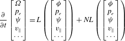 $$\begin{eqnarray}\displaystyle & \displaystyle \frac{\unicode[STIX]{x2202}}{\unicode[STIX]{x2202}t}\left[\begin{array}{@{}c@{}}\unicode[STIX]{x1D6FA}\\ p_{e}\\ \unicode[STIX]{x1D713}\\ v_{\Vert }\\ \cdots \end{array}\right]=L\left(\left[\begin{array}{@{}c@{}}\unicode[STIX]{x1D719}\\ p_{e}\\ \unicode[STIX]{x1D713}\\ v_{\Vert }\\ \cdots \end{array}\right]\right)+NL\left(\left[\begin{array}{@{}c@{}}\unicode[STIX]{x1D719}\\ p_{e}\\ \unicode[STIX]{x1D713}\\ v_{\Vert }\\ \cdots \end{array}\right]\right) & \displaystyle\end{eqnarray}$$
 $$\begin{eqnarray}\displaystyle & \unicode[STIX]{x1D6FA}=\unicode[STIX]{x1D6FB}_{\bot }^{2}\unicode[STIX]{x1D719}, & \displaystyle\end{eqnarray}$$
where fluid moments are used to derive the dynamics in (1.1). The vorticity field
 $\unicode[STIX]{x1D6FA}$
is defined in (1.2). Linear terms are composed of a mix of first and second derivatives and can be seen as a combination of advection and diffusion processes. These processes are associated with resistivity or assumed viscosity of the plasma for the diffusion process. Concerning linear advection, an example is the centrifugal force acting on particles moving around a curved magnetic field. Nonlinear terms correspond typically to a nonlinear advection by a velocity drift (represented by the operator
 $\boldsymbol{u}_{\boldsymbol{D}}\boldsymbol{\cdot }\unicode[STIX]{x1D735}$
) or effects linked to the non-uniformity of the magnetic field which leads to the tearing instabilities (operator
 $\boldsymbol{B}\boldsymbol{\cdot }\unicode[STIX]{x1D735}$
) (see Biskamp Reference Biskamp1993),
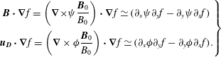 $$\begin{eqnarray}\displaystyle \left.\begin{array}{@{}c@{}}\displaystyle \boldsymbol{B}\boldsymbol{\cdot }\unicode[STIX]{x1D735}f=\left(\unicode[STIX]{x1D735}\times \unicode[STIX]{x1D713}\frac{\boldsymbol{B}_{0}}{B_{0}}\right)\boldsymbol{\cdot }\unicode[STIX]{x1D735}f\simeq (\unicode[STIX]{x2202}_{x}\unicode[STIX]{x1D713}\unicode[STIX]{x2202}_{y}f-\unicode[STIX]{x2202}_{y}\unicode[STIX]{x1D713}\unicode[STIX]{x2202}_{x}f)\\ \displaystyle \boldsymbol{u}_{\boldsymbol{D}}\boldsymbol{\cdot }\unicode[STIX]{x1D735}f=\left(\unicode[STIX]{x1D735}\times \unicode[STIX]{x1D719}\frac{\boldsymbol{B}_{0}}{B_{0}}\right)\boldsymbol{\cdot }\unicode[STIX]{x1D735}f\simeq (\unicode[STIX]{x2202}_{x}\unicode[STIX]{x1D719}\unicode[STIX]{x2202}_{y}f-\unicode[STIX]{x2202}_{y}\unicode[STIX]{x1D719}\unicode[STIX]{x2202}_{x}f).\end{array}\right\} & & \displaystyle\end{eqnarray}$$
The general form of the linear operator is
 $$\begin{eqnarray}\displaystyle L(f)=\frac{\unicode[STIX]{x2202}}{\unicode[STIX]{x2202}x_{i}}[A(\boldsymbol{x})f]+\frac{\unicode[STIX]{x2202}^{2}}{\unicode[STIX]{x2202}x_{i}\unicode[STIX]{x2202}x_{j}}[D(\boldsymbol{x})f], & & \displaystyle\end{eqnarray}$$
where
 $\boldsymbol{x}=\{x_{0},x_{1},\ldots \}$
represents the position vector,
 $A(\boldsymbol{x})$
the advection coefficient and
 $D(\boldsymbol{x})$
the diffusion coefficient. In computational sciences, linear operators are divided into three classes, i.e. hyperbolic, parabolic and elliptic operators. The classification is determined by the nature of the eigenvalues of the associated operator (see Lomax, Pulliam & Zingg Reference Lomax, Pulliam and Zingg2001). The canonical form of an advection process corresponds to a hyperbolic equation, diffusion corresponds to a parabolic equation and elliptic operators correspond to Poisson-type equations. As a consequence, each kind of equation has to be treated with appropriate methods to reproduce accurately the associated mathematical and physical properties. For example, since information propagates with a finite velocity in an advection process but with an infinite velocity in a diffusion process, the methods used in both cases can be different.
The choice of the discretization to advance the evolution of the considered quantities is not unique. Typical possible discretizations are finite difference (FD) approaches, finite elements or spectral methods of Fourier series (see Canuto et al. Reference Canuto, Hussaini, Quarteroni and Zang1988; Ferszinger Reference Ferszinger2002). Only the finite difference approach is discussed here. In general in fusion plasma simulations, a combination of finite differences in the radial direction and Fourier modes in the poloidal and toroidal directions is used (see Jardin Reference Jardin2011). Fourier mode representation gives a higher precision in the numerical schemes, however such a representation can be used only when the geometry is periodic in the considered direction. Another approach concerns the field aligned coordinate systems (see Scott Reference Scott1997), in which case generalized coordinates are used with the property that the grid is aligned to the equilibrium component of the magnetic field.
The methods described in the following for the resolution of partial differential equations (PDE) focus on the FD approach but they can be used also with these other discretizations. The presented properties and limitations remain the same in the framework of these other representations.
An overview of the possible approaches concerning grid decomposition in plasma physics can be found in D’haeseleer (Reference D’haeseleer1991). Many numerical algorithms exist and it may be difficult to decide which one to adopt. The ultimate goal being to obtain the desired accuracy with least effort, or the maximum accuracy with the available resources. In the following sections, typical schemes are detailed, focusing on respective advantages and disadvantages. Section 2 presents the finite difference method, § 3 focuses on the main families of time schemes. These methods are applied to the typical problems of diffusion in § 4 and of advection in § 5. In a last part, the resolution of nonlinear terms is detailed in § 6.
2 Spatial discretization: the finite difference method
Let us consider a general PDE,
 $$\begin{eqnarray}\unicode[STIX]{x2202}_{t}\boldsymbol{u}(\boldsymbol{x},t)=F(\boldsymbol{x},t,\boldsymbol{u},D\boldsymbol{u},D^{2}\boldsymbol{u}),\end{eqnarray}$$
where
 $\boldsymbol{u}(\boldsymbol{x},t)$
is the unknown function,
 $D$
and
 $D^{2}$
are first- and second-order derivatives in space, respectively. The FD approach consists of evaluating the function
 $\boldsymbol{u}(\boldsymbol{x},t)$
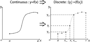
on a discretized domain, as represented in figure 1. The derivatives in the differential equations are replaced by polynomial interpolations. This results in a large algebraic system of equations that has to be solved instead of the differential equation.
Discretization of a function
 $f(x)$
.

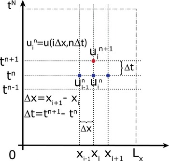
The discretization is made for illustration on a one-dimensional Cartesian grid. Derivation of operators and equations in a generalized system of coordinates appropriate for plasma physics can be found in D’haeseleer (Reference D’haeseleer1991). Equation (2.1) becomes
 $$\begin{eqnarray}\unicode[STIX]{x2202}_{t}u(x,t)=F(x,t,u,\unicode[STIX]{x2202}_{x}u,\unicode[STIX]{x2202}_{x}^{2}u).\end{eqnarray}$$
Unless stated otherwise, the unknown function
 $u(x,t)$
is always assumed to be smooth, meaning that it can be differentiated several times and that each derivative is a well-defined bounded function over an interval containing a particular point of interest
 $x$
.
The cell size or space step is defined by
 $\unicode[STIX]{x0394}x=L_{x}/N=(b-a)/N$
where
 $N$
is the total number of cells in the mesh, with
 $a$
and
 $b$
the left and right border and
 $L_{x}$
the corresponding length. The coordinates of the grid points are then defined by
 $x_{i}=a+\text{i}\unicode[STIX]{x0394}x$
. The solution is computed at each time step
 $\unicode[STIX]{x0394}t$
which corresponds to a series of discrete times
 $t^{n}=n\unicode[STIX]{x0394}t$
,
 $(i,n)\in \mathbb{N}$
.
 $$\begin{eqnarray}u(x,t)\rightarrow u(x_{i},t^{n})\rightarrow u_{i}^{n}.\end{eqnarray}$$
Here,
 $u_{i}^{n}$
corresponds to the value of
 $u(x,t)$
at the position
 $x=a+\text{i}\unicode[STIX]{x0394}x$
and at time
 $t=n\unicode[STIX]{x0394}t$
. To simplify the notation, the superscript
 $n$
is omitted when there is no confusion, e.g.
 $u_{i}$
denotes
 $u_{i}^{n}$
.
Discrete grid used for the function
 $u(x,t)$
.

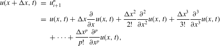
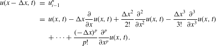
A finite difference scheme is typically obtained by approximating the derivatives in the partial differential equation using a Taylor expansion up to some given order. The minimal order is given by the order of the considered derivative. Generally, the order of a FD scheme, is linked to the rate at which the discretization converges to the exact solution when the step size
 $\unicode[STIX]{x0394}x$
decreases. The error is proportional to
 $(\unicode[STIX]{x0394}x)^{m}$
, where
 $m$
is the exponent of the leading truncation error term. As the values of the unknown function are known only at the grid points, Taylor expansions at different grid points are linearly combined to eliminate all derivatives up to the needed order
 $$\begin{eqnarray}\displaystyle u(x+\unicode[STIX]{x0394}x,t) & = & \displaystyle u_{i+1}^{n}\nonumber\\ \displaystyle & = & \displaystyle u(x,t)+\unicode[STIX]{x0394}x\frac{\unicode[STIX]{x2202}}{\unicode[STIX]{x2202}x}u(x,t)+\frac{\unicode[STIX]{x0394}x^{2}}{2!}\frac{\unicode[STIX]{x2202}^{2}}{\unicode[STIX]{x2202}x^{2}}u(x,t)+\frac{\unicode[STIX]{x0394}x^{3}}{3!}\frac{\unicode[STIX]{x2202}^{3}}{\unicode[STIX]{x2202}x^{3}}u(x,t)\nonumber\\ \displaystyle & & \displaystyle +\cdots +\frac{\unicode[STIX]{x0394}x^{p}}{p!}\frac{\unicode[STIX]{x2202}^{p}}{\unicode[STIX]{x2202}x^{p}}u(x,t),\end{eqnarray}$$
 $$\begin{eqnarray}\displaystyle u(x-\unicode[STIX]{x0394}x,t) & = & \displaystyle u_{i-1}^{n}\nonumber\\ \displaystyle & = & \displaystyle u(x,t)-\unicode[STIX]{x0394}x\frac{\unicode[STIX]{x2202}}{\unicode[STIX]{x2202}x}u(x,t)+\frac{\unicode[STIX]{x0394}x^{2}}{2!}\frac{\unicode[STIX]{x2202}^{2}}{\unicode[STIX]{x2202}x^{2}}u(x,t)-\frac{\unicode[STIX]{x0394}x^{3}}{3!}\frac{\unicode[STIX]{x2202}^{3}}{\unicode[STIX]{x2202}x^{3}}u(x,t)\nonumber\\ \displaystyle & & \displaystyle +\cdots +\frac{(-\unicode[STIX]{x0394}x)^{p}}{p!}\frac{\unicode[STIX]{x2202}^{p}}{\unicode[STIX]{x2202}x^{p}}u(x,t).\end{eqnarray}$$
Using (2.4) and (2.5) the finite difference formulation of the first-order derivative can be expressed as
 $$\begin{eqnarray}\displaystyle & \displaystyle (2.4)\Rightarrow \frac{\unicode[STIX]{x2202}}{\unicode[STIX]{x2202}x}u(x,t)\simeq \frac{u_{i+1}^{n}-u_{i}^{n}}{\unicode[STIX]{x0394}x}+O(\unicode[STIX]{x0394}x), & \displaystyle\end{eqnarray}$$
 $$\begin{eqnarray}\displaystyle & \displaystyle (2.5)\Rightarrow \frac{\unicode[STIX]{x2202}}{\unicode[STIX]{x2202}x}u(x,t)\simeq \frac{u_{i}^{n}-u_{i-1}^{n}}{\unicode[STIX]{x0394}x}+O(\unicode[STIX]{x0394}x). & \displaystyle\end{eqnarray}$$
Equations (2.6) and (2.7) are called forward (FWD), and backward differences (BWD), respectively. These two equations are only first-order approximations (the order of a scheme is linked roughly with the associated error in the numerical representation) which are not sufficient in computational science. Using a combination of (2.4) and (2.5), second-order approximations can be obtained for the first-order derivative, using a central difference (CD) scheme (2.8), and for the second-order derivative, using again a central finite difference scheme (2.9).
 $$\begin{eqnarray}\displaystyle & \displaystyle (2.6)-(2.7)\Rightarrow \frac{\unicode[STIX]{x2202}}{\unicode[STIX]{x2202}x}u(x,t)\simeq \frac{u_{i+1}^{n}-u_{i-1}^{n}}{2\unicode[STIX]{x0394}x}+O(\unicode[STIX]{x0394}x^{2}), & \displaystyle\end{eqnarray}$$
 $$\begin{eqnarray}\displaystyle & \displaystyle (2.6)+(2.7)\Rightarrow \frac{\unicode[STIX]{x2202}^{2}}{\unicode[STIX]{x2202}x^{2}}u(x,t)\simeq \frac{u_{i+1}^{n}+u_{i-1}^{n}-2u_{i}^{n}}{\unicode[STIX]{x0394}x^{2}}+O(\unicode[STIX]{x0394}x^{2}). & \displaystyle\end{eqnarray}$$
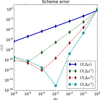
The importance of the scheme order is illustrated in figure 3. FD have been used to compute
 $\text{d}\exp (x)/\text{d}x$
at
 $x=0$
using first-, second-, third- and fourth-order approximations for different step sizes. As the step size decreases, the decrease of the associated error is faster for the higher-order schemes and the numerical solution obtained is more accurate for these schemes. It can be remarked that for very small step size, the error increases, this is not due to the error of the scheme order but due to the finite number of digits used for the representation of decimal numbers.
Relative error in the calculation of
 $\text{d}\exp (x)/\text{d}x$
as a function of the step size using different-order approximations.

This representation is not unique, finite difference approximations can be deduced for any derivatives of
 $u$
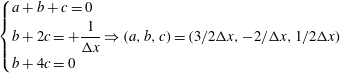
based on a given set of points using the method of undetermined coefficients. As an example, to construct a one-sided FD approximation of
 $\unicode[STIX]{x2202}u/\unicode[STIX]{x2202}x$
based on
 $x_{i},x_{i+1}$
and
 $x_{i+2}$
, let
 $D_{2}u(x)$
be a second-order approximation of
 $\unicode[STIX]{x2202}u/\unicode[STIX]{x2202}x$
,
 $$\begin{eqnarray}D_{2}u(x)=au(x)+bu(x+\unicode[STIX]{x0394}x)+cu(x+2\unicode[STIX]{x0394}x).\end{eqnarray}$$
Using Taylor expansion of
 $u(x+\unicode[STIX]{x0394}x)$
and
 $u(x+2\unicode[STIX]{x0394}x)$
,
 $$\begin{eqnarray}\displaystyle D_{2}u(x) & = & \displaystyle au(x)+bu(x+\unicode[STIX]{x0394}x)+cu(x+2\unicode[STIX]{x0394}x)\end{eqnarray}$$
 $$\begin{eqnarray}\displaystyle & = & \displaystyle (a+b+c)u(x)+(b+2c)\unicode[STIX]{x0394}x\unicode[STIX]{x2202}_{x}u(x)+{\textstyle \frac{1}{2}}(b+4c)\unicode[STIX]{x0394}x^{2}\unicode[STIX]{x2202}_{x}^{2}u(x)\end{eqnarray}$$
 $$\begin{eqnarray}\displaystyle & & \displaystyle +\,{\textstyle \frac{1}{6}}(b+8c)\unicode[STIX]{x0394}x^{3}\unicode[STIX]{x2202}_{x}^{3}u(x)+\cdots\end{eqnarray}$$
This expansion represents
 $\unicode[STIX]{x2202}_{x}u(x)$
if the following relations are satisfied
 $$\begin{eqnarray}\displaystyle & \displaystyle \left\{\begin{array}{@{}l@{}}a+b+c=0\\ b+2c=+\displaystyle \frac{1}{\unicode[STIX]{x0394}x}\Rightarrow (a,b,c)=(3/2\unicode[STIX]{x0394}x,-2/\unicode[STIX]{x0394}x,1/2\unicode[STIX]{x0394}x)\\ b+4c=0\end{array}\right. & \displaystyle\end{eqnarray}$$
 $$\begin{eqnarray}\displaystyle & \displaystyle \unicode[STIX]{x2202}_{x}u_{i}=\frac{-3u_{i}+4u_{i+1}-u_{i+2}}{2\unicode[STIX]{x0394}x}. & \displaystyle\end{eqnarray}$$
3 Schemes for advancing in time
Let us now consider a time-dependent differential equation,
 $$\begin{eqnarray}\unicode[STIX]{x2202}_{t}u(t)=F(t,u(t)).\end{eqnarray}$$
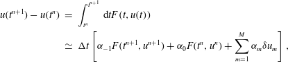
The idea behind any time scheme is based on a numerical quadrature of the associated time integral based on fractional steps (see Rosen Reference Rosen1967) for (3.1):
 $$\begin{eqnarray}\displaystyle u(t^{n+1})-u(t^{n}) & = & \displaystyle \int _{t^{n}}^{t^{n+1}}\,\text{d}tF(t,u(t))\nonumber\\ \displaystyle & \simeq & \displaystyle \unicode[STIX]{x0394}t\left[\unicode[STIX]{x1D6FC}_{-1}F(t^{n+1},u^{n+1})+\unicode[STIX]{x1D6FC}_{0}F(t^{n},u^{n})+\mathop{\sum }_{m=1}^{M}\unicode[STIX]{x1D6FC}_{m}\unicode[STIX]{x1D6FF}u_{m}\right],\end{eqnarray}$$
with
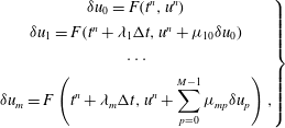 $$\begin{eqnarray}\displaystyle \left.\begin{array}{@{}c@{}}\unicode[STIX]{x1D6FF}u_{0}=F(t^{n},u^{n})\\ \unicode[STIX]{x1D6FF}u_{1}=F(t^{n}+\unicode[STIX]{x1D706}_{1}\unicode[STIX]{x0394}t,u^{n}+\unicode[STIX]{x1D707}_{10}\unicode[STIX]{x1D6FF}u_{0})\\ \cdots \\ \displaystyle \unicode[STIX]{x1D6FF}u_{m}=F\left(t^{n}+\unicode[STIX]{x1D706}_{m}\unicode[STIX]{x0394}t,u^{n}+\mathop{\sum }_{p=0}^{M-1}\unicode[STIX]{x1D707}_{mp}\unicode[STIX]{x1D6FF}u_{p}\right),\end{array}\right\} & & \displaystyle\end{eqnarray}$$
 $\unicode[STIX]{x1D6FC}_{i}$
corresponds to the weight of each expansion coefficient
 $\unicode[STIX]{x1D6FF}u_{i}$
.
Time advance schemes can be classified depending on the value of
 $\unicode[STIX]{x1D6FC}_{-1}$
. If
 $\unicode[STIX]{x1D6FC}_{-1}$
is non-zero, the method is called implicit. At the opposite, if
 $\unicode[STIX]{x1D6FC}_{-1}$
is zero, the method is called explicit. In an explicit method, all terms are evaluated at previous times. As an example, the explicit or forward Euler scheme (EE), which corresponds to
 $\unicode[STIX]{x1D6FC}_{0}=1$
and
 $\unicode[STIX]{x1D6FC}_{i\neq 0}=0$
is expressed by,
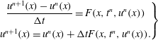 $$\begin{eqnarray}\displaystyle \left.\begin{array}{@{}c@{}}\displaystyle \frac{u^{n+1}(x)-u^{n}(x)}{\unicode[STIX]{x0394}t}=F(x,t^{n},u^{n}(x))\\ u^{n+1}(x)=u^{n}(x)+\unicode[STIX]{x0394}tF(x,t^{n},u^{n}(x)).\end{array}\right\} & & \displaystyle\end{eqnarray}$$
And the implicit version, called implicit or backward Euler (IE), which corresponds to
 $\unicode[STIX]{x1D6FC}_{-1}=1$
and
 $\unicode[STIX]{x1D6FC}_{i\neq -1}=0$
, by
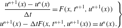 $$\begin{eqnarray}\displaystyle \left.\begin{array}{@{}c@{}}\displaystyle \frac{u^{n+1}(x)-u^{n}(x)}{\unicode[STIX]{x0394}t}=F(x,t^{n+1},u^{n+1}(x))\\ u^{n+1}(x)-\unicode[STIX]{x0394}tF(x,t^{n+1},u^{n+1}(x))=u^{n}(x).\end{array}\right\} & & \displaystyle\end{eqnarray}$$
Moreover, if
 $F$
is linear in
 $u$
, then
 $F(x,t^{n+1},u^{n}(x))=F_{lin}(x,t^{n+1})u^{n}(x)$
and the previous relation can be rewritten as,
 $$\begin{eqnarray}\displaystyle [1-\unicode[STIX]{x0394}tF_{lin}(x,t^{n+1})]u^{n+1}(x)=u^{n}(x). & & \displaystyle\end{eqnarray}$$
Both schemes, implicit and explicit Euler, are only first-order accurate and as a consequence present the same limitations as any first-order scheme. Mainly, the error is proportional to the time step
 $\unicode[STIX]{x0394}t$
and as a consequence, to increase the accuracy by a factor of 10, the time step must be divided by 10 and so the number of iterations is increased by the same amount. Combinations of explicit and implicit schemes can also be used, these schemes are called semi-implicit.
 $$\begin{eqnarray}\displaystyle \left.\begin{array}{@{}c@{}}\displaystyle \frac{u^{n+1}(x)-u^{n}(x)}{\unicode[STIX]{x0394}t}=\unicode[STIX]{x1D703}F(x,t^{n+1},u^{n+1}(x))+(1-\unicode[STIX]{x1D703})F(x,t^{n},u^{n}(x))\\ u^{n+1}(x)-\unicode[STIX]{x1D703}\unicode[STIX]{x0394}tF(x,t^{n+1},u^{n+1}(x))=u^{n}(x)+(1-\unicode[STIX]{x1D703})\unicode[STIX]{x0394}tF(x,t^{n},u^{n}(x))\\ \text{}[1-\unicode[STIX]{x1D703}\unicode[STIX]{x0394}tF_{lin}(x,t^{n+1})]u^{n+1}(x)=[1+(1-\unicode[STIX]{x1D703})\unicode[STIX]{x0394}tF(x,t^{n})]u^{n}(x)\end{array}\right\} & & \displaystyle\end{eqnarray}$$
with
 $0<\unicode[STIX]{x1D703}<1$
. In the case
 $\unicode[STIX]{x1D703}=1/2$
, the method is called Crank–Nicholson (CN) and compared to Euler schemes, this scheme is second-order accurate (the error is reduced quadratically when the step size is decreased).
Each scheme, explicit, implicit and semi-implicit has advantages and disadvantages. In general, implicit schemes are more stable than explicit schemes, where stability can be seen as the property of the solution to remain finite at each time step (this concept is detailed in § 4). However, implicit schemes are more difficult to implement, in particular for nonlinear operators. They also require considerably more calculations than explicit methods and they finally have a poor parallel scalability compared to purely explicit schemes.
The time scheme must be chosen wisely depending on the studied problem as it can affect the physical process described by the equations. To illustrate this, the three schemes presented before (EE, IE and CN) are used to solve the equation describing the one-dimensional (1-D) harmonic oscillator, assuming a unity mass in arbitrary units,
 $$\begin{eqnarray}\unicode[STIX]{x2202}_{t}^{2}x(t)+\unicode[STIX]{x1D714}^{2}x(t)=0.\end{eqnarray}$$
The analytic solution is given by,
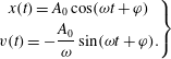 $$\begin{eqnarray}\left.\begin{array}{@{}c@{}}x(t)=A_{0}\cos (\unicode[STIX]{x1D714}t+\unicode[STIX]{x1D711})\\ v(t)=-\displaystyle \frac{A_{0}}{\unicode[STIX]{x1D714}}\sin (\unicode[STIX]{x1D714}t+\unicode[STIX]{x1D711}).\end{array}\right\}\end{eqnarray}$$
Since no damping effects are considered, the total energy of the system, i.e. the sum of kinetic and potential energies, must be conserved during the motion. The total energy is expressed by,
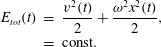 $$\begin{eqnarray}\displaystyle E_{tot}(t) & = & \displaystyle \frac{v^{2}(t)}{2}+\frac{\unicode[STIX]{x1D714}^{2}x^{2}(t)}{2},\nonumber\\ \displaystyle & = & \displaystyle \text{const.}\end{eqnarray}$$
Since the harmonic oscillator is a second-order equation in time, (3.8) should be split into a system of two equations of first order,
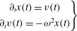 $$\begin{eqnarray}\left.\begin{array}{@{}c@{}}\unicode[STIX]{x2202}_{t}x(t)=v(t)\\ \unicode[STIX]{x2202}_{t}v(t)=-\unicode[STIX]{x1D714}^{2}x(t)\end{array}\right\}\end{eqnarray}$$
and the associated linear systems are,
-
(i) Explicit Euler (EE)
(3.12) $$\begin{eqnarray}\left(\begin{array}{@{}c@{}}x^{n+1}\\ v^{n+1}\end{array}\right)=\left[\begin{array}{@{}cc@{}}1 & \unicode[STIX]{x0394}t\\ -\unicode[STIX]{x1D714}^{2}\unicode[STIX]{x0394}t & 1\end{array}\right]\left(\begin{array}{@{}c@{}}x^{n}\\ v^{n}\end{array}\right).\end{eqnarray}$$
-
(ii) Implicit Euler (IE)
(3.13)
$$\begin{eqnarray}\left[\begin{array}{@{}cc@{}}1 & -\unicode[STIX]{x0394}t\\ \unicode[STIX]{x0394}t\unicode[STIX]{x1D714}^{2} & 1\end{array}\right]\left(\begin{array}{@{}c@{}}x^{n+1}\\ v^{n+1}\end{array}\right)=\left(\begin{array}{@{}c@{}}x^{n}\\ v^{n}\end{array}\right).\end{eqnarray}$$
-
(iii) Crank–Nicholson (CN)
(3.14)
$$\begin{eqnarray}\left[\begin{array}{@{}cc@{}}1 & -\unicode[STIX]{x0394}t/2\\ \unicode[STIX]{x0394}t\unicode[STIX]{x1D714}^{2}/2 & 1\end{array}\right]\left(\begin{array}{@{}c@{}}x^{n+1}\\ v^{n+1}\end{array}\right)=\left[\begin{array}{@{}cc@{}}1 & \unicode[STIX]{x0394}t/2\\ -\unicode[STIX]{x1D714}^{2}\unicode[STIX]{x0394}t/2 & 1\end{array}\right]\left(\begin{array}{@{}c@{}}x^{n}\\ v^{n}\end{array}\right).\end{eqnarray}$$



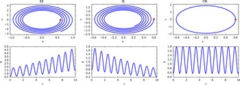
Oscillator motion in
 $x{-}v$
diagram (phase space) and associated time behaviour of the total energy. The red point corresponds to the initial position velocity.

The numerical solutions for the motion of the harmonic oscillator obtained with the three different time schemes are presented in figure 4. The energy conservation property is violated by the explicit and the implicit schemes. Only the CN scheme verifies the energy conservation property of the system. The error in energy conservation of the three schemes can be derived easily starting from (3.10). Posing
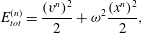 $$\begin{eqnarray}\displaystyle E_{tot}^{(n)}=\frac{(v^{n})^{2}}{2}+\unicode[STIX]{x1D714}^{2}\frac{(x^{n})^{2}}{2}, & & \displaystyle\end{eqnarray}$$
the evolution of
 $E_{tot}^{(t)}$
from
 $t$
to
 $t+1$
should be expressed as a function of
 $E_{tot}^{(t)}$
 $$\begin{eqnarray}\displaystyle E_{tot}^{(n+1)}=\frac{(v^{n+1})^{2}}{2}+\unicode[STIX]{x1D714}^{2}\frac{(x^{n+1})^{2}}{2}. & & \displaystyle\end{eqnarray}$$
Starting from the three linear systems (3.12)–(3.14), and from the calculation of the quantities
 $x$
and
 $v$
at
 $t+\unicode[STIX]{x0394}t$
, the following relations are derived:
-
(i) EE
(3.17)
$$\begin{eqnarray}\displaystyle \left.\begin{array}{@{}c@{}}x^{n+1}=x^{n}+\unicode[STIX]{x0394}tv^{n}\\ v^{n+1}=v^{n}-\unicode[STIX]{x0394}t\unicode[STIX]{x1D714}^{2}x^{n}\\ \Rightarrow E_{tot}^{(n+1)}=\left(1+\unicode[STIX]{x0394}t^{2}\unicode[STIX]{x1D714}^{2}\right)E_{tot}^{(n)}>E_{tot}^{(n)}.\end{array}\right\} & & \displaystyle\end{eqnarray}$$
-
(ii) IE
(3.18)
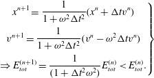
$$\begin{eqnarray}\displaystyle \left.\begin{array}{@{}c@{}}\displaystyle x^{n+1}=\frac{1}{1+\unicode[STIX]{x1D714}^{2}\unicode[STIX]{x0394}t^{2}}(x^{n}+\unicode[STIX]{x0394}tv^{n})\\ \displaystyle v^{n+1}=\frac{1}{1+\unicode[STIX]{x1D714}^{2}\unicode[STIX]{x0394}t^{2}}(v^{n}-\unicode[STIX]{x1D714}^{2}\unicode[STIX]{x0394}tv^{n})\\ \displaystyle \Rightarrow E_{tot}^{(n+1)}=\frac{1}{(1+\unicode[STIX]{x0394}t^{2}\unicode[STIX]{x1D714}^{2})}E_{tot}^{(n)}<E_{tot}^{(n)}.\end{array}\right\} & & \displaystyle\end{eqnarray}$$
-
(iii) CN
(3.19)
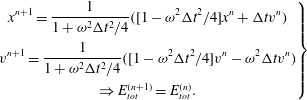
$$\begin{eqnarray}\displaystyle \left.\begin{array}{@{}c@{}}\displaystyle x^{n+1}=\frac{1}{1+\unicode[STIX]{x1D714}^{2}\unicode[STIX]{x0394}t^{2}/4}([1-\unicode[STIX]{x1D714}^{2}\unicode[STIX]{x0394}t^{2}/4]x^{n}+\unicode[STIX]{x0394}tv^{n})\\ \displaystyle v^{n+1}=\frac{1}{1+\unicode[STIX]{x1D714}^{2}\unicode[STIX]{x0394}t^{2}/4}([1-\unicode[STIX]{x1D714}^{2}\unicode[STIX]{x0394}t^{2}/4]v^{n}-\unicode[STIX]{x1D714}^{2}\unicode[STIX]{x0394}tv^{n})\\ \Rightarrow E_{tot}^{(n+1)}=E_{tot}^{(n)}.\end{array}\right\} & & \displaystyle\end{eqnarray}$$
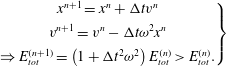
The violation of the energy conservation for IE and EE schemes appears via a second-order term in
 $\unicode[STIX]{x0394}t$
. Analytical calculation shows that the observed energy growth is not linked to an inappropriate value of the time step but directly to the numerical properties of the scheme. The implicit scheme however introduces artificial damping from the truncations which leads to a decrease of the energy of the system. Advantages of this numerical dissipation is an increased stability compared to explicit schemes. The associated consequences are described in § 4. The properties of the described system allows to express it as an Hamiltonian operator:
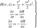 $$\begin{eqnarray}\displaystyle \left.\begin{array}{@{}c@{}}\displaystyle H(v,x)=\frac{v^{2}}{2}+\frac{\unicode[STIX]{x1D714}^{2}}{2}x^{2},\\ {\displaystyle \frac{\unicode[STIX]{x2202}v}{\unicode[STIX]{x2202}t}}={\displaystyle \frac{\unicode[STIX]{x2202}H}{\unicode[STIX]{x2202}x}}\\ {\displaystyle \frac{\unicode[STIX]{x2202}x}{\unicode[STIX]{x2202}t}}=-{\displaystyle \frac{\unicode[STIX]{x2202}H}{\unicode[STIX]{x2202}v}}.\end{array}\right\} & & \displaystyle\end{eqnarray}$$
The energy conservation observed with the CN scheme is related to a property of this integrator which is that to be a symplectic integrator, this class of integrators preserves the properties of the associated Hamiltonian (e.g. energy conservation or geometrical properties). In Hairer (Reference Hairer2006), more details and possible schemes for such systems are presented.
3.1 Typical time advance schemes used
Euler schemes are generally not satisfying for the numerical resolution of PDEs. Even if their implementation is simple and fast, these schemes are only of first-order accuracy. Higher-order schemes have been developed (see Durran Reference Durran2010) and can be divided in two families:
(i) schemes which use information at steps
 $t,t-\unicode[STIX]{x0394}t,\ldots$
to calculate the solution at time
 $t+\unicode[STIX]{x0394}t$
. The main schemes used are Adams–Moulton (AM) and Adams–Bashforth (AB) schemes. AM are implicit linear multistep methods and AB is explicit. A variant of AB used in plasma physic is the time scheme developed by Karniadakis, Israeli & Orszag (Reference Karniadakis, Israeli and Orszag1991). Compared to the original AB schemes, this one has a better accuracy and an increased stability region. The third-order explicit version of the scheme is given here
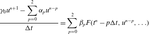 $$\begin{eqnarray}\displaystyle & \displaystyle \frac{\displaystyle \unicode[STIX]{x1D6FE}_{0}u^{n+1}-\mathop{\sum }_{p=0}^{2}\unicode[STIX]{x1D6FC}_{p}u^{n-p}}{\unicode[STIX]{x0394}t}=\mathop{\sum }_{p=0}^{2}\unicode[STIX]{x1D6FD}_{p}F(t^{n}-p\unicode[STIX]{x0394}t,u^{n-p},\ldots ) & \displaystyle\end{eqnarray}$$
 $$\begin{eqnarray}\displaystyle & \unicode[STIX]{x1D6FC}_{p}=3,-3/2,1/3 & \displaystyle\end{eqnarray}$$
 $$\begin{eqnarray}\unicode[STIX]{x1D6FD}_{p}=3,-3,1,\quad \unicode[STIX]{x1D6FE}_{0}=11/6.\end{eqnarray}$$
In the case where one of the operators present in
 $F$
corresponds to a diffusion operator with a coefficient
 $\unicode[STIX]{x1D708}$
(
 $\unicode[STIX]{x1D708}\unicode[STIX]{x1D6FB}^{2}$
), an implicit version exists. The implicit version consist mainly in an implicit treatment of the diffusion operator, the advantage of the implicit diffusion is an increased stability region for the scheme due to damping of associated high wavenumbers:
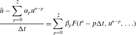 $$\begin{eqnarray}\displaystyle & \displaystyle \frac{\displaystyle \hat{u} -\mathop{\sum }_{p=0}^{2}\unicode[STIX]{x1D6FC}_{p}u^{n-p}}{\unicode[STIX]{x0394}t}=\mathop{\sum }_{p=0}^{2}\unicode[STIX]{x1D6FD}_{p}F(t^{n}-p\unicode[STIX]{x0394}t,u^{n-p},\ldots ) & \displaystyle\end{eqnarray}$$
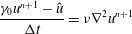 $$\begin{eqnarray}\displaystyle & \displaystyle \frac{\unicode[STIX]{x1D6FE}_{0}u^{n+1}-\hat{u} }{\unicode[STIX]{x0394}t}=\unicode[STIX]{x1D708}\unicode[STIX]{x1D6FB}^{2}u^{n+1} & \displaystyle\end{eqnarray}$$
 $$\begin{eqnarray}\displaystyle & \unicode[STIX]{x1D6FC}_{p}=3,-3/2,1/3 & \displaystyle\end{eqnarray}$$
 $$\begin{eqnarray}\unicode[STIX]{x1D6FD}_{p}=3,-3,1,\quad \unicode[STIX]{x1D6FE}_{0}=11/6.\end{eqnarray}$$
(ii) schemes where the right-hand side term is approximated at intermediate times between
 $t$
and
 $t+\unicode[STIX]{x0394}t$
. This principle is used in the elaboration of the Runge–Kutta (RK) schemes. RK schemes are not unique at each order, the choice depends on the desired properties for the system (see Shu & Osher Reference Shu and Osher1988; Butcher Reference Butcher2008). As computer performances have increased during the last years, fourth-order RK schemes are actually used widely,
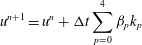 $$\begin{eqnarray}\displaystyle & \displaystyle u^{n+1}=u^{n}+\unicode[STIX]{x0394}t\mathop{\sum }_{p=0}^{4}\unicode[STIX]{x1D6FD}_{p}k_{p} & \displaystyle\end{eqnarray}$$
 $$\begin{eqnarray}\displaystyle & \displaystyle k_{p}=F\left(t^{n}+c_{p}\unicode[STIX]{x0394}t,u^{n}+\unicode[STIX]{x0394}t\mathop{\sum }_{q=0}^{4}\unicode[STIX]{x1D6FC}_{nq}k_{q}\right). & \displaystyle\end{eqnarray}$$
4 Numerical modelling of diffusion
The diffusion equation with a constant diffusion coefficient
 $D$
(also called the heat equation) is the simplest parabolic PDE. The time evolution of the positive definite field
 $u(x,t)$
is given by,
 $$\begin{eqnarray}\unicode[STIX]{x2202}_{t}u(x,t)=D\unicode[STIX]{x2202}_{x}^{2}u(x,t).\end{eqnarray}$$
Using a second-order scheme in space, the right-hand side of (4.1) is discretized using a central expression,
 $$\begin{eqnarray}D\unicode[STIX]{x2202}_{x}^{2}u(x,t)\simeq D\frac{u_{i+1}+u_{i-1}-2u_{i}}{\unicode[STIX]{x0394}x^{2}}.\end{eqnarray}$$
4.1 Stability analysis and Courant–Friedrichs–Lewy (CFL) condition
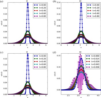
Numerical simulations have been realized with IE and EE schemes and spatial CD, respectively. The obtained profiles for
 $u(x,t)$
at different times are plotted in figure 5. Two runs with two different time steps are performed in both cases. Obviously, the implicit Euler scheme produces nearly identical results with both time steps whereas the results obtained with the explicit Euler scheme are strongly affected by the choice of the time step. Here, for the larger time step, the solution
 $u(x,t)$
shows an oscillating behaviour with an exponential growth. This behaviour can be explained through the corresponding stability analysis.
Solution obtained for the diffusion equation with
 $N_{x}=256,L_{x}=2\unicode[STIX]{x03C0}$
.
 $\unicode[STIX]{x0394}t=5e{-}4$
for cases (a) and (b) and
 $\unicode[STIX]{x0394}t=8e{-}4$
for cases (c) and (d).

The stability property of a time advancing scheme can be studied through the Von Neumann stability analysis technique (see Durran Reference Durran2010). Note that it is very important to realize that the stability of a scheme is different from its accuracy. To be useful, a numerical scheme must be both consistent and stable.
Consistency means that, the (continuous) solution of the PDE must satisfy the discretized version of the equation – using the respective time scheme – with approximation errors that vanish when
 $\unicode[STIX]{x0394}x$
and
 $\unicode[STIX]{x0394}t$
approach zero. Consistency guarantees that the scheme truly approximates the equation intended to be solved (and not something else).
Stability means that the scheme does not amplify errors. Obviously, this is very important, since truncation errors are impossible to avoid in any numerical calculation. In fact, even in the ideal case of infinite precision, some errors (e.g. discretization errors) remain. Clearly, if errors are amplified, they will rapidly dominate any computation (making it useless). In the simplest case of linear constant coefficient schemes, a complete stability analysis is possible as the numerical algorithm equations can be solved exactly by separation of variables. It follows that any solution of these equations can be written as a superposition of Fourier modes. Since these Fourier modes are uncoupled, the evolution of each mode can be considered individually. As an example, considering (4.1), the field
 $u(x,t)$
can be expressed as a sum of complex wave functions. For an infinite space, the initial condition can be written as,
 $$\begin{eqnarray}u(x,t=0)=u_{0}(x)=\frac{1}{\sqrt{2\unicode[STIX]{x03C0}}}\int _{-\infty }^{\infty }\tilde{u} (k)\text{e}^{\text{i}kx}\,\text{d}k.\end{eqnarray}$$
Let us assume moreover, that the initial condition, for simplicity, can be expressed using only one Fourier mode,
 $$\begin{eqnarray}u(x,t=0)\rightarrow u_{j}^{0}=U_{0}\text{e}^{\text{i}kj\unicode[STIX]{x0394}x}.\end{eqnarray}$$
After a single application of the differencing scheme, the mode’s amplitude and phase are modified by a factor
 $G(k)$
,
 $$\begin{eqnarray}\text{e}^{\text{i}kj\unicode[STIX]{x0394}x}\rightarrow G(k)\text{e}^{\text{i}kj\unicode[STIX]{x0394}x},\end{eqnarray}$$
and after
 $n$
iterations, the field at time
 $(t_{n}=n\unicode[STIX]{x0394}t)$
has the form
 $$\begin{eqnarray}u_{j}^{n}=G^{n}(k)u_{j}^{0},\end{eqnarray}$$
where
 $G(k)$
corresponds to the complex amplification factor of the scheme. A scheme is stable only if an initial error is not amplified, which corresponds to
 $|G(k)|\leqslant 1$
. More precisely, if
 $|G(k)|=1$
, the scheme is classified as neutral and if
 $|G(k)|<1$
, the scheme is damping. From this analysis, it is found that the EE scheme has an amplification factor expressed by,
 $$\begin{eqnarray}G(k)=1-4\frac{D\unicode[STIX]{x0394}t}{\unicode[STIX]{x0394}x^{2}}\sin ^{2}\left(\frac{k\unicode[STIX]{x0394}x}{2}\right).\end{eqnarray}$$
From the above condition, the scheme is stable only if
 $$\begin{eqnarray}\frac{D\unicode[STIX]{x0394}t}{\unicode[STIX]{x0394}x^{2}}\leqslant \frac{1}{2}.\end{eqnarray}$$
In contrast, for the IE scheme, the amplification factor is
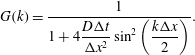 $$\begin{eqnarray}G(k)=\frac{1}{1+4\displaystyle \frac{D\unicode[STIX]{x0394}t}{\unicode[STIX]{x0394}x^{2}}\sin ^{2}\left(\displaystyle \frac{k\unicode[STIX]{x0394}x}{2}\right)}.\end{eqnarray}$$
Since,
 $|G(k)|\leqslant 1\,\forall \unicode[STIX]{x0394}t,\unicode[STIX]{x0394}x>0$
, this scheme is unconditionally stable.
The value of
 $|G(k)|$
for the explicit Euler is mainly governed by the number
 $n_{c}=D\unicode[STIX]{x0394}t/\unicode[STIX]{x0394}x^{2}$
. For the results presented above, the first value of the time step corresponds to
 $n_{c}=0.42$
and the second value to
 $n_{c}=0.68$
. As expected, the second case is unstable,
 $n_{c}=0.68>1/2$
. The number
 $n_{c}$
is called in the literature the Courant number. The stability condition is associated with the so called Courant–Friedrichs–Lewy condition (see Courant, Friedrichs & Lewy Reference Courant, Friedrichs and Lewy1928). However this is true mainly only for the single stage linear methods such as the Euler scheme. In general, the CFL condition is necessary but not sufficient to ensure stability (see Schneider, Kolomenskiy & Deriaz Reference Schneider, Kolomenskiy and Deriaz2013).
A physical interpretation of the unconditional stability of the implicit Euler scheme is linked to the fact that this method avoids growth of small scales through an artificial damping of these scales.
The treatment of diffusion is a challenge in plasma physics computations. The first issue with respect to the diffusion process, which is not detailed here, is the strong anisotropy of diffusion between the directions parallel and perpendicular to the magnetic field. Here, splitting between explicit and implicit operators should be implemented to treat correctly both directions with an acceptable time step (see Crouseilles, Kuhn & Latu Reference Crouseilles, Kuhn and Latu2015).
The constraint is not on the diffusion coefficient (which is typically quite small (see Freidberg Reference Freidberg2007)) but the correct treatment of small scales. The presence of small scales requires a fine grid with small
 $\unicode[STIX]{x0394}x$
. In a 1-D simulation, decreasing
 $\unicode[STIX]{x0394}x$
e.g. by a factor of
 $4$
for example, implies that
 $\unicode[STIX]{x0394}t$
needs to be divided by
 $16$
. As a consequence, for the same simulation, the simulation time will be
 $16\times 4=64$
times longer. Increasing grid resolution has an important impact on the simulation time, which is even worst in 3-D; an increased resolution by a factor 4 in each direction leads to a computational time
 $16\times 4^{3}=1024$
times higher. A consequence of this is that simulations cannot be done anymore on simple workstations but must use parallel computers.
The simple diffusion equation is used as a starting point for an illustration of parallel implementations based on a purely serial code. Possible parallel implementations can be divided into two families depending on the hardware used for the simulations. Both implementation and how to develop them from a serial code are presented in the following sections.
4.2 Numerical implementation
4.2.1 Performance measurement
Before presentation of possible numerical implementations applied to the resolution of parabolic equations, it is important to define a way to characterize benefits associated with parallel implementations with respect to the serial one. Performance gain can be both modelled and measured. In this section we will take a another look at parallel computations by giving a simple analytical model that illustrates some of the factors that influence the performance of a parallel program. Consider a program consisting of three parts: an initialization section (time
 $T_{i}$
), a computation section (time
 $T_{c}$
) and a finalization section (time
 $T_{f}$
). The total running time of this program on one processor (called the serial version) is then given as the sum of the times for the three parts:
 $$\begin{eqnarray}T_{s}=T_{i}+T_{c}+T_{f}.\end{eqnarray}$$
Now, how will this running time evolve when the program is run in parallel? Assuming that the program is run on
 $P$
processors and that
 $T_{i}$
and
 $T_{f}$
are almost independent of the number of processors, the parallel time
 $T_{p}$
ideally becomes, in particular if the influence of the communication cost between processors is neglected:
 $$\begin{eqnarray}T_{p}(P)=T_{i}+T_{c}/P+T_{f}.\end{eqnarray}$$
The performance gain is measured by the speed-up
 $S(P)$
which describes how much faster a problem runs. The actual running time does not appear and the speed-up
 $S(P)$
is normalized such that
 $$\begin{eqnarray}S(P)=T_{s}/T_{p}(P).\end{eqnarray}$$
Defining
 $\unicode[STIX]{x1D6FE}$
as,
 $$\begin{eqnarray}\displaystyle \unicode[STIX]{x1D6FE}=\frac{T_{i}+T_{f}}{T_{s}}, & & \displaystyle\end{eqnarray}$$
 $S(P)$
is simplified as,
 $$\begin{eqnarray}S(P)=1/(\unicode[STIX]{x1D6FE}+(1-\unicode[STIX]{x1D6FE})/P).\end{eqnarray}$$
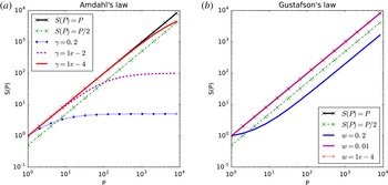
Equation (4.14) is well known as Amdahl’s law (see Amdahl Reference Amdahl1967) and says that, in absence of unparallelized parts (
 $\unicode[STIX]{x1D6FE}=0$
), speed-up scales as the number of processors used for the simulation. This case is defined as an ideal speed-up. However, as can be seen in figure 6, the serial part is a highly limiting factor in the scalability of a code. For example, with
 $\unicode[STIX]{x1D6FE}=0.5$
(which means that 50 % of the code cannot be run in parallel), using 4 processors gives a speed-up of 1.6, far away from the
 $S=4$
desired. This constraint leads to a strong limitation on the parallel scalability of a code. As observed in figure 6, with
 $\unicode[STIX]{x1D6FE}=1\,\%$
, passing from 100 to 1000 processors gives only a negligible gain in running time. And as consequence, Amdahl’s law appears as a strong limitation on performance increases of codes with an increasing number of processors used. This conclusion has been softened by Gustafson (see Gustafson Reference Gustafson1988) who stated that if the serial part cannot be reduced, it is possible to solve a larger problem efficiently in the same amount of time. As the problem size grows, the work required for the parallel part of the problem frequently grows much faster compared to that required for the serial part, then as the problem size grows, the serial fraction decreases and the speed-up improves. In Gustafson’s law, the speed-up follows the rule:
 $$\begin{eqnarray}S(P)=w+(1-w)\ast P,\end{eqnarray}$$
with
 $w$
being the part which benefits from resources improvement (as illustrated in figure 6
b). These performance measurements and associated conclusions will be used in the following section, illustrating 2 different parallel implementations to solve a 1-D diffusion equation.
Speed-up as function of number of processors, using Amdahl’s (a) and Gustafson’s (b) laws.

4.2.2 Serial implementation
Starting point is the resolution of the diffusion equation with a constant source term. For this purpose, a second-order central derivative for the Laplacian operator is used,
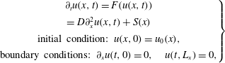 $$\begin{eqnarray}\left.\begin{array}{@{}c@{}}\unicode[STIX]{x2202}_{t}u(x,t)=F(u(x,t))\\ =D\unicode[STIX]{x2202}_{x}^{2}u(x,t)+S(x)\\ \text{initial condition: }u(x,0)=u_{0}(x),\\ \text{boundary conditions: }\unicode[STIX]{x2202}_{x}u(t,0)=0,\quad u(t,L_{x})=0,\end{array}\right\}\end{eqnarray}$$
where
 $D\unicode[STIX]{x2202}_{x}^{2}u(x,t)$
is discretized by
 $$\begin{eqnarray}D\unicode[STIX]{x2202}_{x}^{2}u(x,t)\Rightarrow D\frac{u_{i+1}+u_{i-1}-2u_{i}}{\unicode[STIX]{x0394}x^{2}}.\end{eqnarray}$$
The time evolution is resolved by a fourth-order Runge–Kutta scheme (RK-4),
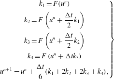 $$\begin{eqnarray}\left.\begin{array}{@{}c@{}}k_{1}=F(u^{n})\\ \displaystyle k_{2}=F\left(u^{n}+\frac{\unicode[STIX]{x0394}t}{2}k_{1}\right)\\ \displaystyle k_{3}=F\left(u^{n}+\frac{\unicode[STIX]{x0394}t}{2}k_{2}\right)\\ \displaystyle k_{4}=F\left(u^{n}+\unicode[STIX]{x0394}tk_{3}\right)\\ \displaystyle u^{n+1}=u^{n}+\frac{\unicode[STIX]{x0394}t}{6}(k_{1}+2k_{2}+2k_{3}+k_{4}),\end{array}\right\}\end{eqnarray}$$
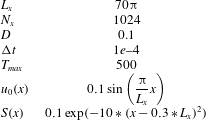
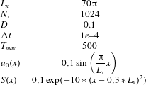
to yield the discrete equation. For the simulations, the reference numerical set-up used in § 4.2 is indicated in table 1.
Reference numerical set-up for the resolution of (4.16).
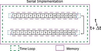
A serial implementation of a such model (serial implementation means a version of the numerical code which can be executed only on
 $1$
core) is illustrated in figure 7. The field
 $u(x,t)$
is modelled through an array in which each cell contains the value of
 $u$
at a given time
 $t$
for all spatial grid points. In the case sketched in figure 7, the spatial grid contains 16 cells numbered from 0 to 15. The right-hand side of (4.16) is represented by a function
 $F$
which is applied to every element of the array
 $u$
using a RK-4 algorithm (4.18). RK-4 needs 4 intermediate arrays which are not represented on figure 7 for simplicity.
The corresponding implementation of the time loop is presented in listing 1.

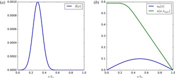
Figure 8 shows on the left the included source and on the right the initial and final profiles obtained at
 $t=T_{max}$
.
Data storage in memory in a serial implementation, the arrow represent the computation of
 $u$
at
 $t+\unicode[STIX]{x0394}t$
in function of
 $u$
at
 $t$
.

Source profile (a) and initial/final field for numerical simulation (b) of (4.16).

4.2.3 Message passing interface (MPI) implementation
The previous code can be greatly accelerated not through low-level optimizations but by taking advantage of modern computers architecture. For that purpose, the development of a parallel version using an MPI library (see Message Passing Interface Forum 2015) is explained. MPI can be seen as a way to execute a software as a set of processes that have only local memory but are able to communicate with other processes by sending and receiving messages. MPI has been designed mainly to be used with a distributed collection of machines. An MPI program can be divided into 3 parts
-
(i) initialization through the MPI_Init function;
-
(ii) program core;
-
(iii) termination of parallel part with the MPI_Finalize command.
Since the evaluation of
 $u$
at time
 $t^{n+1}=t^{n}+\unicode[STIX]{x0394}t$
depends on its value at time
 $t^{n}$
, the time loop cannot be parallelized. The only part which can be parallelized is the calculation of the Laplacian of
 $u$
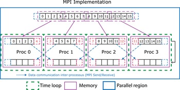
. For the following description of the method, the simulation is considered to be run on 4 processes. In the serial algorithm, all the data are stored in the memory of the execution process. This concept cannot be used in an MPI version: if only 1 process can access the data, the other processes are useless. At the opposite, sending all the information to all processes generates an unnecessary memory allocation when the number of CPU (central processing unit) increases. As consequence, for the MPI version, the spatial domain is divided between available processes. Each process can access only its associated memory and has access only to a part of the full domain as presented in figure 9. Since each process knows only a part of the grid, it is necessary to communicate values of ‘local’ boundaries between processes. These local boundaries, often called ghost points in the literature, correspond to artificial points added during the grid decomposition step. These points are used as buffer for received values from other process. Communications (dashed arrows) are made through calls to MPI functions MPI_Send and MPI_IRecv (see Message Passing Interface Forum 2015).
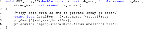
With MPI, communications between processes must be made explicitly in the code, indicating which process sends the data and which one should receive them. As a first part, and before the time loop, a ‘map’ of the processes is generated and each process can know which processes are his left and right neighbours. Generally, this part concerning the creation of the topology for the communications is made with the MPI_Cart_Create function but for the purpose of this paper, a simple implementation is made. A structure containing the necessary information is initialized, as presented in listing 2. Using the concept of ghost points previously described, this explains why, on line 34 of listing 2, 2 cells are added to the local size of the corresponding domain.

Once the topology is initialized, the next step is to scatter the data between all processes. This is made with the MPI_Scatter function called inside the function MPI_global2local (see § C.2 for the implementation). Compared to the serial version, each process needs updated values for the local boundaries coming from neighbours. As a consequence, the serial function Generate_BC is replaced by a function MPI_Copy_BC which manages the communications for each intermediate step of the RK-4 implementation. For process
 $m$
, the goal is to send and receive at the same time values from processes
 $m-1$
and
 $m+1$
. To avoid the problem of a deadlock in this function, (a deadlock is a situation in which two or more competing actions are each waiting for the other to finish, and thus neither ever does), non-blocking functions represented by the ‘_I’ in function names are used. This allows each process to wait for data reception from a process and at the same time, send data to another process.

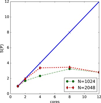
With this implementation, the speed-up
 $S(P)$
is represented in figure 10. All simulations have been performed on a cluster node with 2 processors of 10 cores. On this cluster, speed-up tends to a limit value around 2.5–3 for both resolutions. The measured speed-up tends to reach the ideal one when the resolution increases. Higher resolution generates more operations at each time step, and, since in the presented algorithm the communication cost is independent of the resolution, the obtained speed-up is higher: as expected in Gustafson’s law, the ratio communication/computation decreases leading to better performances. In the simulation made to study physical models, the number of operators and considered resolutions are higher than the ones presented here, this leads to a better scaling with a simple domain decomposition method.
MPI implementation sketching computation from time
 $t^{n}$
to time
 $t^{n+1}$
.

Speed-up
 $S(P)$
obtained using MPI implementation. The solid line corresponds to the ideal case (
 $S(P)=P$
) and dashes lines to the measured values for resolutions of 1024 and 2048 points.

MPI was first defined for distributed memory architectures. However, modern clusters are a combination of distributed memory between nodes but each node can be assimilated as a shared memory system. Even if MPI can take advantage of a shared memory environment, another library, OpenMP, is used to present another possible implementation. The choice of OpenMP library is that this library is dedicated to the development of parallel programs on shared memory architectures.
4.2.4 OpenMP implementation
OpenMP (see Chapman, Jost & Van der Pas Reference Chapman, Jost and Van der Pas2007) standard was formulated in 1997 as a set of library routines and tools for writing portable multiprocessing computer programs. Any computer program can be considered as a set of processes (or threads) and OpenMP permits for example to balance the total calculation between the different processes.
OpenMP provides a platform-independent set of compiler pragmas (a pragma is a language construct that specifies how a compiler should process the input source code), directives, function calls and environment variables that explicitly instruct the compiler how and where to use parallelism in the application. The method is well suited for domain (and/or loop) decomposition. The possible OpenMP implementations differ depending on the level of granularity considered in the algorithm. Granularity can be defined as the ratio between the amount of computations executed by a thread and the amount of communications between threads. Fine-grained parallelism means that individual tasks are relatively small in terms of code size and execution time. The data are frequently transferred between processors in amounts of one or a few memory words. The coarse-grained approach is the opposite: data are communicated infrequently, after larger amounts of computation. The finer the granularity, the larger is the potential for parallelism and hence speed-up, but the larger are also the overheads of synchronization and communication. As for MPI implementation, this last point is the critical issue for obtaining an effective speed-up.
The fine-graining technique uses OpenMP directives directly in loops to produce a parallel version of the code at compilation time. The following example shows the corresponding implementation for computation of the Laplacian operator.
Let
 $u(x,t)$
be discretized on
 $N$
points in space, the extrema points with index
 $i=0$
and respectively
 $i=N-1$
, are used as ‘ghost’ points implied by the boundary conditions. The numerical implementation is as follows,
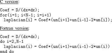
To obtain a parallel version of the loop, using OpenMP, only one directive has to be added in front of the loop.
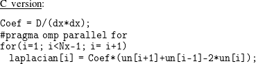
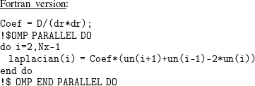
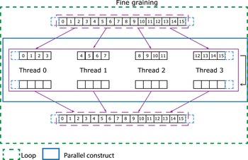
Fine-graining decomposition is illustrated in figure 11 assuming 4 available threads for the simulation. Compared to the MPI implementation, this time the field is not distributed between processes, each core has access to the full field but loop iterations are divided between cores.
Fine-graining method. Arrows indicates scattering and gathering of data between cores through OpenMP directives (4 cores and 16 points are considered here).

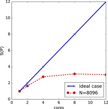
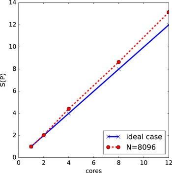
The dashed rectangle represents the do/for loop and the blue rectangle the parallel region. Since each threads runs in parallel, the calculation time is expected to be divided by 4 compared to the serial case. In figure 12, the speed-up
 $S(P)$
is plotted for an input array of
 $N=8096$
elements. The speed-up is close to the theoretical one from 1 and 2 threads, but for more threads, there is a saturation close to a speed-up of 3. Our test case is rather simple and with increasing number of threads, the computational costs linked to the generation and destruction of threads, to the sharing of variables between them and to the associated communications are not negligible anymore. Therefore, this simple example shows that an efficient implementation of an OpenMP structure in a given code cannot be sketched to a simple addition of directives before loops. To be efficient, the directives should be made in the loops which have a large number of calculations per iteration.
Measured speed-up for a fine-graining implementation of OpenMP directives.

OpenMP can also be implemented in a coarse-graining approach. This approach can be seen as a way to simulate an MPI implementation with OpenMP directives. Generally, for parallel numerical tools, domain decomposition is made using MPI techniques, and OpenMP fine-graining techniques are used as a refinement. However, as it has been shown in the previous section, the performances of the fine-graining approach are strongly linked to the number of operations in each loop. Typically, for complicated models, the corresponding code will have many loops with few operations for each. This is due to the choices of the decomposition for each direction for example or the resolutions used in 3-D and the associated simulation time. For this kind of simulation, pure MPI implementation has generally better performance and scaling than an equivalent code mixing MPI domain decomposition and OpenMP fine graining. However, this kind of OpenMP implementation becomes more and more interesting since the generations of cluster nodes or even workstations have between 4 to 16 or even more cores per nodes. Compared to the fine graining where the parallelism is operated at a loop level, coarse graining is more intrusive.
In a coarse-graining (CG) approach, the domain decomposition is operated from the beginning and communications between processes are made explicitly. Understanding CG implementation with OpenMP directives requires a more precise description of the memory environment in an OpenMP process (see Chapman et al. Reference Chapman, Jost and Van der Pas2007).
A program can be divided into smaller sequences of codes which can be managed independently, each one of this sequence is called a thread. OpenMP assumes that in a shared memory environment, all threads can access the same memory for storing and retrieving data. Each thread may have a private, temporary view of the memory (called a thread’s view) at the beginning of an OpenMP construct (a parallel region) that it can use instead of the memory to store data during its execution when these data do not need to be seen by other threads.
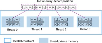
Data can be ‘transferred’ between the memory and a thread’s view, but can never move between temporary views directly, without going through the memory. Each variable used within a parallel region is either shared or private. Each shared variable reference inside a parallel region refers to the original variable of the same name. For each private variable, a reference to the variable name refers to a variable of the same type and size as the original variable, but private to the thread. It is therefore not accessible by other threads. The elaboration of a communication-like system in such a case is described in the following using again the example of the diffusion equation. As in previous sections, a decomposition on 4 threads with spatial discretization on 16 points is used. As in the MPI version, the parallelization starts in that case from the initialization: values for
 $u_{0},u_{1},u_{2},u_{3}$
are stored on thread 0, values for
 $u_{4},u_{5},u_{6},u_{7}$
are stored on thread
 $1,\ldots$
and values for
 $u_{12},u_{13},u_{14},u_{15}$
are stored on thread 3. Since each thread contains its own version of the variable with the same name, we distinguish them using the thread number as a superscript.
 $A_{0}^{[0]}$
corresponds to the value of
 $A_{0}$
for the thread 0,
 $A_{0}^{[1]}$
corresponds to the value of
 $A_{0}$
for the thread
 $1\ldots$
. This concept is illustrated on figure 13.
The starting point is the creation of an equivalent to a 1-D topology. A similar structure as the one used in § 4.2.3 is declared and initialized. Each thread is identified with a unique number starting from 0 and increased by 1 for each thread. The structure itself is similar to the one used for MPI, the difference is the calling function giving unique identity of the thread. This identity is used to create the notion of neighbours for each thread, as in the MPI case.

Once the initialization is completed, data have to be scattered between threads. This part is illustrated in listing 4, only the case of the array corresponding to the source term is represented. For clarity, variable names starting with g_ correspond to the original variables and names starting with pr_ are associated with the thread private view.
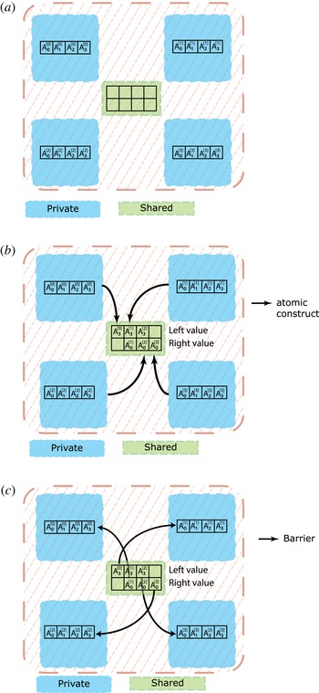
Schematic representation of the coarse-graining communication process.


The most complex part is the simulation of a communication mechanism like send/receive using OpenMP directives. The previous mechanism based on the functions OMP_global2local and OMP_local2global (function defined in § C.3) cannot be used in the time loop. The associated communication cost is too important and as a consequence the scalability is poor and not efficient at all.
The developed technique is based on two other pragma directives defined in OpenMP (see OpenMP 2015):
-
(i) atomic: ensure that only one thread at a time accesses a shared variable, and subsequently synchronize updated contents with all other threads view,
-
(ii) barrier: synchronizes all threads, acts like a breakpoint that all threads must reach before execution of other instructions.
Since each thread knowns only a part of the grid, the values of the local boundaries have to be updated at each iteration due to the stencil used for spatial derivatives. For example, the Laplacian at grid node
 $i=4$
is based on values of
 $u$
at position
 $i=3,4,5$
. But, in our example, the value of
 $u_{3}$
is known only from thread 0 and the Laplacian of
 $u_{4}$
is computed by thread 1. As a consequence, in order to send data between threads, a mechanism based on Inputs/Outputs (I/O) on a shared array between all threads is implemented. This mechanism is illustrated in figure 14.
The principle is as follows. Each thread writes to a given position in the array based on its thread number (figure 14 b). Then, the value is updated for all threads with the atomic directive. The shared array is now up to date and the updated values are synchronized between all threads (figure 14 c).
As for the initialization, the developed implementation for the time loop is described in listing 6. It can be noticed that in the main kernel, the elaboration of a parallel version leads to similar modifications between the implementations of communication through a MPI library or through the OpenMP directives in a CG approach. All communications are carried out during the computation of the boundaries. In the CG case, the variable called sh_boundary represents the array used for data exchanges. This variable is updated in the function OMP_generate_BC. To be sure that all threads have updated the necessary cells, a barrier directive is incorporated just after. Finally, new values are copied to private variables within the function OMP_copy_BC.

As a last step, each thread reads the needed values in the shared array. The speed-up with this method is plotted on figure 15. Compared to the previous approach, the speed-up obtained is almost optimal, and even superlinear in the present case (speed-up
 ${>}1$
). The reason of the increased speed-up is linked to a reduction of the number of communications and a reduction of the number of shared variables to update each time: in the fine-graining approach, shared variables must be created/destroyed/updated for all threads in each loop where OpenMP directives are used. However in the coarse-graining approach, the shared variables are created/destroyed only one time and the number of variables to share is highly decreased. Another difference is linked to the reduced array size used by each thread: smaller arrays lead to less memory used, allowing optimized and reduced memory transfer between the central memory and the physical processor cache due to the physical memory architecture of modern CPUs. The direct consequence associated with this implementation is an increased efficiency compared to the serial one which has been used as the reference case.
Coarse-graining method.

Speed-up (
 $S(P)$
) for a coarse-graining implementation of OpenMP directives. Solid line correspond to the ideal case and dashed line to measured values.

5 Numerical modelling of advection
The other family of operators one frequently deals with in plasma physics are hyperbolic operators. The simplest hyperbolic operator corresponds to an advection process with a constant velocity specified by
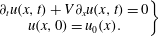 $$\begin{eqnarray}\left.\begin{array}{@{}c@{}}\unicode[STIX]{x2202}_{t}u(x,t)+V\unicode[STIX]{x2202}_{x}u(x,t)=0\\ u(x,0)=u_{0}(x).\end{array}\right\}\end{eqnarray}$$
The solution has the form,
 $$\begin{eqnarray}u(x,t)=u_{0}(x-V\ast t).\end{eqnarray}$$
Moreover, to avoid problems linked to boundaries, e.g. wave reflection, a periodic box is considered in the
 $x$
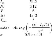
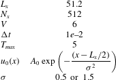
direction. The reference numerical set-up used for the simulations in this section is given in table 2.
Reference numerical set-up for the resolution of (5.1).
The same discretizations in space and time, as for the modelling of diffusion in the last section, are used here: CD in space and EE or IE in time, resulting in the following discrete equations,
 $$\begin{eqnarray}\displaystyle & \displaystyle \text{EE: }\frac{u_{i}^{n+1}-u_{i}^{n}}{\unicode[STIX]{x0394}t}=-V\frac{u_{i+1}^{n}-u_{i-1}^{n}}{2\unicode[STIX]{x0394}x}, & \displaystyle\end{eqnarray}$$
 $$\begin{eqnarray}\displaystyle & \displaystyle \text{IE: }\frac{u_{i}^{n+1}-u_{i}^{n}}{\unicode[STIX]{x0394}t}=-V\frac{u_{i+1}^{n+1}-u_{i-1}^{n+1}}{2\unicode[STIX]{x0394}x}. & \displaystyle\end{eqnarray}$$
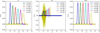
Numerical resolution of advection equation using CD in space for
 $\unicode[STIX]{x1D70E}=1.5$
with parameters:
 $N_{x}=512$
,
 $L_{x}=51.2$
and
 $\unicode[STIX]{x0394}t=1e{-}2$
.

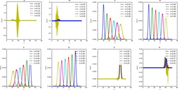
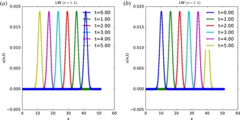
The results from the simulation of advection using EE and IE algorithms are plotted on figure 16. The IE scheme reproduces almost correctly the advection process, except that the Gaussian function is not just advected but also damped. In the case presented here, the IE
 $+$
CD scheme is stable but, in contrast to the resolution of the diffusion equation, this scheme is not unconditionally stable. The stability is linked to the values of
 $V,\unicode[STIX]{x0394}x$
and
 $\unicode[STIX]{x0394}t$
which must verify the inequality:
 $$\begin{eqnarray}0\leqslant V\frac{\unicode[STIX]{x0394}t}{\unicode[STIX]{x0394}x}\leqslant 1.\end{eqnarray}$$
The number
 $\unicode[STIX]{x1D707}=V\unicode[STIX]{x0394}t/\unicode[STIX]{x0394}x$
corresponds to the Courant number for advection. It has to be noticed that full agreement between the CFL condition and stability analysis is quite rare. As for the diffusion, the CFL condition is necessary but not sufficient to ensure stability (see Ferszinger Reference Ferszinger2002; Schneider et al.
Reference Schneider, Kolomenskiy and Deriaz2013). Details on the derivation of the CFL condition for the advection equation can be found for example in Leveque (Reference Leveque1992), Ferszinger (Reference Ferszinger2002). However, the EE is unstable even if simulations are performed with a value of
 $\unicode[STIX]{x1D707}<0.5$
. This unstable evolution is characterized here by an increase of the amplitude of the field (which is inconsistent with a pure advection process) and also, the growth of spurious oscillations at the queue of the profile can be noticed. These oscillations dominate in amplitude and overcome the expected profile. Unlike for diffusion, EE
 $+$
CD is unconditionally unstable which means that this scheme is unstable for any values of the parameters. This is verified by the same stability analysis using Von Neumann’s technique for the derivation of the amplification factor
 $G$
,
 $$\begin{eqnarray}\displaystyle & \displaystyle G(k)=1-\text{i}V\frac{\unicode[STIX]{x0394}t}{\unicode[STIX]{x0394}x}\sin (k\unicode[STIX]{x0394}x) & \displaystyle\end{eqnarray}$$
 $$\begin{eqnarray}\displaystyle & \displaystyle |G(k)|^{2}=1+V^{2}\frac{\unicode[STIX]{x0394}t^{2}}{\unicode[STIX]{x0394}x^{2}}\sin ^{2}(k\unicode[STIX]{x0394}x)\geqslant 1. & \displaystyle\end{eqnarray}$$
The source of the numerical instability is not the order of the spatial differentiation but the combination of spatial and temporal schemes used. Making the assumption that the finite space derivative is computed with a very-high-order method, e.g. the spectral method, (5.2) becomes
 $$\begin{eqnarray}\unicode[STIX]{x2202}_{t}u(x,t)+\text{i}k_{x}Vu(x,t)=0,\end{eqnarray}$$
and the amplification factor
 $G(k)$
becomes,
 $$\begin{eqnarray}\displaystyle & G(k)=1+\text{i}V\unicode[STIX]{x0394}t & \displaystyle\end{eqnarray}$$
 $$\begin{eqnarray}\displaystyle & |G(k)|^{2}=1+V^{2}\unicode[STIX]{x0394}t^{2}k_{x}^{2}\geqslant 1. & \displaystyle\end{eqnarray}$$
With an amplification factor always larger than 1 even using a spectral method, the EE scheme cannot be implemented correctly with any CD scheme in space. Time schemes other than Euler methods, such as e.g. Runge–Kutta methods are multistep and so Von Neumann’s stability analysis is not well suited. A stability analysis can be made using the notion of absolute stability (see Butcher Reference Butcher2008; Griffiths Reference Griffiths2010). Starting from a PDE of the form
 $\unicode[STIX]{x2202}_{t}u(x,t)=\unicode[STIX]{x1D706}u(x,t)$
with
 $\unicode[STIX]{x1D706}\in \mathbb{C}$
,
 $\unicode[STIX]{x1D706}$
represents any possible eigenvalue of the associated discrete system, and assuming that the solution has the form
 $$\begin{eqnarray}u^{n+1}=F(\unicode[STIX]{x1D706})u^{n},\end{eqnarray}$$
the scheme is stable if and only if
 $|F(\unicode[STIX]{x1D706})|\leqslant 1$
. As example, considering the EE scheme,
 $F$
is derived in 2 steps,
 $$\begin{eqnarray}\displaystyle \unicode[STIX]{x2202}_{t}u(t) & = & \displaystyle \unicode[STIX]{x1D706}u(t)\end{eqnarray}$$
 $$\begin{eqnarray}\displaystyle \Rightarrow u^{n+1} & = & \displaystyle (1+\unicode[STIX]{x1D706}\unicode[STIX]{x0394}t)u^{n}\end{eqnarray}$$
 $$\begin{eqnarray}\displaystyle \leftrightarrow F(\unicode[STIX]{x1D706}) & = & \displaystyle (1+\unicode[STIX]{x1D706}\unicode[STIX]{x0394}t).\end{eqnarray}$$
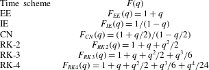
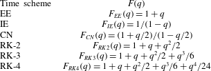
For the other time schemes presented here, posing
 $q=\unicode[STIX]{x1D706}\unicode[STIX]{x0394}t$
, the function
 $F(q)$
is given in table 3.
Analytic expression for function
 $F(q)$
.
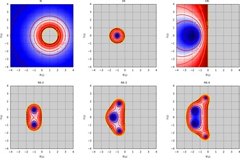
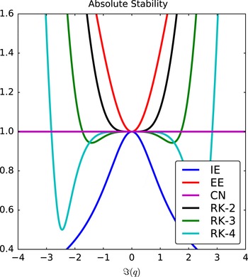
Corresponding stability diagrams of these time schemes are presented in figure 19. From these diagrams, the reasons why RK schemes are so widely used appear more clearly. Compared to Euler schemes, RK algorithms are of higher order and also their stability region increases with the scheme order (e.g. the stability region is wider than the one associated with the CFL condition). The width of the associated stability region is also a huge benefit compared with typical multistep methods for which the stable region shrinks with the scheme order (see Butcher Reference Butcher2008). In the simple case of advection at constant velocity and considering first- or second-order discretizations in space,
 $F(\unicode[STIX]{x1D706})$
values can be calculated literally. With a space discretization on
 $M$
mesh points let us start from the general expression of a first- or second-order space derivative,
 $$\begin{eqnarray}\unicode[STIX]{x2202}_{x}u_{i}=(au_{i-1}+bu_{i}+cu_{i+1})/\unicode[STIX]{x0394}x.\end{eqnarray}$$
Inserting (5.15) in (5.1) and using EE for the time discretization, a linear algebraic system is obtained,
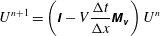 $$\begin{eqnarray}U^{n+1}=\left(\unicode[STIX]{x1D644}-V\frac{\unicode[STIX]{x0394}t}{\unicode[STIX]{x0394}x}\unicode[STIX]{x1D648}_{\unicode[STIX]{x1D66B}}\right)U^{n}\end{eqnarray}$$
with
 $\unicode[STIX]{x1D644}$
representing the identity matrix,
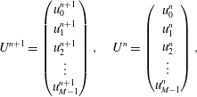 $$\begin{eqnarray}U^{n+1}=\left(\begin{array}{@{}c@{}}u_{0}^{n+1}\\ u_{1}^{n+1}\\ u_{2}^{n+1}\\ \vdots \\ u_{M-1}^{n+1}\end{array}\right),\quad U^{n}=\left(\begin{array}{@{}c@{}}u_{0}^{n}\\ u_{1}^{n}\\ u_{2}^{n}\\ \vdots \\ u_{M-1}^{n}\end{array}\right),\end{eqnarray}$$
and
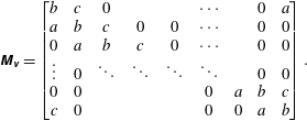 $$\begin{eqnarray}\unicode[STIX]{x1D648}_{\unicode[STIX]{x1D66B}}=\left[\begin{array}{@{}ccccccccc@{}}b & c & 0 & & & \cdots \, & & 0 & a\\ a & b & c & 0 & 0 & \cdots \, & & 0 & 0\\ 0 & a & b & c & 0 & \cdots \, & & 0 & 0\\ \vdots & 0 & \ddots & \ddots & \ddots & \ddots & & 0 & 0\\ 0 & 0 & & & & 0 & a & b & c\\ c & 0 & & & & 0 & 0 & a & b\end{array}\right].\end{eqnarray}$$
The matrix
 $\unicode[STIX]{x1D648}_{\unicode[STIX]{x1D66B}}$
belongs to the class of circulant Toeplitz matrices. A matrix is said to be Toeplitz if it is a diagonal constant matrix, which means that all the elements along a diagonal have the same constant value. Eigenvalues (and eigenfunctions) of such kinds of matrices can be easily calculated analytically (see Smith Reference Smith1978) and in the tridiagonal case, the eigenvalues of
 $\unicode[STIX]{x1D648}_{\unicode[STIX]{x1D66B}}$
are expressed by (demonstration in appendix B, (B 10)):
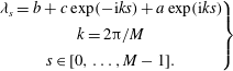 $$\begin{eqnarray}\left.\begin{array}{@{}c@{}}\unicode[STIX]{x1D706}_{s}=b+c\exp (-\text{i}ks)+a\exp (\text{i}ks)\\ k=2\unicode[STIX]{x03C0}/M\\ s\in [0,\ldots ,M-1].\end{array}\right\}\end{eqnarray}$$
The system (5.16) becomes,
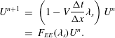 $$\begin{eqnarray}\displaystyle U^{n+1} & = & \displaystyle \left(1-V\frac{\unicode[STIX]{x0394}t}{\unicode[STIX]{x0394}x}\unicode[STIX]{x1D706}_{s}\right)U^{n}\nonumber\\ \displaystyle & = & \displaystyle F_{EE}(\unicode[STIX]{x1D706}_{s})U^{n}.\end{eqnarray}$$
In the case of CD discretization,
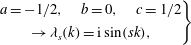 $$\begin{eqnarray}\displaystyle \left.\begin{array}{@{}c@{}}a=-1/2,\quad b=0,\quad c=1/2\\ \rightarrow \unicode[STIX]{x1D706}_{s}(k)=\text{i}\sin (sk),\end{array}\right\} & & \displaystyle\end{eqnarray}$$
inserting into (5.20),
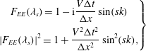 $$\begin{eqnarray}\displaystyle \left.\begin{array}{@{}c@{}}\displaystyle F_{EE}(\unicode[STIX]{x1D706}_{s})=1-\text{i}\frac{V\unicode[STIX]{x0394}t}{\unicode[STIX]{x0394}x}\sin (sk)\\ \displaystyle |F_{EE}(\unicode[STIX]{x1D706}_{s})|^{2}=1+\frac{V^{2}\unicode[STIX]{x0394}t^{2}}{\unicode[STIX]{x0394}x^{2}}\sin ^{2}(sk),\end{array}\right\} & & \displaystyle\end{eqnarray}$$
which confirms the unstable characteristic of this scheme in that case, since
 $|F_{EE}(\unicode[STIX]{x1D706}_{s})|\geqslant 1$
. More precisely, for any symmetric discretization,
 $\unicode[STIX]{x1D706}_{s}$
(and
 $q$
) is purely imaginary, so in any case,
 $|F(q)|\geqslant 1$
. As illustrated in figure 20, EE and RK-2 schemes are unconditionally unstable for advection using central spatial derivatives.
Since the CD scheme is unconditionally unstable, the next step is to look at other possible spatial discretizations, FWD and BWD discretizations. BWD leads to the following values for
 $a,b$
and
 $c$
,
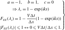 $$\begin{eqnarray}\displaystyle \left.\begin{array}{@{}c@{}}a=-1,\quad b=1,\quad c=0\\ \Rightarrow \unicode[STIX]{x1D706}_{s}=1-\exp (\text{i}ks)\\ \displaystyle F_{EE}(\unicode[STIX]{x1D706}_{s})=1-\frac{V\unicode[STIX]{x0394}t}{\unicode[STIX]{x0394}x}(1-\exp (\text{i}ks))\\ |F_{EE}(\unicode[STIX]{x1D706}_{s})|\leqslant 1\leftrightarrow 0\leqslant V\unicode[STIX]{x0394}t/\unicode[STIX]{x0394}x\leqslant 1.\end{array}\right\} & & \displaystyle\end{eqnarray}$$
The BWD scheme is stable if
 $0\leqslant V\unicode[STIX]{x0394}t/\unicode[STIX]{x0394}x\leqslant 1$
. It has to be noticed that, the coefficient
 $V$
which represents the advection velocity can be positive or negative, depending on the direction of the flow. As a consequence, if the direction is from right to left,
 $V$
is negative and therefore BWD becomes unstable.
Assuming
 $V<0$
, the last possibility is not to use BWD but FWD scheme. The associated coefficients are,
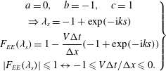 $$\begin{eqnarray}\displaystyle \left.\begin{array}{@{}c@{}}a=0,\quad b=-1,\quad c=1\\ \Rightarrow \unicode[STIX]{x1D706}_{s}=-1+\exp (-\text{i}ks)\\ \displaystyle F_{EE}(\unicode[STIX]{x1D706}_{s})=1-\frac{V\unicode[STIX]{x0394}t}{\unicode[STIX]{x0394}x}(-1+\exp (-\text{i}ks))\\ |F_{EE}(\unicode[STIX]{x1D706}_{s})|\leqslant 1\leftrightarrow -1\leqslant V\unicode[STIX]{x0394}t/\unicode[STIX]{x0394}x\leqslant 0.\end{array}\right\} & & \displaystyle\end{eqnarray}$$
The stability condition is ‘symmetric’ to the one for
 $V>0$
in the BWD case, i.e. for
 $V<0$
:
 $-1\leqslant V\unicode[STIX]{x0394}t/\unicode[STIX]{x0394}x\leqslant 0$
. This class of methods, for which spatial discretization is skewed in the direction from which the flow comes from is called ‘upwind’ method. The origin of upwind methods can be traced back to the initial work of (see Courant, Isaacson & Rees Reference Courant, Isaacson and Rees1952). The link between stability and the direction of the flow is illustrated in figure 17. When the flow comes from the left (
 $V>0$
), only BWD are stable. At the opposite, when the flow came from the right (
 $V<0$
), only FWD are stable, as expected from the stability analysis.
Influence on flow direction (
 $V=-6$
on top and
 $V=6$
on bottom) on implicit and explicit time schemes (IE and EE) with, forward/backward spatial derivative.

The last property which can be noticed for advection process simulations is that, even if the scheme is stable, the solution is damped. This dissipation phenomenon observed for the EE scheme is directly linked to the truncation error of the method. In fact, the equation solved numerically is, assuming FD in space (see Leveque Reference Leveque1992),
 $$\begin{eqnarray}\unicode[STIX]{x2202}_{t}u(x,t)+V\unicode[STIX]{x2202}_{x}u(x,t)-\frac{V}{2}(\unicode[STIX]{x0394}x-V\unicode[STIX]{x0394}t)\unicode[STIX]{x2202}_{x}^{2}u(x,t)=0.\end{eqnarray}$$
The dissipative damping generated is directly linked to the discretization steps.
In § 4, the advantage of implicit schemes has been demonstrated for the diffusion operator. In particular, time steps can be larger than the one allowed by the CFL condition. However, in hyperbolic systems, implicit methods require more computational work per time step compared to explicit methods. This is linked to the mathematical properties of the associated matrix. Moreover, due to truncation errors, the solutions obtained with larger time steps are less accurate (see Jardin Reference Jardin2011). The presented schemes are only first order in space, since the unstable character of the CD derivative has been demonstrated. It can be interesting to develop a scheme which is stable and second order in space. This method can be derived using analysis of the truncation error, in the case where CD derivatives are used. The equation which is resolved in fact is the following one,
 $$\begin{eqnarray}\displaystyle & \displaystyle \unicode[STIX]{x2202}_{t}u(x,t)+V\unicode[STIX]{x2202}_{x}u(x,t)=-D\unicode[STIX]{x2202}_{x}^{2}u(x,t) & \displaystyle\end{eqnarray}$$
 $$\begin{eqnarray}\displaystyle & \displaystyle D=\frac{V^{2}}{2}\unicode[STIX]{x0394}t. & \displaystyle\end{eqnarray}$$
As a consequence, if CD derivatives are implemented, adding an artificial diffusion with a coefficient
 $D^{\prime }=(V^{2}/2)\unicode[STIX]{x0394}t$
leads to a cancellation of this anormal diffusion and the scheme becomes stable. This procedure is known as the Lax–Wendroff (LW) differential scheme and permits the resolution of advection with second-order derivatives in space (see Lax & Wendroff Reference Lax and Wendroff1960) and increased stability in time to order 3. The interest of LW is confirmed in figure 18 where (5.2) is resolved successfully using CD in space. Implementation of CD in space allows to use the same discretization independently of the flow direction. Since the amplitude remains constant in time, the LW scheme, as with RK-4, is non-dissipative, opposite to the Euler schemes.
Advection using LW scheme with
 $V=-6$
(a) and
 $V=6$
(b).

The non-dissipative property of this scheme is really interesting to obtain an accurate solution. This property is not the only one necessary to obtain a realistic solution, it is also necessary to check if the scheme is dispersive or not. The dispersion error can be seen as the difference between the physical propagation velocity and the numerical propagation velocity. The consequence is that a scheme suffering from dispersion leads to appearance of oscillations in the numerical solution. Both errors, dissipation and dispersion, can be analysed using the amplification factor derived from the stability analysis. The main assumption for the stability (and the accuracy) of a scheme concerns the modulus of the factor
 $G$
. This modulus gives the diffusion error of the scheme. If
 $|G|=1$
, the amplitude of the solution is not damped in time due to artificial diffusion. If
 $|G|\leqslant 1$
, the solution is damped but, at the same time, waves can develop at small scales due to numerical errors. Developing schemes with a better control of this damping leads to the existence of more accurate schemes which suppress the oscillations. As mentioned before, an example for the advection equation, the Lax method (see Leveque Reference Leveque2002) adds an artificial diffusion, with a diffusion coefficient derived from the truncation error of the scheme.
Stability diagram for IE, EE, CN, RK-2, RK-3 and RK-4 schemes using the absolute stability criterion. A scheme is stable if
 $|q|\leqslant 1$
which corresponds to the colour range from blue to red. Grey zones correspond to
 $|q|>1$
.

Slice of the absolute stability diagrams for IE, EE, CN, RK-2, RK-3 and RK-4 schemes corresponding to values of
 $q$
purely imaginary.

Oscillations occurring in the resolution of advection equation (
 $\unicode[STIX]{x1D70E}=0.5$
) for LW (b) and RK-4 (c) schemes.

Since
 $G$
is complex, additional information can be obtained using the expression of
 $G$
in polar form,
 $G=a+\text{i}b=|G|\text{e}^{\text{i}\unicode[STIX]{x1D703}}$
. The argument
 $\unicode[STIX]{x1D703}$
characterizes the phase speed error of the system (see Durran Reference Durran1999; Hirsch Reference Hirsch2007). The dispersion error (
 $\unicode[STIX]{x1D716}_{\unicode[STIX]{x1D719}}$
) is expressed by the ratio between the physical phase speed of the considered equation and the numerical phase speed,
 $\unicode[STIX]{x1D703}$
. If
 $\unicode[STIX]{x1D716}_{\unicode[STIX]{x1D719}}>1$
, the numerical propagation is larger than the exact one and the computed solution appears to move faster than the real one. If
 $\unicode[STIX]{x1D716}_{\unicode[STIX]{x1D719}}<1$
, the numerical solution travels at a lower velocity than the physical one.
The numerical accuracy of a scheme is not only linked to these errors but also, in a more subtle way, to the main assumption concerning Taylor’s expansion in space. Finite differences are based on the interpolation of discrete data using polynomials (like Taylor’s series) or other simple functions. As a consequence, schemes of order
 $P$
can advect without error any polynomial of the same order. However, at a position close to a stiff gradient or discontinuity, the interpolation polynomial will not converge and oscillations will appear. Such oscillations, called Gibb’s oscillations, will not decay in magnitude when the mesh is refined. As an example, and to explain why more advanced schemes are used to resolve the advection process, the resolution of (5.2) is realized again using the same parameters for
 $V$
,
 $\unicode[STIX]{x0394}x$
,
 $\unicode[STIX]{x0394}t$
presented in figure 21. The only change is the width of the Gaussian (
 $\unicode[STIX]{x1D70E}$
) used as initial condition. In plasma fluid dynamics, the width of relevant modes are parameter dependent. For example, the width of the eigenfunctions corresponding to resistive ballooning modes depend on the mode number (see Beyer, Benkadda & Garbet Reference Beyer, Benkadda and Garbet2000),
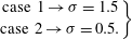 $$\begin{eqnarray}\displaystyle \left.\begin{array}{@{}c@{}}\text{case 1}\rightarrow \unicode[STIX]{x1D70E}=1.5\\ \text{case 2}\rightarrow \unicode[STIX]{x1D70E}=0.5.\end{array}\right\} & & \displaystyle\end{eqnarray}$$
Since the discretization parameters remain the same, a change in the initial profile does not affect the CFL condition. However the RK scheme becomes dissipative and spurious oscillations appear. This behaviour cannot be suppressed switching from central differences for the space derivatives to forward derivatives at the same order. To control and try to avoid this effect, more advanced (higher-order) schemes have been developed. The main hypothesis is that since advection is a conservative process, the algorithm should be formulated to conserve the advected quantity numerically. This formulation is a numerically flux conserving form. Using the Godunov theorem which says that any linear algorithm for solving partial differential equations, with the property of not producing new extrema can be at most first order, there is therefore no hope of finding a linear second-order accurate scheme that does not produce these unwanted oscillations. More advanced nonlinear schemes that combine the higher-order accuracy and the prevention of producing unwanted oscillations can be classified into two categories (see Leveque Reference Leveque1992):
-
(i) flux-splitting methods (see Boris & Book Reference Boris and Book1997): artificial viscosity, relaxation schemes or methods based on the application of a limiter to eliminate the oscillations: total variation diminishing (TVD);
-
(ii) Godunov method (see Godunov Reference Godunov1959): monotonic upwind-centred scheme for conservation laws (MUSCL) scheme, piecewise parabolic method (PPM), essential non-oscillatory (ENO).
In the following, this last method (ENO) is briefly described and an improved version, the weighty essential non-oscillatory (WENO) method is also mentioned (see Shu Reference Shu1998). As for most advanced schemes for advection, the basic idea is to express the hyperbolic equation as a conservation law
 $$\begin{eqnarray}\unicode[STIX]{x2202}_{t}u(x,t)+\unicode[STIX]{x2202}_{x}[f(u(x,t))]=0.\end{eqnarray}$$
As a consequence, the discrete equation can be expressed as,
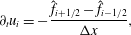 $$\begin{eqnarray}\unicode[STIX]{x2202}_{t}u_{i}=-\frac{\hat{f}_{i+1/2}-\hat{f}_{i-1/2}}{\unicode[STIX]{x0394}x},\end{eqnarray}$$
where
 $\hat{f}$
corresponds to a high-order approximation of the numerical flux. The notation
 $\text{i}+1/2$
signifies an estimation of the flux at the interface between two virtual cells of centre
 $i$
and
 $i+1$
.
Numerical resolution of advection equation for
 $\unicode[STIX]{x1D70E}=0.5$
with WENO scheme and parameters:
 $N_{x}=512,L_{x}=51.2$
, and
 $\unicode[STIX]{x0394}t=1e{-}2$
.

The key idea in ENO schemes to bypass the limitations given by Godunov’s theorem is to use an adaptive stencil procedure that results in a non-oscillatory nonlinear interpolation across discontinuities. The weighted essentially non-oscillatory (WENO) scheme is an improvement over the ENO schemes by replacing the stencil selection by a weighted average of the candidate stencils. Smoothness-dependent weights are used such that they approach zero for candidate stencils with discontinuities. Thus, across discontinuities, the WENO schemes behave like the ENO schemes, while in smooth regions of the solution, the weighted average results in a higher-order approximation. An alternative of the WENO scheme has been realized by Suresh and Huyn. This scheme is well adapted for RK time stepping and is accurate and faster than the corresponding fifth-order WENO scheme (see Suresh & Huynh Reference Suresh and Huynh1997). Figure 22 shows that the higher-order schemes exhibit higher accuracy and the quantity is transported without strong deterioration of the shape. It has to be noticed that only the fifth order is considered here and not the lower-order algorithms (such as third) because these schemes are too dissipative to be considered as accurate. The classical fifth-order WENO has also a dissipative component which is not discussed in detail here. As a consequence, for an accurate resolution of a pure advection problem, an adapted version using an anti-diffusive flux correction technique can be implemented, see Zhengfu & Shu (Reference Zhengfu and Shu2005) for details.
6 Nonlinear phenomena: the Poisson bracket
Nonlinear operators in fluid descriptions of plasmas are often expressed by Poisson brackets (Jacobian operator, noted
 $J(\unicode[STIX]{x1D701},\unicode[STIX]{x1D713})$
) between two quantities. The Jacobian is expressed as follows in Cartesian coordinates,
 $$\begin{eqnarray}J(\unicode[STIX]{x1D701},\unicode[STIX]{x1D713})=\unicode[STIX]{x2202}_{x}\unicode[STIX]{x1D701}(x,y)\unicode[STIX]{x2202}_{y}\unicode[STIX]{x1D713}(x,y)-\unicode[STIX]{x2202}_{x}\unicode[STIX]{x1D713}(x,y)\unicode[STIX]{x2202}_{y}\unicode[STIX]{x1D701}(x,y).\end{eqnarray}$$
The numerical resolution of the Jacobian operator has to be treated carefully. Since nonlinear coupling can drive and dominate energy cascade phenomena and, as a consequence, modifications of the equilibrium or generation of small-scale turbulence may appear, avoiding numerical instabilities or errors (for example truncation errors linked to FD schemes) is important to obtain accurate simulations and results. Compared to linear advection, the computation of the Jacobian is really more expensive. As a consequence using an optimized and accurate method can greatly reduce necessary CPU time for a simulation. Possible algorithms are chosen mainly using geometry properties of the considered system. For fusion plasma simulations, periodicity properties of the tokamak permit to use a Fourier mode decomposition for toroidal and (quite often) poloidal directions. As mentioned previously, (see Canuto et al.
Reference Canuto, Hussaini, Quarteroni and Zang1988; Ferszinger Reference Ferszinger2002), spectral methods are more accurate than any FD scheme. Also, the precision order for calculations of any derivative is higher using Fourier mode decomposition. The accuracy of the calculation of a derivative in real space is determined by the precision order of the considered formula, (
 $O(\unicode[STIX]{x0394}x),O(\unicode[STIX]{x0394}x^{2}),\ldots$
). In Fourier space, the same accuracy is obtained using only a few modes, it can be considered for example that the calculation with
 $1$
mode corresponds to a precision of
 $O(\unicode[STIX]{x0394}x)$
, 2 modes of
 $O(\unicode[STIX]{x0394}x^{2})$
and so on.
Using this representation, the resolution of the Jacobian operator in semi spectral space (FD representation in
 $x$
and spectral representation in
 $y$
in a 2-D slab geometry) is equivalent to the computation of two discrete convolutions, the associated complexity is of order
 $M^{2}$
with
 $M$
being the number of modes. However, if the Jacobian is computed in real space, the complexity is of the order
 $M$
only, which is a benefit with increasing
 $M$
. Since the fields are stored in a semispectral way, the computation of the discrete Fourier transform (FT) of
 $\unicode[STIX]{x1D701}$
and
 $\unicode[STIX]{x1D713}$
must be made first, then calculate the Jacobian in real space, and finally compute an inverse transform (IFT). This method requires more intermediate steps than the direct calculation, but the complexity scales only as
 $M\ast (2\ast \log (M)+1)$
. To give an idea of the associated number of operations to perform, if
 $M=16$
, the Fourier method is
 $\simeq 2.5\times$
faster, if
 $M=128$
, the Fourier method is
 $\simeq 10\times$
faster. In the 3-D case, using spectral representation with
 $M$
poloidal and
 $N$
toroidal modes, the number of operations scales like
 $N^{2}\ast M^{2}$
for the direct product and like
 $N\ast M\ast (2\ast \log (N\ast M)+1)$
for the Fourier method. As a consequence, the resolution in real space, even with the constraint on the necessary Fourier transforms, is more effective. However, this resolution procedure shadows caveats which can lead to numerical instabilities detailed in the following subsections,
-
(i) consequences of direct and inverse FT;
-
(ii) accurate calculation of Jacobian.
6.1 Fourier transformation
In computational sciences, the FT corresponds to the discrete Fourier series. As a consequence, the phenomenon of aliasing could appear in the process. Considering a Fourier mode
 $\text{e}^{\text{i}\boldsymbol{k}_{l}x_{j}}$
with
 $\boldsymbol{k}_{l}$
the wave vector and
 $x_{j}$
the grid point.
 $$\begin{eqnarray}\displaystyle & \displaystyle \boldsymbol{k}_{l}=2\unicode[STIX]{x03C0}l/(N\ast \unicode[STIX]{x0394}x),\quad l=-N/2,\ldots ,N/2 & \displaystyle\end{eqnarray}$$
 $$\begin{eqnarray}\displaystyle & \displaystyle x_{j}=j\unicode[STIX]{x0394}x,\quad j=0,1,\ldots ,N. & \displaystyle\end{eqnarray}$$
At the grid point
 $x_{j}$
, the following relation holds
 $$\begin{eqnarray}\text{e}^{\text{i}2\unicode[STIX]{x03C0}(j+l\ast N)p/N}=\text{e}^{\text{i}2\unicode[STIX]{x03C0}j/N},\quad p=\ldots ,-2,-1,0,1,2,\ldots .\end{eqnarray}$$
As a consequence, the modes
 $k_{j}=2\unicode[STIX]{x03C0}j/(N\ast \unicode[STIX]{x0394}x)$
contribute to the discrete FT but, and this is the reason for possible numerical errors, the mode
 $k_{p}=2\unicode[STIX]{x03C0}(j+p\ast N)/(N\ast \unicode[STIX]{x0394}x)$
also. High-
 $k$
modes smear out the amplitude of a lower-
 $k$
mode. This can cause, for example, an increase of the energy of the system. To prevent this aliasing phenomena, several methods have been developed (see Patterson & Orszag Reference Patterson and Orszag1971), e.g. performing a phase-shifted transform. However, the bottleneck is that the correct transform needs the calculation of eight Fourier transforms each time. The most widely used method is the following one, which can be achieved by enlarging each dimension of the spectral domain by a factor of
 $(M+1)/2$
where
 $M$
is the number of modes. An alternative consist to use
 $2/3$
of the modes for the Fourier transform, this method is generally called the ‘
 $2/3$
rule’. In general the de-aliasing rule is applied not by an increase of
 $3/2$
of the number of mode but by an increase to the next power of 2. This is because an optimized algorithm for FT exists when the size is a power of 2, named fast Fourier transform (FFT) method. This algorithm has highly increased performance compared to the approach based on the mathematical definition (see Press et al.
Reference Press, Teukolsky, Vetterling and Flannery2007). In that case, number of necessary operations scales as
 $N\log (N)$
and not as
 $N^{2}$
for the 1-D case.
6.2 Accurate Jacobian
An accurate value of the Jacobian needs a clever differentiating formulation. The Jacobian is mainly a product of derivatives in the
 $x$
and
 $y$
directions. Apparently, a second-order FD based on central differences can be implemented,
 $$\begin{eqnarray}J(\unicode[STIX]{x1D701},\unicode[STIX]{x1D713})=\frac{1}{4\unicode[STIX]{x0394}x\unicode[STIX]{x0394}y}((\unicode[STIX]{x1D701}_{i+1,j}-\unicode[STIX]{x1D701}_{i-1,j})\ast (\unicode[STIX]{x1D713}_{i,j+1}-\unicode[STIX]{x1D713}_{i,j-1})-(\unicode[STIX]{x1D701}_{i,j+1}-\unicode[STIX]{x1D701}_{i,j-1})\ast (\unicode[STIX]{x1D713}_{i+1,j}-\unicode[STIX]{x1D713}_{i-1,j})).\end{eqnarray}$$
As an example, a 2-D mesh is used, and the functions
 $\unicode[STIX]{x1D701}$
and
 $\unicode[STIX]{x1D713}$
are defined by,
 $$\begin{eqnarray}\displaystyle & \unicode[STIX]{x1D701}(x,y)=\text{e}^{-((x-x_{0})^{2}+(y-y_{0})^{2})}+\text{e}^{-((x+x_{0})^{2}+(y+y_{0})^{2})} & \displaystyle\end{eqnarray}$$
 $$\begin{eqnarray}\displaystyle & \unicode[STIX]{x1D713}(x,y)=\unicode[STIX]{x2202}_{x}^{2}\unicode[STIX]{x1D701}(x,y)+\unicode[STIX]{x2202}_{y}^{2}\unicode[STIX]{x1D701}(x,y). & \displaystyle\end{eqnarray}$$
The analytic values of
 $\unicode[STIX]{x1D713}$
and the associated Jacobian have been analytically calculated and discretized on the same grid to avoid errors associated with any FD scheme (corresponding plots are represented on figure 23).
Representation of input functions
 $\unicode[STIX]{x1D701}$
,
 $\unicode[STIX]{x1D713}$
and calculated Jacobian (
 $J$
) for a mesh size of
 $512\times 512$
points.

Computed Jacobian with CD (a,c) and Arakawa (b,d) methods for two grid sizes,
 $64\times 64$
and
 $256\times 256$
.

 $R^{2}$
value with respect to exact value of the Jacobian for the 2 schemes, Arakawa and CD.

Arakawa stencils used to ensure conservation of enstrophy and kinetic energy.

The Jacobian obtained through a simple product of centre derivatives is plotted in figure 24(a,c) for two mesh sizes:
 $64\times 64$
and
 $256\times 256$
points, respectively. Comparing to the exact solution (figure 23
c), the CD method produces inconsistent results due to irrelevant extrema at low resolutions. The amplitudes of these spurious extrema are damped when the resolution is increased but they are still present with a resolution of
 $256\times 256$
points. Using statistical tools, and more precisely the coefficient of determination
 $R^{2}$
, a convergence rate to the analytical solution can be expressed as a function of the mesh resolution. The results are plotted on figure 25. It appears that the solution converges to the analytical one when the number of points (and as a consequence the associated precision) increases. However, this convergence requires a large number of points.
Products based on central schemes raise another issue which is more relevant for longer term simulations. Platzmann (see Platzman Reference Platzman1961) has shown that the product of CD leads to the appearance of small eddies which will usually intensify causing computational instability or at least a numerical source of energy in the system. These eddies, also known as ‘noodling’ in the literature have been observed in plasma fluid simulations (see Brock & Horton Reference Brock and Horton1982) and they are linked to another aliasing error source which is inherent to FD schemes: a FD scheme is not able to treat correctly waves with wavenumbers smaller than
 $\unicode[STIX]{x0394}x/2$
. A typical consequence is an unexplained growth of the kinetic energy of the system. A more robust scheme for long term simulations which overcomes this computational instability has been developed by Arakawa (see Arakawa Reference Arakawa1966). This scheme ensures conservation of energy and enstrophy under the action of the Jacobian. The main idea is to calculate an average between products using central derivatives (called
 $J1$
) and two other alternative formulas which ensure enstrophy conservation (
 $J2$
) and energy conservation
 $J3$
, figure 26.
 $$\begin{eqnarray}\displaystyle J_{1} & = & \displaystyle \unicode[STIX]{x2202}_{x}\unicode[STIX]{x1D701}\unicode[STIX]{x2202}_{y}\unicode[STIX]{x1D713}-\unicode[STIX]{x2202}_{y}\unicode[STIX]{x1D701}\unicode[STIX]{x2202}_{x}\unicode[STIX]{x1D713}\end{eqnarray}$$
 $$\begin{eqnarray}\displaystyle J_{2} & = & \displaystyle -\unicode[STIX]{x2202}_{x}(\unicode[STIX]{x1D713}\unicode[STIX]{x2202}_{y}\unicode[STIX]{x1D701})+\unicode[STIX]{x2202}_{y}(\unicode[STIX]{x1D713}\unicode[STIX]{x2202}_{x}\unicode[STIX]{x1D701})\end{eqnarray}$$
 $$\begin{eqnarray}\displaystyle J_{3} & = & \displaystyle \unicode[STIX]{x2202}_{x}(\unicode[STIX]{x1D701}\unicode[STIX]{x2202}_{y}\unicode[STIX]{x1D713})-\unicode[STIX]{x2202}_{y}(\unicode[STIX]{x1D701}\unicode[STIX]{x2202}_{x}\unicode[STIX]{x1D713})\end{eqnarray}$$
 $$\begin{eqnarray}\displaystyle \Rightarrow J(\unicode[STIX]{x1D701},\unicode[STIX]{x1D713}) & = & \displaystyle (J_{1}+J_{2}+J_{3})/3.\end{eqnarray}$$
The procedure can be described as an advanced use of the method of undetermined coefficients for a nine-point stencil for functions
 $\unicode[STIX]{x1D713}$
and
 $\unicode[STIX]{x1D701}$
,
 $$\begin{eqnarray}J_{i,j}(\unicode[STIX]{x1D701},\unicode[STIX]{x1D713})=\mathop{\sum }_{i^{\prime }=-1}^{1}\mathop{\sum }_{j^{\prime }=-1}^{1}\mathop{\sum }_{i^{\prime \prime }=-1}^{1}\mathop{\sum }_{j^{\prime \prime }=-1}^{1}c_{i,j,i^{\prime },j^{\prime },i^{\prime \prime },j^{\prime \prime }}\unicode[STIX]{x1D701}_{i+i^{\prime },j+j^{\prime }}\unicode[STIX]{x1D713}_{i+i^{\prime \prime },j+j^{\prime \prime }}.\end{eqnarray}$$
The quantities
 $a_{i,j,i+i^{\prime },j+j^{\prime }}$
and
 $b_{i,j,i+i^{\prime \prime },j+j^{\prime \prime }}$
which will be used to simplify the final expressions, are defined as,
 $$\begin{eqnarray}\displaystyle & \displaystyle a_{i,j,i+i^{\prime },j+j^{\prime }}=\mathop{\sum }_{i^{\prime \prime }}\mathop{\sum }_{j^{\prime \prime }}c_{i,j,i^{\prime },j^{\prime },i^{\prime \prime },j^{\prime \prime }}\unicode[STIX]{x1D713}_{i+i^{\prime \prime },j+j^{\prime \prime }} & \displaystyle\end{eqnarray}$$
 $$\begin{eqnarray}\displaystyle & \displaystyle b_{i,j,i+i^{\prime \prime },j+j^{\prime \prime }}=\mathop{\sum }_{i^{\prime }}\mathop{\sum }_{j^{\prime }}c_{i,j,i^{\prime },j^{\prime },i^{\prime \prime },j^{\prime \prime }}\unicode[STIX]{x1D701}_{i+i^{\prime },j+j^{\prime }}. & \displaystyle\end{eqnarray}$$
The Jacobian is expressed by,
 $$\begin{eqnarray}\displaystyle J_{i,j}(\unicode[STIX]{x1D701},\unicode[STIX]{x1D713}) & = & \displaystyle \mathop{\sum }_{i^{\prime }}\mathop{\sum }_{j^{\prime }}a_{i,j,i+i^{\prime },j+j^{\prime }}\unicode[STIX]{x1D701}_{i+i^{\prime },j+j^{\prime }}\end{eqnarray}$$
 $$\begin{eqnarray}\displaystyle & = & \displaystyle \mathop{\sum }_{i^{\prime \prime }}\mathop{\sum }_{j^{\prime \prime }}b_{i,j,i+i^{\prime \prime },j+j^{\prime \prime }}\unicode[STIX]{x1D713}_{i+i^{\prime \prime },j+j^{\prime \prime }}.\end{eqnarray}$$
To verify the properties of the Jacobian and the energy conservation, the subsequent relations between coefficients are used (derivation can be found in Coiffier (Reference Coiffier2012)),
-
(i) skew-symmetric property,
$J_{i,j}(\unicode[STIX]{x1D701},\unicode[STIX]{x1D713})=-J_{i,j}(\unicode[STIX]{x1D713},\unicode[STIX]{x1D701})$
(6.17)
$$\begin{eqnarray}\displaystyle & & \displaystyle \mathop{\sum }_{i^{\prime }}\mathop{\sum }_{j^{\prime }}\mathop{\sum }_{i^{\prime \prime }}\mathop{\sum }_{j^{\prime \prime }}c_{i,j,i^{\prime },j^{\prime },i^{\prime \prime },j^{\prime \prime }}\unicode[STIX]{x1D701}_{i+i^{\prime },j+j^{\prime }}\unicode[STIX]{x1D713}_{i+i^{\prime \prime },j+j^{\prime \prime }}\nonumber\\ \displaystyle & & \displaystyle \quad =-\mathop{\sum }_{i^{\prime }}\mathop{\sum }_{j^{\prime }}\mathop{\sum }_{i^{\prime \prime }}\mathop{\sum }_{j^{\prime \prime }}c_{i,j,i^{\prime },j^{\prime },i^{\prime \prime },j^{\prime \prime }}\unicode[STIX]{x1D701}_{i+i^{\prime \prime },j+j^{\prime \prime }}\unicode[STIX]{x1D713}_{i+i^{\prime },j+j^{\prime }}\nonumber\\ \displaystyle & & \displaystyle \quad \Rightarrow c_{i,j,i^{\prime },j^{\prime },i^{\prime \prime },j^{\prime \prime }}=-c_{i,j,i^{\prime \prime },j^{\prime \prime },i^{\prime },j^{\prime }},\end{eqnarray}$$
-
(ii) conservation of enstrophy
$\int \;\text{dS}\,\unicode[STIX]{x1D701}J(\unicode[STIX]{x1D701},\unicode[STIX]{x1D713})=0$
(6.18)
$$\begin{eqnarray}\displaystyle & & \displaystyle \mathop{\sum }_{i}\mathop{\sum }_{j}\unicode[STIX]{x0394}x\unicode[STIX]{x0394}y\unicode[STIX]{x1D701}_{i,j}J_{i,j}(\unicode[STIX]{x1D701},\unicode[STIX]{x1D713})\nonumber\\ \displaystyle & & \displaystyle \quad =\mathop{\sum }_{i}\mathop{\sum }_{j}\mathop{\sum }_{i^{\prime }}\mathop{\sum }_{j^{\prime }}\unicode[STIX]{x0394}x\unicode[STIX]{x0394}ya_{i,j,i+i^{\prime },j+j^{\prime }}\unicode[STIX]{x1D701}_{i,j}\unicode[STIX]{x1D701}_{i+i^{\prime },j+j^{\prime }}\nonumber\\ \displaystyle & & \displaystyle \quad \Rightarrow a_{i+i^{\prime },j+j^{\prime },i,j}=-a_{i,j,i+i^{\prime },j+j^{\prime }},\end{eqnarray}$$
-
(iii) conservation of kinetic energy
$\int \text{dS}\unicode[STIX]{x1D713}J(\unicode[STIX]{x1D701},\unicode[STIX]{x1D713})=0$
(6.19)
$$\begin{eqnarray}\displaystyle & & \displaystyle \mathop{\sum }_{i}\mathop{\sum }_{j}\unicode[STIX]{x0394}x\unicode[STIX]{x0394}y\unicode[STIX]{x1D713}_{i,j}J_{i,j}(\unicode[STIX]{x1D701},\unicode[STIX]{x1D713})\nonumber\\ \displaystyle & & \displaystyle \quad =\mathop{\sum }_{i}\mathop{\sum }_{j}\mathop{\sum }_{i^{\prime \prime }}\mathop{\sum }_{j^{\prime \prime }}\unicode[STIX]{x0394}x\unicode[STIX]{x0394}yb_{i,j,i+i^{\prime \prime },j+j^{\prime \prime }}\unicode[STIX]{x1D713}_{i,j}\unicode[STIX]{x1D713}_{i+i^{\prime \prime },j+j^{\prime \prime }}\nonumber\\ \displaystyle & & \displaystyle \quad \Rightarrow b_{i+i^{\prime \prime },j+j^{\prime \prime },i,j}=-b_{i,j,i+i^{\prime \prime },j+j^{\prime \prime }}.\end{eqnarray}$$

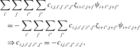

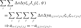

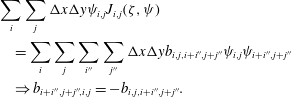
These three properties lead to the final formula for the discrete Jacobian,
 $$\begin{eqnarray}\displaystyle J(\unicode[STIX]{x1D701},\unicode[STIX]{x1D713}) & = & \displaystyle \frac{-1}{12\unicode[STIX]{x0394}x\unicode[STIX]{x0394}y} [(\unicode[STIX]{x1D713}_{i,j-1}+\unicode[STIX]{x1D713}_{i+1,j-1}-\unicode[STIX]{x1D713}_{i,j+1}-\unicode[STIX]{x1D713}_{i+1,j+1})\ast \unicode[STIX]{x1D701}_{i+1,j}\end{eqnarray}$$
 $$\begin{eqnarray}\displaystyle & & \displaystyle -\,(\unicode[STIX]{x1D713}_{i-1,j-1}+\unicode[STIX]{x1D713}_{i,j-1}-\unicode[STIX]{x1D713}_{i-1,j+1}-\unicode[STIX]{x1D713}_{i,j+1})\ast \unicode[STIX]{x1D701}_{i-1,j}\end{eqnarray}$$
 $$\begin{eqnarray}\displaystyle & & \displaystyle +\,(\unicode[STIX]{x1D713}_{i+1,j}+\unicode[STIX]{x1D713}_{i+1,j+1}-\unicode[STIX]{x1D713}_{i-1,j}-\unicode[STIX]{x1D713}_{i-1,j+1})\ast \unicode[STIX]{x1D701}_{i,j+1}\end{eqnarray}$$
 $$\begin{eqnarray}\displaystyle & & \displaystyle -\,(\unicode[STIX]{x1D713}_{i+1,j-1}+\unicode[STIX]{x1D713}_{i+1,j}-\unicode[STIX]{x1D713}_{i-1,j-1}-\unicode[STIX]{x1D713}_{i-1,j})\ast \unicode[STIX]{x1D701}_{i,j-1}\end{eqnarray}$$
 $$\begin{eqnarray}\displaystyle & & \displaystyle +\,(\unicode[STIX]{x1D713}_{i+1,j}-\unicode[STIX]{x1D713}_{i,j+1})\ast \unicode[STIX]{x1D701}_{i+1,j+1}\end{eqnarray}$$
 $$\begin{eqnarray}\displaystyle & & \displaystyle -\,(\unicode[STIX]{x1D713}_{i,j-1}-\unicode[STIX]{x1D713}_{i-1,j})\ast \unicode[STIX]{x1D701}_{i-1,j-1}\end{eqnarray}$$
 $$\begin{eqnarray}\displaystyle & & \displaystyle +\,(\unicode[STIX]{x1D713}_{i,j+1}-\unicode[STIX]{x1D713}_{i-1,j})\ast \unicode[STIX]{x1D701}_{i-1,j+1}\end{eqnarray}$$
 $$\begin{eqnarray}\displaystyle & & \displaystyle -\,(\unicode[STIX]{x1D713}_{i+1,j}-\unicode[STIX]{x1D713}_{i,j-1})\ast \unicode[STIX]{x1D701}_{i+1,j-1} ].\end{eqnarray}$$
This formulation is not the one given in the original paper (see Arakawa Reference Arakawa1966) but an optimized one (
 $\simeq 15\,\%$
faster) presented in Kuhn et al. (Reference Kuhn, Latu, Genaud and Crouseilles2013). Notice that in Kuhn et al. (Reference Kuhn, Latu, Genaud and Crouseilles2013), an optimized implementation of the full algorithm (FT
 $+$
Jacobian
 $+$
IFT) is presented and the resulting performance increase is approximately 75 % compared to a basic serial implementation. The results are plotted in figure 24(b,d). Compared to the CD scheme, the obtained Jacobian is more accurate. This is confirmed in figure 25 where the value of
 $R^{2}$
is plotted. Even with this simple example, the increased accuracy of the Arakawa scheme compared to a simple product of central differences is obvious. The increased accuracy is directly linked to the associated properties and not to the order since the implementation used is also second order as for the product of derivatives. A more detailed comparison of different schemes for the resolution of the Jacobian operator in PDEs has been made in Naulin & Nielsen (Reference Naulin and Nielsen2003).
7 Summary and discussion
Plasma fluid computations can be seen as a resolution of systems of partial differential equations. They therefore are subject to the main and principle difficulties linked to the resolution of such equations. The diversity of the physical processes involved in plasma physics leads to models implying a sum of mathematical operators. As a consequence, the associated numerical and mathematical limitations have to be treated carefully.
This paper focused on the main caveats that have to be avoided in plasma fluid simulations and on the algorithms permitting to avoid them. The numerical limitations are linked mainly to the presence of a finite grid and the correct treatment of small scales as well as wave propagation. An accurate treatment of small scales is necessary to study the role of turbulence on plasma dynamics and transport.
The increased performance of available super computers allows for the realization of simulations with higher resolutions for smaller spatial scales. As a consequence, the highest resolution simulations are closer to the experiments. For that purpose, numerical challenges which have not been presented in detail here lie in the matrix algebra and matrix inversion processes associated with the Poisson equation. The reason is linked to the mathematical nature of this equation, more precisely, the resolution of the Poisson equation at one grid point requires to gather data from the complete domain with the methods presented here. As a consequence, the communication due to the parallel resolution has a huge cost. More advanced methods/schemes can be used in that case, like the iterative approach, the conjugate gradient
 $\ldots$
(see Jardin Reference Jardin2010).
Considerable research and improvement over the past years have been accomplished also for the algorithms themselves. For that purpose, and in general, for all algebra linked to matrix inversions, resolution of linear systems, and matrix computations linked to implicit methods, specialized libraries developed should be used, e.g. MUMPS (2015), PasTiX (2015), SuperLU (2015). As cited in § 6, another time consuming computation which can be greatly reduced through the use of optimized algorithms and libraries is the computation of Fourier transforms, in that case a widely used library is the FFTW library (see FFTW 2015). During the development process, with the associated tests of methods, an alternative is to use a global framework for the resolution of PDEs like PETSc (see Balay et al. Reference Balay, Abhyankar, Adams, Brown, Brune, Buschelman, Dalcin, Eijkhout, Gropp and Kaushik2016).
Acknowledgements
The authors would like to thank W. Horton for helpful discussions and remarks on the manuscript. This work was granted access to the HPC resources of Aix-Marseille Université financed by the project Equip@Meso (ANR-10-EQPX-29-01) of the program ‘Investissements d’Avenir’ supervised by the Agence Nationale pour la Recherche.
Appendix A. List of abbreviations used
- AM
-
Adams–Moulton
- AB
-
Adams–Bashforth
- BWD
-
backward difference
- CD
-
central difference
- CFL
-
Courant–Friedrichs–Lewy
- CG
-
coarse graining
- CN
-
Crank–Nicholson
- EE
-
explicit Euler
- ENO
-
essentially non-oscillatory scheme
- FD
-
finite difference
- FT
-
Fourier transform
- FFT
-
fast Fourier transform
- FWD
-
forward difference
- IE
-
implicit Euler
- IFT
-
inverse Fourier transform
- LW
-
Lax–Wendroff scheme
- MPI
-
message passing interface
- PDE
-
partial differential equation
- RK
-
Runge–Kutta scheme
- WENO
-
weighted essentially non-oscillatory scheme
Appendix B. Eigenvalues and eigenfunctions of circulant matrices
In this appendix, the expression of eigenvalues for a periodic tridiagonal system is derived based on the derivation of eigenvalues of circulant matrices. Consider a circulant matrix
 $\unicode[STIX]{x1D63D}$
of size
 $M\times M\in \mathbb{R}^{2}$
of the form,
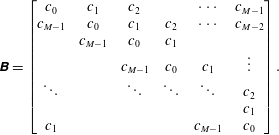 $$\begin{eqnarray}\unicode[STIX]{x1D63D}=\left[\begin{array}{@{}cccccc@{}}c_{0} & c_{1} & c_{2} & & \cdots \, & c_{M-1}\\ c_{M-1} & c_{0} & c_{1} & c_{2} & \cdots \, & c_{M-2}\\ & c_{M-1} & c_{0} & c_{1} & & \\ & & c_{M-1} & c_{0} & c_{1} & \vdots \\ \ddots & & \ddots & \ddots & \ddots & c_{2}\\ & & & & & c_{1}\\ c_{1} & & & & c_{M-1} & c_{0}\end{array}\right].\end{eqnarray}$$
A given eigenvalue
 $\unicode[STIX]{x1D706}$
and associated eigenvector
 $\boldsymbol{e}$
with components
 $\boldsymbol{e}_{(k)}$
verify the relation
 $$\begin{eqnarray}\unicode[STIX]{x1D63D}\boldsymbol{e}=\unicode[STIX]{x1D706}\boldsymbol{e}.\end{eqnarray}$$
Equation (B 2) should be expressed first for each component
 $\boldsymbol{e}_{(k)}$
:
 $$\begin{eqnarray}\mathop{\sum }_{p=0}^{M-k-1}c_{p}\boldsymbol{e}_{(p+k)}+\mathop{\sum }_{p=M-k}^{M-1}c_{p}\boldsymbol{e}_{(p-(M-k))}=\unicode[STIX]{x1D706}\boldsymbol{e}_{(k)},\quad k=0,1,\ldots ,M-1.\end{eqnarray}$$
Assumption is made that the eigenvectors components have the form
 $$\begin{eqnarray}\boldsymbol{e}_{(p)}=r^{\,p}.\end{eqnarray}$$
Inserting into (B 3) and simplifying by
 $r^{k}$
,
 $$\begin{eqnarray}\mathop{\sum }_{p=0}^{M-k-1}c_{p}r^{\,p}+r^{-M}\mathop{\sum }_{p=M-k}^{M-1}c_{p}r^{\,p}=\unicode[STIX]{x1D706},\quad k=0,1,\ldots ,M-1.\end{eqnarray}$$
Supposing moreover that
 $r$
is one of the
 $m$
distinct complex
 $M$
th roots of unity,
 $$\begin{eqnarray}\mathop{\sum }_{p=0}^{M-1}c_{p}r^{\,p}=\unicode[STIX]{x1D706}.\end{eqnarray}$$
The relation (B 6) indicates that, with the assumption made in (B 4), the relation (B 2) is verified and therefore
 $\boldsymbol{e}$
is an eigenvector with
 $\unicode[STIX]{x1D706}$
as corresponding eigenvalue
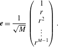 $$\begin{eqnarray}\boldsymbol{e}=\frac{1}{\sqrt{M}}\left(\begin{array}{@{}c@{}}1\\ r\\ r^{2}\\ \vdots \\ r^{M-1}\end{array}\right).\end{eqnarray}$$
The coefficient
 $1/\sqrt{M}$
is added to normalize the obtained eigenvectors.
Possible eigenvalues deduced from (B 6) are not unique, more precisely, the relation (B 6) is verified for
 $s$
different values of
 $\unicode[STIX]{x1D706}$
,
 $\{\unicode[STIX]{x1D706}_{0},\unicode[STIX]{x1D706}_{1},\ldots ,\unicode[STIX]{x1D706}_{M-1}\}$
, each one corresponding to a possible root of unity. Finally the set of possible eigenvalues corresponds to
 $$\begin{eqnarray}\unicode[STIX]{x1D706}_{s}=\mathop{\sum }_{p=0}^{M-1}c_{p}\exp (-2\text{i}\unicode[STIX]{x03C0}sp/M),\quad s=0,1,\ldots ,M-1.\end{eqnarray}$$
Equation (B 8) can be used to deduce eigenvalues associated with discrete expression of derivatives on a closed domain with periodic boundary conditions,
 $c_{k}\neq 0$
if
 $k\in [0,1,M-1]$
, the following simplified relation is obtained,
 $$\begin{eqnarray}\displaystyle \unicode[STIX]{x1D706}_{s} & = & \displaystyle c_{0}+c_{1}\exp (-2\text{i}\unicode[STIX]{x03C0}s/M)+c_{M-1}\exp (-2\text{i}\unicode[STIX]{x03C0}s(M-1)/M)\end{eqnarray}$$
 $$\begin{eqnarray}\displaystyle & = & \displaystyle c_{0}+c_{1}\exp (-2\text{i}\unicode[STIX]{x03C0}s/M)+c_{M-1}\exp (2\text{i}\unicode[STIX]{x03C0}s/M).\end{eqnarray}$$
Appendix C. Definition of functions used in resolution of diffusion equation
C.1 Common functions

C.2 MPI functions

C.3 OpenMP functions