2. Model construction

The spacecraft in this paper refers to a three-axis stabilisation spacecraft that is used for Earth observation and carries multiple sensors, which cannot work normally when exposed to strong light. The orientation of the solar energy cell array is the same as that of the axis $- {\boldsymbol{y}_\textrm{B}}$ in the spacecraft body frame $O{x_\textrm{B}}{y_\textrm{B}}{z_\textrm{B}}$, and the orientation of the camera is the same as that of the axis ${\boldsymbol{z}_\textrm{B}}$. In Earth observation missions, the observation effect is the most important goal, while the spacecraft's energy acquisition requirements are minor. This paper considers the orientation accuracy of the axis ${\boldsymbol{z}_\textrm{B}}$ to the Earth. The above attitude constraints can be divided into two types: mandatory pointing constraints and prohibited pointing constraints.

2.1. Reference attitude modelling

The definition of the reference attitude is the attitude considering the spacecraft's orientation accuracy to the Earth and Sun with different priorities.

When the spacecraft is in the reference attitude under ideal conditions, the axis ${\boldsymbol{z}_\textrm{B}}$ of the spacecraft body frame $O{\textrm{x}_B}{\textrm{y}_B}{\textrm{z}_B}$ points to the centre of the Earth, and the $- {\boldsymbol{y}_\textrm{B}}$ axis points to the centre of the Sun. However, the position vector of the Sun ${\boldsymbol{R}_{\textrm{sun}}}$ is typically not strictly vertical to the position vector of the Earth ${\boldsymbol{R}_{\textrm{earth}}}$. The reference attitude cannot be directly defined as the axis ${\boldsymbol{z}_\textrm{B}}$ coinciding with the line between the spacecraft and the centre of the Earth and the axis $- {\boldsymbol{y}_\textrm{B}}$ coinciding with the Sun position vector ${\boldsymbol{R}_{\textrm{sun}}}$.

Therefore, when the spacecraft is in the reference attitude, only the direction of the ${\boldsymbol{x}_\textrm{B}}$ axis is unique:

(1)\begin{equation}{\boldsymbol{x}_\textrm{B}} = \frac{{ - {\boldsymbol{R}_{\textrm{sun}}} \times {\boldsymbol{z}_O}}}{{|{{\boldsymbol{R}_{\textrm{sun}}}} |}}\end{equation}

where ${\boldsymbol{z}_O}$ is the axis $\boldsymbol{z}$ of the orbital coordinate system. The origin of the orbital coordinate system $O{x_O}{y_O}{z_O}$ is located at the mass centre of the spacecraft. The ${\boldsymbol{x}_\textrm{O}}$ axis points in the speed direction of the satellite. The ${\boldsymbol{z}_\textrm{O}}$ axis points to Earth's centre, is vertical and points in the direction of spacecraft flight. The ${\boldsymbol{y}_\textrm{O}}$ axis is defined by the ${\boldsymbol{x}_\textrm{O}}$ axis and the ${\boldsymbol{z}_\textrm{O}}$ axis according to the right-hand rule.

To calculate the ${\boldsymbol{y}_\textrm{B}}$ axis and the ${\boldsymbol{z}_\textrm{B}}$ axis of the spacecraft body frame, two auxiliary coordinate systems $O{x_{\textrm{earth}}}{y_{\textrm{earth}}}{z_{\textrm{earth}}}$ and $O{x_{\textrm{sun}}}{y_{\textrm{sun}}}{z_{\textrm{sun}}}$ are defined, shown in Formula (2), where ${\boldsymbol{x}_{\textrm{sun}}} = {\boldsymbol{x}_{\textrm{earth}}} = {\boldsymbol{x}_\textrm{B}}$. 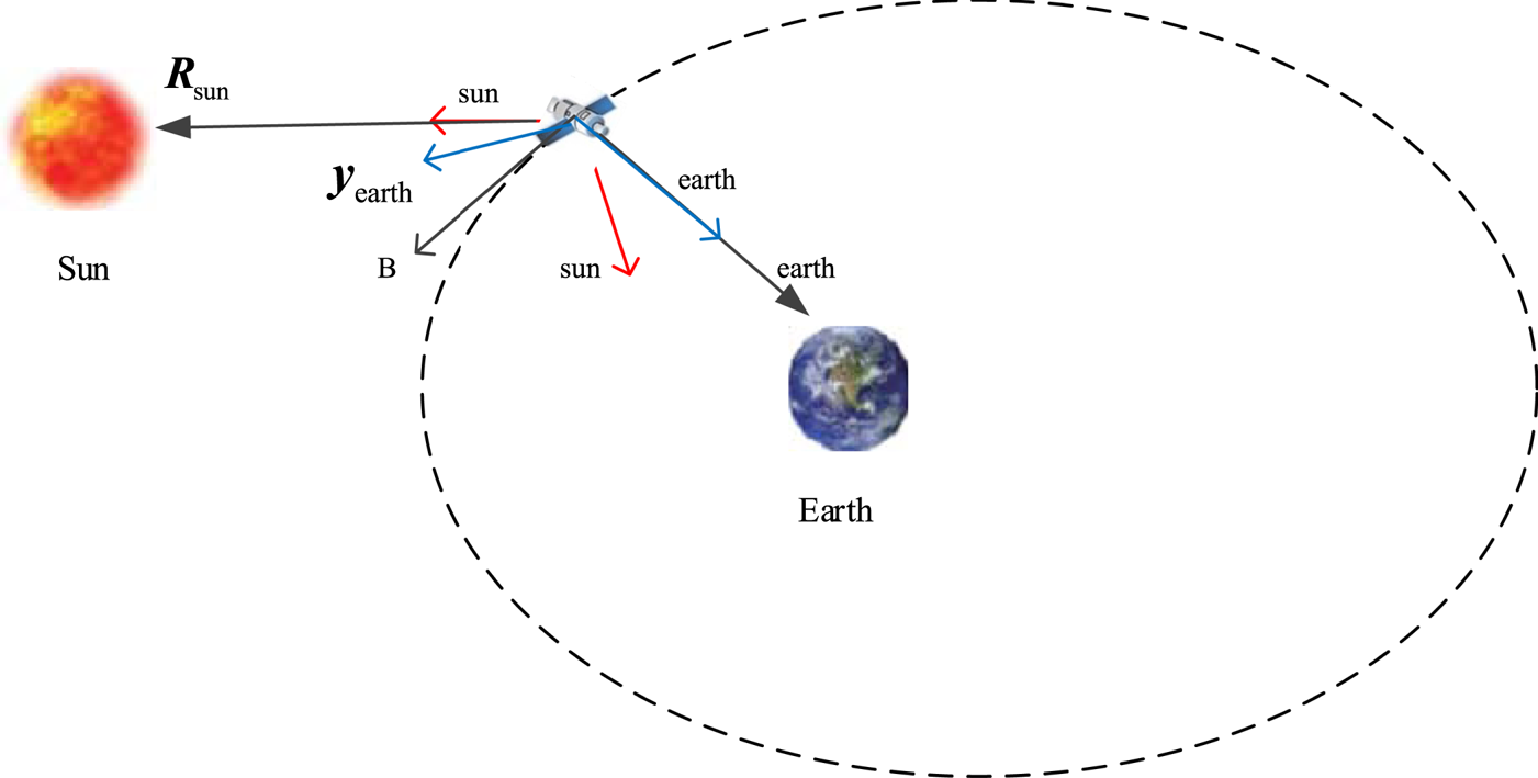The origin of auxiliary coordinate systems is the mass centre of the spacecraft. Figure 1 is a graphical representation of the relationship between auxiliary coordinate systems, the Earth and the Sun:

(2)\begin{equation}\left\{ \begin{array}{l} {\boldsymbol{z}_{\textrm{earth}}} = {\boldsymbol{z}_\textrm{O}},\\ {\boldsymbol{y}_{\textrm{earth}}} = {\boldsymbol{z}_{\textrm{earth}}} \times {\boldsymbol{x}_\textrm{B}}, \end{array} \right.\quad \left\{ \begin{array}{l} {\boldsymbol{y}_{\textrm{sun}}} ={-} \dfrac{{{\boldsymbol{R}_{\textrm{sun}}}}}{{|{{\boldsymbol{R}_{\textrm{sun}}}} |}}\\ {\boldsymbol{z}_{\textrm{sun}}} = {\boldsymbol{x}_\textrm{B}} \times {\boldsymbol{y}_{\textrm{sun}}} \end{array} \right.\end{equation}

Therefore, the spacecraft body frame coincides with $O{x_{\textrm{earth}}}{y_{\textrm{earth}}}{z_{\textrm{earth}}}$ when priority is given to the accuracy of the orientation to the Earth. The spacecraft body frame coincides with $O{x_{\textrm{sun}}}{y_{\textrm{sun}}}{z_{\textrm{sun}}}$ when the priority is given to the accuracy of the orientation to the Sun.

(3)\begin{equation}\left\{ \begin{array}{l} {\boldsymbol{y}_\textrm{B}} = \dfrac{{{\kappa_{\textrm{sun}}}{\boldsymbol{y}_{\textrm{sun}}} + {\kappa_{\textrm{earth}}}{\boldsymbol{y}_{\textrm{earth}}}}}{{|{{\kappa_{\textrm{sun}}}{\boldsymbol{y}_{\textrm{sun}}} + {\kappa_{\textrm{earth}}}{\boldsymbol{y}_{\textrm{earth}}}} |}}\\ {\boldsymbol{z}_\textrm{B}} = \dfrac{{{\kappa_{\textrm{sun}}}{\boldsymbol{z}_{\textrm{sun}}} + {\kappa_{\textrm{earth}}}{\boldsymbol{z}_{\textrm{earth}}}}}{{|{{\kappa_{\textrm{sun}}}{\boldsymbol{z}_{\textrm{sun}}} + {\kappa_{\textrm{earth}}}{\boldsymbol{z}_{\textrm{earth}}}} |}} \end{array} \right.\end{equation}

where ${\kappa _{\textrm{earth}}} \in [{0,1} ]$ and ${\kappa _{\textrm{sun}}} \in [{0,1} ]$ are weight coefficients.

Figure 1.

Graphical representation of auxiliary coordinate systems

According to Equations (1), (2) and (3), the reference attitude $({{\varphi_\textrm{d}},{\theta_\textrm{d}},{\psi_\textrm{d}}} )$ of the spacecraft can be described by:

(4)\begin{equation}\left\{ \begin{array}{l} {\varphi_\textrm{d}} = \arctan \dfrac{{{\boldsymbol{y}_\textrm{B}} \cdot {\boldsymbol{z}_\textrm{O}}}}{{{\boldsymbol{z}_\textrm{B}} \cdot {\boldsymbol{z}_\textrm{O}}}}\\ {\theta_\textrm{d}} = \arcsin ({ - {\boldsymbol{x}_\textrm{B}} \cdot {\boldsymbol{z}_\textrm{O}}} )\\ {\psi_\textrm{d}} = \arctan \dfrac{{{\boldsymbol{x}_\textrm{B}} \cdot {\boldsymbol{y}_\textrm{O}}}}{{{\boldsymbol{x}_\textrm{B}} \cdot {\boldsymbol{x}_\textrm{O}}}} \end{array} \right.\end{equation}

To describe the accuracy of the spacecraft's Earth orientation visually, the angle between axis ${\boldsymbol{z}_\textrm{B}}$ and axis ${\boldsymbol{z}_O}$ is introduced:

(5)\begin{equation}\cos \left\langle {{\boldsymbol{z}_\textrm{B}},{\boldsymbol{z}_\textrm{O}}} \right\rangle = {\boldsymbol{z}_\textrm{B}} \cdot {\boldsymbol{z}_\textrm{O}}\end{equation}

2.2. Attitude constraints modelling

The mandatory pointing constraints faced by the spacecraft include the energy acquisition constraints on the Sun and orientation constraints to the Earth. The prohibited pointing constraints refer to the sensor attitude constraints, including direct and reflected sunlight constraints.

The energy acquisition constraint states that the included angle between the solar light and the solar energy cell array is less than ${\theta _{q1}}$, and the included angle between the $- {\boldsymbol{y}_\textrm{B}}$-axis and the solar position vector ${\boldsymbol{R}_{\textrm{sun}}}$ in the spacecraft body frame is less than ${\theta _{q1}}$:

(6)\begin{equation}\cos \left\langle { - {\boldsymbol{y}_\textrm{B}},{\boldsymbol{R}_{\textrm{sun}}}} \right\rangle = \frac{{ - {\boldsymbol{y}_\textrm{B}} \cdot {\boldsymbol{R}_{\textrm{sun}}}}}{{|{{\boldsymbol{R}_{\textrm{sun}}}} |}} > \cos ({\theta _{q1}})\end{equation}

Orientation constraints on the Earth require that the included angle between axis ${\boldsymbol{z}_\textrm{B}}$ and Earth position vector ${\boldsymbol{R}_{\textrm{earth}}}$ in the spacecraft body frame be less than ${\theta _{q2}}$:

(7)\begin{equation}\cos \left\langle {{\boldsymbol{z}_\textrm{B}},{\boldsymbol{R}_{\textrm{earth}}}} \right\rangle = \frac{{{\boldsymbol{z}_\textrm{B}} \cdot {\boldsymbol{R}_{\textrm{earth}}}}}{{|{{\boldsymbol{R}_{\textrm{earth}}}} |}} > \cos ({\theta _{q2}})\end{equation}

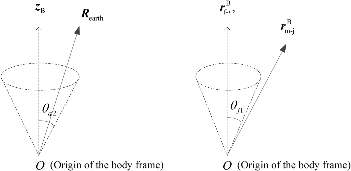
During attitude manoeuvring, it is necessary to avoid direct sunlight and reflected light areas within the conical fields of view of the sensors. Assuming that the position vector of the $i\textrm{th}$ central axis of the sensor's field of view in the spacecraft body frame is $\boldsymbol{r}_{\textrm{f}\hbox{-} i}^\textrm{B}$, the position vector of the $j\textrm{th}$ central axis of the reflected light area relative to the spacecraft is expressed as $\boldsymbol{r}_{\textrm{m}\hbox{-}j}^\textrm{B}$ in the spacecraft body frame. Figure 2 is a graphical representation of mandatory and prohibited pointing constraints. The position vector of the Sun is expressed in the spacecraft body frame as $\boldsymbol{r}_{\textrm{sun}}^\textrm{B}$. The prohibited pointing constraints require the included angle between $\boldsymbol{r}_{\textrm{f}\hbox{-}i}^\textrm{B}$ and $\boldsymbol{r}_{\textrm{m}\hbox{-}j}^\textrm{B}$ to be greater than ${\theta _{j\textrm{1}}}$ and the included angle between $\boldsymbol{r}_{\textrm{f}\hbox{-}i}^\textrm{B}$ and $\boldsymbol{r}_{\textrm{sun}}^\textrm{B}$ to be greater than ${\theta _{j\textrm{2}}}$:

(8)\begin{align}\cos \left\langle {\boldsymbol{r}_{\textrm{f}\hbox{-} i}^\textrm{B},\boldsymbol{r}_{\textrm{m}\hbox{-}j}^\textrm{B}} \right\rangle & = \frac{{\boldsymbol{r}_{\textrm{f}\hbox{-} i}^\textrm{B} \cdot \boldsymbol{r}_{\textrm{m}\hbox{-}j}^\textrm{B}}}{{|{\boldsymbol{r}_{\textrm{f}\hbox{-} i}^\textrm{B}} ||{\boldsymbol{r}_{\textrm{m}\hbox{-}j}^\textrm{B}} |}} < \cos ({\theta _{j1}})\end{align}

(9)\begin{align}\cos \left\langle {\boldsymbol{r}_{\textrm{f}\hbox{-} i}^\textrm{B},{\boldsymbol{R}_{\textrm{sun}}}} \right\rangle & = \frac{{\boldsymbol{r}_{\textrm{f}\hbox{-} i}^\textrm{B} \cdot {\boldsymbol{R}_{\textrm{sun}}}}}{{|{\boldsymbol{r}_{\textrm{f}\hbox{-} i}^\textrm{B}} ||{{\boldsymbol{R}_{\textrm{sun}}}} |}} < \cos ({\theta _{j\textrm{2}}})\end{align}

Figure 2.

Graphical representation of two types of constraint

3. Attitude manoeuvre planning for spacecraft based on reinforcement learning

Reinforcement learning can be divided into three categories: policy-based only, value-based only, policy-based and value-based. For a high-dimensional problem, it is difficult to isolate each state strictly and to calculate the value function of each state. The value-based only method has no explicit representation policy; thus, the change of the value function cannot reflect the change of the policy well. It is difficult to address the problem of random policy (Liu et al., Reference Liu, Gao and Luo2019). In contrast, the policy gradient algorithm always improves the policy by improving its direction and can effectively manage problems in the high and continuous action space (Tang et al., Reference Tang, Shao, Zhao and Zhu2017). For single-agent reinforcement learning, the optimal baseline and the low variance policy have been proven fruitful (Greensmith et al., Reference Greensmith, Bartlett and Baxter2004; Zhao et al., Reference Zhao, Gang, Ning, Yang and Masashi2015). Therefore, the policy gradient-based reinforcement learning method is used in this paper to perform attitude manoeuvre planning.

3.1. Attitude manoeuvre planning scheme design

Based on the reference attitude and attitude constraints model, this section describes the attitude manoeuvre planning scheme based on reinforcement learning. First, the reinforcement learning model of attitude planning is established, including the basic concepts of policy, reward function and policy value function. Second, the initial database for reinforcement learning is generated. In this paper, the reference attitude is used to establish the database, which can reduce the calculation of attitude manoeuvre planning and accelerate the convergence.

The total amount of data in the database is set to be N. Then, attitude manoeuvre planning is performed based on the improved policy gradient reinforcement learning algorithm. At the end of planning, $N + {k_{\textrm{tol}}}$ attitude manoeuvre trajectories will be obtained, where ${k_{\textrm{tol}}}$ is the total number of iterations.

The policy gradient reinforcement learning algorithm will update the Euler angle along the direction satisfying all constraints. However, it cannot guarantee that all $N + {k_{\textrm{tol}}}$ attitude manoeuvre trajectories meet the attitude constraint requirements. The accuracy is different for different trajectories. Therefore, the acquired attitude manoeuvre trajectories must be screened.

Before screening the results, it is necessary to define the screening index $\chi (k)$ for attitude planning results. The following is an optional screening index $\chi (k)$ for attitude planning results:

(10)\begin{align} \chi (k) & ={\upsilon _1}\min \left[ {\left\langle {{z_{\textrm{B},k}}(m),{z_{\textrm{O},k}}(m)} \right\rangle } \right] + {\upsilon _2}\min \left[ {\left\langle { - {y_{B,k}}(m),{R_{\textrm{sun},k}}(m)} \right\rangle } \right]\notag\\ & \quad + {\upsilon _3}[{\sigma ({{\varphi_k}(m)} )+ \sigma ({{\theta_k}(m)} )+ \sigma ({{\psi_k}(m)} )} ]\end{align}

where k represents the current iteration serial number; ${\upsilon _1}$,${\upsilon _2}$,${\upsilon _3}$ represent the weight coefficient; and $\sigma ({\ast} )$ represents the mean square deviation of ${\ast}$. The roll angle ${\varphi _k}(m)$, pitch angle ${\theta _k}(m)$ and yaw angle ${\psi _k}(m)$ are the three Euler angles of the spacecraft at moment m of the $k\textrm{th}$ iteration.

The screening index is not unique and can be designed according to real requirements. For the screening index proposed in this paper, the smaller the value is, the better the attitude planning result will be.

The final selected attitude planning result is the attitude manoeuvre planning result of group ${k_{\textrm{opt}}}$:

(11)\begin{equation}{k_{\textrm{opt}}} = \mathop {\arg }\limits_{{k^\ast }} \{{\chi ({k^\ast }) = \min [{\chi (k)} ],\quad k = 1,2, \ldots ,N + {k_{\textrm{tol}}}} \}\end{equation}

Flutter and other problems may exist in the final selected result, which will improve the difficulty of attitude control. Therefore, it is necessary to smooth the attitude planning results. The smoothing method is not unique. However, the attitude planning results after smoothing should still meet the requirements of attitude constraints. In this paper, the moving average filter is used to smooth the results.

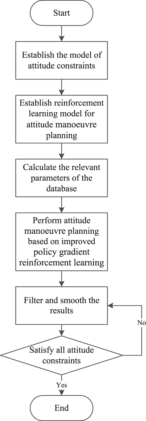
The flow of the attitude manoeuvre planning scheme based on reinforcement learning is shown in Figure 3.

Figure 3.

Flow chart of attitude manoeuvre planning

3.2. Attitude manoeuvre planning algorithm based on improved policy gradient reinforcement learning

3.2.1. Attitude manoeuvre planning model for reinforcement learning

The purpose of the policy gradient reinforcement learning method based on the finite difference policy gradient is to optimise policy ${x_k}(m)$ at the current moment m of iteration $k\textrm{th}$ based on policy value function $J[{{x_k}(m)} ]$:

(12)\begin{equation}J[{{x_{q,k}}(m)} ]= \sum\limits_{m = 1}^{{m_{\max }}} {\gamma (m){R_{q,k}}(m)}\end{equation}

where $\gamma (m)$ is the discount factor at this moment, and ${r_k}(m)$ is the reward function at time m.

The policy ${x_{k + 1}}(m)$ is updated as:

(13)\begin{equation}{x_{k + 1}}(m) = {x_k}(m) + \eta \nabla J[{{x_k}(m)} ]= {x_k}(m) + \eta G\end{equation}

where $\eta$ is the step size of reinforcement learning and G is the policy gradient.

The policy ${x_{q,k}}(m)({q = 1,2,3} )$ of the attitude manoeuvre is related to the Euler angles of the spacecraft:

(14)\begin{equation}\left\{ \begin{array}{l} {x_{1,k}}(m) = {\varphi_k}(m)\\ {x_{2,k}}(m) = {\theta_k}(m)\\ {x_{3,k}}(m) = {\psi_k}(m) \end{array} \right.\end{equation}

where ${x_{1,k}}(m)$, ${x_{2,k}}(m)$ and ${x_{3,k}}(m)$ represent the roll angle ${\varphi _k}(m)$, pitch angle ${\theta _k}(m)$, and yaw angle ${\psi _k}(m)$, respectively, of the spacecraft at time m of iteration $k\textrm{th}$.

The reward function shown in Equation (15) is related to the accuracy of the orientation to the Earth and the Sun and the prohibited pointing constraints:

(15)\begin{equation}\left\{ \begin{array}{l} {R_{\textrm{d,}k}}(m) ={-} {\mu_{\textrm{earth}}}\dfrac{1}{{{{\cos }^2}\left\langle {{\boldsymbol{z}_{\textrm{B,}k}}(m),{\boldsymbol{z}_{\textrm{O,}k}}(m)} \right\rangle }} - {\mu_{\textrm{sun}}}\dfrac{1}{{{{\cos }^2}\left\langle { - {\boldsymbol{y}_{\textrm{B,}k}}(m),{\boldsymbol{R}_{\textrm{sun,}k}}(m)} \right\rangle }}\\ {R_{\textrm{m}\hbox{-}i\textrm{,}k}}(m) ={-} \displaystyle\sum_{i = 1}^{{N_o}} {{\mu_{\textrm{f}\hbox{-} j-i}}{{\cos }^2}\left\langle {\boldsymbol{r}_{\textrm{f}\hbox{-}j\textrm{,}k}^\textrm{B}(m),\boldsymbol{r}_{\textrm{m}\hbox{-}j - i\textrm{,}k}^\textrm{B}(m)} \right\rangle } \\ {R_{\textrm{s,}k}}(m) ={-} \displaystyle\sum\limits_{j = \textrm{1}}^{{N_o}} {{\mu_{\textrm{sun}\hbox{-}i}}{{\cos }^2}\left\langle {\boldsymbol{r}_{\textrm{sun,}k}^\textrm{B}(m),\boldsymbol{r}_{\textrm{m}\hbox{-}j\hbox{-}i\textrm{,}k}^\textrm{B}(m)} \right\rangle } \end{array} \right.\end{equation}

where m is the moment, k is the current serial number of iterations, ${R_{\textrm{d,}k}}(m)$ is the reward function related to the orientation to the Earth and the Sun, and ${R_{\textrm{d,}k}}(m)$ in Equation (15) is the reward function of mandatory pointing constraints. There are two mandatory pointing constraints in this paper; thus, ${R_{\textrm{d,}k}}(m)$ consists of two fractions. If we must add new mandatory pointing constraints to the spacecraft, just add new fractions to ${R_{\textrm{d,}k}}(m)$.

${R_{\textrm{m}\hbox{-}i\hbox{-}j\textrm{,}k}}(m)$ and ${R_{\textrm{s,}k}}(m)$ represent reward functions of two different types of prohibited pointing constraints. ${N_o}$ represents the total number of sensors carried by spacecraft and ${N_J}$ represents the total number of reflected light areas. Therefore, ${N_o}$ and ${N_J}$ represent the number of two different types of prohibited pointing constraints. If we must add new prohibited pointing constraints to the spacecraft, just add new items to ${R_{\textrm{m}\hbox{-}i\hbox{-}j\textrm{,}k}}(m)$ or ${R_{\textrm{s,}k}}(m)$.

${R_{\textrm{m}\hbox{-}i\hbox{-}j\textrm{,}k}}(m)$ is the reward function related to the angle between the $i\textrm{th}$ central axis of the sensor's field of view and the $j\textrm{th}$ central axis of the reflected light area. ${\mu _{\textrm{f}\hbox{-}j\hbox{-}i}}$ is the weight coefficient of the reward function related to the included angle between the $i\textrm{th}$ central axis of the sensor's field of view and $j\textrm{th}$ the central axis of the reflected light area. ${R_{\textrm{s,}k}}(m)$ is the reward function related to the included angle between all central axes of the sensor's fields of view and the position vector of the Sun. ${\mu _{\textrm{f}\hbox{-}j\hbox{-}i}}$ is the weight coefficient of the reward function related to the included angle between the $i\textrm{th}$ central axis of the reflected light area and the position vector of the Sun. When the relevant included angle meets the attitude constraint requirements, the weight coefficient can be set to 0.

Because the attitude manoeuvre can be accomplished by circling the two coordinate axes of the spacecraft body frame, the total reward function of the policy is set as follows:

(16)\begin{equation}\left\{ \begin{array}{l} R[{{x_{1,n}}(m)} ]= R[{{\varphi_k}(m)} ]= {R_{\textrm{d},k}}(m)\\ R[{{x_{2,k}}(m)} ]= R[{{\theta_k}(m)} ]= {R_{\textrm{d},k}}(m) + \displaystyle\sum\limits_{j\textrm{ = }1}^{{N_J}} {{R_{\textrm{m}\hbox{-}i\hbox{-}j,k}}(m) + {R_{\textrm{s},k}}(m)} \\ R[{{x_{3,k}}(m)} ]= R[{{\psi_k}(m)} ]= {R_{\textrm{d},k}}(m) + \displaystyle\sum\limits_{j = 1}^{{N_J}} {{R_{\textrm{m}\hbox{-}i\hbox{-}j,k}}(m) + {R_{\textrm{s},k}}(m)} \end{array} \right.\end{equation}

The value function $J[{{x_{q,k}}(m)} ]$ of ${x_{q,k}}(m)({q = 1,2,3} )$ policy is:

(17)\begin{align}{R_{q,k}}(m) & = R[{{x_{q,k}}(m)} ]\end{align}

(18)\begin{align}J[{{x_{q,k}}(m)} ]& = \sum\limits_{m = 1}^{{m_{\max }}} {\gamma (m){R_{q,k}}(m)}\end{align}

3.2.2. Attitude manoeuvre planning algorithm based on improved policy gradient reinforcement learning

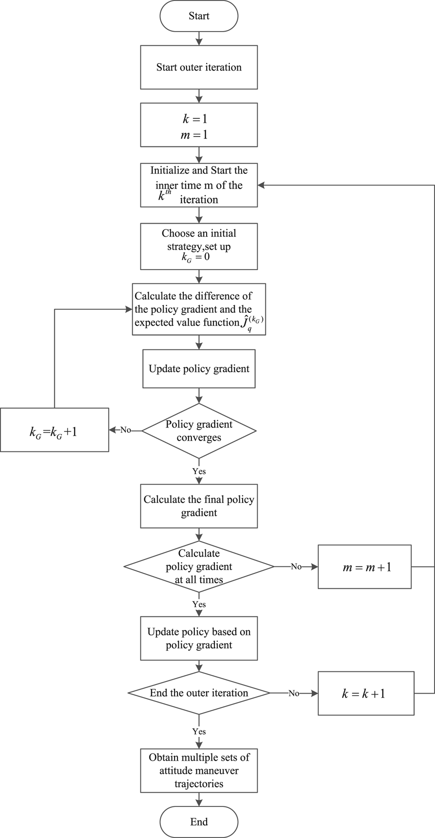
This section describes the process of the attitude manoeuvre planning algorithm based on improved policy gradient reinforcement learning. The process begins with the data in the database and then the outer iteration starts. First, initialise the serial number of iterations $k = 1$ and time $m = 1$.

To update the policy gradient, it is necessary to set the inner iteration. Let the current one be the ${k_G}$. Initialise ${k_G} = 0$. After the first generation, the initial policy at time m of the $k\textrm{th}$ iteration adopts the policy $x_{q,k}^{(0)}(m)$ at time m of the $k - 1\textrm{th}$iteration:

(19)\begin{equation}x_{q,k}^{(0)}(m) = {x_{q,k - 1}}(m)\end{equation}

Calculated reference expected value function $\hat{J}_{q,\textrm{ref}}^{({k_G})}$ of policy $x_{q,k}^{({k_G})}(m)$:

(20)\begin{equation}\hat{J}_{q,\textrm{ref}}^{({k_G})} = E[{\hat{J}[{x_{q,k}^{({k_G})}(m)} ]} ]= E\left[ {\sum\limits_{m = 1}^{{m_{\max }}} {\gamma (m){R_{q,k}}(m)} } \right]\end{equation}

where $E[{\cdot} ]$is the expect of $[{\cdot} ]$.${R_{q,n}}(m)$ is the reward of the policy of the $q\textrm{th}$ Euler angle at the moment.

$\varepsilon$ is a small value greater than zero. The policy $x_{q,k}^{(0)}(m)$ at time m of the $k\textrm{th}$ iteration satisfies $|{x_{q,k}^{(0)}(m) - x_{q,k}^{}(m)} |\le \varepsilon$.

In the inner iteration, the difference of the policy $\Delta x_{q,k}^{({k_G})}(m)$ must be calculated first, and then the expected value function $\hat{J}_q^{({k_G})}\,\, (q = 1,2,3)$ of $x_{q,k}^{({k_G})}(m) + \Delta x_{q,k}^{({k_G})}(m)$:

(21)\begin{align}\Delta x_{q,k}^{({k_G})}(m) & = \begin{cases} {x_{q,k - 2}}(m) - {x_{q,k - 1}}(m),\;{k_G} = 0\\ \eta {G_{q,k}}(m)\quad \quad \quad \quad \quad \,,\;{k_G} > 0 \end{cases} \end{align}

(22)\begin{align}\hat{J}_q^{({k_G})} & = E[{\hat{J}[{x_{q,k}^{({k_G})}(m) + \Delta x_{q,k}^{({k_G})}(m)} ]} ]\end{align}

(23)\begin{align}\Delta \hat{J}_{q,k}^{({k_G})}(m) & = \hat{J}_q^{({k_G})} - \hat{J}_{q,ref}^{({k_G})} - {R_{q,k - 1}}(m)/k - 1\end{align}

where $\Delta \hat{J}_{q,k}^{({k_G})}(m)$ is the expected value function difference with the return baseline, and ${R_{q,k - 1}}(m)$ is the return at time m of the $k - 1\textrm{th}$ iteration, where ${R_{q,k - 1}}(m)/k - 1$ is the return baseline. Generally, reinforcement learning algorithms based on policy gradients lack evaluation of policies. In some problems, the returns of the policy are always positive. Therefore, even a poor policy will be strengthened, resulting in a larger variance (Wang et al., Reference Wang, Fang and Li2015). To solve this problem, the return baseline is introduced to distinguish the quality of the strategy and reduce the variance of the policy gradient. To improve the calculation efficiency, this paper uses ${R_{q,k - 1}}(m)/k - 1$ to approximate the mean value the return baseline at time m of the $1\sim k - 1\textrm{th}$ iteration:

(24)\begin{equation}\left\{ \begin{array}{l} \Delta {\boldsymbol{x}_{q,k}}(m) = \left[ {\begin{array}{*{20}{c}} {\Delta x_{q,k}^{(0)}(m)}& {\Delta x_{q,k}^{(1)}(m)}& \cdots & {\Delta x_{q,k}^{({k_G})}(m)} \end{array}} \right]\\ \Delta {{\hat{\boldsymbol{J}}}_{q,k}}(m) = \left[ {\begin{array}{*{20}{c}} {\Delta \hat{J}_{q,k}^{(1)}(m)}& {\Delta \hat{J}_{q,k}^{(2)}(m)}& \cdots & {\Delta \hat{J}_{q,k}^{({k_G})}(m)} \end{array}} \right] \end{array} \right.\end{equation}

The policy gradient is updated to:

(25)\begin{equation}{G_{\textrm{temp},q,k}}(m) = \left\{ {\begin{array}{*{20}{l}} {0,}& {\Delta {\boldsymbol{x}_{q,k}}(m) = 0}\\ {{\mathop{\rm sgn}} \{{ - {{[{\Delta \boldsymbol{x}_{q,k}^\textrm{T}(m)\Delta {\boldsymbol{x}_{q,k}}(m)} ]}^{ - 1}}\Delta \boldsymbol{x}_{q,k}^\textrm{T}(m)\Delta {{\hat{\boldsymbol{J}}}_{q,k}}(m)} \},}& {\textrm{else}} \end{array}} \right.\end{equation}

We now introduce the error between policy ${x_{q,n}}(m)$ and reference attitude $x_{q,n}^\textrm{e}(m), (q = 1,2,3)$:

(26)\begin{equation} \begin{cases} x_{1,k}^\textrm{e}(m) = \varphi_k^\textrm{e}(m) = {\varphi_k}(m) - {\varphi_d}(m)\\ x_{2,k}^\textrm{e}(m) = \theta_k^\textrm{e}(m) = {\theta_k}(m) - {\theta_d}(m)\\ x_{3,k}^\textrm{e}(m) = \psi_k^\textrm{e}(m) = {\psi_k}(m) - {\psi_d}(m) \end{cases} \end{equation}

If ${G_{q,k}}(m)$ converges, reset${k_G} = 0$, and ${\mu _\textrm{e}} \ge 0$ is the weight coefficient. Then, calculate the final policy gradient ${G_{q,k}}(m)$:

(27)\begin{equation}{G_{q,k}}(m) = {G_{\textrm{temp},q,k}}(m) + {\mu _\textrm{e}}x_{q,k}^\textrm{e}(m)\end{equation}

If ${G_{q,k}}(m)$ does not converge, add ${k_G} + 1$ then repeat Equations (21)–(26) until the policy gradient converges.

In Equation (27), ${\mu _\textrm{e}}$ is a positive error weight coefficient less than 1, and $x_{q,n}^\textrm{e}(m)$ can guide the attitude of the spacecraft towards the reference attitude, which can mitigate any non-directionality in attitude updates. After obtaining the converged policy gradient at the current time, the time is updated until all times of the current outer iteration are completed.

Policy exploration is an important step in policy updating. If only the current obtained optimal policy gradient is used to guide updating, it can easily fall into a local optimum when the policy gradient is insufficient. A good policy exploration can consider other actions while learning the optimal actions and may find a better policy than the current one. Based on Equation (27), this paper proposes an adaptive exploration method for policy updating, as shown in Equation (28). ${c_1}$ is the fixed policy weight coefficient, ${c_{q1}}\ast \sin (k/{k_{\textrm{tol}}})\ast (\pi /2)$ is the dynamic policy weight coefficient, ${c_2}$ is the fixed exploration coefficient and ${c_{q2}}\ast \cos (k/{k_{\textrm{tol}}})\ast (\pi /2)$ is the dynamic exploration coefficient. In the early stage of the iteration, to keep the change in attitude stable, ${c_1}$ cannot be too large. However, ${c_2}$ can be marginally larger to enable the policy to gain stronger exploration ability and avoid falling into the local optimum prematurely. ${c_{q2}}\ast \cos (k/{k_{\textrm{tol}}})\ast (\pi /2)$ should increase gradually, and ${c_2}$ decreases gradually as the iteration progresses. The intention of the change is to balance the ability to follow the policy gradient and free exploration, which can speed up the process of convergence:

(28)\begin{align} {x_{q,k}}(m) & ={x_{q,k - 1}}(m) - ({c_1} + {c_{q1}}\ast \textrm{sin}\left(\dfrac{k}{{{k_{\textrm{tol}}}}}\ast \dfrac{\pi }{2}\right)\ast {G_{q,k}}(m)\notag\\ & \quad + ({c_2} + {c_{q2}}\ast \textrm{cos}\left(\dfrac{k}{{{k_{\textrm{tol}}}}}\ast \dfrac{\pi }{2}\right)\ast ({x_{q,k}}(m) - {x_{q,k - 1}}(m)) \end{align}

After updating the policy according to Equation (28), the outer iteration continues until the maximum number of iterations is reached. Finally, multiple groups of attitude manoeuvre planning trajectories were obtained to be screened.The flow chart of the algorithm proposed in this paper is shown in Figure 4.

Figure 4.

Flow chart of attitude manoeuvre planning based on improved policy gradient reinforcement learning

4. Simulation and analysis

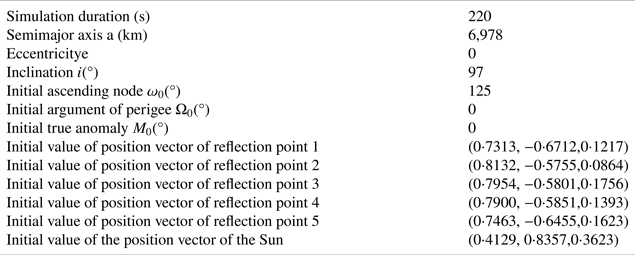
This paper analyses spacecraft operating in a Sun-synchronous orbit. The parameters of the orbit are shown in Table 1.

Table 1.

Parameters of Sun-synchronous orbit

Note: Time 1 January 2021 04:00:00⋅000 Universal Time Coordinated.

To gain a more intuitive understanding of the problem of attitude manoeuvre planning, this paper analyses a typical scene of spacecraft in orbit under complex and multi-constraint conditions first.

In this paper, sunlight is reflected by five reflection points on the surface of the Earth; thus, five reflected light areas will be formed. In the spacecraft body frame, the position vectors of the central axes of the sensor's field of view are:

(29)\begin{equation}\left\{ \begin{array}{l} \boldsymbol{r}_{\textrm{f}\hbox{-} 1}^B = {C_z}( - 50\;\deg ){C_y}(50\;\deg ){\left[ {\begin{array}{*{20}{c}} 1& 0& 0 \end{array}} \right]^T}\\ \boldsymbol{r}_{\textrm{f}\hbox{-} 2}^B = {C_z}( - 50\;\deg ){C_y}( - 50\deg ){\left[ {\begin{array}{*{20}{c}} 1& 0& 0 \end{array}} \right]^T}\\ \boldsymbol{r}_{\textrm{f}\hbox{-} 3}^B = {C_z}(50\;\deg ){C_y}(50\textrm{ }\deg ){\left[ {\begin{array}{*{20}{c}} 1& 0& 0 \end{array}} \right]^T}\\ \boldsymbol{r}_{\textrm{f}\hbox{-} 4}^B = {C_z}(50\;\deg ){C_y}( - 50\;\deg ){\left[ {\begin{array}{*{20}{c}} 1& 0& 0 \end{array}} \right]^T}\\ \boldsymbol{r}_{\textrm{f}\hbox{-} 5}^B = {\left[ {\begin{array}{*{20}{c}} 0& {\sin (60\;\deg )}& {\cos (60\;\deg )} \end{array}} \right]^T} \end{array} \right.\end{equation}

where ${\boldsymbol{C}_\textrm{z}}(\alpha )$ and ${\boldsymbol{C}_\textrm{y}}(\alpha )$ are the direction cosine matrices around the axis ${\boldsymbol{z}_\textrm{B}}$ and the axis ${\boldsymbol{y}_\textrm{B}}$, respectively.

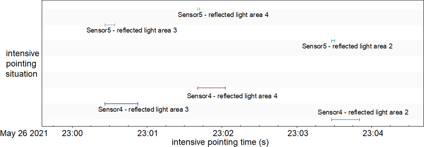
After preliminary analysis, the relative position relationship between the spacecraft and the reflected light areas changes periodically. We can thus draw the following conclusion: sometimes all fields of view for the sensors do not face any reflected light areas; sometimes sensors simultaneously face several reflected light areas in a short period of time, which means prohibited pointing constraints are violated. The selected most ‘dangerous’ situation is called the intensive pointing situation shown in Figure 5: in a short period of time, the fields of view of different sensors are successively directed to the reflected light areas. The next part of this paper focuses on the situation shown in Figure 5 (26 May 2021 23:00:26~23:03:51) to develop the attitude manoeuvre planning strategy.

Figure 5.

Intensive pointing situation

The simulation parameters are shown in Table 2. The position vectors of the central axes of reflected light areas and the Sun are both unit vectors in the Earth-centred inertial system.

Table 2.

Simulation parameters

This paper requires that the included angle between the $- {\boldsymbol{y}_\textrm{B}}$ axis and the position vector of the Sun be less than ${20^ \circ }$. In the spacecraft body frame, the included angles between the central axes of the sensor's fields of view and the central axes of the reflected light areas must be greater than ${30^ \circ }$. The included angles between all the central axes of the sensor's fields of view and the position vector of the Sun must be greater than ${40^\circ }$. 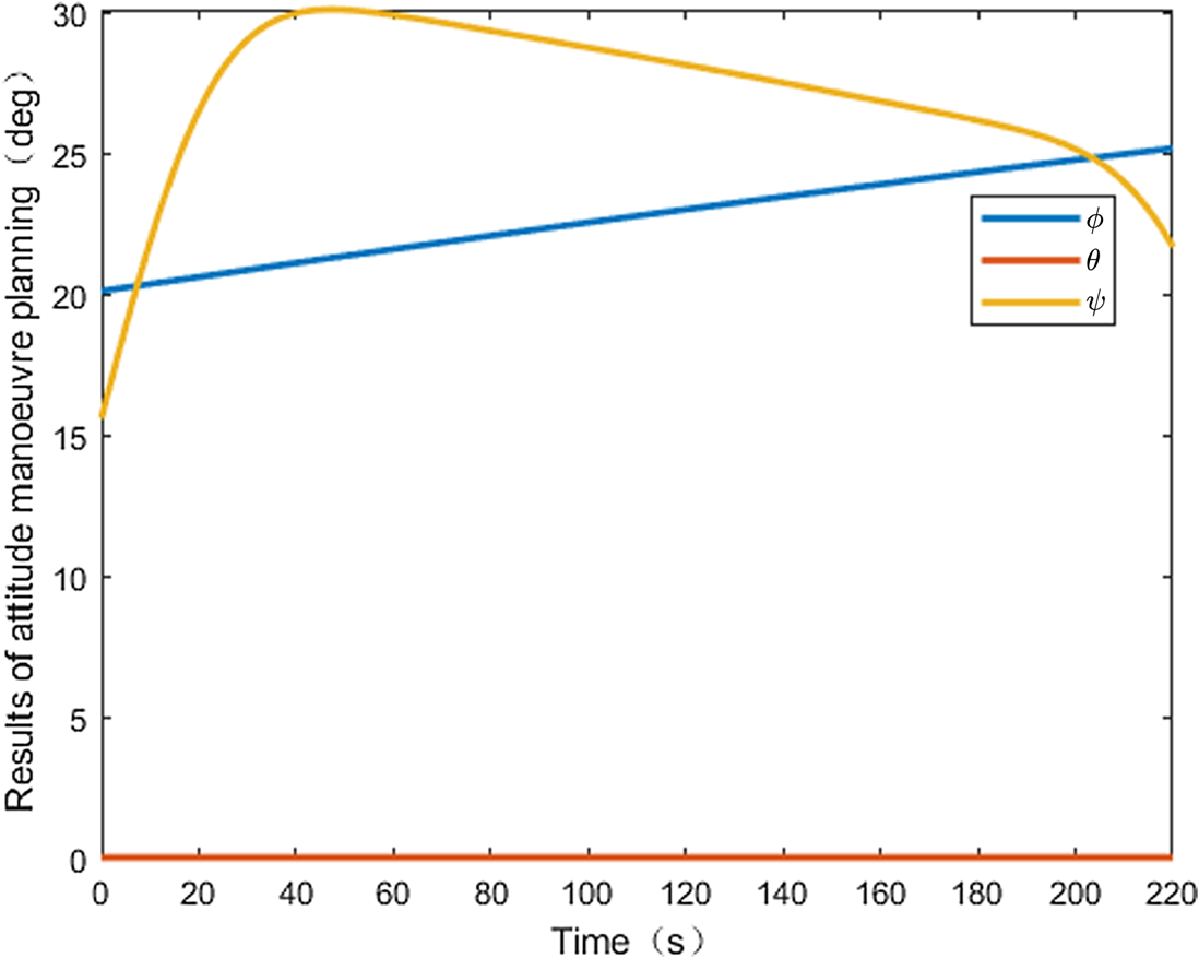After using the proposed algorithm to plan the spacecraft's attitude manoeuvre, the results of the attitude manoeuvre planning are finally obtained using Equation (10) as the screening index, as shown in Figure 6. The results of attitude manoeuvre planning in this paper leave a time margin of 10 seconds, which means that the attitude manoeuvre planning in all simulation results actually begins from the $10\textrm{th}$ second. Because the attitude adjustment of spacecraft can be accomplished by circling the two coordinate axes of the spacecraft body frames, Figure 6 shows that the change in pitch angle $\theta$ is nearly zero.

Figure 6.

Results of attitude manoeuvre planning

During the entire attitude manoeuvre planning time, the roll angle $\phi$ varies from $20{\cdot}37^{\circ }$ (in $10\textrm{th}$ second) to $25{\cdot}19^{\circ }$ (in $220\textrm{th}$ second). The yaw angle $\psi$ changes greatly. The minimum yaw angle is ${21{\cdot}86^\circ }$ (in $10\textrm{th}$ second), and the maximum yaw angle is ${30{\cdot}12^\circ }$ (in $46\textrm{th}$ second). Throughout the planning process, the change range is only ${8{\cdot}26^\circ }$.

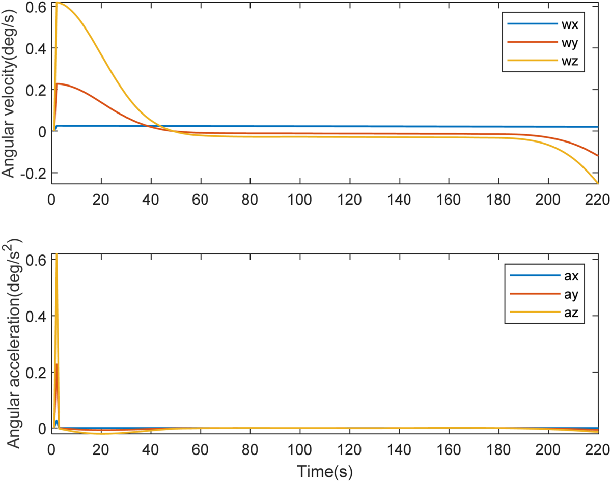
Figure 7 shows the components of angular velocity $\boldsymbol{w}$ and angular acceleration $\boldsymbol{a}$ of the attitude manoeuvre along the coordinate axes of the spacecraft body frame. The maximum value of the components of angular velocity is ${\boldsymbol{w}_z}$ in the $10\textrm{th}$ second, which is $0{\cdot}55^\circ{/}s$. The maximum absolute value of angular acceleration is ${\boldsymbol{a}_z}$ in the $20\textrm{th}$ second, which is $- 0{\cdot}021^\circ{/}{s ^{2}}$; this result indicates that in the planning time, the changing ranges of angular velocity and angular acceleration are very low. The changes in angular velocity and angular acceleration are small and slow, which is convenient for micro spacecraft.

Figure 7.

Angular velocity and angular acceleration

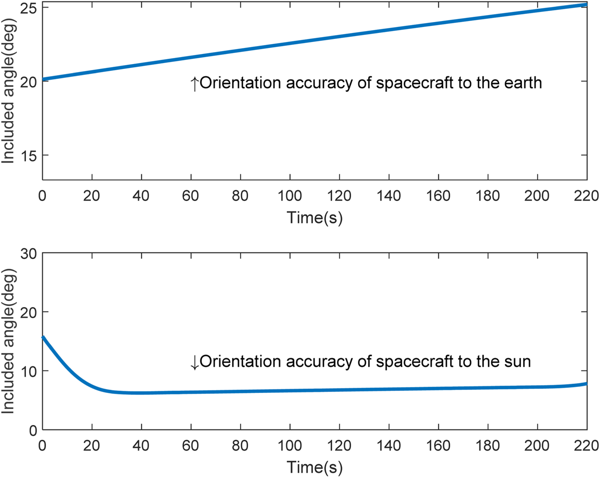
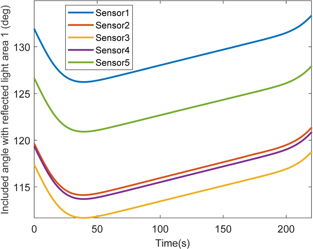
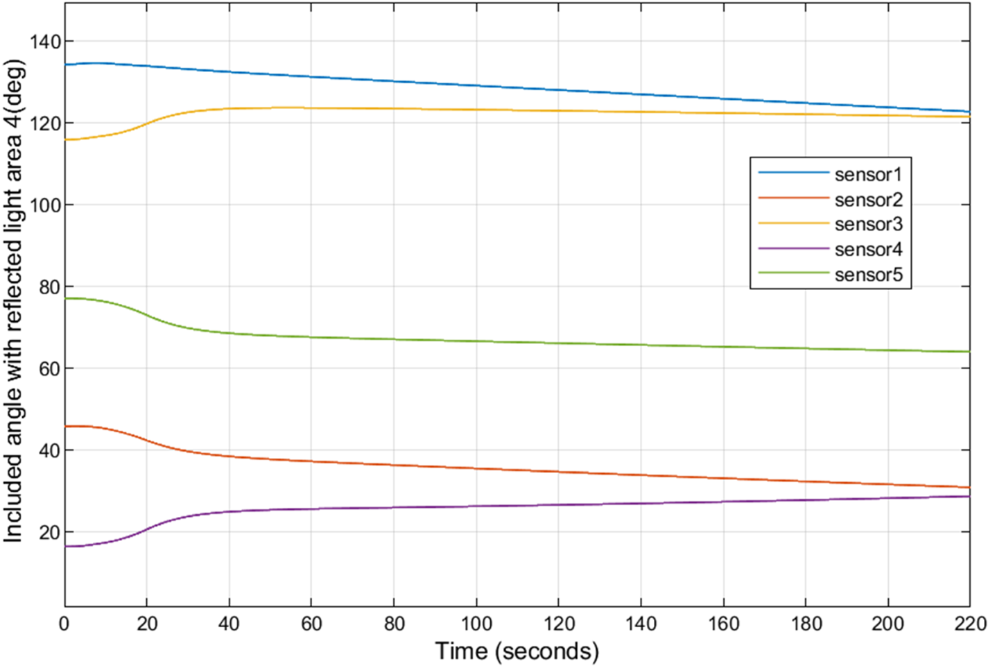
Although the changes in Euler angles are small, spacecraft still maintain a high orientation accuracy to the Earth and to the Sun, as shown in Figure 8. In most cases, the included angle between the $- {\boldsymbol{y}_\textrm{B}}$ axis and Sun is less than ${10^ \circ }$, which ensures the ability to gather solar energy. The included angles between the central axes of all reflected light areas and all central axes of the sensor's fields of view are shown in Figures 9–13. All fields of view for the sensors are far away from reflected light areas. The smallest included angle is ${41{\cdot}69^\circ }$ (the included angle between the centre axis of the sensor's field of view 2 and the reflected light area 2), which is still greater than ${30^\circ }$. In addition, as shown in Figure 14, the angle between the central axes of all sensor fields of view and the Sun position vector is larger than ${40^\circ }$, which effectively avoids sunlight.

Figure 8.

Orientation accuracy of spacecraft to the Earth and to the Sun

Figure 9.

Included angle between the central axes of the sensor field of view and the central axis of reflected light area 1

Figure 10.

Included angle between the central axes of the sensor field of view and the central axis of the reflected light area 2

Figure 11.

Included angle between the central axes of the sensor field of view and the central axis of the reflected light area 3

Figure 12.

Included angle between the central axes of the sensor field of view and the central axis of the reflected light area 4

Figure 13.

Included angle between the central axes of the sensor field of view and the central axis of the reflected light area 5

Figure 14.

Included angles between central axes of sensor attitude forbidden zones and the position vector of the Sun

Using the improved policy gradient reinforcement learning proposed in this paper, the spacecraft can effectively avoid dynamic direct and reflected sunlight while maintaining a high accuracy of pointing to the Earth and to the Sun. All sensors also avoid exposure to strong light with a large safety margin. The above results are not at the cost of a large attitude manoeuvre, and the process of changing the Euler angles in the planning results is smooth and slow, which conforms to the manoeuvrability of the micro spacecraft and can be executed smoothly by a control mechanism.

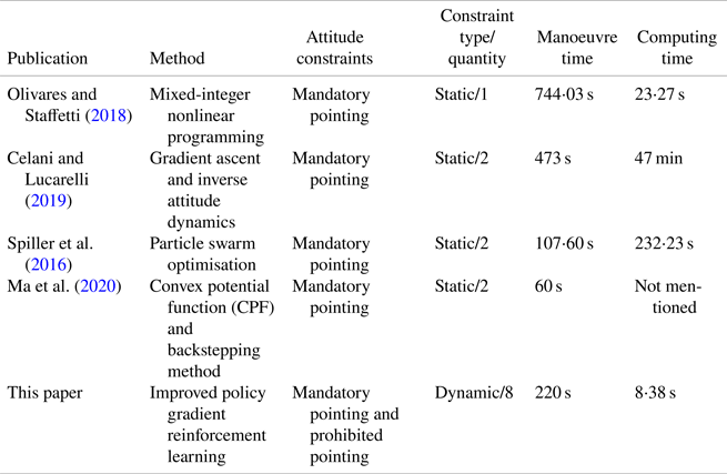
To demonstrate the originality and advantage of improved policy gradient reinforcement learning, the proposed method is compared with other relevant methods, which are shown in Table 3. Paper 5 in Table 3 shows the improved policy gradient reinforcement learning method proposed in this paper. The four methods in Table 3 represent different ideas to solve the problem of attitude manoeuvre planning.

Table 3.

Comparison with other methods

Table 3 shows that the first four methods only consider static constraints. The focus of the first three methods is the time-optimal reorientation manoeuvre problem of the spacecraft. In the above four methods, few static constraints exist on the virtual sphere, which makes the problem model too idealistic and far from the real-world situation. The start and end points of attitude are often known quantities when planning. These methods thus equate the known end point with mandatory pointing constraints, which cannot solve the problem of multiple mandatory pointing constraints concurrently. Compared with that method, the proposed method can successfully manage two dynamic mandatory pointing constraints concurrently in Sun-synchronous orbit, which is a difficult problem to solve.

The policy gradient reinforcement learning proposed in this paper is compared with the convex potential function (CPF) from Ma et al. (Reference Ma, Liu, Wang and Guo2020) to demonstrate its effectiveness. The relevant parameters are still set as shown in Table 2. To meet the need for orientation to the Sun, the desired attitude is defined: the included angle between the $- {\boldsymbol{y}_\textrm{B}}$ axis and the Sun is ${0^ \circ }$ if the spacecraft is defined in the desired attitude. The desired attitude expressed by Euler angles is shown in Figure 15. The results of attitude manoeuvre planning using the method of Ma et al. (Reference Ma, Liu, Wang and Guo2020) are shown in Figure 16. The orientation accuracies to the Sun and to the Earth are shown in Figure 17 and Figure 18, respectively.

Figure 15.

Desired attitude (CPF)

Figure 16.

Results of attitude manoeuvre planning (CPF)

Figure 17.

Orientation accuracy to the Sun (CPF)

Figure 18.

Orientation accuracy to the Earth (CPF)

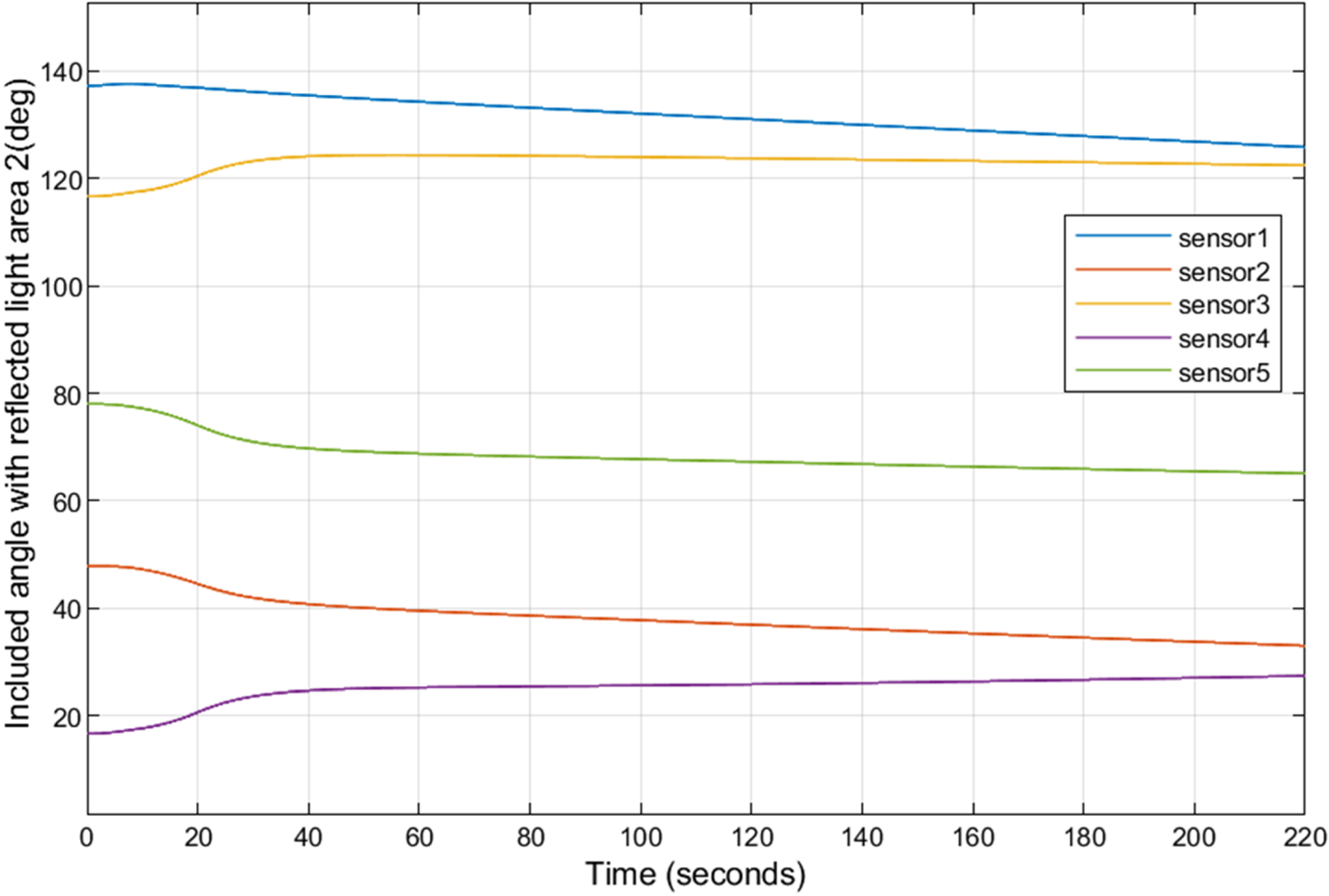
The planning results clearly do not track with the desired attitude. The included angle between the $- {\boldsymbol{y}_\textrm{B}}$ axis and Sun is much larger than ${20^\circ }$, which cannot meet the needs of power generation. The included angles between all central axes of reflected light areas and all central axes of the sensor's fields of view are shown in Figures 19–23. Note that the smallest included angle is smaller than ${30^\circ }$.

Figure 19.

Included angle with reflected light area 1 (CPF)

Figure 20.

Included angle with reflected light area 2(CPF)

Figure 21.

Included angle with reflected light area 3 (CPF)

Figure 22.

Included angle with reflected light area 4 (CPF)

Figure 23.

Included angle with reflected light area 5(CPF)

Figures 15–23 show that the CPF from Ma et al. (Reference Ma, Liu, Wang and Guo2020) does not seem to be suitable for solving the problems raised in this paper. The underlying reason for this result lies in Formula (16) of Ma et al. (Reference Ma, Liu, Wang and Guo2020), which is shown here as Equation (30):

(30)\begin{equation}V(\boldsymbol{\widetilde{e}}) = \sum\limits_{i = 1}^n {\frac{{{k_i}{{||\boldsymbol{e} ||}^2}}}{{{\mu_i} - {{\boldsymbol{\widetilde{e}}}^T}\overline {{\boldsymbol{A}_{\boldsymbol{i}}}} \boldsymbol{\widetilde{e}}}}}\end{equation}

where $\boldsymbol{\widetilde{e}}$ is the error quaternion when the desired attitude is given, and ${k_i} > 0$ are weight coefficients of different prohibited pointing areas in the potential function. Every prohibited pointing area has a threat zone, which is a set of attitudes, and weight coefficients are greater than zero (${k_i} > 0$) only if the attitude of the spacecraft is within the threat zone. However, once the attitude is adjusted outside the threat zone, the coefficient is equal to zero (${k_i} = 0$). When the attitude is outside all threat zones, all weight coefficients ${k_i}$ are equal to zero. When all ${k_i}$ are equal to zero, Equation (30) will equal zero because ${k_i}$ is part of the numerator. If the above situation occurs during the attitude manoeuvre planning process, the potential function will be invalid and the spacecraft will perform redundant invalid manoeuvres. In severe cases, the attitude control will be lost.

The first three methods in Table 3 require long computation times compared with the proposed improved policy gradient reinforcement learning method. In contrast, in the fourth method, the potential function combined with the backstepping method is efficient, and its focus is on using the control law to plan the attitude manoeuvre. The first step is to design an appropriate potential function and control law based on constraints. At this step, there is an inevitable problem in which the control parameters are difficult to design. On the premise of obtaining a suitable control law, the second step is to calculate the attitude manoeuvre trajectories based on dynamics and kinematics. However, the method proposed in this paper directly calculates the attitude manoeuvre trajectories, which indicates one step less than the control law method. From this perspective, this paper can be considered to provide a new idea for solving the problem of attitude manoeuvre planning.