





1. Introduction
In this work, we develop a machine learning (ML) surrogate model for predicting ion energy–angle distributions (IEADs) relevant to plasma–material interaction (PMI) in magnetic confinement fusion (MCF). IEADs determine how ions strike material surfaces, directly influencing sputtering, erosion and surface modification. Since the sputtering yield depends on both the ion impact energy
 $E_i$
(eV) and the impact angle
 $\theta$
relative to the surface normal, accurate knowledge of IEADs at the material boundary is essential for estimating erosion fluxes, surface evolution and component lifetimes.
In MCF conditions, ions leave the quasi-neutral plasma after being accelerated by the magnetic presheath (Chodura Reference Chodura1982) and the electrostatic Debye sheath (Tonks & Langmuir Reference Tonks and Langmuir1929); when radio-frequency (RF) heating systems are also present, an additional RF sheath forms (Butler & Kino Reference Butler and Kino1963; Myra Reference Myra2021). In conventional magnetised plasma sheaths, ions are accelerated by the sheath electric field, with energies and trajectories determined by plasma temperature, charge state, ion-to-electron mass ratio, and the strength and inclination angle of the magnetic field (Khaziev & Curreli Reference Khaziev and Curreli2015). While analytical models provide useful insights (Tonks & Langmuir Reference Tonks and Langmuir1929; Bohm Reference Bohm1949; Riemann Reference Riemann1991, Reference Riemann1994; Ahedo Reference Ahedo1997; Stangeby et al. Reference Stangeby2000; Lieberman & Lichtenberg Reference Lieberman and Lichtenberg2005; Chen Reference Chen2016; Moseev & Salewski Reference Moseev and Salewski2019), they typically oversimplify ion dynamics and nonlinear sheath behaviour. RF sheaths introduce additional complexity; the rectified RF-driven sheath potential can significantly exceed the thermal sheath drop and the sheath itself oscillates with the applied RF fields, dynamically altering ion trajectories. This produces more structured, anisotropic IEADs, which can enhance sputtering and modify the surface response. The time-dependent RF potential also introduces temporal variations in ion impact conditions, further complicating ion-material interactions.
High-fidelity particle-in-cell (PIC) simulations are the most reliable tool for modelling IEADs, as they track ion dynamics with self-consistent fields through thermal and RF sheaths. By resolving ion trajectories and RF-induced oscillations, PIC simulations provide kinetic-level accuracy of IEADs. However, their computational expense makes them impractical for device-scale applications where IEADs must be evaluated across entire first-wall and antenna structures. For example, the codes hPIC (Khaziev & Curreli Reference Khaziev and Curreli2018) and hPIC2 (Meredith et al. Reference Meredith, Rezazadeh, Huq, Drobny, Srinivasaragavan, Sahni and Curreli2023) have been used to resolve IEADs of thermal sheaths (Khaziev & Curreli Reference Khaziev and Curreli2015) and RF sheaths (Myra et al. Reference Myra, Elias, Curreli and Jenkins2020; Elias, Curreli & Myra Reference Elias, Curreli and Myra2021) with kinetic accuracy. Figure 1 shows two representative IEADs obtained from hPIC2 simulations for thermal (panel a) and RF sheath (panel b) conditions. Extending PIC simulations across an entire tokamak surface is prohibitively expensive, motivating the need for reduced-order surrogate models.
Examples of ion energy–angle distributions (IEADs) as obtained from hPIC simulations under (a) thermal sheath and (b) radio-frequency (RF) sheath conditions. Those two distributions are for illustrative purposes only, to show the nature of the two-dimensional distributions that the ML model will have to be able to reconstruct.

Machine learning (ML) based reduced order models are increasingly used in plasma fusion to accelerate simulations and improve predictive capabilities. They enable fast modelling of plasma behaviour, disruption forecasting and real-time control optimisation (Parsons Reference Parsons2017; Kates-Harbeck, Svyatkovskiy & Tang Reference Kates-Harbeck, Svyatkovskiy and Tang2019; Fu et al. Reference Fu, Eldon, Erickson, Kleijwegt, Lupin-Jimenez, Boyer, Eidietis, Barbour, Izacard and Kolemen2020). ML also helps uncover patterns in plasma dynamics and supports studies of material erosion, sputtering and impurity transport (Kino et al. Reference Kino, Ikuse, Dam and Hamaguchi2021; Lin et al. Reference Lin, Maurel-Oujia, Kadoch, Krah, Saura, Benkadda and Schneider2024). Additional applications include accelerating turbulence simulations, enhancing diagnostic interpretation, and aiding in the design of reactor components and materials (Piccione et al. Reference Piccione, Berkery, Sabbagh and Andreopoulos2020; Chang et al. Reference Chang, Ku, Hager, Churchill, Hughes, Köchl, Loarte, Parail and Pitts2021; Dong et al. Reference Dong, Wei, Bao, Brochard, Lin and Tang2021; Lao et al. Reference Lao2022).
Machine learning and surrogate models are revolutionising RF plasma heating research by drastically reducing computational complexity while maintaining high predictive accuracy. Multiple studies highlight this potential: Sánchez-Villar et al. (Reference Sánchez-Villar, Bai, Bertelli, Bethel, Hillairet, Perciano, Shiraiwa, Wallace and Wright2024, Reference Sanchez-Villar, Bai, Bertelli, Bethel, Hillairet, Perciano, Shiraiwa, Wallace and Wright2025) developed real-time ion cyclotron range of frequencies (ICRF) heating models using random forest and neural networks, achieving speedups of six to seven orders of magnitude and high regression scores. Wallace et al. (Reference Wallace, Bai, Sadre, Perciano, Bertelli, Shiraiwa, Bethel and Wright2022) similarly accelerated lower hybrid current drive simulations from minutes to milliseconds.
Reduced-order modelling approaches for the determination of IEADs have been previously explored. Seleson et al. (Reference Seleson, Mustafa, Curreli, Hauck, Stoyanov and Bernholdt2022) explored a least-squares fitting, sparse grid, coordinate transformation method for single-species thermal sheaths with up to 4 input parameters. While successful in reconstructing IEADs with 6–7 orders of magnitude speedup compared with hPIC simulations, these approaches are difficult to extend to larger parameter spaces or to RF sheaths. For example, with seven input parameters, over 19 000 simulations are required. Additionally, RF-induced IEADs often exhibit multi-peaked structures that are not well captured by coordinate transformation methods. Artificial Neural Networks (ANNs) offer a more scalable and flexible alternative. By training neural networks on large high-fidelity datasets of PIC simulations, surrogate models can reproduce IEADs with near PIC-level accuracy at a fraction of the computational cost.
Several neural network architectures are suitable for the current modelling task, each with distinct advantages and limitations. A fully connected multilayer perceptron (MLP) can directly map input vectors to the unrolled IEAD, but demands substantial memory for high-resolution outputs. Diffusion models (Sohl-Dickstein et al. Reference Sohl-Dickstein, Weiss, Maheswaranathan and Ganguli2015) offer high-quality distribution reconstruction, but require extensive training data, significant computational resources, and exhibit slower training and inference. Transformers with two-dimensional (2-D) positional encoding (Wu et al. Reference Wu, Peng, Chen, Fu and Chao2021; Vaswani et al. Reference Vaswani, Shazeer, Parmar, Uszkoreit, Jones, Gomez, Kaiser and Polosukhin2023) effectively capture global spatial dependencies, making them well suited for structured outputs, though they are computationally and memory intensive. FiLM-conditioned U-Nets (Meseguer-Brocal & Peeters Reference Meseguer-Brocal and Peeters2019) provide a flexible mechanism for incorporating conditioning information and are efficient for structured generation tasks, but may be less effective in modelling long-range dependencies.
In this paper, we present a machine learning surrogate model for reconstructing IEADs with PIC-level fidelity across a wide parameter space. The model combines multilayer perceptrons (MLPs) with convolutional neural networks (CNNs) in a hybrid deep deconvolutional neural network (DDeCNN) architecture, enabling fast and accurate emulation of IEADs under both thermal and RF sheath conditions. The motivations behind this architecture include its computational efficiency, support of multi-output design, spatial coupling and space invariance. The training datasets were generated using large-scale hPIC2 simulations covering a wide range of physical parameters (temperature, density, RF voltage, magnetic field angle and strength) and numerical parameters (time step, grid size, particles per cell). The multi-dimensional input parameter space was sampled using a Latin hypercube design (McKay, Conover & Whiteman Reference McKay, Conover and Whiteman1976) to ensure broad coverage. Testing and validation demonstrate that our ML surrogate model reproduces PIC-level IEADs at a fraction of the computational cost. The surrogate is constructed for both thermal and RF sheath conditions, including single- and multi-species plasmas, making it applicable to divertor, first-wall and RF-enhanced plasma–surface interaction scenarios. We systematically evaluate model accuracy using multiple error metrics (MAE, MSE, relative L2 norm) and demonstrate substantial computational speedups. The remainder of this paper is structured as follows. Section 2 details the problem set-up, datasets and neural network architecture. Section 3 presents results for thermal, RF and multi-species plasmas. Section 4 summarises conclusions and outlines future directions.
2. Methodology
This section describes the methodology used to construct and validate the machine learning surrogate model of ion energy–angle distributions (IEADs). We first summarise the physical problem (§ 2.1), then define the input parameter space (§ 2.2) and outline the data generation process using hPIC2 simulations (§ 2.3). Subsequent steps of data preprocessing, network design and error evaluation are discussed in §§ 2.4–2.7.
2.1. Physics problem description
The IEADs were obtained using the hPIC2 PIC code (Khaziev & Curreli Reference Khaziev and Curreli2018; Meredith et al. Reference Meredith, Rezazadeh, Huq, Drobny, Srinivasaragavan, Sahni and Curreli2023), which self-consistently resolves ion impact distribution functions in magnetised plasma sheaths. A sketch of the simulations domain is shown in figure 2. The simulation domain consists of a plasma slab bounded by two grounded plates (
 $V=0$
) in the presence of a magnetic field inclined at an angle
 $\psi _B$
relative to the surface normal, following the classic Chodura sheath configuration (Chodura Reference Chodura1982; DeWald, Bailey & Brooks Reference DeWald, Bailey and Brooks1987; Devaux & Manfredi Reference Devaux and Manfredi2006; Khaziev & Curreli Reference Khaziev and Curreli2015). A volumetric particle source maintains quasi-neutrality by replenishing particles lost to the walls. Ion motion is integrated in three spatial dimensions, while the electrostatic potential is solved along the direction perpendicular to the material wall. Thermal sheath cases were evolved to steady state, and the energy and impact angle of ions at the walls were recorded to construct the IEADs. For RF sheath simulations, boundary conditions were that we imposed antisymmetric sinusoidal plate voltages,
 $V_1 = V_{\mathrm{pp}} \sin ( \omega t )$
and
 $V_2 = V_{\mathrm{pp}} \sin ( \omega t - \pi )$
, where
 $\omega$
is the RF frequency and
 $V_{\mathrm{pp}}$
is the peak-to-peak applied voltage. This configuration produces rectified RF sheath potentials and reproduces the physics of RF rectification (Elias et al. Reference Elias, Curreli, Jenkins, Myra and Wright2019; Myra et al. Reference Myra, Elias, Curreli and Jenkins2020; Elias et al. Reference Elias, Curreli and Myra2021; Rezazadeh, Myra & Curreli Reference Rezazadeh, Myra and Curreli2023).
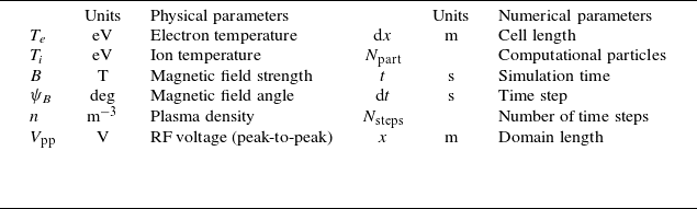
List of input parameters used in the ML model.

Sketch of the hPIC2 simulation domain under RF plasma sheath conditions. The figure illustrates a dual-plate structure driven by antisymmetric sinusoidal voltages,
 $V_1 = V_{\mathrm{pp}} \sin ( \omega t )$
and
 $V_2 = V_{\mathrm{pp}} \sin ( \omega t - \pi )$
, along with the volumetric plasma source and resulting sheath regions. For thermal sheath conditions, both boundaries are grounded
 $(V_1 = V_2 = 0)$
.

2.2. Definition of the input parameter space
The surrogate model must reproduce IEADs across a broad range of plasma and numerical conditions. The input vector therefore includes both physical parameters (governing sheath dynamics) and numerical parameters (governing PIC discretisation), summarised in table 1.
For thermal sheath cases, four physical parameters were varied: electron-to-ion temperature ratio (
 $T_e/T_i$
), plasma density
 $n$
, magnetic field magnitude
 $B$
and field angle
 $\psi _B$
. This choice follows from physical considerations and sensitivity studies in earlier work (Seleson et al. Reference Seleson, Mustafa, Curreli, Hauck, Stoyanov and Bernholdt2022; Mustafa Reference Mustafa2023).
For RF sheath cases, an additional parameter, the RF peak-to-peak voltage
 $V_{\mathrm{pp}}$
, was included. While using temperature ratio
 $T_e/T_i$
is adequate for describing normalised ion energy–angle distributions (IEADs) under steady thermal sheath conditions, it becomes insufficient in RF sheaths. The time-varying RF potential causes ions to experience phase-dependent acceleration, making the IEAD depend not only on
 $T_e/T_i$
, but also on the normalised RF amplitude
 $e V_{\mathrm{pp}}/T_e$
and the ratio of the RF period to the ion transit time
 $\omega _{\mathrm{RF}} \tau _i$
. Accordingly, in our model,
 $T_e$
and
 $T_i$
were treated as separate parameters, and an additional parameter
 $V_{\mathrm{pp}}$
(the RF peak-to-peak voltage) was introduced to capture these RF-induced effects.
Additionally, up to six numerical parameters (e.g. time step, cell length, particles per cell, domain length) were included as additional inputs. While not strictly ‘free’ physical parameters, including them ensures the ML surrogate captures subtle dependencies on discretisation and avoids misinterpreting numerical artefacts as physical trends. Constraints on these parameters are detailed in § 2.3 and Appendix A.
2.3. Data generation
Training and testing datasets were generated using high-resolution simulations run with the hPIC2 code (Meredith et al. Reference Meredith, Rezazadeh, Huq, Drobny, Srinivasaragavan, Sahni and Curreli2023). Additionally, we were also able to use a portion of training data from earlier studies (Seleson et al. Reference Seleson, Mustafa, Curreli, Hauck, Stoyanov and Bernholdt2022; Mustafa Reference Mustafa2023), which were obtained from the hPIC code (Khaziev & Curreli Reference Khaziev and Curreli2015). The two PIC codes share the same physics kernel and for the same inputs, provide identical output, the only difference being hardware (GPU) acceleration implemented in hPIC2, not present in hPIC. Output benchmarks between the two codes were run to guarantee consistency among datasets. The data generation process followed four steps.
-
(i) Sampling of input parameters. Ranges of physical parameters were selected to match conditions relevant to fusion edge plasmas (table 2) (Keilhacker et al. Reference Keilhacker, Lackner, Behringer, Murmann and Niedermeyer1982; Stangeby et al. Reference Stangeby2000; Porter et al. Reference Porter, Petrie, Rognlien and Rensink2010; Wesson & Campbell Reference Wesson and Campbell2011; Ciraolo et al. Reference Ciraolo2019; Pitts et al. Reference Pitts2019). Sampling employed a Latin hypercube sampling (LHS) design with corner points explicitly included, ensuring uniform coverage and good representation of extreme cases (McKay et al. Reference McKay, Conover and Whiteman1976, Reference McKay, Beckman and Conover1979), including Lloyd algorithm (Lloyd Reference Lloyd1982).
-
(ii) Evaluation of numerical parameters. For each sampled point, numerical resolution parameters (e.g. grid size, time step, particles per cell) were determined by enforcing resolution constraints to guarantee physical fidelity. Details are given in Appendix A.
-
(iii) Execution of hPIC2 simulations. Input files were automatically generated for each parameter set and run on the Campus Cluster at the University of Illinois Urbana Champaign. At the wall, ion impact energies and angles were recorded to build the IEADs.
-
(iv) Dataset organisation. Each database was divided into training, validation and testing subsets. Testing datasets were generated independently (not subsets of training data) to preserve statistical independence and provide unbiased performance evaluation.
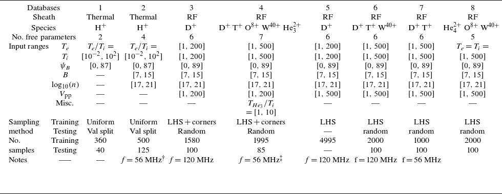
Summary of the databases generated using hPIC2 and used to train the ML model.

 $\dagger$
This database was also used for the data augmented (DA) model and served as the high-fidelity (HF) database for the multi-fidelity (MF) model, as discussed in § 3.2.1. After data augmentation, the total number of data points increases to 38 732.
 $\ddagger$
This database was used as the low-fidelity (LF) database for the MF model described in § 3.2.1. When the MF and DA models were combined, a total of 124 812 data points were augmented from this database.
Separate databases were created for thermal and RF sheaths, and for single- and multi-species plasmas (see table 2). The range of each free parameter is reported in table 2. Each dataset was first divided into two main subsets, training set and testing set. A portion of the training dataset was further split off as a validation set for hyperparameters tuning and model evaluation during training. The testing set was reserved exclusively for evaluating the model performance after training was complete. The model remains agnostic to the testing set, as it is not used at any point during the training or validation process. After selecting the hyperparameters, the validation dataset is merged back into the training set and the model is retrained using the combined data. To generate the training set, a total of
 $N_{\text{sample}}$
samples are drawn from the input parameter space. To ensure that these samples adequately cover the space, first we selected
 $2^{N_D}$
corner points of the input hypercube, where
 $N_D$
is the number of free parameters in the model. The remaining
 $N_{\text{sample}} - 2^{N_D}$
points are then generated using LHS (McKay et al. Reference McKay, Conover and Whiteman1976, Reference McKay, Beckman and Conover1979), with Lloyd algorithm (Lloyd Reference Lloyd1982), which iteratively relocates samples towards the centroids of their Voronoi cells to improve space-filling uniformity and minimise clustering. Furthermore,
 $N_{\text{test}}$
testing points are generated independently and randomly, separate from the training set. Although it is common to select testing data as a subset of the training dataset, doing so would reduce the number of available training points in what is already a sparsely sampled space. A routine was implemented to ensure that the testing data points do not overlap with, or closely resemble, the training or validation data points. Validation datasets were randomly sampled as a subset from the training dataset. In some cases, additional data augmentation was performed to increase temporal and spatial diversity (discussed in § 2.6).
2.4. Data normalisation
The input data span several orders of magnitude, which can negatively affect ML training by slowing convergence and biasing optimisation. Large variations in input scales can significantly slow down the convergence of gradient descent algorithms (Ioffe & Szegedy Reference Ioffe and Szegedy2015). Moreover, applying feature scaling is especially important when regularisation is used as part of the loss function, as unscaled features can lead to biased or unstable optimisation. To mitigate this, input features were normalised using min–max scaling (Patro & Sahu Reference Patro and Sahu2015),
 \begin{equation} x' = \frac {x - x_{\mathrm{min}}}{x_{\mathrm{max}} - x_{\mathrm{min}}}, \end{equation}
where
 $x$
is the raw value, and
 $x_{\mathrm{min}}$
,
 $x_{\mathrm{max}}$
are the limits of the sampled range. However, direct min–max scaling was not suitable for our output data (IEADs). This is because IEADs span many orders of magnitude: counts near the distribution boundaries may be very small, while the peak can be several orders larger. Using min–max would (i) obscure small but physically meaningful values at the tails and (ii) risk data leakage, since the maximum particle count is only known after the simulation. Instead, IEADs were preprocessed in two steps.
-
(i) Conversion to computational units. The accumulated physical particles were converted to computational counts using the physical-to-computational (
 $\mathrm{P2C}$
) ratio defined in hPIC2:(2.2)where
\begin{equation} {\mathrm{P2C}} = \frac {n x}{N_{\mathrm{PPC}} N_{\mathrm{cells}}}, \end{equation}
$n$
is particle density per unit volume,
$x$
is the domain size in [m],
$N_{\mathrm{PPC}}$
is the number of particles per cell and
$N_{\mathrm{cells}}$
is the number of cells.
-
(ii) Logarithmic scaling. The IEADs values were then transformed using a base-10 logarithm, which compresses the dynamic range while preserving the distribution shape.


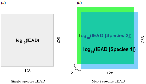
Data preparation of the IEADs is shown schematically in figure 16 reported in the Appendix. In the case of multi-species, IEADs are arranged as a four-dimensional (4-D) matrix [three-dimensional (3-D) matrix for each data point] as shown in figure 16( b ).
2.5. Machine learning models
The two neural network paradigms considered in this work were the following.
-
(i) MultiLayer perceptron (MLP/ANN). Classical fully connected feed-forward networks (Rumelhart, Hinton & Williams Reference Rumelhart, Hinton and Williams1986; Bishop Reference Bishop1995) with input, hidden and output layers. While straightforward, MLPs require large parameter counts to represent high-resolution distributions.
-
(ii) Convolutional neural networks (CNNs). Architectures that exploit spatial structure by applying learnable filters across input data (LeCun et al. Reference LeCun, Boser, Denker, Henderson, Howard, Hubbard and Jackel1989, Reference LeCun, Bottou, Bengio and Haffner2002; Alzubaidi et al. Reference Alzubaidi, Zhang, Humaidi, Al-Dujaili, Duan, Al-Shamma, Santamaría, Fadhel, Al-Amidie and Farhan2021). CNNs reduce parameter count, improve generalisation and are particularly well suited to 2-D outputs such as IEADs (treated as ‘images’).
MLP consists of interconnected nodes, known as neurons, organised in layers. These layers typically include an input layer, one or more hidden layers and an output layer. Information flows through the network from the input layer, where data are fed into the model, through the hidden layers, where computations are performed, to the output layer, which produces the model predictions or classifications. Each connection between neurons is associated with a weight that determines the strength of the connection. During the training process, these weights are adjusted iteratively to minimise the difference between predictions and outcomes.
Because IEADs are inherently 2-D distributions with strong spatial correlations, CNN-based methods were deemed essential. CNNs achieve regularisation by using fewer connections than MLPs and regularised weights. For instance, while a fully connected layer would demand an extensive number of weights to process a high-resolution image, CNNs efficiently reduce this requirement. Moreover, CNNs efficiently learn feature representations through filter optimisation, overcoming challenges like vanishing and exploding gradients, while simultaneously reducing computational complexity through hierarchical feature extraction.
2.6. Network architecture
For the reconstruction of IEADs, we developed a hybrid deep deconvolutional neural network (DDeCNN) that combines MLP and CNN elements (schematic in figure 3) structured as follows.
-
(i) MLP block. The input parameter vector passes through fully connected layers, progressively expanding the feature space and capturing nonlinear dependencies.
-
(ii) Reshape layer. The MLP output is reshaped into a low-dimensional matrix suitable for convolutional operations.
-
(iii) Deconvolutional block. A sequence of transposed 2-D convolutional layers (or informally, ‘deconv’ layers) progressively upsamples the matrix, doubling its height and width at each stage while reducing depth. This reconstructs the 2-D structure of the IEAD.
-
(iv) Final convolution. A 2-D convolutional layer reduces the output to one channel (single-species) or multiple channels (multi-species), matching the number of IEADs to be reconstructed.
Hybrid deep deconvolutional neural network (DDeCNN) architecture used to construct the machine learning surrogate model of ion energy–angle distributions (IEADs) from hPIC2 data. The input vector includes up to 13 parameters (up to seven physical and up to six numerical, listed in tables 1 and 2). These parameters are first processed through a multilayer perceptron (MLP), reshaped and passed into a sequence of transposed 2-D convolutional (‘deconv’) layers that progressively upsample the feature maps to reconstruct the 2-D IEADs. A final 2-D convolutional layer produces the output channels corresponding to the number of ion species. ReLU activations (Fukushima Reference Fukushima1969) are used throughout. The dashed blue box highlights the subset of layers that are frozen and unfrozen during multi-fidelity (MF) training, enabling knowledge transfer from low-fidelity to high-fidelity datasets.

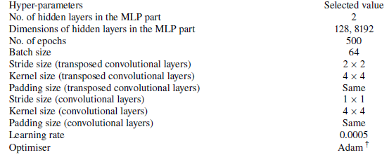
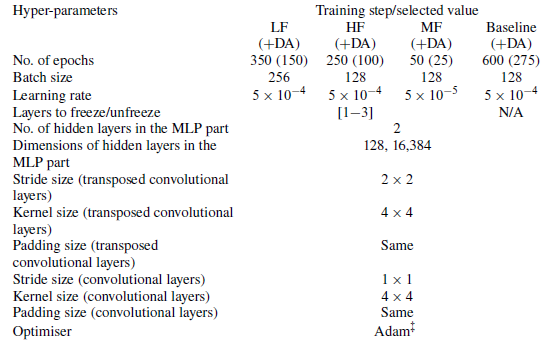
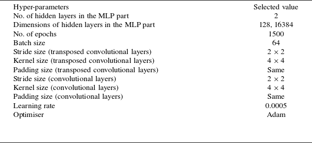
The rationale for this choice is driven by the 2-D nature of the IEADs. Pure MLPs are inefficient for large 2-D outputs, requiring excessive memory. Diffusion models (Sohl-Dickstein et al. Reference Sohl-Dickstein, Weiss, Maheswaranathan and Ganguli2015) and transformers (Wu et al. Reference Wu, Peng, Chen, Fu and Chao2021; Vaswani et al. Reference Vaswani, Shazeer, Parmar, Uszkoreit, Jones, Gomez, Kaiser and Polosukhin2023), while powerful, are computationally costly and require much larger training datasets. Deconvolutional CNNs exploit the structured nature of IEADs, enabling accurate and efficient reconstruction with fewer trainable parameters. All layers use the ReLU activation function (Fukushima Reference Fukushima1969), which mitigates vanishing gradients, introduces sparsity and preserves spatial continuity. Hyperparameters (learning rate, number of layers, filter sizes, etc.) were tuned via random search (Feurer & Hutter Reference Feurer and Hutter2019). Dataset-specific hyperparameter selections are reported in Appendix C.
Architecture enhancements. To extend the number of training data points in a given dataset without running more expensive PIC simulations, data augmentation was performed by extracting IEADs at different time steps and from different boundaries. This allowed expanding the dataset diversity at negligible cost and enabled the reconstruction of time-dependent IEADs necessary for RF sheath problems.
We also tested multi-fidelity (MF) learning. Since the number of high-fidelity (HF) data points available for training is limited, as shown in table 2, additional data can be generated at a reduced computational cost using the MF framework. To reduce reliance on expensive HF data, coarse-resolution hPIC2 simulations were used as low-fidelity (LF) data. Training proceeded in three stages: (i) pre-train on LF data; (ii) freeze early layers, retrain on HF data; and (iii) unfreeze all layers and fine-tune on HF data with reduced learning rate. This approach efficiently transferred trends from LF to HF, reducing overfitting and improving generalisation.
2.7. Error evaluation
No single metric can fully characterise surrogate accuracy. Therefore, three complementary error measures were used: the mean squared error (
 $\mathrm{MSE}$
), relative
 $\mathrm{L_2}$
norm error (
 $\mathrm{RL_2E}$
) and the mean absolute error per pixel (
 $\mathrm{MAE}$
). Each of these metrics captures different aspects of model performance.
 $\mathrm{MSE}$
emphasises larger errors due to its squared nature, making it sensitive to outliers and useful for identifying occasional large deviations.
 $\mathrm{RL_2E}$
provides a normalised measure of error relative to the magnitude of the true data, which is helpful for comparing performance across datasets or scales.
 $\mathrm{MAE}$
per pixel offers an intuitive average error per prediction unit, giving a straightforward sense of overall accuracy.
 \begin{align} \mathit{\mathrm{MSE}} &= \frac {1}{N \times M} \sum _{i=1}^N \sum _{j=1}^M \left ( y_{\textit{ij}} - \hat {y}_{\textit{ij}} \right )^2 , \end{align}
 \begin{align} \mathit{\mathrm{RL_2E}} &= \frac {\left [\sum _{i=1}^N \sum _{j=1}^M \left ( y_{\textit{ij}} - \hat {y}_{\textit{ij}} \right )^2\right ]^{{1}/{2}}}{\left [\sum _{i=1}^N \sum _{j=1}^M \left ( y_{\textit{ij}}\right )^2\right ]^{{1}/{2}}} , \end{align}
 \begin{align} \mathit{\mathrm{MAE}} &= \frac {1}{N \times M} \sum _{i=1}^N \sum _{j=1}^M \left | y_{\textit{ij}} - \hat {y}_{\textit{ij}} \right |, \end{align}
where
 $N$
and
 $M$
are the dimensions of the 2-D output,
 $y_{ij}$
is the actual data value of the
 $i{\mathrm{th}}$
angle and
 $j{\mathrm{th}}$
energy pixel indices, normalised between
 $[ 0, y_{ij}^{\mathrm{max}} ]$
(the number of particles accumulated on each pixel, as simulated by hPIC2), and
 $\hat {y}_{ij}$
is the ML-predicted value. For consistency, predicted IEADs were first denormalised (§ 2.4) and then rescaled by dividing by their maximum particle count, constraining all values between 0 and 1.
2.8. Computational resources
The generation of training and testing datasets required large-scale computational resources. All hPIC2 simulations were carried out on the University of Illinois Urbana–Champaign (UIUC) Campus Cluster, where up to 40 nodes were employed. Each node consisted of two Intel Xeon Processor E5-2670 v2 2.5 GHz with 10 cores each (20 cores per node) and 256 GB of RAM. On average, the generation of one database listed in table 2 required approximately five days using 40 nodes (
 ${\sim}100\,000$
CPU core-hours). Post-processing of the IEADs was performed using a local workstation equipped with dual Intel Xeon Processor E3 v3 and 96 GB of RAM.
Training and testing of the ML surrogate models were performed on GPU-powered systems. The primary training runs were conducted on the MIT Plasma Science and Fusion Center (PSFC) GPU cluster, where each node is equipped with four NVIDIA V100 GPUs, while additional experiments were performed on consumer-level equipment (NVIDIA GTX 1080 GPU) and industry-level high-end clusters (NVIDIA H100 Tensor Core GPUs). All workflows, including preparation of hPIC2 input files, post-processing of simulation outputs and ML model training, were implemented in Python. Neural network architectures were constructed and trained using the open-source libraries Keras (Chollet et al. Reference Chollet2015) and TensorFlow (Abadi et al. Reference Abadi2015), with supplementary data handling and preprocessing performed using scikit-learn (Pedregosa et al. Reference Pedregosa2011).
3. Results
3.1. Thermal plasma sheaths
The surrogate model was first evaluated under thermal sheath conditions for a single-species hydrogen plasma. This case was chosen as an initial benchmark because the resulting IEADs are relatively simple. The distributions can be described by a small set of parameters and they typically exhibit a single peak.
The training dataset consisted of 625 data points sampled uniformly across four free parameters: electron-to-ion temperature ratio (
 $T_e/T_i$
), magnetic field strength
 $B$
, plasma density
 $n_e$
and magnetic field inclination angle
 $\psi _B$
. Approximately 10 % validation split was applied, yielding 560 training samples and 65 testing samples. Hyperparameters for the DDeCNN model were selected through random search, with details provided in table 8 (Appendix C). Model performance was assessed using the three error metrics defined in § 2.7 (MAE, MSE and relative
 $L_2$
norm). For each metric, prediction errors were sorted and grouped into three categories: good (
 $E \lt \bar {E}$
), average (
 $\bar {E} \lt E \leqslant \bar {E} + 3 \sigma _E$
) and poor (
 $E \gt \bar {E} + 3 \sigma _E$
), where
 $\bar {E}$
is the mean error and
 $\sigma _E$
its standard deviation. Figure 4 illustrates this classification using MAE as the error measure, with representative cases from each category (labelled a, b, c) shown in figure 5.
Distribution of prediction errors for the thermal sheath database using the MAE metric. Errors are classified into three categories: good (
 $E \lt \bar {E}$
), average (
 $\bar {E} \lt E \leqslant \bar {E} + 3 \sigma _E$
) and poor (
 $E \gt \bar {E} + 3 \sigma _E$
). The majority of test cases fall in the good or average categories, with fewer than 3 % identified as poor. Representative cases from each category (labelled a, b, c) are highlighted and shown in detail in figure 5.

Comparison between hPIC2 IEADs (left column), ML surrogate predictions (middle column) and map of the difference between the IEADs of hPIC2 -ANN (right column) for three representative thermal sheath cases selected from figure 4. Case A (‘good’) illustrates excellent agreement, with the surrogate accurately reproducing both the peak and tails of the distribution. Case B (‘average’) demonstrates moderate deviations while maintaining the overall distribution shape. Case C (‘poor’) corresponds to a poor prediction. The associated MAE for examples A, B and C are
 $0.0067$
,
 $0.0191$
and
 $0.0376$
respectively.

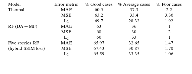
Overall, the ML surrogate reproduced the IEADs with high fidelity. Approximately 60 % of the test cases fell into the ‘good’ category, while fewer than 3 % were classified as ‘poor’ predictions (table 3). The small number of poor cases was primarily associated with simulations where the number of accumulated particles was too low, leading to noisy IEADs. In these situations, the ML model tended to smooth the noise because convolutional kernels inherently impose spatial coherence due to their shared-weight architecture, producing smoother but slightly biased reconstructions. Figure 5 compares three representative examples of ML predictions with the corresponding hPIC2 distributions. Case A (‘good’) demonstrates excellent agreement in both the peak and the tails of the IEAD. Case B (‘average’) shows moderate deviation but still reproduces the overall distribution shape. Case C (‘poor’) highlights the defects of a poor prediction; here, the original hPIC2 result was dominated by noise, which the ML model partially smoothed, but could not fully recover.
Additional evaluation using the MSE and relative
 $L_2$
norm confirmed the robustness of these results. According to the MSE metric, 63 % of predictions were classified as good, 33 % as average and 3 % as poor. Using the
 $L_2$
norm, the corresponding values were 70 %, 28 % and 2 %, respectively (table 3). These consistent statistics across multiple metrics confirm that the DDeCNN surrogate is able to reliably reproduce thermal sheath IEADs at a fraction of the computational cost of PIC. Table 3 shows a summary of error brackets for different metrics. More details on error statistics can be found in table 6 in Appendix B.
3.2. RF plasma sheaths
3.2.1. Single-species RF sheaths
The surrogate model was first tested for single-species deuterium plasmas in the presence of RF sheaths. Compared with the thermal sheath case, RF sheaths present a significantly more challenging prediction task. The oscillatory sheath potential introduces strong temporal modulation of ion acceleration, resulting in structured IEADs with multiple characteristic features. Instead of a single, nearly symmetric distribution, the RF IEADs exhibit broad energy spreads, RF-phase-dependent angular anisotropy and, in many cases, multi-peaked structures associated with ion mobility in the oscillating sheath. These features are particularly important for PMI studies, as they directly influence sputtering yields and surface modification. To address the added complexity of RF sheaths, we investigated more advanced surrogate modelling strategies, namely data augmentation (DA), multi-fidelity (MF) and a combined DA + MF approach.
Summary of the distribution of error brackets across all points in the thermal sheath dataset and RF sheath testing datasets based on various error metrics.

Construction of the RF database for DA and MF models. The RF database was constructed by sampling six physical parameters (
 $T_e$
,
 $T_i$
,
 $n$
,
 $B$
,
 $\psi _B$
and
 $V_{\mathrm{pp}}$
) and six numerical parameters (
 $\text{d}x$
,
 $x$
,
 $\text{d}t$
,
 $t$
,
 $N_{\mathrm{part}}$
,
 $N_{\mathrm{steps}}$
), as summarised in table 1. Although the numerical parameters are not strictly free inputs, their inclusion significantly improved prediction accuracy (see Appendix A). Additional training data were generated through augmentation of existing simulations, leading to the DA model. An MF learning strategy was also employed, using two datasets: an LF dataset (dataset 5, table 2) and an HF dataset (dataset 3, table 2). The LF dataset, generated with coarse discretisations, initially contained
 $4995$
cases, expanded via augmentation to
 $124\,812$
. The HF dataset, generated with fine discretisations, contained
 $1579$
cases, expanded to
 $38\,732$
. For testing, a separate HF-resolution dataset of
 $100$
cases was generated and augmented to
 $2475$
cases.
Training the DA and MF models. Training the MF model required careful hyperparameter optimisation due to its multi-stage design: (i) training on LF data; (ii) transfer learning on HF data; and (iii) hyperparameter fine-tuning. Additional hyperparameters specific to MF, such as the number and location of frozen/unfrozen layers, were optimised during this process. When DA was combined with MF, a new set of hyperparameters was required. The DA model suffered from overfitting due to redundancy in the augmented data, and thus required fewer training epochs. A random search strategy was used for hyperparameter tuning of both DA and MF + DA models. The final selected hyperparameters are summarised in table 9. After tuning, each model was retrained, and figure 6 shows how the MF model systematically outperformed the baseline by reducing the loss (MAE) across all training stages.
Evolution of the training loss function (MAE) during multi-fidelity (MF) training, compared with the baseline model. The three MF stages are shown: (i) initial training on the low-fidelity (LF) dataset; (ii) transfer learning on the high-fidelity (HF) dataset with partial layer freezing; and (iii) fine-tuning on HF data with all layers unfrozen. Each step yields systematic improvement over the baseline, demonstrating the effectiveness of the MF strategy.

Comparison across models. Figure 7 presents a systematic comparison of model accuracy using box-and-whisker plots of MAE. From left to right, the figure compares: the baseline model (no DA/MF), the DA model, the MF model and the combined MF + DA model, with ‘last step’ variantsFootnote
1
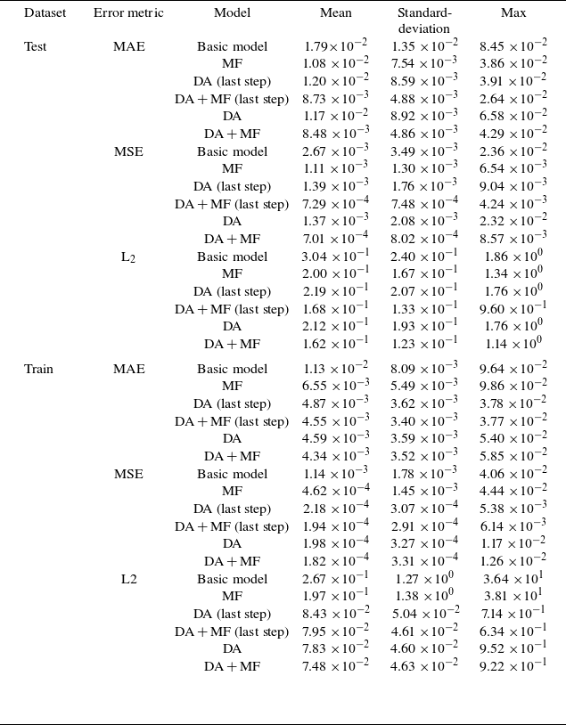
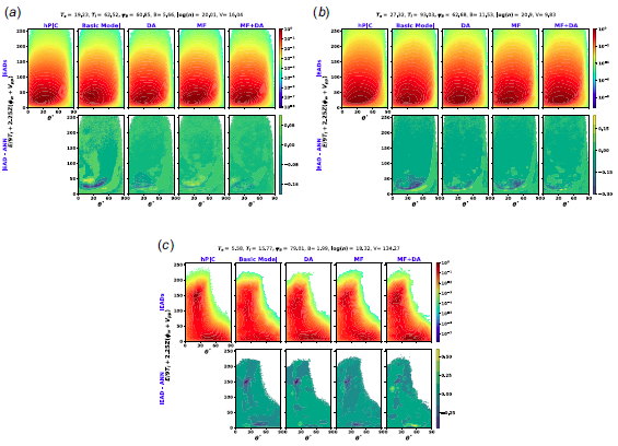
also shown for DA and MF + DA. While the baseline model performed reasonably well, both DA and MF reduced the mean and median MAE by approximately 50 % compared with the baseline model, with MF achieving slightly better results. Combining DA and MF further reduced the error by another 50 % relative to the already improved result. Variance was moderately reduced in the DA model and strongly reduced in MF and MF + DA. Interestingly, MF + DA did not substantially outperform MF alone in terms of mean and variance, but produced a more stable error distribution. Figure 9 shows a representative example where the surrogate accurately reproduced double-peak features caused by RF rectification. In most cases, the MF approach provided sufficient accuracy for practical applications, though both DA and MF introduced additional computational overhead: LF data generation increases simulation cost for MF, while DA greatly enlarges the training dataset, requiring efficient data handling. Notably, DA can emulate IEADs across multiple time steps, making it particularly valuable when transient behaviour is of interest. Trends observed in the MAE were consistent with those for MSE and
 $L_2$
error, as shown in figure 8. More details on error statistics can be found in table 7 in Appendix B.
Box-and-whisker comparison of the mean absolute error (MAE) for IEAD predictions for single-species RF sheaths across different surrogate models: baseline, data-augmented (DA), multi-fidelity (MF) and the combined DA + MF approach. Models trained on augmented datasets were also evaluated on the original data points (‘last step’ cases). In each plot, the central line marks the median, the red dot indicates the mean, the blue box spans the interquartile range (50 % of the data), whiskers extend to the minimum and maximum values, and black circles denote outliers. Both DA and MF substantially reduce error relative to the baseline, with MF + DA providing the most stable error distribution.

Distribution of error metrics for the training (red) and testing (blue) datasets. Data points within three standard deviations of the mean are shown for both MAE and
 $L_2$
error (
 $E_{\mathrm{MAE}}(i) \leqslant 3\sigma _{\mathrm{MAE}}$
,
 $E_{L_2}(i) \leqslant 3\sigma _{L_2}$
), while cases exceeding
 $3\sigma$
in MSE are marked with an ‘X’. Representative cases were identified using a weighted average of all three error metrics: the best, average and worst predictions in the training set are labelled A, B and C, respectively, while those in the testing set are labelled D, E and F. Detailed comparisons for these cases are provided in figure 9.

Example of IEAD predictions for a single-species RF sheath. The first row compares the reference distribution from hPIC2 (left) with the surrogate predictions from the baseline, data-augmented (DA), multi-fidelity (MF) and combined DA + MF models. The second row shows the corresponding residual error distributions for each model. The MF and DA + MF approaches most accurately reproduce the reference IEAD, including key features such as RF-induced broadening and multi-peaked structure, while also yielding smaller residuals. (Additional examples in figure 17.)

Time dependence. Some applications, such as RF-phase-resolved sputtering, turbulence studies and other plasma transient processes, require time-resolved IEADs. To evaluate model performance across time, we analysed the temporal evolution of MAE in the test dataset (figure 10). Combining MF with DA consistently reduced overall prediction error compared with DA alone, though the relative trends in error were preserved. High-error cases proved intrinsically more difficult to emulate, independent of the model. Elevated errors at early time steps were attributed to: (1) low particle statistics, which increase noise in the reference PIC data; and (2) transient plasma states, which reduce the representativeness of training samples. In some cases, errors increased at later stages, coinciding with the appearance of secondary peaks in the IEADs due to sheath rectification, which added structural complexity.
The surrogate models for RF sheaths also demonstrated strong predictive capability for single-species RF sheaths. Data augmentation and multi-fidelity strategies each improved accuracy relative to the baseline, with MF providing the most consistent gains and DA offering advantages for time-dependent cases. The combined MF + DA approach yielded the most stable error distributions, though at the cost of additional data preparation and training complexity.
To address whether it is more beneficial to increase the number of HF simulations or to adopt an MF modelling approach, we considered both structure and computational cost of our datasets. The MF approach offers clear advantages in our context. Although HF simulations provide highly accurate results, they are computationally expensive; each HF run takes approximately three times longer than an LF simulation. By leveraging both LF and HF data, the MF model efficiently uses the broader coverage of the LF dataset while preserving the precision of the HF data. Importantly, both datasets are generated using the same code (hPIC2) and resolve the physics accurately, with LF simulations already meeting high-quality standards (
 ${\sim}2000$
particles per cell) and HF simulations further reducing PIC noise (
 ${\sim}10\,000$
particles per cell). The strong correlation between LF and HF data enables the MF model to learn effectively from both sources. Additionally, the MF framework supports transfer learning, allowing the model to generalise across a wider parametric space or adapt to related tasks with minimal additional cost. These factors make the MF approach a more scalable and resource-efficient strategy compared with simply increasing HF samples.
To further evaluate the performance of the surrogate models, the sputtering yields computed using IEADs generated by hPIC are compared with those reconstructed using the surrogate models, as shown in figure 11. The comparison includes both the training and testing datasets, and considers two variations of the surrogate model: the basic model and the multi-fidelity model. The sputtering yield at each point in the IEAD is calculated using the methods described by Yamamura & Shindo (Reference Yamamura and Shindo1984) and Yamamura & Tawara (Reference Yamamura and Tawara1996), demonstrating the robustness of the surrogate models in accurately predicting sputtering yields.
Heatmaps of the mean absolute error (MAE) on the testing dataset as a function of time step. Results for (a) the stand-alone data-augmented (DA) model and (b) the combined DA + MF model. Colour bars indicate the error range, with markers denoting the maximum and minimum values for each model. The DA + MF approach reduces overall errors compared with DA alone, while preserving the temporal trends in model performance.

Comparison of sputtering yields calculated from distributions obtained using the ML surrogate model (y-axis), against sputtering yields obtained from PIC distributions (x-axis), for (a) training dataset and (b) testing dataset of RF sheath. Agreement between the two predictions is along the black dashed line. In each panel, two variations of the surrogate models are reported, namely basic model (light blue), and multi-fidelity model MF (light orange). Outlier cases classified as ‘poor’ predictions (
 ${\lt} 1.85$
% for the basic model and
 ${\lt} 0.49$
% for the MF model) have been highlighted in dark blue and dark red.

3.2.2. Multi-species RF sheaths
A more demanding test of the surrogate model involved plasmas containing multiple ion species in the presence of RF sheaths. Multi-species effects are ubiquitous in fusion-relevant plasmas, arising from fuel composition (D–T), fusion products (
 $\mathrm{He_4}$
), minority heating (
 $\mathrm{He_3}$
), intrinsic impurities (W, B, etc.), wall recycling and impurity seeding. Under RF sheath conditions, these mixtures generate particularly complex IEADs: each ion species responds differently to the sheath potential depending on its charge-to-mass ratio, leading to species-dependent broadening, overlapping distributions and modified angular anisotropy.
For this problem, we adopted dataset 4 in table 2, corresponding to a case with helium-3 minority heating. The surrogate was trained to emulate IEADs for five species simultaneously:
 $[\mathrm{D, T, O, He_3, W}]$
. Because the minority
 $\mathrm{He_3}$
population can reach temperatures well above the bulk ions, the helium-3 temperature
 $T_{\mathrm{He_3}}$
was included as an additional input parameter, defined as a multiple of the bulk ion temperature in the range
 $T_{\mathrm{He_3}} = [1{-}10] T_i$
. Unlike the single-species case, the outputs consisted of multiple IEADs, one per species, stored in separate output channels. This required a multi-output formulation of the surrogate, with the final convolutional layer producing multiple channels in parallel. Such a design ensured that correlations among species (e.g. common broadening due to the same sheath potential) were captured.
Training of multi-species problems. Training used 1995 independently generated cases and 100 test cases. Hyperparameter optimisation was performed via random search, with modifications introduced to handle the higher dimensionality of the multi-species problem (see table 10). The architecture was expanded to accommodate the multi-output design and the choice of loss function was carefully examined, since accurate representation of all species simultaneously required more than standard point-wise error minimisation.
Box plot comparing the performance of different loss functions in emulating the IEADs of five species. Performance is evaluated using the mean absolute error (MAE), averaged over all species, showing both training and testing datasets. The loss functions compared, from right to left, are mean squared error (MSE), mean absolute error (MAE), Wasserstein loss, Huber loss, structural similarity index measure (SSIM) and a hybrid SSIM–MAE loss.

Loss function comparison. Several loss functions were evaluated (figure 12): mean absolute error (MAE), mean squared error (MSE), Wasserstein loss (Frogner et al. Reference Frogner, Zhang, Mobahi, Araya and Poggio2015), Huber loss, structural similarity index measure (SSIM) and a custom hybrid SSIM–MAE loss. The hybrid loss combined pixel-wise accuracy with structural fidelity:
 \begin{equation} \mathcal{L}_{\mathrm{Hybrid}} = \alpha \boldsymbol{\cdot }\mathcal{L}_{\mathrm{SSIM}} + (1-\alpha ) \boldsymbol{\cdot }\mathcal{L}_{\mathrm{MAE}}, \quad \alpha =0.5, \end{equation}
where
 $\mathcal{L}_{\mathrm{SSIM}} = C - \mathrm{SSIM}$
and
 $C$
is a normalisation constant (typically
 $C=1$
). Neither MAE nor SSIM alone was sufficient. When training with these metrics, the model prioritised certain species while neglecting others, resulting in incomplete or blank IEADs. By contrast, the hybrid SSIM–MAE consistently outperformed the alternatives, producing lower mean error while preserving distributional structure. Huber and MSE achieved more constrained error distributions (lower variance), but at the expense of structural fidelity. Wasserstein performed worst overall. Figure 13 illustrates a representative case, comparing hPIC2 reference distributions (top row) with surrogate predictions trained under different losses. Models using the hybrid SSIM–MAE loss qualitatively preserved the multi-species features more effectively. Quantitatively, both MAE and
 $L_2$
error metrics confirmed the superiority of the hybrid approach.
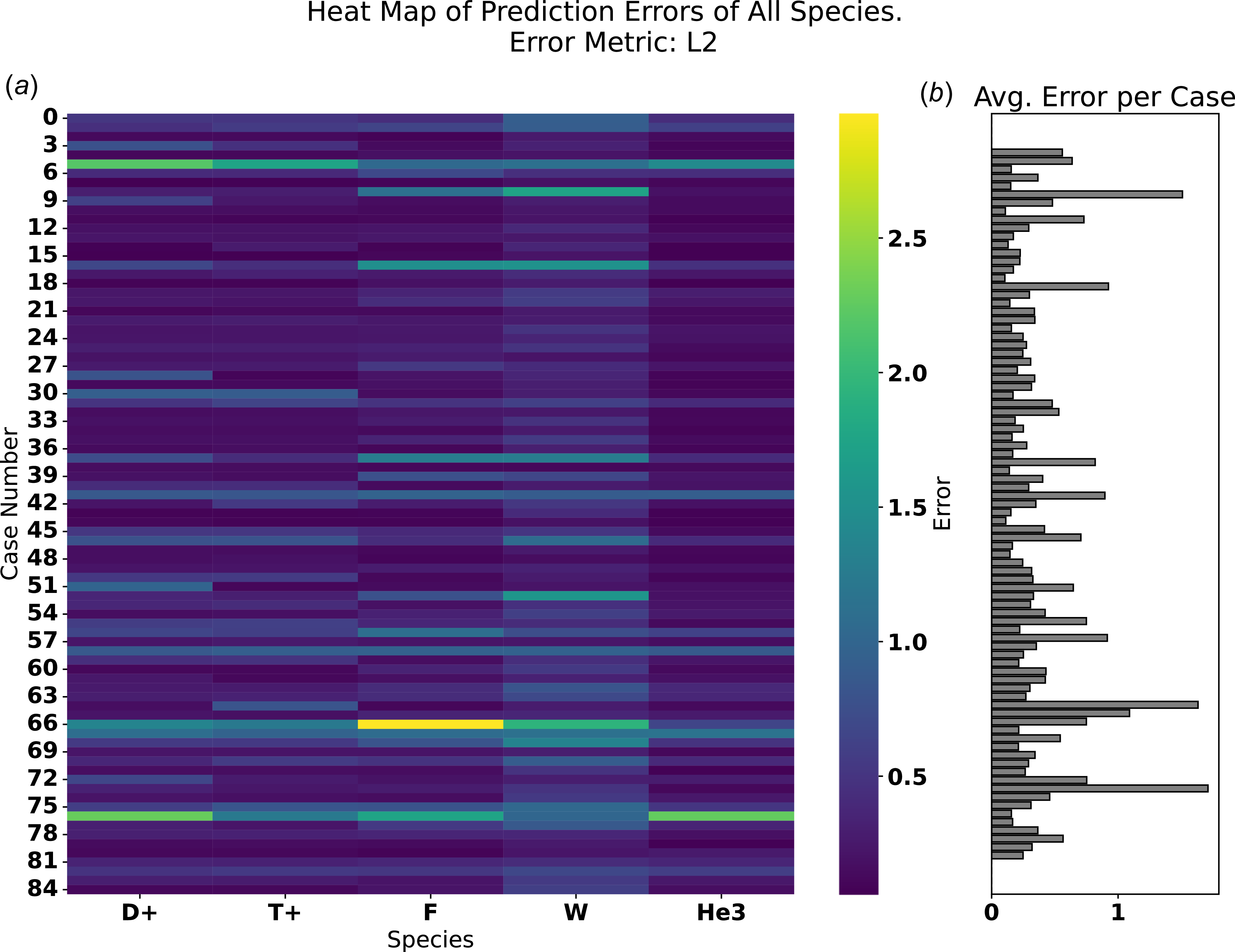
Species-dependent error behaviour. While figure 12 reports prediction error averaged over all species, figure 14 highlights error distributions for each species. Certain cases (e.g. #58, #67, #76) were consistently more challenging across all species, reflecting higher intrinsic complexity. Errors were generally larger for high-
 $Z$
species such as oxygen and tungsten, due to their stronger acceleration across the sheath potential. These ions undergo significant adiabatic cooling, producing narrower IEADs that are more sensitive to small deviations, which amplifies error metrics relative to broader distributions.
Overall, the surrogate successfully emulated IEADs for all five species simultaneously, provided that an appropriate architecture and loss function were used. The hybrid SSIM–MAE loss offered the best balance between structural fidelity and low error, while alternative losses performed less consistently. Species with narrow distributions (e.g. tungsten) were more sensitive to prediction deviations, but the surrogate captured their main features reliably.
Example of IEADs for a five-species plasma, comparing the reference hPIC2 results (top row) with surrogate predictions obtained using different loss functions (subsequent rows), illustrating the predictive performance of each loss function and the overall performance of the ML model for the multi-species RF sheath case. Superior accuracy in multi-species problems is obtained for the hybrid SSIM–MAE loss function.

(a) Heatmap of the
 $L_2$
error for each species across all cases in the testing dataset, highlighting species-specific error trends. (b) Bar plot of the mean absolute error (MAE) for each case, averaged over all species from the heatmap. Together, these plots show both case-by-case and species-resolved variations in prediction accuracy, emphasising that certain species and cases are intrinsically more challenging to emulate.

3.3. Time gain
A key advantage of the ML surrogate models lies in their dramatic reduction of computational cost relative to full PIC simulations. Generating a single IEAD with hPIC2 typically requires of the order of 12–24 h of wall-clock time on multiple CPU/GPU nodes, depending on plasma parameters and numerical resolution. In contrast, once trained, the DDeCNN surrogate can reproduce the same IEAD in less than one millisecond on a single GPU or less than a second on a standard CPU workstation. This corresponds to a speedup of approximately six to seven orders of magnitude.
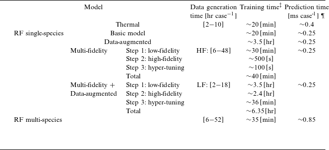
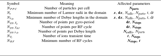
Table 4 shows a summary of the time required for: (i) dataset generation (an indication of total time spent on running PIC simulations); (ii) ML training; and (iii) ML prediction, for each of the databases used in this work. The time needed to generate each dataset can vary dramatically based on the number of data points in the database, numerical parameters (see table 5), number of input parameters and their ranges, and computer architecture used for data generation. Generally speaking, each of the eight databases of table 2 took
 ${\sim}5$
days to be generated using 40 nodes of the UIUC campus cluster (100 000 CPU core-hours). Time required for training also varies dramatically based on the size of data, the complexity of the architecture, number of epochs, etc.; a summary is reported in table 4. Training of the multi-species RF model is slightly more time consuming due to the increased complexity of the architecture used for that database. However, time required to train the DA models is significantly longer, due to the very large size of the database used for that model. Regardless of the specific surrogate architecture, the prediction time per data point remains nearly constant and depends only on the underlying GPU hardware, as illustrated in figure 15.
To emphasise the impact of this scalability, we considered a realistic application, computing IEADs across a detailed 3-D mesh made of 230 k surface nodes of an Ion Cyclotron Resonance Heating (ICRH) actuator, similar in geometry to the one in use within the WEST tokamak. This example was chosen for the geometrical complexity of the plasma-facing surfaces, due to the presence of RF limiters, Faraday rods, septa and corners within the RF actuator. Using hPIC2, such a calculation would require an estimated
 ${\sim}1000$
days of runtime on 40 nodes of the UIUC Campus Cluster. In contrast, the ML surrogate developed in this work reduces the same task to less than 2 minutes on a single GPU workstation. This result demonstrates the enormous efficiency gain achieved without compromising the fidelity of the original PIC model, enabling practical integration into device-scale PMI studies and design workflows. The implications of this gain are significant. Large-scale PMI studies often require IEADs to be evaluated at thousands of surface locations, under a wide variety of plasma conditions. Using direct PIC simulations for such studies is computationally prohibitive, since generating even 1000 IEADs would require several months of continuous use of a large computing cluster. By contrast, the surrogate can generate the same number of IEADs within minutes, enabling detailed PMI modelling and sensitivity studies that would otherwise be infeasible.
The efficiency gain is further amplified when considering parameter scans and optimisation studies. For example, in designing RF antenna systems for fusion reactors, the RF sheath response must be evaluated across a multi-dimensional parameter space involving density, temperature, magnetic field, RF voltage and geometry. Traditional PIC-based approaches can only afford to sample this space sparsely, whereas the surrogate allows dense sampling and RF-phase-resolved exploration. This makes it possible to perform probabilistic uncertainty quantification, surrogate-based optimisation and real-time coupling of sheath models with system-level codes.
Summary of the time required to train the ML models discussed in §§ 3.1 and 3.2, including the time required to train each step in the multi-fidelity models. Also showing emulation time for each IEAD following the training of the models.
 $^\dagger$

 $^\dagger$
Times listed in the table are based on NVIDIA RTX-1060Ti GPU for both training and prediction.
 $^\ddagger$
Based on NVIDIA RTX 1060 GPU.
¶For the entire dataset, based on NVIDIA RTX 1060.
User defined parameters that control the constrains. Parameters affected directly are highlighted in bold.

Inference time required to emulate multi-species IEADs with the ML surrogate, compared across CPU and several GPU architectures (RTX 1080 Ti, A10, A100 and H100). GPU acceleration reduces prediction time per case from seconds on CPU to milliseconds on modern GPUs, enabling six to seven orders of magnitude speedup relative to full PIC simulations. All time measurements are taken with the GPUs configured to run in double precision.

4. Conclusions
This work has demonstrated the development and application of machine learning surrogates for predicting ion energy–angle distributions (IEADs) in fusion-relevant plasma sheath conditions. Using data generated from the hPIC2 particle-in-cell code, we constructed and trained a deep deconvolutional neural network (DDeCNN) capable of accurately reproducing IEADs for both thermal and RF sheath regimes, including up to 13 input variables and up to five distinct plasma species.
The surrogate achieved high fidelity across a broad parameter space. For thermal sheaths, more than 97 % of test cases were classified as good or average predictions across multiple error metrics, with poor cases (
 $\lt$
3 %) occurring only in situations where hPIC2 results were affected by small statistical noise. For RF sheaths, which produce more structured, multi-peak IEADs, prediction accuracy remained robust, with 99 % of single-species and 98 % of multi-species test cases categorised as good or average. We show that the ML surrogate can reliably capture both the phase-space structure and magnitude of RF-driven IEADs.
In our work, we also explored several more advanced techniques, including data augmentation (DA) and multi-fidelity (MF) approaches. These methods enhanced the model’s ability to emulate complex distributions and allowed for significant reduction in training data requirements. Despite the limited number of training data points in some cases, the model demonstrated excellent performance, achieving high fidelity in predicting IEADs while maintaining inference times of the order of milliseconds. The DA approach, in particular, proved effective in capturing time-dependent behaviour, necessary for RF sheaths, making it especially promising for future studies involving transient plasma dynamics, such as transients, turbulence, etc.
Of particular relevance to practical applications, the ML surrogate delivers orders-of-magnitude improvement in computational efficiency. Once trained, the DDeCNN reproduces IEADs in milliseconds on a workstation, compared with hours or days required for PIC simulations on a supercomputing cluster. This corresponds to a speedup of six to seven orders of magnitude, effectively transforming IEAD generation from a computational bottleneck into a routine step that can be seamlessly integrated into larger whole-device frameworks. Such a gain makes it feasible to evaluate IEADs at thousands of wall locations, perform dense parameter scans, and couple sheath predictions directly with other PMI and erosion models. The ML surrogates developed in this study enable the incorporation of ion impact distributions, evaluated with PIC-level accuracy, into multiscale PMI modelling and reactor-relevant design studies.
Acknowledgments
Particle-in-cell simulations were run on the Illinois Campus Cluster, a computing resource operated by the Illinois Campus Cluster Program (ICCP) in conjunction with the National Center for Supercomputing Applications (NCSA) and supported by funds from the University of Illinois Urbana–Champaign (UIUC). Training, validation and testing of the machine learning models were performed on the Illinois Campus Cluster and using computing resources at the Plasma Science and Fusion Center (PSFC) at the Massachusetts Institute of Technology (MIT), Boston, Massachusetts. Proofreading of the final version of the manuscript was performed using GPT-5.0.
Editor Luís O. Silva thanks the referees for their advice in evaluating this article.
Funding
This material is based upon work supported by the U.S. Department of Energy, Office of Science, Office of Fusion Energy Sciences, under award number DE-SC0024369 (SciDAC Center for Advanced Simulation of RF-Plasma-Material Interactions). Additional support was provided under award DE-SC0025853 (FIRE Collaborative: APP-FPP Advanced Profile Prediction for Fusion Pilot Plant Design). Any opinions, findings and conclusions or recommendations expressed in this material are those of the author(s) and do not necessarily reflect the views of the U.S. Department of Energy.
Declaration of interests
The authors declare that they have no known competing financial interests or personal relationships that could have appeared to influence the work reported in this paper.
Appendix A. Quantitative constraints on numerical parameters
After generating the training and testing datasets through structured sampling of the free parameter space, each hPIC2 simulation configuration is evaluated using a set of logical conditions designed to enforce constraints on the numerical parameters. These constraints ensure that the simulations are sufficiently well resolved. The user-defined parameters that control the strictness of these constraints are listed in table 5. The specific numerical requirements are discussed as follows.
The size of the domain
 $x$
and element size
 $dx$
are computed based on the Debye length of the multi-species plasma
 $\lambda _D$
given by (A1) and the maximum value of Larmor radii
 $r^j$
of all ion species given by (A2), where
 $\epsilon _0$
is the permittivity of free space;
 $K_B$
is Boltzmann constant;
 $e$
is the elementary charge;
 $n_e$
is plasma density;
 $T_e$
is electron temperature;
 $B$
is the magnetic field strength; and
 $Z^j$
,
 $n^j$
and
 $T_i^j$
are respectively the charge, density and temperature of the
 $j\mathrm{th}$
ion species. Here,
 $v_\perp ^j$
is the speed perpendicular to the magnetic field, which is approximated as the most probable thermal speed of the
 $j\mathrm{th}$
ion species given by
 $v_\perp ^j = \sqrt {{2 T_i^j}/{m^j}}$
. Therefore,
 $dx$
is always selected as one Debye length
 $\lambda _D$
and the domain size
 $x$
is the largest of
 $500 \; \lambda _D$
or 3 times the largest value of
 $r_L$
.
 \begin{align} \lambda _D &= \left ( \frac {\epsilon _0 K_B/e^2}{n_e/T_e + \sum _j Z^j n^j T_i^j} \right )^{1/2}, \end{align}
 \begin{align} r_{\mathrm{max}} &= {\mathrm{max}}(r^j) = {\mathrm{max}} \left (\frac {m^j v_\perp ^j}{Z^j e B} \right )\! . \end{align}
Using (A1) and (A2), and the user defined parameters in table 5, the domain size
 $x$
is computed as follows:
 \begin{equation} x = \max \left [ N_{\lambda _D} \times \lambda _D , 3 \times \max \left ( r^j \right ) \right]\!, \end{equation}
and the element size is calculated using the value of points per Debye length
 $N_{\mathrm{pp}, \lambda _D}$
. In the case where
 $N_{\lambda _D} \times \lambda _D \leqslant 3 \times \max ( r^j)$
,
 $N_{\mathrm{\mathrm{pp}}, \lambda _D} = N_{\lambda _D}$
or
 \begin{equation} \mathrm{d}x = N_{\mathrm{pp}, \lambda _D} (x/\lambda _D). \end{equation}
Four constraints are enforced on the time step
 $\mathrm{d}t$
. The constraints are denoted as, thermal time step
 $\mathrm{d}t_{\mathrm{th}}$
, gyro time step
 $\mathrm{d}t_g$
, RF sheath ion transient time
 $\mathrm{d}t_{\mathrm{RF}}$
and RF period sampling frequency
 $\mathrm{d}t_T$
. The degree at which the constraints are enforced is controlled by the user-defined parameters as shown in table 5.
Following the determination of
 $\mathrm{d}x$
,
 $\mathrm{d}t_{\mathrm{th}}$
is computed as follows:
 \begin{equation} \mathrm{d}t_{\mathrm{th}} = \frac {\mathrm{d}x}{3 v_{\mathrm{th}}}. \end{equation}
The frequency of gyro-period sampling is defined using
 $N_{\mathrm{pp},T_g}$
. Then,
 $\mathrm{d}t_g^j$
is then computed using (A6), such that
 $\tau _g = 2 \pi / \omega _c$
is the gyro-period and
 $\omega _c$
is the cyclotron frequency of the
 $j{\mathrm{th}}$
species given by (A7),
 \begin{align} \mathrm{d}t_g^j &= \frac {\tau _g}{N_{\mathrm{pp},T_g}},\\[-8pt]\nonumber \end{align}
 \begin{align} \omega _c^j &= \frac {Z^j e B}{m_i^j}. \end{align}
RF sheath ion transient time
 $\mathrm{d}t_{\mathrm{RF}}$
is computed according to (A8), where
 $a^j$
shown in (A9) is the accelerating of the
 $j{\mathrm{th}}$
ion species given the peak value of the RF sheath,
 $E_s$
is the maximum RF electrical field shown in (A10) and
 $L$
is the estimated length of the RF sheath. The latter is estimated as
 $L = 10 \lambda _D$
.
 \begin{align} \mathrm{d}t_{\mathrm{RF}}^j &= \sqrt {\frac {\mathrm{d}x}{2a^j}},\\[-8pt]\nonumber \end{align}
 \begin{align} a^j &= \frac {e Z^j E_s}{m_i^j}, \end{align}
 \begin{align} E_s = 2V_{\mathrm{pp}}/L. \end{align}
RF period sampling frequency
 $\mathrm{d}t_T$
is computed as follows:
 \begin{equation} \mathrm{d}t_T = \frac {\tau _{\mathrm{RF}}}{N_{\mathrm{pp}, T_{\mathrm{RF}}}}. \end{equation}
Finally,
 $\mathrm{d}t$
to be used in each simulations is computed according to the following equation:
 \begin{equation} \mathrm{d}t = \min \left [ \mathrm{d}t_{\mathrm{th}},\, \min \left ( \mathrm{d}t_g^j \right ),\, \min \left ( \mathrm{d}t_{\mathrm{RF}}^j \right ),\, \mathrm{d}t_T \right ]. \end{equation}
Once
 $\mathrm{d}t$
is computed via (A12), the total simulation time
 $t$
can be computed according to another three restrictions; the total number of ion transient time
 $N_{T_i}$
, total number of RF cycles
 $N_{\mathrm{RF}}$
and a predefined minimum number of time steps.
The ion transit time is computed using (A13), such that
 $\psi _B$
is the magnetic field inclination angle with respect to the surface normal,
 \begin{equation} T_i = \frac {x}{v_{\mathrm{th}} \cos {\psi _B}}. \end{equation}
Then, the total simulation time is computed according to the following equation:
 \begin{equation} t = \max \left [ N_{T_i} T_i, \; N_{\mathrm{RF}}/f_{\mathrm{RF}}, \; N_{\mathrm{steps}} \right ] \end{equation}
and the number of time steps is simply
 \begin{equation} N_{\mathrm{steps}} = \mathrm{int}(t/\mathrm{d}t) . \end{equation}
A.1. Normalisation applied on the IEADs
To use DDeCNN architecture, the IEADs generated using hPIC2 simulations should satisfy the following requirements.
-
(i) The number of elements in the energy and angle dimensions should be a power of 2.
-
(ii) The maximum energy bin should be chosen such that all the particles accumulated during the simulation have energy below that value.
-
(iii) The number of elements should be fixed for all simulations.
To satisfy requirements (i) and (iii), the number of bins in the angle axis was set to 128 bins with range [0,90] degrees. However, the number of energy bins was fixed to 257 bins, where the maximum energy bin acts as a sink and will be removed during the post-processing. It should be noted that the number of bins can be changed during the data generation stage if more resolution is needed. However, as the number of bins increases, the training and sampling computational cost of the ML model increases.
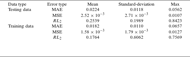
Statistics of reconstruction errors for the ML model trained on 4-D thermal sheath data, detailing the reconstruction errors of IEAD compared with the original data for both testing and training dataset.

Data preparation of the ML model, showing the procedure for (a) single-species and (b) multi-species.

While requirements (i) and (iii) should be fixed for all species, this is not the case for requirement (ii). To satisfy requirement (ii), the maxima energy bin for the
 $j{\mathrm{th}}$
species in a given input vector is computed according to (A17). The first term of (A17) accounts for the thermal distribution of the ions’ source, with an average energy distribution of
 $\frac {3}{2} T_i$
, the latter is multiplied by 3 to account for the high energy portion of the distribution, and then multiplied by 2 as a factor of safety. The last term of (A17) accounts for the energy gained by an ion located at the centre of the domain as it is accelerated by the RF E-field at its peak voltage
 $V_{\mathrm{pp}}$
, with a value estimated as
 $2 Z^j V_{\mathrm{pp}}$
and multiplied by a safety factor of 0.25.
 \begin{align} \frac {e \phi _w }{K_B T_e} &= -\frac {1}{2} \ln\left ( \frac {m_i/m_e}{2\pi (1+ {T_i}/{T_e})} \right )\!,\\[-2pt]\nonumber \end{align}
 \begin{align} E_{\mathrm{max}}^j &= 9 T_i^j + 2.25 Z^j \left ( \phi _w^j +V_{\mathrm{pp}} \right )\!. \end{align}
The middle term of (A17) given by
 $(2.25 Z^j \phi _w^j)$
accounts for the total energy gained by an ion located in the middle of the domain as it is accelerated by the floating wall potential
 $\phi _w$
of the thermal plasma sheath given by (A16). A factor of 1.7 was added to account for the plasma pre-sheath. For simplicity, the factor 2.25 was used instead.
Appendix B. Statistics of prediction errors for the ML model
Statistics of reconstruction errors for the ML model trained on the single-species RF sheath dataset. The table reports reconstruction errors of the IEAD compared with the original data for both the training and testing datasets. It includes results for different model variants: the baseline model, the multi-fidelity (MF) model, the data-augmented (DA) model and the combined MF + DA model. The ‘last step’ variant shows the reconstruction error when using only the original data (without augmentation).

Appendix C. ML models hyper-parameters details
Summary of hyper-parameters used to train the ML model on the single-species, thermal sheath dataset.

 $^\dagger$
Kingma & Ba (Reference Kingma and Ba2014).
Appendix D. Additional results
Summary of hyper-parameters used to train the multi-fidelity and the data-augmented (DA) models on the single-species, RF sheath dataset. Values inside brackets show the value when DA model is included.

 $^\ddagger$
Kingma & Ba (Reference Kingma and Ba2014).
Summary of hyper-parameters used to train the multi-species RF sheath dataset.

Examples of three representative IEAD predictions for a single-species RF sheath. (a) Good illustrates excellent agreement. (b) Average demonstrates moderate deviations while maintaining the overall distribution shape. (c) Poor corresponds to a poor prediction. In each example, the first row compares the reference distribution from hPIC2 (left) with the surrogate predictions from the baseline, data-augmented (DA), multi-fidelity (MF) and combined DA+MF models. The second row shows the corresponding residual error distributions for each model.












 Open access

