









1. Introduction
With the rapid advancement of modern science and technology, many scientific disciplines, such as genetic engineering, signal processing, and machine learning, are increasingly confronted with the challenge of analyzing high-dimensional data. This trend has spurred a growing interest in the study of large-dimensional random matrices, which serve as powerful tools for modeling and understanding the structure of such data. In the theory of large-dimensional random matrices, two central concepts are the empirical spectral distribution (ESD) and the limiting spectral distribution (LSD), which are crucial for characterizing the asymptotic behavior of eigenvalues. Let
 $M \in {{\mathbb R}^{p \times p}}$
be a symmetric square matrix with real eigenvalues
 $\{ {\lambda _j}\} _{j=1}^p$
. The ESD of
 $M$
, denoted by
 ${F^M}$
, is defined as the cumulative distribution function:
 $F^M(x) = \#\{j \in \{1, \ldots, p\} \colon \lambda_j \leq x\}/p$
, where
 $\# \{ \cdot \} $
denotes the cardinality of the set. The LSD is defined as the weak limit of the sequence of ESDs.
The well-known semicircle law and Marčenko–Pastur law, established in [Reference Marčenko and Pastur7, Reference Wigner8], respectively, are foundational results in random matrix theory. In this paper, we aim to derive the LSD for a matrix of the form
 \begin{equation} \boldsymbol{\Omega}=\boldsymbol{\Omega}(\mathbf{X})=\frac{(\mathbf{X}\mathbf{P}_1+\mathbf{A})(\mathbf{X}\mathbf{P}_1+\mathbf{A})'}{n_1}\bigg(\frac{\mathbf{X}\mathbf{P}_2\mathbf{X}'}{n_2}\bigg)^{-1},\end{equation}
where
 $\mathbf{P}_1$
and
 $\mathbf{P}_2$
are projection matrices satisfying
 $\mathrm{rank}(\mathbf{P}_1)=n_1$
,
 $\mathrm{rank}(\mathbf{P}_2)=n_2$
, and
 $\mathbf{P}_1\mathbf{P}_2=0$
(refer to Theorem 1 for additional details). The matrix
 $\mathbf{X}\mathbf{P}_2\mathbf{X}'$
may be singular under the finite second moment condition. Therefore, the inverse in this paper is chosen as the Moore–Penrose inverse.
We now discuss the motivation for studying the matrix model
 $\boldsymbol{\Omega}$
. A primary reason lies in its close connection to canonical correlation analysis (CCA), where such matrices frequently arise. CCA is a classical statistical technique used to quantify the association between two sets of random variables. Specifically, let
 $\mathbf{x}= \lbrace x_1,\ldots,x_{p_1}\rbrace$
and
 $\mathbf{y} = \lbrace y_1,\ldots,y_{p_2}\rbrace$
denote two random vectors, where
 $p_1 \leq p_2$
. Suppose we have n observations for each of the
 $p_1 + p_2$
variables, which are arranged into the random matrices
 $\mathbf{X} = (X_{ij})_{p_1\times n}$
and
 $\mathbf{Y} = (Y_{ij})_{p_2\times n}$
, respectively. CCA aims to identify linear combinations
 $\mathbf{a}'\mathbf{x}$
and
 $\mathbf{c}'\mathbf{y}$
that are maximally correlated, i.e. it seeks to maximize
 \begin{align*}r=\mathrm{Corr}(\mathbf{a}'\mathbf{x},\mathbf{c}'\mathbf{y}) =\frac{\mathbf{a}'\boldsymbol{\Sigma_{xy}}\mathbf{c}}{\sqrt{\mathbf{a}'\boldsymbol{\Sigma_{xx}}\mathbf{a}}\sqrt{\mathbf{c}'\boldsymbol{\Sigma_{yy}}\mathbf{c}}\,},\end{align*}
where
 $\boldsymbol{\Sigma_{xx}}$
and
 $\boldsymbol{\Sigma_{yy}}$
denote the population covariance matrices of
 $\mathbf{x}$
and
 $\mathbf{y}$
, respectively, and
 $\boldsymbol{\Sigma_{xy}}$
is the population covariance matrix between
 $\mathbf{x}$
and
 $\mathbf{y}$
. After obtaining the maximal canonical correlation
 $r_1$
along with the corresponding linear combination vectors
 $\mathbf{a}_1$
and
 $\mathbf{c}_1$
, CCA proceeds to identify a second pair of linear combinations,
 $\mathbf{a}'_2\mathbf{x}$
and
 $\mathbf{c}'_2\mathbf{y}$
, that maximize the correlation subject to being uncorrelated with the first pair,
 $\mathbf{a}'_1\mathbf{x}$
and
 $\mathbf{c}'_1\mathbf{y}$
. This iterative procedure continues until all canonical correlation coefficients
 $r_1 ,\ldots, r_{p_1}$
are obtained. When the population covariance matrices are replaced by their sample counterparts, the canonical correlations
 $r_1,\ldots,r_{p_1}$
correspond to the roots of the determinant equation
 \begin{equation} \mathrm{det}\big(\mathbf{S}_{xy}\mathbf{S}_{y}^{-1}\mathbf{S}_{xy}'-r^2\mathbf{S}_{x}\big)=0,\end{equation}
where
 $\mathbf{S}_{x}=\mathbf{X}\mathbf{X}'/n$
,
 $\mathbf{S}_{y}=\mathbf{Y}\mathbf{Y}'/n$
, and
 $\mathbf{S}_{xy}=\mathbf{X}\mathbf{Y}'/n$
. For further details, see [Reference Yang and Pan9]. Define
 $\mathbf{P}_y=\mathbf{Y}'(\mathbf{Y}\mathbf{Y}')^{-1}\mathbf{Y}$
; (2) can then be simplified to the form
 $\mathrm{det}(\mathbf{X}\mathbf{P}_y\mathbf{X}'-r^2\mathbf{X}\mathbf{X}')=0$
. Of particular relevance to our work is the unified framework proposed in [Reference Han, Pan and Yang4], in which the canonical correlation coefficients, r, are transformed via
 $\lambda={r^2}/{(1-r^2)}$
. Under the condition
 $\lim\inf_{n \to \infty}{n}/{(p_1+p_2)}>1$
, the canonical correlation roots are shown to satisfy the determinant equation
 $\mathrm{det}(\mathbf{X}\mathbf{P}_y\mathbf{X}'-\lambda\mathbf{X}(\mathbf{I}-\mathbf{P}_y)\mathbf{X}')=0$
. The matrix of interest in our analysis thus takes the form
 \begin{equation} (\mathbf{X}(\mathbf{I}-\mathbf{P}_y)\mathbf{X}')^{-1}\mathbf{X}\mathbf{P}_y\mathbf{X}'.\end{equation}
When
 $\mathbf{X}$
and
 $\mathbf{Y}$
are independent, [Reference Han, Pan and Yang4] proposed a unified matrix model
 \begin{align*}\boldsymbol{\Omega}_0=(\mathbf{X}\mathbf{U}_2\mathbf{U}_2'\mathbf{X}')^{-1}\mathbf{X}\mathbf{U}_1\mathbf{U}_1'\mathbf{X}',\end{align*}
where
 $\mathbf{U}_1'\mathbf{U}_1=\mathbf{I}$
,
 $\mathbf{U}_2'\mathbf{U}_2=\mathbf{I}$
, and
 $\mathbf{U}_1'\mathbf{U}_2=0$
.
Consider the case where
 $\mathbf{X}$
and
 $\mathbf{Y}$
are not independent, and let
 $\boldsymbol{\Lambda}$
denote the correlation structure between them. This implies that a portion of the variance in
 $\mathbf{X}$
can be explained by
 $\mathbf{Y}$
through
 $\boldsymbol{\Lambda}$
. However, there remains a component of
 $\mathbf{X}$
’s variance that is not captured by
 $\mathbf{Y}$
, which may be attributed to other factors that are independent of
 $\mathbf{Y}$
. To reflect this, we assume that
 $\mathbf{X}$
and
 $\mathbf{Y}$
follow the structure
 $\mathbf{X}=\boldsymbol{\Lambda}\mathbf{Y}+\boldsymbol{\Gamma}\mathbf{W}$
, where
 $\boldsymbol{\Gamma}$
is the square root matrix of
 $\mathbf{I}_p-\boldsymbol{\Lambda}\boldsymbol{\Lambda}'$
, and
 $\mathbf{W}$
is a
 $p \times n$
matrix independent of
 $\mathbf{Y}$
. Equation (3) can be transformed into the following form:
 \begin{align*} &(\boldsymbol{\Lambda}\mathbf{Y}\mathbf{P}_y+\boldsymbol{\Gamma}\mathbf{W}\mathbf{P}_y) (\boldsymbol{\Lambda}\mathbf{Y}\mathbf{P}_y+\boldsymbol{\Gamma}\mathbf{W}\mathbf{P}_y)' [(\boldsymbol{\Gamma}\mathbf{W}(\mathbf{I}-\mathbf{P}_y))(\boldsymbol{\Gamma}\mathbf{W}(\mathbf{I}-\mathbf{P}_y))']^{-1} \\ &\qquad= (\boldsymbol{\Gamma}^{-1}\boldsymbol{\Lambda}\mathbf{Y}\mathbf{P}_y+\mathbf{W}\mathbf{P}_y) (\boldsymbol{\Gamma}^{-1}\boldsymbol{\Lambda}\mathbf{Y}\mathbf{P}_y+\mathbf{W}\mathbf{P}_y)' [(\mathbf{W}(\mathbf{I}-\mathbf{P}_y))(\mathbf{W}(\mathbf{I}-\mathbf{P}_y))']^{-1}.\end{align*}
Motivated by this, and by considering
 $\boldsymbol{\Gamma}^{-1}\boldsymbol{\Lambda}\mathbf{Y}\mathbf{P}_y$
,
 $\mathbf{W}\mathbf{P}_y$
, and
 $\mathbf{W}(\mathbf{I}-\mathbf{P}_y)$
as
 $\mathbf{A}$
,
 $\mathbf{X}\mathbf{P}_1$
, and
 $\mathbf{X}\mathbf{P}_2$
, respectively, we introduce a novel matrix model as given in (1), which we term the ‘noncentral unified model’ (see Theorem 1 for a detailed formulation). Thus, the study of traditional canonical correlation analysis is equivalent to studying the spectrum of this matrix.
As expected, when the underlying population is Gaussian, the matrix
 $\boldsymbol{\Omega}$
reduces to a noncentral Fisher matrix, whose LSD was established in [Reference Zhang, Bai and Hu11]. In the absence of the Gaussian assumption, we adopt an interpolation-based Gaussian comparison technique, following the methodology of [Reference Li, Han and Yang6], and rigorously demonstrate that the LSD remains the same as in the Gaussian case. This model extends beyond the classical framework of CCA, providing a unified tool applicable to a wide range of multivariate statistical inference problems, and thus holds considerable theoretical and practical importance.
We now briefly review the relevant literature. As the dimensions
 $p_1$
and
 $p_2$
grow on the same order as the sample size n, the classical consistency results for CCA no longer hold. This phenomenon has attracted significant attention and has led to the development of high-dimensional CCA methodologies. [Reference Yang and Pan9] derived the LSD of the sample canonical correlation matrix. Building on this, [Reference Yang and Pan10] proved a central limit theorem for its linear spectral statistics, and [Reference Bao, Hu, Pan and Zhou2] investigated the asymptotic behavior of its spiked eigenvalues. Particularly inspiring to our work, [Reference Li, Han and Yang6] obtained the LSD for
 $\boldsymbol{\Omega}_0$
using the Gaussian comparison method under only a finite second moment condition, while [Reference Han, Pan and Yang4] established the Tracy–Widom distribution for its largest eigenvalue.
The remainder of this paper is structured as follows. In Section 2, we formally state the main theoretical results. Section 3 is devoted to presenting the preliminary definitions and results required for the subsequent analysis. Section 4 details the technical methods and provides a rigorous proof of the main theorem. In Section 5, we conduct simulation studies to demonstrate the validity of our theoretical findings. Finally, the appendix provides additional lemmas to support the main results.
For notational convenience, we use
 $[N]=\lbrace 1,\ldots,N\rbrace$
for any
 $N\in\mathbb{N}^+$
. The symbol
 $\xrightarrow{\mathrm{w}}$
denotes weak convergence. The indicator function is denoted by
 $\mathbf{1}\lbrace\cdot\rbrace$
. We use c to represent a generic constant whose value may vary from line to line. When a constant depends on an additional parameter
 $\alpha$
, we write it as
 $c_{\alpha}$
.
2. Main result
We begin by introducing the assumptions that underpin the high-dimensional setting. Subsequently, we derive the Stieltjes transform (ST) of the LSD of the matrix
 $\boldsymbol{\Omega}$
.
Theorem 1. Assume that
-
(i)
 $\mathbf{X}=(X_{ij})$
,
$i\in[p]$
,
$j\in [n]$
, where
$X_{ij}$
are independent and identically distributed (i.i.d.) with
$\mathbb{E}X_{11}=0$
and
$\mathbb{E}X_{11}^2=1$
.
-
(ii)
$\mathbf{P}_1,\mathbf{P}_2\in\mathbb{R}^{n\times n}$
are projection matrices satisfying
$\mathrm{rank}(\mathbf{P}_1)=n_1$
,
$\mathrm{rank}(\mathbf{P}_2)=n_2$
, and
$\mathbf{P}_1\mathbf{P}_2=0$
. Additionally, when
$\mathbf{P}_1$
and
$\mathbf{P}_2$
are random matrices, they are independent of
$\mathbf{X}$
. -
(iii) As
$\min\{p,n_1,n_2\}\to\infty$
,
$p/n_1\rightarrow c_1\in(0,\infty)$
and
$p/n_2\rightarrow c_2\in(0,1)$
. -
(iv)
$\mathbf{A}$
is a
$p\times n$
nonrandom matrix and the ESD
$H_n $
of
$\mathbf{A}\mathbf{A}'/n_1$
satisfies
$H_n\xrightarrow{\mathrm{w}}{H}$
, where H is a nonrandom probability measure.


Then, as
 $n\to \infty$
, the ESD of
 $\boldsymbol{\Omega}$
converges almost surely to a nonrandom distribution, denoted by F, whose ST s(z) is the unique solution in the set
 $\lbrace zs(z)\in\mathbb{C}^{+}\rbrace$
to the equation
 \begin{equation} s(z) = \int\frac{{\mathrm{d}} H(t)}{ \dfrac{t}{1+(c_1+c_2z)s(z)}+\dfrac{1-c_1}{1+c_2zs(z)}-\dfrac{z(1+(c_1+c_2z)s(z))}{1+c_2zs(z)}\,}, \quad z\in\mathbb{C}^{+}. \end{equation}
In particular, if
 $c_1>1$
, F has a point mass
 $1-{1}/{c_1}$
at the origin.
Remark 1. The result of our theorem indicates that the LSD of the matrix
 $\boldsymbol{\Omega}$
coincides with that of the noncentral F-matrix. (The LSD of the noncentral F-matrix is presented in [Reference Zhang, Bai and Hu11].) While this conclusion is straightforward in the Gaussian setting, a detailed justification for the non-Gaussian case is presented in Section 4.2.
Remark 2. This result generalizes the main conclusion of [Reference Li, Han and Yang6], which established that the LSD of
 $\boldsymbol{\Omega}$
matches that of a central F-matrix in the special case where
 $\mathbf{A}=\mathbf{0}$
. By allowing
 $\mathbf{A}\neq\mathbf{0}$
, we extend the analysis to the noncentral case, thereby broadening the applicability of the original framework.
3. Preparations for the proof
We begin by defining
 $\mathbf{S}_1={(\mathbf{X}\mathbf{P}_1+\mathbf{A})(\mathbf{X}\mathbf{P}_1+\mathbf{A})'}/{n_1}$
and
 $\mathbf{S}_2={\mathbf{X}\mathbf{P}_2\mathbf{X}'}/{n_2}$
. To complete the proof of Theorem 1, it is sufficient to show the almost sure convergence of
 $F^{\mathbf{S}_1\mathbf{S}_2^{-1}}$
.
3.1. Introduction of matrix
$\mathbf{B}$

Consider the Beta-type matrix
 $\mathbf{B}=\mathbf{B}(\mathbf{X})=\mathbf{S}_2(\mathbf{S}_1+\mathbf{S}_2)^{-1}$
. Inspired by [Reference Li, Han and Yang6], we transform the analysis from
 $\mathbf{S}_1\mathbf{S}_2^{-1}$
to the Beta-type matrix
 $\mathbf{B}$
. We first assert that proving the almost sure convergence of the ESD of
 $\mathbf{B}$
is sufficient to establish Theorem 1, and we now proceed to justify this assertion. Let
 $Q_c$
denote the standard Marčenko–Pastur distribution with support on the interval
 $[(1-\sqrt{c})^2,(1+\sqrt{c})^2]$
. It is well known that the ESD of
 $\mathbf{S}_2$
converges almost surely to
 $Q_{c_2}$
as
 $p \to \infty$
. Therefore, we obtain
 \begin{equation} 1 - \frac{1}{p}\mathrm{rank}(\mathbf{S}_2) \leq \frac{1}{p}\#\bigg\lbrace \mathrm{eigenvalues\ of}\ \mathbf{S}_2\ \mathrm{smaller\ than}\ \frac{(1-\sqrt{c_2})^2}{2}\bigg\rbrace \rightarrow 0 \quad \text{a.s.} .\end{equation}
Suppose that
 $\mathbf{S}_2^{{1}/{2}}$
denotes the (nonnegative definite) square root of
 $\mathbf{S}_2$
, and let
 $\mathbf{S}_2^{-{1}/{2}}$
be its Moore–Penrose inverse. Then, the product
 $\mathbf{S}_2^{-{1}/{2}}\mathbf{S}_2\mathbf{S}_2^{-{1}/{2}}=\mathbf{S}_2^{-1}\mathbf{S}_2$
is a projection matrix. The following identity plays a key role in our analysis:
 \begin{align*} & \mathbf{S}_2^{{1}/{2}}(\mathbf{S}_2+\mathbf{S}_1)^{-1}\mathbf{S}_2^{{1}/{2}} - \big(\mathbf{I}+\mathbf{S}_2^{-{1}/{2}}\mathbf{S}_1\mathbf{S}_2^{-{1}/{2}}\big)^{-1} \\ & \qquad = \big(\mathbf{S}_2^{-{1}/{2}}(\mathbf{S}_2+\mathbf{S}_1)^{-1}\mathbf{S}_2^{-{1}/{2}}\big)^{-1} - \big(\mathbf{I}+\mathbf{S}_2^{-{1}/{2}}\mathbf{S}_1\mathbf{S}_2^{-{1}/{2}}\big)^{-1} \\ & \qquad = \big(\mathbf{S}_2^{-{1}/{2}}\mathbf{S}_2\mathbf{S}_2^{-{1}/{2}} \big(\mathbf{I}+\mathbf{S}_2^{-{1}/{2}}\mathbf{S}_1\mathbf{S}_2^{-{1}/{2}}\big)\big)^{-1} - \big(\mathbf{I}+\mathbf{S}_2^{-{1}/{2}}\mathbf{S}_1\mathbf{S}_2^{-{1}/{2}}\big)^{-1} \\ & \qquad = \big(\mathbf{I}+\mathbf{S}_2^{-{1}/{2}}\mathbf{S}_1\mathbf{S}_2^{-{1}/{2}}\big)^{-1} \big(\mathbf{S}_2^{-1}\mathbf{S}_2-\mathbf{I}\big).\end{align*}
In conjunction with Lemma 1 and (5), this implies that
 \begin{equation*} \big\|F^{\mathbf{S}_2^{{1}/{2}}(\mathbf{S}_2+\mathbf{S}_1)^{-1}\mathbf{S}_2^{{1}/{2}}} - F^{\big(\mathbf{I}+\mathbf{S}_2^{-{1}/{2}}\mathbf{S}_1\mathbf{S}_2^{-{1}/{2}}\big)^{-1}}\big\| \leq \frac{1}{p}\mathrm{rank}(\mathbf{S}_2^{-1}\mathbf{S}_2-\mathbf{I}) \rightarrow 0, \quad \text{a.s.}\end{equation*}
Noticing that
 $F^{\mathbf{S}_2^{-{1}/{2}}\mathbf{S}_1\mathbf{S}_2^{-{1}/{2}}}=F^{\mathbf{S}_2^{-1}\mathbf{S}_1}$
and
 $F^{\mathbf{B}}=F^{\mathbf{S}_2^{{1}/{2}}(\mathbf{S}_2+\mathbf{S}_1)^{-1}\mathbf{S}_2^{{1}/{2}}}$
, and using the fact that if
 $\lambda$
is an eigenvalue of
 $(\mathbf{I}+\mathbf{S}_2^{-{1}/{2}}\mathbf{S}_1\mathbf{S}_2^{-{1}/{2}})^{-1}$
then
 $\lambda^{-1}-1$
is an eigenvalue of
 $\mathbf{S}_2^{-{1}/{2}}\mathbf{S}_1\mathbf{S}_2^{-{1}/{2}}$
, we deduce the stated claim. Consequently, it suffices to analyze the convergence behavior of
 $F^{\mathbf{B}}$
. Due to the asymmetry of
 $\mathbf{B}$
, we introduce an auxiliary matrix for technical convenience:
 \begin{align*}\underline{\mathbf{B}}=\underline{\mathbf{B}}(\mathbf{X})=\frac{1}{n_2}\mathbf{U}_2'\mathbf{X}'(\mathbf{S}_1+\mathbf{S}_2)^{-1}\mathbf{X}\mathbf{U}_2,\end{align*}
where
 $\mathbf{U}_2$
is an
 $n\times n_2$
isometric matrix satisfying
 $\mathbf{P}_2=\mathbf{U}_2\mathbf{U}_2'$
and
 $\mathbf{U}_2'\mathbf{U}_2=\mathbf{I}$
. Clearly,
 $\mathbf{B}$
and
 $\underline{\mathbf{B}}$
share the same nonzero eigenvalues, differing only by
 $(n_2-p)$
zero eigenvalues, i.e.
 \begin{align*}F^{\underline{\mathbf{B}}}(x)=\frac{p}{n_2}F^{\mathbf{B}}(x)+\frac{n_2-p}{n_2}\mathbf{1}\lbrace x\in[0,\infty)\rbrace.\end{align*}
3.2. Introduction of perturbation matrix
To ensure the invertibility of the matrix
 $(\mathbf{S}_1+\mathbf{S}_2)$
, we introduce a perturbed matrix
 \begin{align*}\underline{\mathbf{B}}_t(\mathbf{X})=\frac{1}{n_2}\mathbf{U}_2'\mathbf{X}'(\mathbf{S}_1+\mathbf{S}_2+t\mathbf{I})^{-1}\mathbf{X}\mathbf{U}_2,\end{align*}
where t is a small positive constant. The tightness of the ESD
 $F^{\underline{\mathbf{B}}_t}$
follows readily from the observation that the eigenvalues of
 $\underline{\mathbf{B}}_t$
are bounded by 1, which implies that, for any constant
 $K > 1$
,
 \begin{align*}\int_{\lambda>K}{\mathrm{d}} F^{\underline{\mathbf{B}}_t}=\frac{1}{n_2}\sum_{i=1}^{n_2}\mathbf{1}\lbrace\lambda_i>K\rbrace=0.\end{align*}
We express the spectral decomposition of
 $(\mathbf{S}_1+\mathbf{S}_2)$
as
 $\mathbf{S}_1+\mathbf{S}_2=\sum_{i=1}^{p}\mu_{i}\mathbf{u}_i\mathbf{u}_i'$
, where
 $\mu_{i}$
and
 $\mathbf{u}_i$
denote the respective eigenvalues and corresponding orthonormal eigenvectors. According to the definition of the Moore–Penrose inverse, we have
 \begin{align*} (\mathbf{S}_1+\mathbf{S}_2)((\mathbf{S}_1+\mathbf{S}_2+t\mathbf{I})^{-1}-(\mathbf{S}_1+\mathbf{S}_2)^{-1}) & = \sum_{i=1}^{p}\mathbf{1}\lbrace\mu_{i}>0\rbrace\mu_{i}\bigg(\frac{1}{\mu_{i}+t}-\frac{1}{\mu_{i}}\bigg) \mathbf{u}_i\mathbf{u}_i' \\ & = \sum_{i=1}^{p}\mathbf{1}\lbrace\mu_{i}>0\rbrace\frac{-t}{\mu_i+t}\mathbf{u}_i\mathbf{u}_i'.\end{align*}
Combining this with Lemma 2, we have
 \begin{align} L^3(F^{\underline{\mathbf{B}}},F^{\underline{\mathbf{B}}_t}) & \leq \frac{1}{n_2}\mathrm{tr}(\underline{\mathbf{B}}_t-\underline{\mathbf{B}})^2 \nonumber \\ & \leq \frac{1}{n_2}\mathrm{tr}\big(\mathbf{S}_2\big((\mathbf{S}_1+\mathbf{S}_2+t\mathbf{I})^{-1} - (\mathbf{S}_1+\mathbf{S}_2)^{-1}\big)\big)^2 \nonumber \\ & \leq \frac{1}{n_2}\mathrm{tr}\big((\mathbf{S}_1+\mathbf{S}_2)\big((\mathbf{S}_1+\mathbf{S}_2+t\mathbf{I})^{-1} - (\mathbf{S}_1+\mathbf{S}_2)^{-1}\big)\big)^2 \nonumber \\ & \leq \frac{t^2}{n_2}\mathrm{tr}(\mathbf{S}_1+\mathbf{S}_2+t\mathbf{I})^{-2} \leq \frac{t^2}{n_2}\mathrm{tr}(\mathbf{S}_2+t\mathbf{I})^{-2}. \end{align}
Notice that the ESD of
 $\mathbf{S}_2$
converges almost surely to
 $Q_{c_2}$
as
 $p \to \infty$
, so we have
 \begin{equation*} \frac{1}{n_2}\mathrm{tr}(\mathbf{S}_2+t\mathbf{I})^{-2} = \frac{p}{n_2}\int\frac{1}{(\lambda+t)^2}\,{\mathrm{d}} F^{\mathbf{S}_2} \xrightarrow{\mathrm{a.s.}} c_2\int\frac{1}{(\lambda+t)^2}\,{\mathrm{d}} Q_{c_2} \leq \frac{c_2}{(1-\sqrt{c_2})^4},\end{equation*}
which together with (6) implies that
 $\lim_{t\to0}\lim_{n\to\infty}L(F^{\underline{\mathbf{B}}},F^{\underline{\mathbf{B}}_t})=0$
, almost surely (a.s.). Therefore, it suffices to prove the almost sure convergence of
 $F^{\underline{\mathbf{B}}_t}$
in the following sections.
3.3. Truncation of matrix
$\mathbf{A}$

Let
 $\mathbf{A}/{\sqrt{n_1}}$
admit the singular value decomposition
 $\mathbf{A}/{\sqrt{n_1}}=\mathbf{U}\boldsymbol{\Lambda}\mathbf{V}$
, where
 $\mathbf{U}$
and
 $\mathbf{V}$
are orthogonal matrices, and
 $\boldsymbol{\Lambda}$
is a diagonal matrix containing the singular values
 $s_i$
. Define a truncated version
 $\mathbf{A}_{\alpha}/{\sqrt{n_1}}$
as
 $\mathbf{A}_{\alpha}/{\sqrt{n_1}}=\mathbf{U}\boldsymbol{\Lambda}_{\alpha}\mathbf{V}$
, where
 $\boldsymbol{\Lambda}_{\alpha}$
is obtained from
 $\boldsymbol{\Lambda}$
by replacing each singular value
 $s_i$
with
 $s_i\mathbf{1}\{s_i\leq\alpha\}$
for some threshold
 $\alpha >0$
. Let
 $\mathbf{Q}$
be an arbitrary
 $p \times n$
matrix, and
 $\mathbf{R}$
be an arbitrary
 $p \times p$
matrix. Then the perturbed matrix
 $\underline{\mathbf{B}}_t$
can be expressed in the form
 \begin{align*}\mathbf{R}\bigg[\bigg(\frac{1}{\sqrt{n_1}\,}\mathbf{A}+\mathbf{Q}\bigg)\bigg(\frac{1}{\sqrt{n_1}\,}\mathbf{A}+\mathbf{Q}\bigg)'+\mathbf{R}+t\mathbf{I}\bigg]^{-1}.\end{align*}
Using the rank inequality, we calculate
 \begin{align*} & \big\|F^{\mathbf{R}[(\mathbf{A}/{\sqrt{n_1}}+\mathbf{Q})(\mathbf{A}/{\sqrt{n_1}}+\mathbf{Q})'+\mathbf{R}+t\mathbf{I}]^{-1}} - F^{\mathbf{R}[(\mathbf{A}_{\alpha}/{\sqrt{n_1}}+\mathbf{Q})(\mathbf{A}_{\alpha}/{\sqrt{n_1}}+\mathbf{Q})'+\mathbf{R}+t\mathbf{I}]^{-1}}\big\|\\ & \qquad \leq \frac{1}{p}\mathrm{rank}\bigg(\bigg[\bigg(\frac{1}{\sqrt{n_1}\,}\mathbf{A}+\mathbf{Q}\bigg) \bigg(\frac{1}{\sqrt{n_1}\,}\mathbf{A}+\mathbf{Q}\bigg)' + \mathbf{R} + t\mathbf{I}\bigg]^{-1} \\ & \qquad\qquad\qquad\quad - \bigg[\bigg(\frac{1}{\sqrt{n_1}\,}\mathbf{A}_{\alpha}+\mathbf{Q}\bigg) \bigg(\frac{1}{\sqrt{n_1}\,}\mathbf{A}_{\alpha}+\mathbf{Q}\bigg)' + \mathbf{R} + t\mathbf{I}\bigg]^{-1}\bigg) \\ & \qquad \leq \frac{1}{p}\mathrm{rank}\bigg[\bigg(\frac{1}{\sqrt{n_1}\,}\mathbf{A}+\mathbf{Q}\bigg) \bigg(\frac{1}{\sqrt{n_1}\,}\mathbf{A}+\mathbf{Q}\bigg)' - \bigg(\frac{1}{\sqrt{n_1}\,}\mathbf{A}_{\alpha}+\mathbf{Q}\bigg) \bigg(\frac{1}{\sqrt{n_1}\,}\mathbf{A}_{\alpha}+\mathbf{Q}\bigg)'\bigg] \\ & \qquad = \frac{1}{p}\mathrm{rank}\bigg[\bigg(\frac{1}{\sqrt{n_1}\,}\mathbf{A}+\mathbf{Q}\bigg) \bigg(\frac{1}{\sqrt{n_1}\,}\mathbf{A}+\mathbf{Q}\bigg)' - \bigg(\frac{1}{\sqrt{n_1}\,}\mathbf{A}+\mathbf{Q}\bigg) \bigg(\frac{1}{\sqrt{n_1}\,}\mathbf{A}_{\alpha}+\mathbf{Q}\bigg)' \\ & \qquad\qquad\qquad\quad + \bigg(\frac{1}{\sqrt{n_1}\,}\mathbf{A}+\mathbf{Q}\bigg) \bigg(\frac{1}{\sqrt{n_1}\,}\mathbf{A}_{\alpha}+\mathbf{Q}\bigg)' - \bigg(\frac{1}{\sqrt{n_1}\,}\mathbf{A}_{\alpha}+\mathbf{Q}\bigg) \bigg(\frac{1}{\sqrt{n_1}\,}\mathbf{A}_{\alpha}+\mathbf{Q}\bigg)'\bigg] \\ & \qquad \leq \frac{2}{p}\mathrm{rank}\bigg(\frac{1}{\sqrt{n_1}\,}\mathbf{A} - \frac{1}{\sqrt{n_1}\,}\mathbf{A}_{\alpha}\bigg) \\ & \qquad \leq \frac{2}{p}\sum_{i=1}^{p}\mathbf{1}\{s_i>\alpha\} = \frac{2}{p}\sum_{i=1}^{p}\mathbf{1}\{\lambda_i>\alpha^2\} \xrightarrow{\mathrm{a.s.}} 2H{(\alpha^2,\infty)},\end{align*}
where the
 $\lambda_i$
are the eigenvalues of
 $\mathbf{A}\mathbf{A}'/{n_1}$
, i.e.
 $\lambda_i=s_i^2$
. Since H is a probability measure on the nonnegative real line, for any
 $\varepsilon > 0$
there is a constant
 $\tau > 0$
such that
 $H(\lambda_i>\tau) < \varepsilon$
. We choose
 $\alpha^2 > \tau$
; it follows that, as
 $n \to \infty$
,
 \begin{align*}\big\|F^{\mathbf{R}[(\mathbf{A}/{\sqrt{n_1}}+\mathbf{Q})(\mathbf{A}/{\sqrt{n_1}}+\mathbf{Q})'+\mathbf{R}+t\mathbf{I}]^{-1}} -F^{\mathbf{R}[(\mathbf{A}_{\alpha}/{\sqrt{n_1}}+\mathbf{Q})(\mathbf{A}_{\alpha}/{\sqrt{n_1}}+\mathbf{Q})'+\mathbf{R}+t\mathbf{I}]^{-1}}\big\|\xrightarrow{\mathrm{a.s.}} 0.\end{align*}
We can now proceed with the proof under the condition that the spectral norm of
 $\mathbf{A}\mathbf{A}'/{n_1}$
is bounded.
3.4. Truncation, centralization, and renormalization
Let
 $\widetilde{X}_{ij}=X_{ij}\mathbf{1}\lbrace|X_{ij}|<\sqrt{n}\eta\rbrace$
and
 $\widehat{X}_{ij}=\widetilde{X}_{ij}-\mathbb{E}\widetilde{X}_{11}$
, where
 ${\eta}$
is any fixed constant. We write
 $\widetilde{\mathbf{X}}=(\widetilde{X}_{ij})_{p\times n}$
and
 $\widehat{\mathbf{X}}=(\widehat{X}_{ij})_{p\times n}$
. Analogously, we let
 \begin{align*} \widetilde{\underline{\mathbf{B}}}_t & = \frac{1}{n_2}\mathbf{U}_2'\widetilde{\mathbf{X}}'\bigg(\frac{1}{n_1} (\widetilde{\mathbf{X}}\mathbf{P}_1+\mathbf{A})(\widetilde{\mathbf{X}}\mathbf{P}_1+\mathbf{A})' + \frac{1}{n_2}\widetilde{\mathbf{X}}\mathbf{P}_2\widetilde{\mathbf{X}}' + t\mathbf{I}\bigg)^{-1} \widetilde{\mathbf{X}}\mathbf{U}_2, \\ \widehat{\underline{\mathbf{B}}}_t & = \frac{1}{n_2}\mathbf{U}_2'\widehat{\mathbf{X}}'\bigg(\frac{1}{n_1} (\widehat{\mathbf{X}}\mathbf{P}_1+\mathbf{A})(\widehat{\mathbf{X}}\mathbf{P}_1+\mathbf{A})' + \frac{1}{n_2}\widehat{\mathbf{X}}\mathbf{P}_2\widehat{\mathbf{X}}' + t\mathbf{I}\bigg)^{-1} \widehat{\mathbf{X}}\mathbf{U}_2.\end{align*}
By Lemma 1, we have
 \begin{align*} \|F^{\underline{\mathbf{B}}_t}-F^{\widetilde{\underline{\mathbf{B}}}_t}\| & \leq \frac{1}{n_2}\mathrm{rank}({\underline{\mathbf{B}}}_t-{\widetilde{\underline{\mathbf{B}}}}_t) \\ &\leq \frac{2}{n_2}\text{rank} \left( \mathbf{X}-\widetilde{\mathbf{X}}\right)\\ & \quad + \frac{1}{n_2}\mathrm{rank}\bigg\lbrace \bigg(\frac{\mathbf{X}\mathbf{P}_1\mathbf{X}' + \mathbf{A}\mathbf{P}_1\mathbf{X}' + \mathbf{X}\mathbf{P}_1\mathbf{A}' + \mathbf{A}\mathbf{A}'}{n_1} + \frac{\mathbf{X}\mathbf{P}_2\mathbf{X}'}{n_2} + t\mathbf{I}\bigg)^{-1} \\ & \qquad\qquad\qquad - \bigg(\frac{\widetilde{\mathbf{X}}\mathbf{P}_1\widetilde{\mathbf{X}}' + \mathbf{A}\mathbf{P}_1\widetilde{\mathbf{X}}' + \widetilde{\mathbf{X}}\mathbf{P}_1\mathbf{A}' + \mathbf{A}\mathbf{A}'}{n_1} + \frac{\widetilde{\mathbf{X}}\mathbf{P}_2\widetilde{\mathbf{X}}'}{n_2} + t\mathbf{I}\bigg)^{-1}\bigg\rbrace \\ & \leq \frac{2}{n_2}\mathrm{rank}(\mathbf{X}-\widetilde{\mathbf{X}}) \\ & \quad + \frac{1}{n_2}\mathrm{rank}\bigg( \frac{1}{n_1}(\mathbf{X}\mathbf{P}_1\mathbf{X}'-\widetilde{\mathbf{X}}\mathbf{P}_1\widetilde{\mathbf{X}}') + \frac{1}{n_2}(\mathbf{X}\mathbf{P}_2\mathbf{X}' - \widetilde{\mathbf{X}}\mathbf{P}_2\widetilde{\mathbf{X}}') \\ & \qquad\qquad\qquad + \frac{1}{n_1}\mathbf{A}\mathbf{P}_1(\mathbf{X}-\widetilde{\mathbf{X}})' + \frac{1}{n_1}(\mathbf{X}-\widetilde{\mathbf{X}})\mathbf{P}_1\mathbf{A}'\bigg) \\ & \leq \frac{4}{n_2}\mathrm{rank}(\mathbf{X}-\widetilde{\mathbf{X}}) + \frac{1}{n_2}\mathrm{rank}\bigg( \frac{\mathbf{X}\mathbf{P}_1\mathbf{X}'-\widetilde{\mathbf{X}}\mathbf{P}_1\widetilde{\mathbf{X}}'}{n_1} + \frac{\mathbf{X}\mathbf{P}_2\mathbf{X}'-\widetilde{\mathbf{X}}\mathbf{P}_2\widetilde{\mathbf{X}}'} {n_2}\bigg) \\ & \leq \frac{8}{n_2}\mathrm{rank}(\mathbf{X}-\widetilde{\mathbf{X}}) \leq \frac{8}{n_2}\sum_{ij}\mathbf{1}\lbrace|X_{ij}|\geq\sqrt{n}\eta\rbrace,\end{align*}
where the third inequality is because
 ${\mathbf{M}}_1^{ - 1} - {\mathbf{M}}_2^{ - 1} = {\mathbf{M}}_2^{ - 1}({{\mathbf{M}}_2} - {{\mathbf{M}}_1}){\mathbf{M}}_1^{ - 1}$
holds for any two non-singular matrices
 $\mathbf{M}_1$
and
 $\mathbf{M}_2$
. It follows from Bernstein’s inequality that there exists a universal positive constant c such that
 \begin{align*}\mathbb{P}\Bigg(\frac{1}{n_2}\Bigg|\sum_{ij}\mathbf{1}\lbrace|X_{ij}|\geq\sqrt{n}\eta\rbrace - np\mathbb{E}\mathbf{1}\lbrace|X_{ij}|\geq\sqrt{n}\eta\rbrace\Bigg| \geq \varepsilon\Bigg) \leq {\mathrm{e}}^{-cp} \end{align*}
for all
 $\varepsilon>0$
, which is summable.
Since
 $\mathbb{E}|X_{ij}|^2=1$
and
 ${\mathbb E}|{X_{ij}}{|^2} = {\mathbb E}|{X_{ij}}{|^2}{\bf{1}}\{ |{X_{ij}}| \ge \sqrt n \eta \} + {\mathbb E}|{X_{ij}}{|^2}{\bf{1}}\{ |{X_{ij}}| \lt \sqrt n \eta \} $
, for
 $n \to \infty$
we obtain that
 ${\mathbb E}|{X_{ij}}{|^2}{\bf{1}}\{ |{X_{ij}}| \ge \sqrt n \eta \} \to 0$
. Notice that
 \begin{align*}\mathbb{E}\mathbf{1}\lbrace|X_{ij}|\geq\sqrt{n}\eta\rbrace \leq \frac{\mathbb{E}|X_{ij}|^2\mathbf{1}\lbrace|X_{ij}|\geq\sqrt{n}\eta\rbrace}{\eta^2n} = o\bigg(\frac{1}{n}\bigg).\end{align*}
By the Borel–Cantelli lemma, we have
 $\|F^{\underline{\mathbf{B}}_t}-F^{\widetilde{\underline{\mathbf{B}}}_t}\|\rightarrow0$
a.s. Then, according to Lemma 5, there exists a slowly decreasing sequence
 $\eta_n \to 0$
such that, replacing
 $\eta$
in
 $\widetilde{X}_{ij}$
with
 $\eta_n$
,
 $\|F^{\underline{\mathbf{B}}_t}-F^{\widetilde{\underline{\mathbf{B}}}_t}\| \rightarrow 0$
a.s.
Similarly, we can easily obtain that
 \begin{equation*} \|F^{\widetilde{\underline{\mathbf{B}}}_t}-F^{\widehat{\underline{\mathbf{B}}}_t}\| \leq \frac{8}{n_2}\mathrm{rank}(\mathbb{E}\widetilde{\mathbf{X}}) = \frac{8}{n_2} \rightarrow 0 \ \text{a.s.}\end{equation*}
Let
 \begin{align*}\hat{\sigma}^2 = \mathbb{E}\widehat{X}_{11}^2, \qquad \check{\underline{\mathbf{B}}}_t = \frac{\mathbf{U}_2'\widehat{\mathbf{X}}'}{n_2\hat{\sigma}} \bigg(\frac{(({\widehat{\mathbf{X}}}/{\hat{\sigma}})\mathbf{P}_1 + \mathbf{A})(({\widehat{\mathbf{X}}}/{\hat{\sigma}})\mathbf{P}_1+\mathbf{A})'}{n_1} + \frac{\widehat{\mathbf{X}}\mathbf{P}_2\widehat{\mathbf{X}}'}{n_2\hat{\sigma}^2} + t\mathbf{I}\bigg)^{-1} \frac{\widehat{\mathbf{X}}\mathbf{U}_2}{\hat{\sigma}}.\end{align*}
For any nonnegative definite matrix
 $\mathbf{M}$
and
 $c \in \mathbb{R}^{+}$
, we have
 \begin{align*} \|\mathbf{M}(\mathbf{M}+ct\mathbf{I})^{-1}\| \leq 1, \qquad \|(\mathbf{M}+t\mathbf{I})^{-1}\| \leq \frac{1}{t}, \quad t>0.\end{align*}
Then, by Lemma 2 and the fact that, as
 $n \rightarrow \infty$
,
 \begin{align*} 1 - \hat{\sigma}^2 = \mathbb{E}X_{11}^2\mathbf{1}\lbrace X_{11}\geq\sqrt{n}\eta_n\rbrace + (\mathbb{E}X_{11}\mathbf{1}\lbrace X_{11}\leq\sqrt{n}\eta_n\rbrace)^2 \rightarrow 0.\end{align*}
Also, it is easy to obtain that
 $({1}/{np\hat{\sigma}^2})\sum_{ij}\widehat{X}_{ij}^2 \to 1$
a.s.
It can be shown that
 \begin{align*} L^{3}(F^{\check{\underline{\mathbf{B}}}_t},F^{\widehat{\underline{\mathbf{B}}}_t}) & \leq \frac{1}{n_2}\mathrm{tr}\bigg\lbrace \frac{\widehat{\mathbf{X}}\mathbf{P}_2\widehat{\mathbf{X}}'}{n_2\hat{\sigma}^2} \bigg(\frac{(({\widehat{\mathbf{X}}}/{\hat{\sigma}})\mathbf{P}_1+\mathbf{A}) (({\widehat{\mathbf{X}}}/{\hat{\sigma}})\mathbf{P}_1+\mathbf{A})'}{n_1} + \frac{\widehat{\mathbf{X}}\mathbf{P}_2\widehat{\mathbf{X}}'}{n_2\hat{\sigma}^2} + t\mathbf{I}\bigg)^{-1} \\ & \qquad\qquad - \frac{\widehat{\mathbf{X}}\mathbf{P}_2\widehat{\mathbf{X}}'}{n_2} \bigg(\frac{(\widehat{\mathbf{X}}\mathbf{P}_1+\mathbf{A})(\widehat{\mathbf{X}}\mathbf{P}_1+\mathbf{A})'}{n_1} + \frac{\widehat{\mathbf{X}}\mathbf{P}_2\widehat{\mathbf{X}}'}{n_2} + t\mathbf{I}\bigg)^{-1}\bigg\rbrace^2 \\ & = \frac{1}{n_2}\mathrm{tr}\bigg\lbrace \frac{\widehat{\mathbf{X}}\mathbf{P}_2\widehat{\mathbf{X}}'}{n_2}\bigg[ \bigg(\frac{(\widehat{\mathbf{X}}\mathbf{P}_1+\hat{\sigma}\mathbf{A}) (\widehat{\mathbf{X}}\mathbf{P}_1+\hat{\sigma}\mathbf{A})'}{n_1} + \frac{\widehat{\mathbf{X}}\mathbf{P}_2\widehat{\mathbf{X}}'}{n_2} + \hat{\sigma}^2t\mathbf{I}\bigg)^{-1} \\ & \qquad\qquad - \bigg(\frac{(\widehat{\mathbf{X}}\mathbf{P}_1+\mathbf{A}) (\widehat{\mathbf{X}}\mathbf{P}_1+\mathbf{A})'}{n_1} + \frac{\widehat{\mathbf{X}}\mathbf{P}_2\widehat{\mathbf{X}}'}{n_2} + t\mathbf{I}\bigg)^{-1}\bigg] \bigg\rbrace^2 \\ & = \frac{(1-\hat{\sigma})^2}{n_2}\mathrm{tr}\bigg\lbrace \frac{\widehat{\mathbf{X}}\mathbf{P}_2\widehat{\mathbf{X}}'}{n_2} \bigg(\frac{(\widehat{\mathbf{X}}\mathbf{P}_1+\mathbf{A})(\widehat{\mathbf{X}}\mathbf{P}_1+\mathbf{A})'}{n_1} + \frac{\widehat{\mathbf{X}}\mathbf{P}_2\widehat{\mathbf{X}}'}{n_2} + t\mathbf{I}\bigg)^{-1} \\ & \qquad\qquad\qquad \times \bigg(\frac{\mathbf{A}\mathbf{P}_1\widehat{\mathbf{X}}'}{n_1} + \frac{\widehat{\mathbf{X}}\mathbf{P}_1\mathbf{A}'}{n_1} + (1+\hat{\sigma})\bigg(\frac{\mathbf{A}\mathbf{A}'}{n_1} + t\mathbf{I}\bigg)\bigg) \\ & \qquad\qquad\qquad \times \bigg(\frac{(\widehat{\mathbf{X}}\mathbf{P}_1+\hat{\sigma}\mathbf{A}) (\widehat{\mathbf{X}}\mathbf{P}_1+\hat{\sigma}\mathbf{A})'}{n_1} + \frac{\widehat{\mathbf{X}}\mathbf{P}_2\widehat{\mathbf{X}}'}{n_2} + \hat{\sigma}^2t\mathbf{I}\bigg)^{-1}\bigg\rbrace^2 \\ & \leq \frac{(1-\hat{\sigma})^2}{n_2}\mathrm{tr}\bigg\lbrace \bigg(\frac{\widehat{\mathbf{X}}\mathbf{P}_2\widehat{\mathbf{X}}'}{n_2} + \frac{(\widehat{\mathbf{X}}\mathbf{P}_1+\hat{\sigma}\mathbf{A}) (\widehat{\mathbf{X}}\mathbf{P}_1+\hat{\sigma}\mathbf{A})'}{n_1}\bigg)\\ & \qquad\qquad\qquad \times \bigg(\frac{(\widehat{\mathbf{X}}\mathbf{P}_1+\mathbf{A}) (\widehat{\mathbf{X}}\mathbf{P}_1+\mathbf{A})'}{n_1} + \frac{\widehat{\mathbf{X}}\mathbf{P}_2\widehat{\mathbf{X}}'}{n_2} + t\mathbf{I}\bigg)^{-1} \end{align*}
 \begin{align*} & \qquad\qquad\qquad \times \bigg(\frac{\mathbf{A}\mathbf{P}_1\widehat{\mathbf{X}}'}{n_1} + \frac{\widehat{\mathbf{X}}\mathbf{P}_1\mathbf{A}'}{n_1} + (1+\hat{\sigma})\bigg(\frac{\mathbf{A}\mathbf{A}'}{n_1} + t\mathbf{I}\bigg)\bigg) \\ & \qquad\qquad\qquad \times \bigg(\frac{(\widehat{\mathbf{X}}\mathbf{P}_1+\hat{\sigma}\mathbf{A}) (\widehat{\mathbf{X}}\mathbf{P}_1+\hat{\sigma}\mathbf{A})'}{n_1} + \frac{\widehat{\mathbf{X}}\mathbf{P}_2\widehat{\mathbf{X}}'}{n_2} + \hat{\sigma}^2t\mathbf{I}\bigg)^{-1}\bigg\rbrace^2 \\ & \leq \frac{c(1-\hat{\sigma})^2}{n_2}\mathrm{tr}\bigg\lbrace \bigg(\frac{(\widehat{\mathbf{X}}\mathbf{P}_1+\mathbf{A})(\widehat{\mathbf{X}}\mathbf{P}_1+\mathbf{A})'}{n_1} + \frac{\widehat{\mathbf{X}}\mathbf{P}_2\widehat{\mathbf{X}}'}{n_2} + t\mathbf{I}\bigg)^{-1} \\ & \qquad\qquad\qquad\quad \times \bigg(\frac{\mathbf{A}\mathbf{P}_1\widehat{\mathbf{X}}'}{n_1} + \frac{\widehat{\mathbf{X}}\mathbf{P}_1\mathbf{A}'}{n_1} + (1+\hat{\sigma})\bigg(\frac{\mathbf{A}\mathbf{A}'}{n_1} + t\mathbf{I}\bigg)\bigg)\bigg\rbrace^2 \\ & \leq \frac{c(1-\hat{\sigma})^2}{n_2}\mathrm{tr} \bigg(\frac{\mathbf{A}\mathbf{P}_1\widehat{\mathbf{X}}'}{n_1} + \frac{\widehat{\mathbf{X}}\mathbf{P}_1\mathbf{A}'}{n_1} + (1+\hat{\sigma})\bigg(\frac{\mathbf{A}\mathbf{A}'}{n_1} + t\mathbf{I}\bigg)\bigg)^2 \\ & = \frac{c(1-\hat{\sigma})^2}{n_2}\bigg\lbrace\mathrm{tr} \bigg(\frac{\mathbf{A}\mathbf{P}_1\widehat{\mathbf{X}}'}{n_1} + \frac{\widehat{\mathbf{X}}\mathbf{P}_1\mathbf{A}'}{n_1}\bigg)^2 \\ & \qquad\qquad\qquad + 2\mathrm{tr}\bigg[ \bigg(\frac{\mathbf{A}\mathbf{P}_1\widehat{\mathbf{X}}'}{n_1} + \frac{\widehat{\mathbf{X}}\mathbf{P}_1\mathbf{A}'}{n_1}\bigg) \bigg((1+\hat{\sigma})\frac{\mathbf{A}\mathbf{A}'}{n_1} + t\mathbf{I}\bigg)\bigg] \\ & \qquad\qquad\qquad + \mathrm{tr} \bigg((1+\hat{\sigma})\frac{\mathbf{A}\mathbf{A}'}{n_1} + t\mathbf{I}\bigg)^2\bigg\rbrace \\ & \leq \frac{c(1-\hat{\sigma})^2}{n_2} \bigg(\mathrm{tr}\bigg(\frac{\widehat{\mathbf{X}}'\widehat{\mathbf{X}}}{n_1}\bigg) + \sqrt{p\mathrm{tr}\bigg(\frac{\widehat{\mathbf{X}}'\widehat{\mathbf{X}}}{n_1}\bigg)} + p\bigg) \\ & \leq \frac{c(1-\hat{\sigma})^2}{n_2} \Bigg(\frac{1}{n_1}\sum_{ij}\widehat{X}_{ij}^2 + p\sqrt{\frac{1}{n_1p}\sum_{ij}\widehat{X}_{ij}^2} + p\Bigg) \to 0 \quad \text{a.s.}\end{align*}
The above proof relies on the condition that
 $\|{\mathbf{A}\mathbf{A}'}/{n_1}\|$
is bounded. The penultimate inequality employs the following results:
 \begin{equation*} \mathrm{tr}((\mathbf{A}+\mathbf{B})(\mathbf{A}+\mathbf{B})') \leq 2(\mathrm{tr}(\mathbf{A}\mathbf{A}') + \mathrm{tr}(\mathbf{B}\mathbf{B}')), \qquad \mathrm{tr}(\mathbf{A}\mathbf{B}) \leq \sqrt{\mathrm{tr}(\mathbf{A}\mathbf{A}')\mathrm{tr}(\mathbf{B}'\mathbf{B})}.\end{equation*}
Now we can assume that
 $|X_{ij}| \leq \sqrt{n}\eta_n$
,
 $\mathbb{E}X_{ij}=0$
, and
 $\mathbb{E}X_{ij}^2=1$
.
4. Proof of Theorem 1
When the entries of
 $\mathbf{X}$
are Gaussian random variables,
 $\boldsymbol{\Omega}$
reduces to a noncentral F-matrix and the strong convergence of its ESD has been established. Our goal is to demonstrate the universality property in random matrix theory, showing that this result holds for a broader class of distributions.
4.1. Almost sure convergence of the Stieltjes transform
Let
 $m_n(z)$
denote the Stieltjes transform of
 $F^{\mathbf{B}_t}$
. This section is devoted to showing that
 \begin{equation} m_n(z)-\mathbb{E}m_n(z)\rightarrow0 \ \mathrm{a.s.}, \quad z\in \mathbb{C}^+.\end{equation}
Let
 $\mathbf{x}_i$
,
 $i \in [n]$
, and
 $\mathbf{r}_j'$
,
 $j \in [p]$
, be the ith column vector and the jth row vector of
 $\mathbf{X}$
, respectively. We use
 $\mathbf{e}_k \in \mathbb{R}^n$
to denote the column vector with the kth element being 1 and otherwise being 0. Moreover, define
 $\mathbf{X}_k$
as the matrix obtained from
 $\mathbf{X}$
by replacing the elements of the kth column with 0, i.e.
 $\mathbf{X}_k=\mathbf{X}-\mathbf{x}_k\mathbf{e}_k'$
. For matrix
 $\mathbf{P}_1$
, we have
 \begin{equation*} \mathbf{X}\mathbf{P}_1\mathbf{X}' - \mathbf{X}_k\mathbf{P}_1\mathbf{X}_k' = \mathbf{X}_k\mathbf{P}_1\mathbf{e}_k\mathbf{x}_k' + \mathbf{x}_k\mathbf{e}_k'\mathbf{P}_1\mathbf{X}_k' + \mathbf{x}_k\mathbf{e}_k'\mathbf{P}_1\mathbf{e}_k\mathbf{x}_k'.\end{equation*}
We introduce some more notation here:
 \begin{align*}\mathbf{S}_{1k} = \frac{1}{n_1}(\mathbf{X}_k\mathbf{P}_1\mathbf{X}_k' +\mathbf{A}\mathbf{P}_1\mathbf{X}_k' + \mathbf{X}_k\mathbf{P}_1\mathbf{A}' + \mathbf{A}\mathbf{A}'), \qquad\mathbf{S}_{2k} = \frac{1}{n_2}\mathbf{X}_k\mathbf{P}_2\mathbf{X}_k',\end{align*}
 $\mathbf{H}_k^{-1}=(\mathbf{S}_{1k}+\mathbf{S}_{2k}+t\mathbf{I})^{-1}$
,
 $\mathbf{G}=\mathbf{G}(z)=(\mathbf{B}_t-z\mathbf{I})^{-1}$
,
 $\mathbf{H}^{-1}=(\mathbf{S}_{1}+\mathbf{S}_{2}+t\mathbf{I})^{-1}$
,
 $\mathbf{B}_{tk}=\mathbf{S}_{2k}\mathbf{H}_k^{-1}$
, and
 $\mathbf{G}_k=\mathbf{G}_k(z)=(\mathbf{B}_{tk}-z\mathbf{I})^{-1}$
. Moreover, we use
 $\mathbb{E}_k$
to denote the conditional expectation given
 $\mathbf{x}_1,\ldots,\mathbf{x}_k$
; then
 $\mathbb{E}_0m_n(z)=\mathbb{E}m_n(z)$
and
 $\mathbb{E}_nm_n(z)=m_n(z)$
. Therefore, we can write
 \begin{align*} m_n(z) - \mathbb{E}m_n(z) & = \frac{1}{p}\sum_{k=1}^{n}\mathbb{E}_k\mathrm{tr}\mathbf{G}(z) - \mathbb{E}_{k-1}\mathrm{tr}\mathbf{G}(z) \\ & = \frac{1}{p}\sum_{k=1}^{n}(\mathbb{E}_k-\mathbb{E}_{k-1}) (\mathrm{tr}\mathbf{G}(z)-\mathrm{tr}\mathbf{G}_k(z)) \\ & = \frac{1}{p}\sum_{k=1}^{n}(\mathbb{E}_k-\mathbb{E}_{k-1}) \mathrm{tr}(\mathbf{G}_k(\mathbf{B}_{tk}-\mathbf{B}_t)\mathbf{G}) = \frac{1}{p}\sum_{k=1}^{n}(\mathbb{E}_k-\mathbb{E}_{k-1})(\gamma_{k1}+\gamma_{k2}),\end{align*}
where
 $\gamma_{k1}=\mathrm{tr}(\mathbf{G}_k\mathbf{S}_{2k}(\mathbf{H}_k^{-1}-\mathbf{H}^{-1})\mathbf{G})$
and
 $\gamma_{k2}=\mathrm{tr}(\mathbf{G}_k(\mathbf{S}_{2k}-\mathbf{S}_{2})\mathbf{H}^{-1}\mathbf{G})$
. We further decompose
 $\gamma_{k1}$
into eight parts as
 \begin{align*} \gamma_{k1} & = \mathrm{tr}(\mathbf{G}_k\mathbf{S}_{2k}\mathbf{H}_k^{-1}(\mathbf{H}-\mathbf{H}_k) \mathbf{H}^{-1}\mathbf{G}) \\ & = \mathrm{tr}(\mathbf{G}_k\mathbf{B}_{tk}(\mathbf{H}-\mathbf{H}_k)\mathbf{H}^{-1}\mathbf{G}) \\ & = \mathrm{tr}\bigg(\mathbf{G}_k\mathbf{B}_{tk} \bigg(\frac{\mathbf{X}_k\mathbf{P}_1\mathbf{e}_k\mathbf{x}_k' + \mathbf{x}_k\mathbf{e}_k'\mathbf{P}_1\mathbf{X}_k' + \mathbf{x}_k\mathbf{e}_k'\mathbf{P}_1\mathbf{e}_k\mathbf{x}_k' + \mathbf{A}\mathbf{P}_1\mathbf{e}_k\mathbf{x}_k' + \mathbf{x}_k\mathbf{e}_k'\mathbf{P}_1\mathbf{A}'}{n_1} \\ & \qquad\qquad\qquad + \frac{\mathbf{X}_k\mathbf{P}_2\mathbf{e}_k\mathbf{x}_k' + \mathbf{x}_k\mathbf{e}_k'\mathbf{P}_2\mathbf{X}_k' + \mathbf{x}_k\mathbf{e}_k'\mathbf{P}_2\mathbf{e}_k\mathbf{x}_k'}{n_2}\bigg)\mathbf{H}^{-1}\mathbf{G}\bigg) \\ & = \frac{1}{n_1} (\mathbf{x}_k'\mathbf{H}^{-1}\mathbf{G}\mathbf{G}_k\mathbf{B}_{tk}\mathbf{X}_k\mathbf{P}_1\mathbf{e}_k + \mathbf{e}_k'\mathbf{P}_1\mathbf{X}_k'\mathbf{H}^{-1}\mathbf{G}\mathbf{G}_k\mathbf{B}_{tk}\mathbf{x}_k + \mathbf{e}_k'\mathbf{P}_1\mathbf{e}_k\mathbf{x}_k'\mathbf{H}^{-1}\mathbf{G}\mathbf{G}_k\mathbf{B}_{tk} \mathbf{x}_k \\ & \qquad\;\; + \mathbf{x}_k'\mathbf{H}^{-1}\mathbf{G}\mathbf{G}_k\mathbf{B}_{tk}\mathbf{A}\mathbf{P}_1\mathbf{e}_k + \mathbf{e}_k'\mathbf{H}^{-1}\mathbf{G}\mathbf{G}_k\mathbf{B}_{tk}\mathbf{P}_1\mathbf{A}'\mathbf{x}_k) \\ & \quad + \frac{1}{n_2} (\mathbf{x}_k'\mathbf{H}^{-1}\mathbf{G}\mathbf{G}_k\mathbf{B}_{tk}\mathbf{X}_k\mathbf{P}_2\mathbf{e}_k + \mathbf{e}_k'\mathbf{P}_2\mathbf{X}_k'\mathbf{H}^{-1}\mathbf{G}\mathbf{G}_k\mathbf{B}_{tk}\mathbf{x}_k + \mathbf{e}_k'\mathbf{P}_2\mathbf{e}_k\mathbf{x}_k'\mathbf{H}^{-1}\mathbf{G}\mathbf{G}_k\mathbf{B}_{tk} \mathbf{x}_k) \\ & = \gamma_{k1}^1 + \gamma_{k1}^2 + \gamma_{k1}^3 + \gamma_{k1}^4 + \gamma_{k1}^5 + \gamma_{k1}^6 + \gamma_{k1}^7 + \gamma_{k1}^8.\end{align*}
Combining the method and results from [Reference Li, Han and Yang6] with Lemma 3, it can be shown that
 \begin{align} & \mathbb{E}\bigg\|\frac{1}{\sqrt{n}\,}\mathbf{x}_k\bigg\|^m \leq O(1) \ \text{for all}\ m\geq 4,\end{align}
 \begin{align} & \frac{1}{p}\sum_{k=1}^{n}(\mathbb{E}_{k}-\mathbb{E}_{k-1}) \big(\gamma_{k1}^1+\gamma_{k1}^2+\gamma_{k1}^3+\gamma_{k1}^6+\gamma_{k1}^7+\gamma_{k1}^8\big) \rightarrow 0 \ \text{a.s.}, \end{align}
 \begin{align} & \frac{1}{p}\sum_{k=1}^{n}(\mathbb{E}_{k}-\mathbb{E}_{k-1})\gamma_{k2} \rightarrow 0 \ \text{a.s.} \end{align}
Since
 $\|\mathbf{G}(z)\|$
,
 $\|\mathbf{G}_k(z)\|\leq v^{-1}$
,
 $\|\mathbf{H}_k^{-1}\|$
,
 $\|\mathbf{H}^{-1}\|\leq t^{-1}$
, and
 \begin{align*}\|\mathbf{G}_k\mathbf{B}_{tk}\| =\|\mathbf{B}_{tk}(\mathbf{B}_{tk}-z\mathbf{I})^{-1}\| =\|\mathbf{I}+z(\mathbf{B}_{tk}-z\mathbf{I})^{-1}\| \leq 1+\frac{|z|}{v},\end{align*}
it can be seen that
 \begin{equation*} |\gamma_{k1}^4| \leq \bigg\|\frac{1}{n_1}\mathbf{x}_k'\mathbf{A}\bigg\|\|\mathbf{P}_1\mathbf{e}_k\| \|\mathbf{H}^{-1}\mathbf{G}\mathbf{G}_k\mathbf{B}_{tk}\| \leq c\bigg\|\frac{1}{n_1}\mathbf{x}_k'\mathbf{A}\bigg\|.\end{equation*}
With (8), we notice that
 \begin{align*}\mathbb{E}(\gamma_{k1}^4)^{2m} \leq c_m\mathbb{E}\bigg\|\frac{1}{n_1}\mathbf{x}_k'\mathbf{A}\bigg\|^{2m} =O(1), \quad m\geq 2.\end{align*}
According to Lemma 4 and the inequality
 $\big|\sum_{i=1}^{r}a_i\big|^m\leq r^{m-1}\sum_{i=1}^{r}|a_i|^m$
,
 $r\in \mathbb{N}^+$
, we have
 \begin{align*}\mathbb{E}\Bigg|\frac{1}{p}\sum_{k=1}^{n}(\mathbb{E}_{k}-\mathbb{E}_{k-1})\gamma_{k1}^4\Bigg|^{2m} \leq\frac{c_m}{p^{m+1}}\sum_{k=1}^{n}\mathbb{E}|\gamma_{k1}^4|^{2m} = O\bigg(\frac{1}{p^m}\bigg),\end{align*}
which is summable for a sufficiently large m. Since
 $\gamma_{k1}^4$
and
 $\gamma_{k1}^5$
are similar, we can conclude that
 \begin{equation} \frac{1}{p}\sum_{k=1}^{n}(\mathbb{E}_{k}-\mathbb{E}_{k-1})\big(\gamma_{k1}^4+\gamma_{k1}^5\big) \rightarrow 0 \ \text{a.s.}\end{equation}
The proof of (7) is completed by combining (9), (10), and (11).
4.2. Gaussian comparison
Let
 $\mathbf{W}=(W_{ij})$
be a matrix where
 $\lbrace W_{ij},\,i\in[p],\,j\in[n]\rbrace$
are i.i.d. standard real Gaussian random variables. Denote by
 $m_n^0(z)$
the Stieltjes transform of
 $F^{\mathbf{B}_t(\mathbf{W})}$
. Next, we will prove that
 $\mathbb{E}\underline{m}_n(z)-\mathbb{E}\underline{m}_n^0(z) \to 0$
as
 $n \to \infty$
, where
 \begin{align*}\underline{m}_n(z)=\frac{p}{n_2}m_n(z)-\frac{1-p/n_2}{z},\end{align*}
and
 $\underline{m}_n(z)$
and
 $\underline{m}_n^0(z)$
denote the Stieltjes transforms of
 $F^{\underline{\mathbf{B}}_t(\mathbf{X})}$
and
 $F^{\underline{\mathbf{B}}_t(\mathbf{W})}$
, respectively.
We define the resolvent of
 $\underline{\mathbf{B}}_t$
as
 $\underline{\mathbf{G}}(z)=\underline{\mathbf{G}}(\mathbf{X},z)=(\underline{\mathbf{B}}_t(\mathbf{X})-z\mathbf{I})^{-1}$
. The following interpolation approach developed in [Reference Li, Han and Yang6] will be used.
Definition 1. Let
 $\mathbf{Y}^0=\mathbf{W}$
and
 $\mathbf{Y}^1=\mathbf{X}$
. Let
 $\rho_{ij}^1$
be the distribution of
 $X_{ij}$
and
 $\rho_{ij}^0$
be the distribution of
 $W_{ij}$
. For
 $\theta\in[0,1]$
, we define the mixture distribution function
 $\rho_{ij}^{\theta}:=\theta\rho_{ij}^1+(1-\theta)\rho_{ij}^0$
. The interpolation matrix
 $\mathbf{Y}^{\theta}=(X_{ij}^{\theta})$
is constructed with entries
 $\lbrace X_{ij}^{\theta}\rbrace$
that are mutually independent, where
 $X_{ij}^{\theta}$
follows the distribution
 $\rho_{ij}^{\theta}$
. Let
 $\mathbf{Y}_{(ij)}^{\theta,\lambda}=\mathbf{Y}^{\theta}+(\lambda-X_{ij}^{\theta})\mathbf{e}_i\mathbf{e}_j'$
. Define the function
 $F\colon\mathbf{Y}\in\mathbb{R}^{p\times n}\to\mathbb{C}$
as
 \begin{align*}F(\mathbf{Y}) = \frac{1}{n_2}\mathrm{tr}\underline{\mathbf{G}}(z) = \frac{1}{n_2}\mathrm{tr}\underline{\mathbf{G}}(\mathbf{Y},z).\end{align*}
The random matrix
 $\mathbf{Y}^{\theta}$
has the law
 $\prod_{i\in[p]}\prod_{j\in[n]}\rho_{ij}^{\theta}({\mathrm{d}} X_{ij}^{\theta})$
. It follows from the fundamental theorem of calculus that
 \begin{equation*} \mathbb{E}F(\mathbf{Y}^1) - \mathbb{E}F(\mathbf{Y}^0) = \int_{0}^{1}{\mathrm{d}}\theta\sum_{i=1}^{p}\sum_{j=1}^{n}\Big[ \mathbb{E}F\Big(\mathbf{Y}_{(ij)}^{\theta,X_{ij}}\Big)-\mathbb{E}F\Big(\mathbf{Y}_{(ij)}^{\theta,W_{ij}}\Big)\Big]. \end{equation*}
Given i and j, we write
 $\partial F = {\partial F}/{\partial X_{ij}}$
. After Taylor expansion and calculation, we have
 \begin{multline*} \mathbb{E}F\Big(\mathbf{Y}_{(ij)}^{\theta,X_{ij}}\Big) - \mathbb{E}F\Big(\mathbf{Y}_{(ij)}^{\theta,W_{ij}}\Big) \\ = \frac{1}{2}\mathbb{E}\bigg[X_{ij}^3\int_{0}^{1}(1-\tau)^2\partial^3F \Big(\mathbf{Y}_{(ij)}^{\theta,\tau X_{ij}}\Big)\,{\mathrm{d}}\tau - W_{ij}^3\int_{0}^{1}(1-\tau)^2\partial^3F\Big(\mathbf{Y}_{(ij)}^{\theta,\tau W_{ij}}\Big)\,{\mathrm{d}}\tau\bigg].\end{multline*}
Using the identity
 \begin{equation} \partial\mathbf{M}^{-1}=-\mathbf{M}^{-1}(\partial\mathbf{M})\mathbf{M}^{-1},\end{equation}
it can be verified that
 \begin{align*} \frac{1}{n_2}\frac{\partial^3\mathrm{tr}\underline{\mathbf{G}}(z)}{\partial X_{ij}^3} & = -\frac{6}{n_2}\mathrm{tr}\bigg( \frac{\partial\underline{\mathbf{B}}_t}{\partial X_{ij}}\underline{\mathbf{G}}(z) \frac{\partial\underline{\mathbf{B}}_t}{\partial X_{ij}}\underline{\mathbf{G}}(z) \frac{\partial\underline{\mathbf{B}}_t}{\partial X_{ij}}\underline{\mathbf{G}}^2(z)\bigg) - \frac{1}{n_2}\mathrm{tr}\bigg( \frac{\partial^3\underline{\mathbf{B}}_t}{\partial X_{ij}^3}\underline{\mathbf{G}}^2(z)\bigg) \\[5pt] & \quad + \frac{6}{n_2}\mathrm{tr}\bigg( \frac{\partial^2\underline{\mathbf{B}}_t}{\partial X_{ij}^2}\underline{\mathbf{G}}(z) \frac{\partial\underline{\mathbf{B}}_t}{\partial X_{ij}}\underline{\mathbf{G}}^2(z)\bigg) = \mathbf{N}_1+\mathbf{N}_2+\mathbf{N}_3.\end{align*}
Applying (12) again, we get the following calculations:
 \begin{align*} \frac{\partial\underline{\mathbf{B}}_t}{\partial X_{ij}} & = \frac{1}{n_2}\mathbf{U}_2'\mathbf{e}_j\mathbf{e}_i'\mathbf{H}^{-1}\mathbf{Y}\mathbf{U}_2 + \frac{1}{n_2}\mathbf{U}_2'\mathbf{Y}'\mathbf{H}^{-1}\mathbf{e}_i\mathbf{e}_j'\mathbf{U}_2 \\ & \quad - \frac{1}{n_2}\mathbf{U}_2'\mathbf{Y}'\mathbf{H}^{-1} \bigg(\frac{1}{n_1}\mathbf{e}_i\mathbf{e}_j'\mathbf{P}_1(\mathbf{Y}\mathbf{P}_1+\mathbf{A})' + \frac{1}{n_1}(\mathbf{Y}\mathbf{P}_1+\mathbf{A})\mathbf{P}_1\mathbf{e}_j\mathbf{e}_i' \\ & \qquad\qquad\qquad\qquad + \frac{1}{n_2}\mathbf{e}_i\mathbf{e}_j'\mathbf{P}_2\mathbf{Y}' + \frac{1}{n_2}\mathbf{Y}\mathbf{P}_2\mathbf{e}_j\mathbf{e}_i'\bigg)\mathbf{H}^{-1}\mathbf{Y}\mathbf{U}_2, \\ \frac{\partial^2\underline{\mathbf{B}}_t}{\partial X_{ij}^2} & = -\frac{2}{n_2}\mathbf{U}_2'\mathbf{e}_j\mathbf{e}_i'\mathbf{H}^{-1} \bigg(\frac{1}{n_1}\mathbf{e}_i\mathbf{e}_j'\mathbf{P}_1(\mathbf{Y}\mathbf{P}_1+\mathbf{A})' + \frac{1}{n_1}(\mathbf{Y}\mathbf{P}_1+\mathbf{A})\mathbf{P}_1\mathbf{e}_j\mathbf{e}_i' \\ & \qquad\qquad\qquad\qquad + \frac{1}{n_2}\mathbf{e}_i\mathbf{e}_j'\mathbf{P}_2\mathbf{Y}' + \frac{1}{n_2}\mathbf{Y}\mathbf{P}_2\mathbf{e}_j\mathbf{e}_i'\bigg)\mathbf{H}^{-1}\mathbf{Y}\mathbf{U}_2 \\ & \quad + \frac{2}{n_2}\mathbf{U}_2'\mathbf{e}_j\mathbf{e}_i'\mathbf{H}^{-1}\mathbf{e}_i\mathbf{e}_j' \mathbf{U}_2 \\ & \quad - \frac{2}{n_2}\mathbf{U}_2'\mathbf{Y}'\mathbf{H}^{-1} \bigg(\frac{1}{n_1}\mathbf{e}_i\mathbf{e}_j'\mathbf{P}_1(\mathbf{Y}\mathbf{P}_1+\mathbf{A})' + \frac{1}{n_1}(\mathbf{Y}\mathbf{P}_1+\mathbf{A})\mathbf{P}_1\mathbf{e}_j\mathbf{e}_i' \\ & \qquad\qquad\qquad\qquad + \frac{1}{n_2}\mathbf{e}_i\mathbf{e}_j'\mathbf{P}_2\mathbf{Y}' + \frac{1}{n_2}\mathbf{Y}\mathbf{P}_2\mathbf{e}_j\mathbf{e}_i'\bigg) \mathbf{H}^{-1}\mathbf{e}_i\mathbf{e}_j'\mathbf{U}_2 \\ & \quad - \frac{2}{n_2}\mathbf{U}_2'\mathbf{Y}'\mathbf{H}^{-1} \bigg(\frac{1}{n_1}\mathbf{e}_i\mathbf{e}_j'\mathbf{P}_1\mathbf{e}_j\mathbf{e}_i' + \frac{1}{n_2}\mathbf{e}_i\mathbf{e}_j'\mathbf{P}_2\mathbf{e}_j\mathbf{e}_i'\bigg) \mathbf{H}^{-1}\mathbf{Y}\mathbf{U}_2 \\ & \quad + \frac{2}{n_2}\mathbf{U}_2'\mathbf{Y}'\bigg[\mathbf{H}^{-1} \bigg(\frac{1}{n_1}\mathbf{e}_i\mathbf{e}_j'\mathbf{P}_1(\mathbf{Y}\mathbf{P}_1+\mathbf{A})' + \frac{1}{n_1}(\mathbf{Y}\mathbf{P}_1+\mathbf{A})\mathbf{P}_1\mathbf{e}_j\mathbf{e}_i' \\ & \qquad\qquad\qquad + \frac{1}{n_2}\mathbf{e}_i\mathbf{e}_j'\mathbf{P}_2\mathbf{Y}' + \frac{1}{n_2}\mathbf{Y}\mathbf{P}_2\mathbf{e}_j\mathbf{e}_i'\bigg)\bigg]^2 \mathbf{H}^{-1}\mathbf{Y}\mathbf{U}_2, \\ \frac{\partial^3 \underline{\mathbf{B}}_t}{\partial X_{ij}^3} & = -\frac{6}{n_2}\mathbf{U}_2'\mathbf{e}_j\mathbf{e}_i'\mathbf{H}^{-1} \bigg(\frac{1}{n_1}\mathbf{e}_i\mathbf{e}_j'\mathbf{P}_1(\mathbf{Y}\mathbf{P}_1+\mathbf{A})' + \frac{1}{n_1}(\mathbf{Y}\mathbf{P}_1+\mathbf{A})\mathbf{P}_1\mathbf{e}_j\mathbf{e}_i' \\ & \qquad\qquad\qquad\qquad + \frac{1}{n_2}\mathbf{e}_i\mathbf{e}_j'\mathbf{P}_2\mathbf{Y}' + \frac{1}{n_2}\mathbf{Y}\mathbf{P}_2\mathbf{e}_j\mathbf{e}_i'\bigg) \mathbf{H}^{-1}\mathbf{e}_i\mathbf{e}_j'\mathbf{U}_2 \end{align*}
 \begin{align*} & \quad - \frac{6}{n_2}\mathbf{U}_2'\mathbf{e}_j\mathbf{e}_i'\mathbf{H}^{-1} \bigg(\frac{1}{n_1}\mathbf{e}_i\mathbf{e}_j'\mathbf{P}_1\mathbf{e}_j\mathbf{e}_i' + \frac{1}{n_2}\mathbf{e}_i\mathbf{e}_j'\mathbf{P}_2\mathbf{e}_j\mathbf{e}_i'\bigg) \mathbf{H}^{-1}\mathbf{Y}\mathbf{U}_2 \\[2pt] & \quad - \frac{6}{n_2}\mathbf{U}_2'\mathbf{Y}'\mathbf{H}^{-1} \bigg(\frac{1}{n_1}\mathbf{e}_i\mathbf{e}_j'\mathbf{P}_1\mathbf{e}_j\mathbf{e}_i' + \frac{1}{n_2}\mathbf{e}_i\mathbf{e}_j'\mathbf{P}_2\mathbf{e}_j\mathbf{e}_i'\bigg) \mathbf{H}^{-1}\mathbf{e}_i\mathbf{e}_j'\mathbf{U}_2 \\[2pt] & \quad + \frac{6}{n_2}\mathbf{U}_2'\mathbf{e}_j\mathbf{e}_i' \bigg[\mathbf{H}^{-1}\bigg(\frac{1}{n_1}\mathbf{e}_i\mathbf{e}_j' \mathbf{P}_1(\mathbf{Y}\mathbf{P}_1+\mathbf{A})' + \frac{1}{n_1}(\mathbf{Y}\mathbf{P}_1+\mathbf{A}) \mathbf{P}_1\mathbf{e}_j\mathbf{e}_i' \\[2pt] & \qquad\qquad\qquad\quad + \frac{1}{n_2}\mathbf{e}_i\mathbf{e}_j'\mathbf{P}_2\mathbf{Y}' + \frac{1}{n_2}\mathbf{Y}\mathbf{P}_2\mathbf{e}_j\mathbf{e}_i'\bigg)\bigg]^2 \mathbf{H}^{-1}\mathbf{Y}\mathbf{U}_2 \\[2pt] & \quad + \frac{6}{n_2}\mathbf{U}_2'\mathbf{Y}' \bigg[\mathbf{H}^{-1}\bigg(\frac{1}{n_1}\mathbf{e}_i\mathbf{e}_j' \mathbf{P}_1(\mathbf{Y}\mathbf{P}_1+\mathbf{A})' + \frac{1}{n_1}(\mathbf{Y}\mathbf{P}_1+\mathbf{A})\mathbf{P}_1\mathbf{e}_j\mathbf{e}_i' \\[2pt] & \qquad\qquad\qquad + \frac{1}{n_2}\mathbf{e}_i\mathbf{e}_j'\mathbf{P}_2\mathbf{Y}' + \frac{1}{n_2}\mathbf{Y}\mathbf{P}_2\mathbf{e}_j\mathbf{e}_i'\bigg)\bigg]^2 \mathbf{H}^{-1}\mathbf{e}_i\mathbf{e}_j'\mathbf{U}_2 \\[2pt] & \quad - \frac{6}{n_2}\mathbf{U}_2'\mathbf{Y}' \bigg[\mathbf{H}^{-1}\bigg(\frac{1}{n_1}\mathbf{e}_i\mathbf{e}_j' \mathbf{P}_1(\mathbf{Y}\mathbf{P}_1+\mathbf{A})' + \frac{1}{n_1}(\mathbf{Y}\mathbf{P}_1+\mathbf{A})\mathbf{P}_1\mathbf{e}_j\mathbf{e}_i' \\[2pt] & \qquad\qquad\qquad + \frac{1}{n_2}\mathbf{e}_i\mathbf{e}_j'\mathbf{P}_2\mathbf{Y}' + \frac{1}{n_2}\mathbf{Y}\mathbf{P}_2\mathbf{e}_j\mathbf{e}_i'\bigg)\bigg]^3 \mathbf{H}^{-1}\mathbf{Y}\mathbf{U}_2 \\[2pt] & \quad + \frac{6}{n_2}\mathbf{U}_2'\mathbf{Y}'\mathbf{H}^{-1} \bigg(\frac{1}{n_1}\mathbf{e}_i\mathbf{e}_j'\mathbf{P}_1(\mathbf{Y}\mathbf{P}_1+\mathbf{A})' + \frac{1}{n_1}(\mathbf{Y}\mathbf{P}_1+\mathbf{A})\mathbf{P}_1\mathbf{e}_j\mathbf{e}_i' \\[2pt] & \qquad\qquad\qquad\qquad + \frac{1}{n_2}\mathbf{e}_i\mathbf{e}_j'\mathbf{P}_2\mathbf{Y}' + \frac{1}{n_2}\mathbf{Y}\mathbf{P}_2\mathbf{e}_j\mathbf{e}_i'\bigg)\mathbf{H}^{-1} \\[2pt] & \qquad \times \bigg(\frac{1}{n_1}\mathbf{e}_i\mathbf{e}_j'\mathbf{P}_1\mathbf{e}_j\mathbf{e}_i' + \frac{1}{n_2}\mathbf{e}_i\mathbf{e}_j'\mathbf{P}_2\mathbf{e}_j\mathbf{e}_i'\bigg) \mathbf{H}^{-1}\mathbf{Y}\mathbf{U}_2 \\[2pt] & \quad + \frac{6}{n_2}\mathbf{U}_2'\mathbf{Y}'\mathbf{H}^{-1} \bigg(\frac{1}{n_1}\mathbf{e}_i\mathbf{e}_j'\mathbf{P}_1\mathbf{e}_j\mathbf{e}_i' + \frac{1}{n_2}\mathbf{e}_i\mathbf{e}_j'\mathbf{P}_2\mathbf{e}_j\mathbf{e}_i'\bigg)\mathbf{H}^{-1} \\[2pt] & \qquad \times \bigg(\frac{1}{n_1}\mathbf{e}_i\mathbf{e}_j'\mathbf{P}_1(\mathbf{Y}\mathbf{P}_1+\mathbf{A})' + \frac{1}{n_1}(\mathbf{Y}\mathbf{P}_1+\mathbf{A})\mathbf{P}_1\mathbf{e}_j\mathbf{e}_i' + \frac{1}{n_2}\mathbf{e}_i\mathbf{e}_j'\mathbf{P}_2\mathbf{Y}' + \frac{1}{n_2}\mathbf{Y}\mathbf{P}_2\mathbf{e}_j\mathbf{e}_i'\bigg) \\[2pt] & \qquad \times \mathbf{H}^{-1}\mathbf{Y}\mathbf{U}_2.\end{align*}
Based on the above results and the bound
 $\|\mathbf{G}(z)\|\leq v^{-1}$
, we can bound the terms
 $\mathbf{N}_k$
. A detailed expansion is omitted for brevity, but the key terms can be bounded as follows:
 \begin{align*} |\mathbf{N}_1| & \leq \frac{c}{n^4}\|\mathbf{H}^{-1}\mathbf{Y}\mathbf{U}_2\|^3 + \frac{c}{n^7}\|\mathbf{H}^{-1}\mathbf{Y}\mathbf{U}_2\|^3\|\mathbf{H}^{-1}\mathbf{Y}\mathbf{U}_2 (\mathbf{Y}\mathbf{P}_1+\mathbf{A})'\|^3 \\[3pt] & \quad +\frac{c}{n^7}\|\mathbf{H}^{-1}\mathbf{Y}\mathbf{U}_2\|^3 \|\mathbf{H}^{-1}\mathbf{Y}\mathbf{P}_2\mathbf{Y}'\|^3, \\[3pt] |\mathbf{N}_2| & \leq \frac{c}{n^3}\|\mathbf{H}^{-1}(\mathbf{Y}\mathbf{P}_1+\mathbf{A})'\| + \frac{c}{n^4}\|\mathbf{H}^{-1}\mathbf{Y}\mathbf{U}_2\| \|\mathbf{H}^{-1}(\mathbf{Y}\mathbf{P}_1+\mathbf{A})'\|^2 \\[3pt] & \quad + \frac{c}{n^3}\|\mathbf{H}^{-1}\mathbf{Y}\mathbf{U}_2\| + \frac{c}{n^4}\|\mathbf{H}^{-1}\mathbf{Y}\mathbf{U}_2\|^3 + \frac{c}{n^5}\|\mathbf{H}^{-1}\mathbf{Y}\mathbf{P}_2\mathbf{Y}'\| \|\mathbf{H}^{-1}(\mathbf{Y}\mathbf{P}_1+\mathbf{A})'\|^3\\[3pt] & \quad + \frac{c}{n^5}\|\mathbf{H}^{-1}\mathbf{Y}\mathbf{P}_2\mathbf{Y}'\| \|\mathbf{H}^{-1}\mathbf{Y}\mathbf{P}_2\|^3 + \frac{c}{n^4}\|\mathbf{H}^{-1}\mathbf{Y}\mathbf{U}_2\|^2 \|\mathbf{H}^{-1}(\mathbf{Y}\mathbf{P}_1+\mathbf{A})'\|, \end{align*}
 \begin{align*} |\mathbf{N}_3| & \leq \frac{c}{n^4}\|\mathbf{H}^{-1}\mathbf{Y}\mathbf{U}_2\|^2 \|\mathbf{H}^{-1}(\mathbf{Y}\mathbf{P}_1+\mathbf{A})'\| + \frac{c}{n^4}\|\mathbf{H}^{-1}\mathbf{Y}\mathbf{U}_2\|^3 \\ & \quad + \frac{c}{n^3}\|\mathbf{H}^{-1}\|\|\mathbf{H}^{-1}\mathbf{Y}\mathbf{U}_2\| + \frac{c}{n^4}\|\mathbf{H}^{-1}\mathbf{Y}\mathbf{U}_2\|\|\mathbf{H}^{-1}\mathbf{Y}\mathbf{P}_2\mathbf{Y}'\| \\ & \quad + \frac{c}{n^5}\|\mathbf{H}^{-1}\mathbf{Y}\mathbf{U}_2\| \|\mathbf{H}^{-1}(\mathbf{Y}\mathbf{P}_1+\mathbf{A})'\|^2\|\mathbf{H}^{-1}\mathbf{Y}\mathbf{P}_2\mathbf{Y}'\| + \frac{c}{n^5}\|\mathbf{H}^{-1}\mathbf{Y}\mathbf{U}_2\|^3\|\mathbf{H}^{-1}\mathbf{Y}\mathbf{P}_2\mathbf{Y}'\| \\ & \quad + \frac{c}{n^5}\|\mathbf{H}^{-1}\mathbf{Y}\mathbf{U}_2\|^2 \|\mathbf{H}^{-1}(\mathbf{Y}\mathbf{P}_1+\mathbf{A})'\| \|\mathbf{H}^{-1}\mathbf{Y}\mathbf{U}_2(\mathbf{Y}\mathbf{P}_1+\mathbf{A})'\| \\ & \quad + \frac{c}{n^5}\|\mathbf{H}^{-1}\mathbf{Y}\mathbf{U}_2\|^3 \|\mathbf{H}^{-1}\mathbf{Y}\mathbf{U}_2(\mathbf{Y}\mathbf{P}_1+\mathbf{A})'\| + \frac{c}{n^6}\|\mathbf{H}^{-1}\mathbf{Y}\mathbf{U}_2\|^3\mathbf{H}^{-1}\mathbf{Y}\mathbf{P}_2\mathbf{Y}'\|^2 \\ & \quad + \frac{c}{n^6}\|\mathbf{H}^{-1}\mathbf{Y}\mathbf{U}_2\| \|\mathbf{H}^{-1}(\mathbf{Y}\mathbf{P}_1+\mathbf{A})'\|^2\|\mathbf{H}^{-1}\mathbf{Y}\mathbf{P}_2\mathbf{Y}'\| \|\mathbf{H}^{-1}\mathbf{Y}\mathbf{U}_2(\mathbf{Y}\mathbf{P}_1+\mathbf{A})'\| \\ & \quad +\frac{c}{n^6}\|\mathbf{H}^{-1}\mathbf{Y}\mathbf{U}_2\|^3 \|\mathbf{H}^{-1}\mathbf{Y}\mathbf{P}_2\mathbf{Y}'\| \|\mathbf{H}^{-1}\mathbf{Y}\mathbf{U}_2(\mathbf{Y}\mathbf{P}_1+\mathbf{A})'\| \\ & \quad + \frac{c}{n^5}\|\mathbf{H}^{-1}\mathbf{Y}\mathbf{U}_2\|^2 \|\mathbf{H}^{-1}(\mathbf{Y}\mathbf{P}_1+\mathbf{A})'\|\|\mathbf{H}^{-1}\mathbf{Y}\mathbf{P}_2\mathbf{Y}'\| \\ & \quad + \frac{c}{n^6}\|\mathbf{H}^{-1}\mathbf{Y}\mathbf{U}_2\| \|\mathbf{H}^{-1}(\mathbf{Y}\mathbf{P}_1+\mathbf{A})'\|^2\|\mathbf{H}^{-1}\mathbf{Y}\mathbf{P}_2\mathbf{Y}'\|^2.\end{align*}
Simple matrix calculations yield that
 \begin{align*} \|\mathbf{H}^{-1}\mathbf{Y}\mathbf{P}_2\mathbf{Y}'\| & = \|n_2\mathbf{H}^{-1}\mathbf{S}_2\| \leq cn, \\ \|\mathbf{H}^{-1}(\mathbf{Y}\mathbf{P}_1+\mathbf{A})'\| & = \|n_1\mathbf{H}^{-2}\mathbf{S}_1\|^{1/2} \leq c\sqrt{n}, \\ \|\mathbf{H}^{-1}\mathbf{Y}\mathbf{U}_2(\mathbf{Y}\mathbf{P}_1+\mathbf{A})'\| & = \|\mathbf{H}^{-2}n_2\mathbf{S}_2n_1\mathbf{S}_1\|^{1/2} \leq cn, \\ \|\mathbf{H}^{-1}\mathbf{Y}\mathbf{U}_2\| & = \|n_2\mathbf{H}^{-2}\mathbf{S}_2\|^{1/2} \leq c\sqrt{n}.\end{align*}
These bounds lead to
 \begin{align*}\bigg|\frac{1}{n_2}\frac{\partial^3\mathrm{{tr}}\underline{\mathbf{G}}(z)}{\partial X_{ij}^3}\bigg|\leq \frac{c}{n^{5/2}},\end{align*}
which implies that
 \begin{align*}\mathbb{E}\bigg|X_{ij}^3\frac{1}{n_2}\frac{\partial^3\mathrm{{tr}}\underline{\mathbf{G}}(z)}{\partial X_{ij}^3}\bigg| \leq\frac{c}{n^{5/2}}\mathbb{E}|X_{ij}|^3 \leq \frac{c\eta_n}{n^2}.\end{align*}
Therefore, we can conclude that
 \begin{align*}\mathbb{E}\underline{m}_n(z)-\mathbb{E}\underline{m}_n^0(z) \leq pn\frac{c\eta_n}{n^2} \leq c\eta_n \to 0 \ \mathrm{as}\ n \to \infty.\end{align*}
4.3. Completing the proof of Theorem 1
Denote by
 $s_n^0(z)$
the Stieltjes transform of
 $F^{\boldsymbol{\Omega}(\mathbf{W})}$
. It is proved in [Reference Zhang, Bai and Hu11] that the limit of
 $\mathbb{E}s_n^0(z)$
is the unique solution in the set
 $\lbrace zs(z)\in\mathbb{C}^{+}\rbrace$
to (4). Then, from the arguments in Section 3.1, the proof of the theorem is complete.
5. Simulation
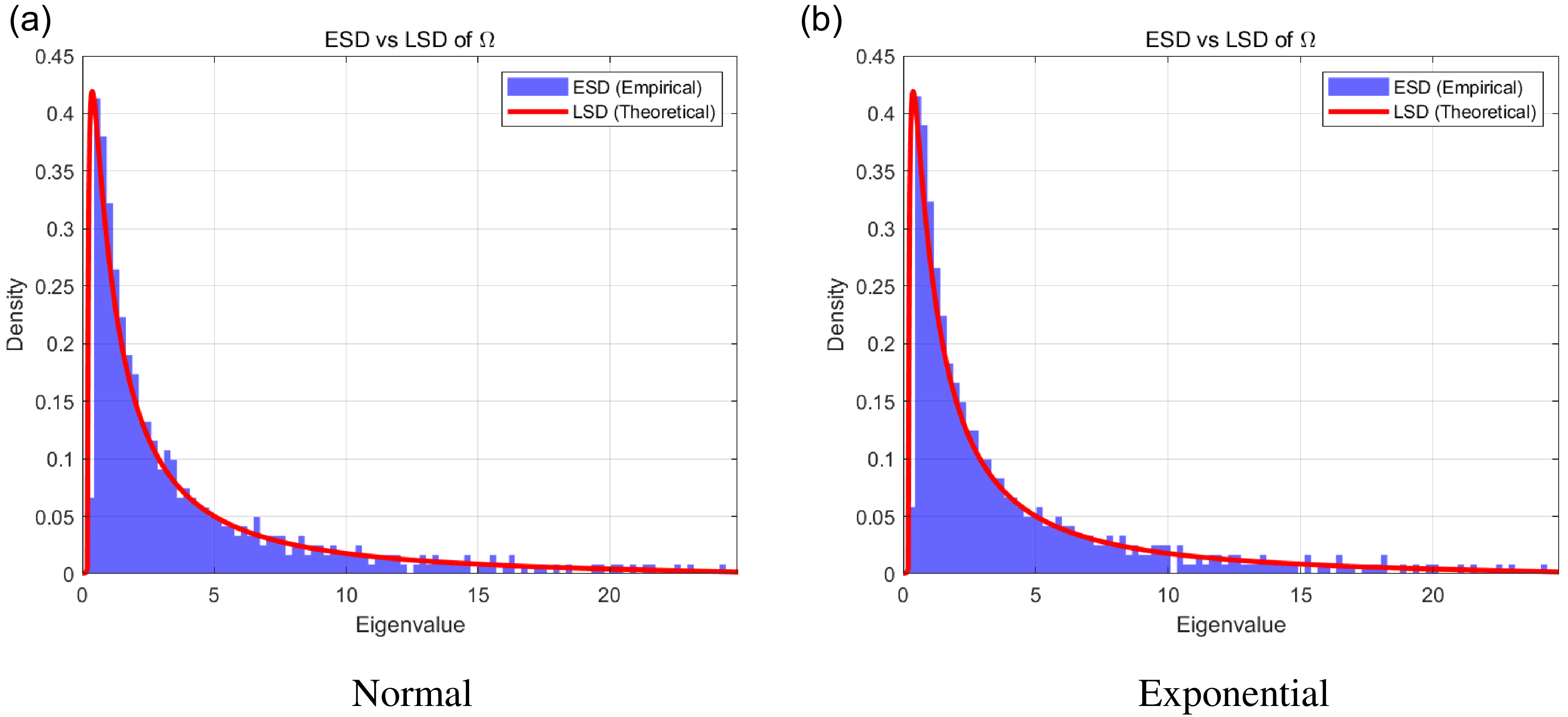
The simulations in this section are conducted to compare the ESD (blue histograms) with the theoretical LSD (red curves) of
 $\boldsymbol{\Omega}$
, providing verification for our Theorem 1. We set the parameters
 $(n, n_1, n_2, p)=(2000, 1000, 1000, 500)$
, which correspond to
 $c_1=c_2=0.5$
. In Figure 1(a), the entries
 $X_{ij}$
are drawn from a standard normal distribution. In Figure 1(b), we set
 $X_{ij}\overset{\mathrm{d}}{=}Y-1$
, where Y follows an exponential distribution with mean 1. The figures demonstrate a close agreement between the ESDs and their theoretical limiting distributions.
 $(n, n_1, n_2, p)=(2000, 1000, 1000, 500)$
.

Figure 1 Long description
Panel A: A histogram compares the empirical spectral distribution (ESD) and the theoretical limiting spectral distribution (LSD) of eigenvalues for a normal dataset. The x-axis represents eigenvalues, and the y-axis represents density. The blue bars represent the empirical data, while the red line represents the theoretical distribution. The empirical data closely follows the theoretical distribution, with a high density of eigenvalues near zero and a rapid decline as eigenvalues increase. Panel B: A histogram compares the empirical spectral distribution (ESD) and the theoretical limiting spectral distribution (LSD) of eigenvalues for an exponential dataset. The x-axis represents eigenvalues, and the y-axis represents density. The blue bars represent the empirical data, while the red line represents the theoretical distribution. Similar to the normal dataset, the empirical data closely follows the theoretical distribution, with a high density of eigenvalues near zero and a rapid decline as eigenvalues increase.
Appendix A. Supporting lemmas
Lemma 1. ([Reference Bai and Silverstein1, Theorem A.43]) Let
 $\mathbf{A}$
and
 $\mathbf{B}$
be two
 $n\times n$
Hermitian matrices. Then
 \begin{align*}\|F^{\mathbf{A}}-F^{\mathbf{B}}\| \leq \frac{1}{n}\mathrm{rank}(\mathbf{A}-\mathbf{B}).\end{align*}
Lemma 2. ([Reference Bai and Silverstein1, Corollary A.41]) Let
 $\mathbf{A}$
and
 $\mathbf{B}$
be two
 $n\times n$
symmetric matrices with their ESDs represented by
 $F^{\mathbf{A}}$
and
 $F^{\mathbf{B}}$
. Then
 $L^3(F^{\mathbf{A}},F^{\mathbf{B}}) \leq \mathrm{tr}((\mathbf{A}-\mathbf{B})^2)/n$
, where
 $L(\cdot, \cdot)$
denotes the Levy distance, i.e.
 \begin{align*} L(F^{\mathbf{A}},F^{\mathbf{B}}) = \inf\big\lbrace \varepsilon \colon F^{\mathbf{A}}(x-\varepsilon,y-\varepsilon) -\varepsilon \leq F^{\mathbf{B}}(x,y) \leq F^{\mathbf{A}}(x + \varepsilon,y + \varepsilon) + \varepsilon\big\rbrace. \end{align*}
Lemma 3. ([Reference Burkholder3, Theorem 21.1]) Let
 ${X_k}$
be a complex martingale difference sequence with respect to the increasing
 $\sigma$
-field
 ${\mathcal{F}_k}$
. Then, for any
 $m \geq 2$
,
 \begin{align*} \mathbb{E}\bigg|\sum X_k\bigg|^m \leq c_m\mathbb{E}\bigg(\sum\mathbb{E}(|X_k|^2|\mathcal{F}_{k-1})\bigg)^{{m}/{2}} + c_m\sum\mathbb{E}|X_k|^m. \end{align*}
Lemma 4. ([Reference Burkholder3, Theorem 20.2]) Under the same conditions as in Lemma 3, for any
 $m \geq 1$
,
 \begin{align*}\mathbb{E}\bigg|\sum X_k\bigg|^m \leq c_m\mathbb{E}\bigg(\sum|X_k|^2\bigg)^{{m}/{2}}.\end{align*}
Lemma 5. ([Reference Li, Bai and Hu5, Lemma 15]) Suppose that, for any
 $\eta>0$
,
 $\sum_{n=1}^{\infty}f(\eta,n) < \infty$
. Then we can select a slowly decreasing sequence of constants
 $\eta_n \to 0$
such that
 $\sum_{n=1}^{\infty}f(\eta_n,n) < \infty$
, where f is a nonnegative function.
Similarly, if
 $f(\eta, n) \to 0$
for any fixed
 $\eta > 0$
, then there exists a decreasing sequence
 $\eta_n \to 0$
such that
 $f (\eta_n, n) \to 0$
.
Declaration
The authors confirm that the AI language model Gemini was utilized for the sole purpose of improving the grammar, spelling, and overall readability of the English in this manuscript. The AI was not used for generating scientific ideas, conducting data analysis, interpreting results, or writing any of the core intellectual content.
Acknowledgements
The authors would like to thank the editor and the reviewer for their careful reading of the manuscript and for the helpful comments that have improved this paper. For correspondence, please contact Yuling Li and Jiang Hu.
Funding information
Jiang Hu was partially supported by NSFC (Grant Nos. 12292980, 12292982, 12571280). Yuling Li was partially supported by the Scientific Research Project of the Education Department of Jilin Province (Grant No. JJKH20250704KJ).
Competing interests
There were no competing interests to declare which arose during the preparation or publication process of this article.
 (n,n1,n2,p)=(2000,1000,1000,500)


