3.1. Mean flow behaviour

Figure 2 permits the definition of a reference separation bubble using the time- and spanwise-averaged flow. We denote time- and spanwise-averaged quantities using a tilde (e.g. $\tilde {U}$). The streamlines (solid black lines) clearly depict the recirculating region within the LSB. The core of the mean recirculating region occurs slightly downstream of the mean bubble height ($\tilde {h}_b = 0.15$ at $\tilde {x} = 3.19$). The mean separation and reattachment points occur at $\tilde {x}_s = 1.76$ and $\tilde {x}_r = 3.80$, respectively, which we can also visually identify in figure 2 with the help of the $\tilde {U} = 0$ isocontour (dashed white line) separating the forward and reverse flow regions. The mean bubble length is therefore $\tilde {L}_b = 2.04$. The mean bubble height, length and streamline pattern agree with those of Spalart & Strelets (Reference Spalart and Strelets2000) (cf. figure 9 in their study). Contours of averaged streamwise velocity show a significant proportion of reversed flow within the LSB relative to the portion of forward flow. In other words, the portion or area of the LSB below the $\tilde {U} = 0$ isocontour is larger than that between the $\tilde {U} = 0$ isocontour and the dividing streamline of the bubble. The curvature of the streamlines near the wall centred at approximately $\tilde {x} = 2.7$ suggests that a small secondary bubble has formed within the larger primary bubble. We note here that the presence of a secondary bubble in this study may very well play a role in the mechanism behind the low-frequency unsteadiness. Cherubini, Robinet & De Palma (Reference Cherubini, Robinet and De Palma2010) demonstrate that such a topological change in the base flow of a 2-D LSB can produce a low-frequency unsteadiness as a result of the superposition of convective non-normal modes. However, Pauley et al. (Reference Pauley, Moin and Reynolds1990) observe a quasi-periodic phenomenon in their 2-D LSB simulations where the secondary bubble grows and pinches off a portion of the larger bubble which is then advected downstream. We do not observe such a pinch-off phenomenon in our 3-D simulations. Nevertheless, as suggested by the work of Tafti & Vanka (Reference Tafti and Vanka1991b), low-frequency unsteadiness appears to require a 3-D study and it is likely not the case that a 2-D analysis can adequately capture the dynamics of the phenomenon.

Figure 2.

Time- and spanwise-averaged streamwise velocity $\tilde {U}$ of the laminar separation bubble. Streamlines are depicted using solid black lines and the $\tilde {U} = 0$ isocontour using a dashed white line.

In figure 3, we illustrate several critical curves to further characterize the time- and spanwise-averaged separation bubble. The dividing streamline (solid black line) is computed as the locus of points where the integral of the streamwise velocity is zero starting from the wall (i.e. $\int _0^{y_{d}}\tilde {U}(x,y)\,\mathrm{d}y = 0$). The dividing streamline is skewed towards the aft portion of the bubble, in other words, the streamwise length from separation to peak ($\Delta \tilde {x} = 1.43$) is longer than that from peak to reattachment ($\Delta \tilde {x} = 0.61$). The skewed shape of the bubble is expected given the overall direction of the flow, causing a general streamwise elongation of the bubble, and the rapid transition to turbulence in the aft portion of the bubble, prompting rapid reattachment. Given the enlarged wall-normal scale in figure 3, we can observe the dividing streamline of the secondary bubble. The mean separation and reattachment points of the secondary bubble are located respectively at $\tilde {x}_{s_2} = 3.01$ and $\tilde {x}_{r_2} = 2.85$. Bear in mind that $\tilde {x}_{r_2} < \tilde {x}_{s_2}$ for the secondary bubble as it separates downstream and reattaches upstream due to the reverse flow induced by the primary bubble. The isocontour $\tilde {U} = 0$ (dashed red line) in figure 3 demonstrates more clearly the significant portion of reverse flow present in the separation bubble relative to the portion of forward flow contained between the dividing streamline and the $\tilde {U} = 0$ isocontour. The locus of points marking the locations of maximum reverse flow (dash-dotted blue line) demonstrates the asymmetry within the region of reversed flow (i.e. below $\tilde {U} = 0$). The maximum reversed flow $\tilde {u}_{rev} = 16.8\,\%$ occurs at $\tilde {x} = 3.32$ and $\tilde {y} = 0.0135$. The present LSB therefore possesses a maximum reverse flow within the range of absolute instability proposed by Alam & Sandham (Reference Alam and Sandham2000) and Rist & Maucher (Reference Rist and Maucher2002). The locations of peak reversed flow occur further away from the wall in the fore portion of the bubble than in the aft portion, this again being due to transition to turbulence in the aft portion. The location of peak reversed flow occurs furthest from the wall between the peak height and reattachment of the secondary bubble $(\tilde {x} = 2.90)$. The locus of the first inflection points of the streamwise velocity from the wall (solid green line) highlights the importance of the secondary bubble in the observed behaviour of the primary bubble. The inflection curve begins at $\tilde {x}_{i} = 2.60$. Avanci et al. (Reference Avanci, Rodríguez and Alves2019) propose that absolutely unstable Kelvin–Helmholtz waves for an LSB requires that the inflection point falls below the dividing streamline. For the present LSB, the formation of the secondary bubble is accompanied by a surrounding ‘bubble’ of inflection of the streamwise velocity profile lying within the dividing streamline of the larger primary bubble. The proposed condition of Avanci et al. (Reference Avanci, Rodríguez and Alves2019) is therefore satisfied, on average, in the present study. We therefore expect to observe upstream propagation of disturbances and unstable behaviour in the vicinity of $\tilde {x}_{i} = 2.60$. Cherubini et al. (Reference Cherubini, Robinet and De Palma2010) demonstrate that disturbances introduced in the first half of a (2-D) LSB are amplified to nearly the same extent as disturbances introduced entirely upstream of separation. If the low-frequency unsteadiness is a phenomenon that is excited by free stream disturbances, an absolute instability within the LSB combined with the observations of Cherubini et al. (Reference Cherubini, Robinet and De Palma2010) suggest that free stream disturbances may not be a necessary criterion for the onset of low-frequency unsteadiness in LSBs when a secondary bubble is formed.

Figure 3.

Time- and spanwise-averaged dividing streamlines (solid black lines), $\tilde {U} = 0$ isocontour (dashed red line), maximum reversed flow (dash-dotted blue line) and streamwise velocity inflection (solid green line).

Figure 4 shows the evolution of the wall pressure and friction coefficients in the streamwise direction computed from the time- and spanwise-averaged flow field. To compare with the results of Spalart & Strelets (Reference Spalart and Strelets2000) whose separation point occurs at $\tilde {x}_s = 2.25$, we simply shift their data upstream such that their separation point coincides with that of the present study ($\tilde {x}_s = 1.76$). This shift is due to the treatment of their inflow and outflow with the fringe method that ends at $x \simeq 0.5$ from the domain virtual origin, thus imposing a ‘useful region’ smaller than the full computational domain. The wall pressure coefficient, shown in figure 4(a), is defined by $\tilde {C}_p = (\tilde {P} - P_{\infty })/(\frac {1}{2}\rho U_{\infty }^2)$, where $P_{\infty }$ is the pressure at the inlet section and $\tilde {P}$ is the time- and spanwise-averaged wall pressure. The wall pressure coefficient agrees very well with the DNS of Spalart & Strelets (Reference Spalart and Strelets2000). The presence of the suction profile (peak at $x = 2.50$) causes an APG to begin to develop upstream of separation, resulting in a gradual thickening of the boundary layer (cf. figure 5) and increase in $\tilde {C}_p$. A pressure plateau then arises from the displacement of the boundary layer accompanying the separated flow in the vicinity of peak suction. This is followed by a steep increase in pressure prior to and past reattachment $(\tilde {x}_r = 3.80)$ due to the transition to turbulence. The wall pressure coefficient eventually reaches a constant value towards the end of the flow domain ($x = 8$), which is different from the inlet value due to the portion of flow that is extracted and not reinjected.

Figure 4.

(a) Time- and spanwise-averaged wall pressure coefficient $\tilde {C}_p$. (b) Time- and spanwise-averaged skin friction coefficient $\tilde {C}_f$ (solid black line) and fluctuating skin friction coefficient $\tilde {C}'_f$ (dashed blue line). The results of Spalart & Strelets (Reference Spalart and Strelets2000) are represented by the circular markers.

Figure 5.

(a) Time- and spanwise-averaged displacement thickness $\tilde {\delta }^*$ and (b) momentum thickness $\tilde {\theta }$. Solid lines denote the results of the present study and the circular markers those of Spalart & Strelets (Reference Spalart and Strelets2000).

We present the skin friction coefficient $\tilde {C}_f = \tilde {\tau }_w /(\frac {1}{2}\rho U_{\infty }^2)$ (solid black line) and its fluctuating counterpart $\tilde {C}'_f$ (dashed blue line) with streamwise position in figure 4(b), where $\tilde {\tau }_w$ is the time- and spanwise-averaged wall shear stress. The locations of the mean separation and reattachment points are defined as the points where $\tilde {C}_f$ is zero and where $\tilde {C}'_f$ has attained a local maximum. It is interesting to observe that $\tilde {C}'_f$ peaks at mean separation, implying that the separation surface does exhibit some small excursions in the streamwise direction. Past mean separation $(\tilde {x}_s = 1.76)$, the skin friction coefficient $\tilde {C}_f$ attains a local minimum followed by a weak increase in amplitude (positive slope). The skin friction does cross the abscissa and changes sign in the range $2.80 < \tilde {x} < 2.94$, which agrees with the location of the secondary bubble described earlier using its dividing streamline. We observe that the results of Spalart & Strelets (Reference Spalart and Strelets2000) indicate a minimum $\tilde {C}_f$ slightly larger in magnitude than that of the present study. Furthermore, the skin friction coefficient of Spalart & Strelets (Reference Spalart and Strelets2000) shows slight variations particularly past reattachment whereas our results show a smooth decay. The observed differences in the skin friction coefficient (as well as in the displacement and momentum thicknesses in figure 5) with those of Spalart & Strelets (Reference Spalart and Strelets2000) are likely due to the long time interval used for averaging in our study, namely, $5\,600$ snapshots spanning a total non-dimensional time of 1400 ($\Delta t = 0.25$). No significant differences are observed using a longer averaging time.

Following Spalart & Strelets (Reference Spalart and Strelets2000), we also present the time- and spanwise-averaged displacement $\tilde {\delta }^*$ and momentum $\tilde {\theta }$ thicknesses in figure 5 and compare with their results for validation. Following their approach, the boundary layer thicknesses are computed based on the pseudo-free stream velocity defined as the integral of the spanwise vorticity along the wall-normal direction $\bar {U}(x,y)= -\int _{0}^{y}\omega _z (x,y')\,\mathrm {d}y'$. The displacement thickness $\tilde {\delta }^*$ (cf. figure 5a) increases slowly up to separation due to the upstream influence of the imposed APG. The displacement thickness then increases abruptly as the boundary layer separates from the wall and peaks near the maximum bubble height $(\tilde {x} = 3.19)$. Approaching reattachment, the bubble height is diminished and therefore accompanied by a decrease in displacement thickness which continues past reattachment until attaining a weakly increasing plateau in the TBL. The momentum thickness $\tilde {\theta }$ (cf. figure 5b), however, increases slowly up to the location of the secondary bubble and the onset of spanwise roller formation where a slight decrease is observed. This location occurs slightly before the maximum bubble height where breakdown of spanwise rollers appears to begin. The breakdown of spanwise rollers results in an important loss of momentum in the boundary layer and consequently a rapid increase in momentum thickness until also attaining a weakly increasing plateau in the developing TBL. Again, the observed differences in the boundary layer thicknesses with those of Spalart & Strelets (Reference Spalart and Strelets2000), particularly past reattachment, are likely due to averaging over a longer time interval in our study.

3.2. Instantaneous flow behaviour

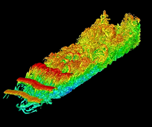
In figure 6, we visualize unsteady vortical structures using isosurfaces of $\lambda _2$ (Jeong & Hussain Reference Jeong and Hussain1995) at a selected time instant ($t = 1146.5$), where the colour scale represents the local instantaneous streamwise velocity. Shedding of coherent spanwise rollers occurs near $x = 2.7$, which is situated close to the start of the mean inflection curve of the secondary bubble $(\tilde {x}_i = 2.60)$. The vortex shedding occurs at a frequency (equivalent to a Strouhal number, based on $U_\infty$ and $h$) of $St = 1.56$ based on the pre-multiplied power spectral density (PSD) of the velocity fluctuations $u'$ and $v'$ close to the mean position of maximum bubble height $(x,y,z) = (3,0.15,0)$; cf. figure 7. The rollers are shed from the shear layer with what appears to be immediate spanwise undulations having a spanwise wavelength of approximately twice that of the streamwise wavelength, as also observed by Michelis, Yarusevych & Kotsonis (Reference Michelis, Yarusevych and Kotsonis2018). Such spanwise undulations can arise as a result of unstable oblique disturbances present upstream of shear layer rollup (Michelis et al. Reference Michelis, Yarusevych and Kotsonis2018). Oblique disturbances may be present entirely upstream of separation as a result of upstream propagation of numerical error (Spalart & Strelets Reference Spalart and Strelets2000). Nevertheless, we also observe near-wall vortical structures in figure 6 as early as $x = 2.6$, in particular, the lifting-up and reversal of a $\varLambda$-like vortex initially propagating upstream due to the reversed flow near the wall. The formation of the near-wall structures occurs necessarily at the expense of streamwise momentum, retarding the flow in its vicinity. This may be a cause of the observed undulation in the spanwise rollers. However, at this stage, we may also conjecture the reverse and suggest that the spanwise undulation of the rollers, due to some underlying instability, induces a secondary or tertiary instability near the wall. Following the formation of the spanwise rollers, their breakdown begins near the mean location of maximum bubble height $(\tilde {x} = 3.19)$, as also observed by Simoni et al. (Reference Simoni, Ubaldi and Zunino2014). Breakdown of the rollers is a result of several factors including secondary instabilities of and between the vortex cores (Marxen, Lang & Rist Reference Marxen, Lang and Rist2013) and, as we observe, their interaction with the structures forming at the wall. The transition to turbulence occurs abruptly prior to reattachment, within only 2–3 streamwise wavelengths.

Figure 6.

Instantaneous isosurfaces of $\lambda _2=-5$, coloured by streamwise velocity, in perspective and top views at $t = 1146.5$.

Figure 7.

Pre-multiplied power spectral density of instantaneous velocity at $x = 3$, $y = 0.15$ and $z = 0$ for (a) $u'$ and (b) $v'$.

We further dissect the 3-D behaviour in figure 8 using contours of vorticity magnitude at the same instant within the wall plane, a spanwise boundary and within the $x = 2.6$, $3.0$, $3.9$ and $4.5$ planes. In the wall plane, vorticity magnitude appears as far upstream as $x \sim 2.4$, demonstrating that the small-scale near-wall structures observed in figure 6 emerge and develop prior to shear layer rollup and even before the mean streamwise velocity inflection caused by the secondary bubble. The transverse planes at $x = 2.6$ and $3.0$ show a considerable increase in vorticity magnitude generated within the bubble (i.e. below the clearly visible shear layer). By $x = 3.9$, just past reattachment, the vorticity magnitude already suggests a rather turbulent flow and we begin to see the ‘peaks’ and ‘valleys’ observed by Spalart & Strelets (Reference Spalart and Strelets2000). Packets of vorticity are being ejected away from the wall (the ‘peaks’), while other portions are drawn towards the wall (the ‘valleys’). These peaks and valleys persist downstream and possess the same spanwise wavelength as the undulations we observe in the spanwise rollers. At $x = 4.5$, the peaks and valleys of vorticity are more apparent and appear in reverse order from those at $x = 3.9$. From the vorticity plotted in the spanwise boundary, we observe that the structures at $x = 4.5$ are part of a disconnected packet of vorticity from those at $x = 3.9$.

Figure 8.

Contours of vorticity at the bottom wall, the $z = -0.3$ plane and at selected $yz$ planes at $x = 2.6$, $3.0$, $3.9$ and $4.5$.

In figure 9, we show isosurfaces of $u' = -0.12$ (blue) and $u' = 0.12$ (red) at the same time instant of figures 6 and 8. We observe that the ‘peak’ observed in the $x = 4.5$ plane coincides with a region of negative $u'$ and the ‘valley’ with a region of positive $u'$. The portions of fluid ejected from the wall are therefore deficient in streamwise momentum relative to the mean. The regions of positive and negative $u'$ occur on a rather large scale displaying a spanwise wavelength of the order of the domain width ($\lambda _z \sim 0.6$) and an elongation in the streamwise direction ($\lambda _x > 1$), similar to the large-scale ejection and sweep motions observed in TBLs in the form of streaks (Adrian Reference Adrian2007). Spalart & Strelets (Reference Spalart and Strelets2000) identify streaks further downstream, yet in figure 9, we can observe the streaks extending well within the LSB ($\tilde {x}_r = 3.80$). Hosseinverdi & Fasel (Reference Hosseinverdi and Fasel2019) recently demonstrated the importance of the occurrence and amplification of streaks in LSBs as they play an important role in the transition process for moderate ($0.5$ to $1$ %) to high ($2$ to $3$ %) free stream turbulence intensity. In our study, free stream turbulence is due only to numerical error and is $O(10^{-5})$ to $O(10^{-4})$. The Klebanoff (or K) mode is therefore not expected to be a dominant mechanism in the transition to turbulence of the present LSB in view of the work of Hosseinverdi & Fasel (Reference Hosseinverdi and Fasel2019).

Figure 9.

Instantaneous isosurfaces of $| u'| = 0.12$, represented by blue (negative $u'$) and red (positive $u'$).

Figure 10 shows the probability density function with respect to the variables $u'$ and $v'$ within the 3-D domain at two time instants, one at which the LSB appears smaller than the mean ($t = 1370.75$) and the other at which it appears larger than the mean ($t = 1146.5$). When the LSB appears smaller ($t = 1370.75$), the probability density function shows predominant fluctuations in the fourth quadrant $(Q4)$, namely, fluctuations having positive $u'$ and negative $v'$. When the LSB appears larger ($t = 1146.5$), the probability density function shows predominant fluctuations in the second quadrant $(Q2)$, namely, fluctuations having negative $u'$ and positive $v'$. A predominance of sweep-like structures $(Q4)$ is therefore linked to shrinkage of the bubble relative to the mean and of ejection-like structures $(Q2)$ to growth of the bubble. While we certainly do not have a fully developed TBL, it is interesting to observe that the quadrant analysis is converging towards what is expected in TBLs (Adrian Reference Adrian2007).

Figure 10.

Normalized probability density function of $u'$ and $v'$ within the 3-D domain (a) when the LSB is smaller than the mean size ($t = 1370.75$) and (b) when the LSB is larger than the mean size ($t = 1146.5$). The colour scale represents the probability from white (zero) to black (one).

Marxen & Rist (Reference Marxen and Rist2010) demonstrate the role of so-called mean flow deformation in LSBs, where the amplification of disturbances causes a reduction in the mean size of the bubble. From the perspective offered by the quadrant analysis, the addition of the mean flow will ‘shift’ events from the second quadrant of the $(u', v')$ plane into the first quadrant of the $(u, v)$ plane, while events in the fourth quadrant will largely remain within the fourth quadrant. The presence or development of disturbances in the present LSB therefore bias the flow towards the fourth quadrant in the $(u, v)$ plane (sweep-like motions) such that a simple ensemble mean will forcibly produce events in the second quadrant, whether these events are physical or not. In other words, in the case of an LSB, it may be more beneficial to our understanding if we adopt the perspective of a base flow with perturbations rather than the classical turbulence approach of an ensemble mean with fluctuations. The reduction in the size of the bubble associated with a receding reattaching surface can then be seen as the passage of a group of sweep-like perturbations with varying spanwise intensity emerging either from within the LSB or from free stream turbulence upstream of the LSB. Conversely, the growth of the bubble associated with the downstream excursion of the reattaching surface corresponds to a return to an ‘unforced’ state when these perturbations pass. This perspective is not only consistent with the observed mean flow deformation in LSBs (Marxen & Rist Reference Marxen and Rist2010), but provides a link between the ‘flapping’ dynamics and the observation of spanwise alternating patterns of streak-like motions in the fluctuating flow field.

3.3. Low-frequency unsteadiness

In figure 11, we show the variation of the spanwise-averaged wall pressure with time in the aft portion of the LSB. The location of the mean reattachment point is marked by a dashed white line. The spectral content of the spanwise-averaged wall pressure is clearly rich in frequencies, similar to experimental (Mohammed-Taifour & Weiss Reference Mohammed-Taifour and Weiss2016) and numerical (Wu, Meneveau & Mittal Reference Wu, Meneveau and Mittal2020) observations from TSBs. We observe several intermittent events acting over many different time scales, from frequencies in the range of the vortex shedding $(St \sim 1)$ to very low frequencies $(St \sim 0.001)$. Excursions on a time scale of $t \sim 100$ are also apparent and, upon closer inspection, we observe excursions on a time scale of $t \sim 10$. These lower frequency excursions of the wall pressure occur most clearly prior to reattachment (i.e. between $x \sim 3.4$ and $3.7$). The continuous wavelet transform of the wall-pressure fluctuations at $x = 3.0$ (figure 12a) shows the dominance of the high-frequency regime at $St \sim 1.5$, where vortex shedding occurs. Low-frequency signatures are also observed. Closer to reattachment, at $x = 3.47$ (figure 12b), the low-frequency regime with $St \sim 0.1$ is predominant. Signatures at even lower frequencies are also clearly observed, as low as $St \sim 0.01$. However, such events are characterized by a strong intermittency which may not be clearly detected by more classical spectral analysis.

Figure 11.

Evolution of spanwise-averaged wall pressure with time.

Figure 12.

Wavelet analysis of spanwise-averaged wall pressure at (a) $x = 3.0$ and (b) $x = 3.47$.

To further examine the frequency content of the wall pressure, figure 13 shows the power spectra taken at various streamwise locations. Far upstream $(x \sim 0)$, no dominant frequencies appear. As we approach mean separation $(\tilde {x}_s = 1.76)$, we observe an overall amplification of low frequencies and, in particular, the emergence of a peak centred at $St \sim 0.08$ which continues to grow up to mean reattachment $(\tilde {x}_r = 3.80)$. This amplification of low-amplitude, low-frequency spectral content suggests that low-frequency upstream disturbances, however small, exist ahead of separation and are selectively amplified by the deceleration imposed by the APG and later by the separation bubble itself (Cherubini et al. Reference Cherubini, Robinet and De Palma2010). The amplification is significant in the case of LSBs, with Rist & Maucher (Reference Rist and Maucher2002) suggesting that upstream disturbances even of order $10^{-4}$ can be considered high. In figure 13, the low frequency centred at $St \sim 0.08$ persists long past mean reattachment, including some of its harmonics. The persistence of the low frequency downstream of reattachment suggests that it is associated with the advection of spatiotemporally coherent structures downstream. Normalizing the dominant low-frequency unsteadiness with the mean length of the separation bubble yields $St_{b} = 0.163$ which falls within the range 0.08–0.2 of flapping frequencies previously reported by Hudy et al. (Reference Hudy, Naguib and Humphreys2003) in geometry-induced separation bubbles. Michelis, Yarusevych & Kotsonis (Reference Michelis, Yarusevych and Kotsonis2017) and Jaroslawski et al. (Reference Jaroslawski, Forte, Vermeersch, Moschetta and Gowree2023) used the displacement thickness $\delta ^*$ at the separation point to normalize frequencies, and both studies found that the low-frequency Strouhal number is below $St_{\delta ^*}=0.005$, although without clearly identifying an emerging spectral peak, but this is consistent with our low frequency of $St_{\delta ^*}=0.002$. Within the LSB, from $x \sim 2.60$, a higher frequency peak centred at $St \sim 1.52$ begins to emerge and amplify which corresponds to the vortex shedding. Normalized with the momentum thickness and the local free stream velocity at separation, the Strouhal number for vortex-shedding is $St_\theta = 0.0067$, which is slightly lower than the references presented by Rodríguez et al. (Reference Rodríguez, Gennaro and Souza2021) (see their table 1), but is very close to the value of 0.0068 reported by Pauley et al. (Reference Pauley, Moin and Reynolds1990) and of 0.0062 obtained by Jaroslawski et al. (Reference Jaroslawski, Forte, Vermeersch, Moschetta and Gowree2023). However, care must be taken concerning such comparisons. In the case of Jaroslawski et al. (Reference Jaroslawski, Forte, Vermeersch, Moschetta and Gowree2023), separation is studied on an aerofoil, where reference quantities used for scaling might not have a clear definition. More importantly, Pauley et al. (Reference Pauley, Moin and Reynolds1990) conducted a 2-D simulation, while in the 3-D case performed by the same first author (Pauley Reference Pauley1994), the Strouhal number is approximately twice that of the 2-D case. In the present study, imposing non-natural periodic conditions in the spanwise direction should better match the 2-D case (cf. Alizard, Cherubini & Robinet (Reference Alizard, Cherubini and Robinet2009), who obtained the same Strouhal numbers by investigating the linear convective instability mechanism), as in experiments, these conditions cannot be imposed. With $x = 2.60$ corresponding to the earliest location of inflection in the streamwise velocity profile, by the criterion of Avanci et al. (Reference Avanci, Rodríguez and Alves2019), the high-frequency shedding may be triggered by an absolute instability of the bubble. From mean reattachment $(\tilde {x}_r = 3.80)$ onwards, this high-frequency peak decays rapidly unlike the low-frequency peak. As observed in the instantaneous flow fields in figures 6 and 8, the spanwise rollers rapidly breakdown even prior to reattachment.

Figure 13.

Power spectral density of wall-pressure fluctuations.

In figure 14(a), we isolate the amplification of the low $(St \sim 0.08)$ and high $(St \sim 1.52)$ frequencies observed in the power spectra of the spanwise-averaged wall pressure with streamwise location. The low frequency shows exponential growth ahead of separation likely due to the effects of the APG from the imposed suction extending upstream. At separation, the amplification of the low frequency slows as the higher frequency begins to grow exponentially. The high frequency peaks at $x \sim 3.2$, at the maximum bubble height, and subsequently decays coinciding with the undulation and breakdown of the shed vortices in figure 6. The low frequency exhibits a second stage of rapid growth coinciding with the initial location of velocity profile inflection caused by the presence of the secondary bubble $(x \sim 2.6)$. This is followed by a third stage coinciding with the peak of the high-frequency amplification. The third stage of growth of the low frequency occurs regardless of the breakdown of the shed vortices. The low frequency attains its peak at $x \sim 3.5$, after which it weakly decays until remaining rather constant and yet significantly more dominant than the shedding frequency.

Figure 14.

(a) Power spectral density of the two selected dominant frequencies of pressure at the wall. (b) Maximum root-mean-square of velocity fluctuations within the boundary layer.

The amplification patterns of the high- and low-frequency signatures respectively resemble those of the spectral disturbance kinetic energies of the 2-D Kelvin–Helmholtz modes (fundamental frequency) and the 3-D Klebanoff modes (low frequency) observed by Hosseinverdi & Fasel (Reference Hosseinverdi and Fasel2019). They show that the higher the level of free stream turbulence, the earlier and more significant the amplification of the low-frequency Klebanoff streaks. While we cannot eliminate upstream disturbances caused by numerical propagation in our study, we maintain that the velocity fluctuations upstream are initially fairly weak $O(10^{-5})$; cf. figure 14(b). However, prior to separation, all fluctuations have exhibited significant amplification, as suggested by Rist & Maucher (Reference Rist and Maucher2002) and Cherubini et al. (Reference Cherubini, Robinet and De Palma2010). By comparing figure 14(a) with the results in figure 18 of Hosseinverdi & Fasel (Reference Hosseinverdi and Fasel2019), we observe that the low frequency attains its peak amplification later than the high frequency in the present LSB, whereas the reverse is true in the study by Hosseinverdi & Fasel (Reference Hosseinverdi and Fasel2019). Given that we do not explicitly introduce such disturbances in our study, the delay in the low-frequency peak indicates that other factors (e.g. the secondary bubble) can still result in a dominant low-frequency unsteadiness in the case of low free stream turbulence. Furthermore, we infer from figures 6, 8 and 9 that the disturbances generated within the LSB itself may be a sufficient trigger to low-frequency unsteadiness in the absence of free stream turbulence altogether. In view of the results of Spalart & Strelets (Reference Spalart and Strelets2000), the velocity fluctuations in the inlet region are one order of magnitude higher than those observed in figure 14(b). This discrepancy can be attributed to differences in the initial conditions, as their study used 3-D random perturbations, whereas our present study does not include any perturbations. Moreover, they found that velocity fluctuations ($u'$ and $w'$) within the boundary layer exist and grow upstream of separation until attaining maxima near reattachment, after which the largest fluctuations roughly stabilize or weakly decay. We show this behaviour in figure 14(b) for all three velocity fluctuations. The three velocity fluctuations follow a similar amplification behaviour as the low frequency up to their peak at $x \sim 3.5$, with the growth of $u'$ being the most significant. This suggests that the low frequency is correlated with a significant source of $u'$ in the flow. The growth of $w'$ is very steep at separation, whereas that of $u'$ is slowed and $v'$ slowed to a lesser extent. While this indeed demonstrates that the 3-D characteristics are amplified soon after separation, it is also suggestive of a realignment of spanwise vorticity into streamwise or wall-normal vorticity, both of which can produce regions of low and high streamwise momentum.

In TSBs, the low frequency is attributed to a so-called breathing motion, where the bubble grows and shrinks in size. In LSBs, flapping refers to the wavering of the shear layer and therefore to excursions of the reattachment surface upstream and downstream. In a sense, flapping of an LSB has the low-frequency signature of a ‘half-breathing’ of a TSB. To analyse the unsteadiness in the shape and size of the LSB, we therefore follow Pearson, Goulart & Ganapathisubramani (Reference Pearson, Goulart and Ganapathisubramani2013) and Mohammed-Taifour & Weiss (Reference Mohammed-Taifour and Weiss2016), and compute conditional averages based on the reverse flow area. As a measure of reverse flow area, we simply compute the fraction of nodes possessing a negative streamwise velocity. Figure 15(a) shows the temporal evolution of the fraction of reverse flow computed within the midspan plane (blue) and over the whole 3-D domain (black). The mean fraction of reverse flow is approximately $0.06$ for both the 2-D and 3-D computations. The temporal oscillations of the fraction of reverse flow reveal a quasi-periodic expansion (larger fraction) and contraction (smaller fraction) of the bubble. We show the power spectrum of the fraction of reverse flow in figure 15(b). We observe a dominant low-frequency peak at $St = 0.06$. This frequency is close to that reported earlier in figure 13 $(St = 0.08)$, the difference largely arising from the pollution of the fraction of reverse flow signal by considering the whole domain, whereas the pressure is averaged only at the wall.

Figure 15.

(a) Fraction of reverse flow area (fRFA) over the whole 3-D domain (solid black line) and within the midspan plane (dashed blue line). (b) Power spectral density of the fraction of reverse flow area computed from the 3-D domain.

To capture the flapping motion of the LSB and therefore its expansion and contraction, we now perform conditional averages based on the fraction of reverse flow. Figure 16 shows the dividing streamlines of the LSB in its minimum, mean and maximum states within the midspan plane using conditional averages. The minimum and maximum bubble sizes are based on those instants with a fraction of reverse flow lying respectively below and above $1.5$ standard deviations from the mean, which essentially captures the minima and maxima at the low frequency. While there is a noticeable streamwise excursion of the reattaching surface of length $\Delta x_r = 0.4$, there is only a slight variation at separation (of the order of $2\Delta x$), as confirmed by the fluctuating skin friction coefficient $\tilde {C}'_f$ in figure 4(b). The expansion and contraction of the bubble in the wall-normal direction is also clearly observed, corresponding to the so-called ‘flapping’ or ‘wavering’ motion of the shear layer.

Figure 16.

Conditionally averaged dividing streamlines using the fraction of reverse flow area. The minimum (dash-dotted green line), mean (solid white line) and maximum (dashed black line) states are shown. Contours represent the time- and spanwise-averaged streamwise velocity for reference.

3.4. Modal decomposition

Up to this point, we have shown that the present LSB may be subject to an absolute instability, as proposed by Avanci et al. (Reference Avanci, Rodríguez and Alves2019), arising from the formation of a secondary bubble within the larger primary LSB. This instability is supported by the presence of an inflection of the streamwise velocity falling below the dividing streamline of the primary LSB within the range $2.60 < \tilde {x} < 3.14$ as well as the onset of spanwise roller formation near $x = 2.60$, namely the start of the inflection curve. Accompanying the supposed instability is the propagation of near-wall disturbances upstream. Indeed, we do also observe spots of near-wall vortical structures forming from $x \geqslant 2.40$ in the instantaneous flow field. The consequence of these structures is to retard the flow in the streamwise direction, causing a rapid spanwise undulation in the rollers of wavelength ${\sim }6$ times that of the diameter of the rollers, or approximately twice the streamwise wavelength of the rollers. Despite spanwise roller breakdown beginning at maximum bubble height $(\tilde {x} \sim 3.19)$, the peaks and valleys observed further downstream in the instantaneous flow fields appear to preserve this spanwise wavelength (up to at least $x \sim 8$).

We observe a particular low-frequency signature with $St \sim 0.08$. By comparison with the fraction of reverse flow, we are able to show that expansion (more reverse flow) and contraction (less reverse flow) occur for the LSB at a similar frequency, similar to the breathing motion observed in the context of TSBs. In the case of an LSB, this motion occurs largely on the reattachment side where wavering of the shear layer causes the reattachment surface to migrate upstream and downstream. Furthermore, the low frequency was observed to exhibit three stages in its amplification: (1) early amplification by the APG; (2) slowed growth coinciding with the excitation of spanwise rollers; (3) renewed amplification coinciding with the formation and rapid breakdown of the spanwise rollers. The low frequency subsequently decays to a plateau further downstream. The growth of all three velocity fluctuations within the boundary layer follows a similar tendency, the peak instead occurring at the location of roller breakdown. The low frequency is therefore strongly linked to the amplification of velocity fluctuations and their persistence downstream.

The third stage of amplification of the low frequency coincides with the formation of the near-wall structures $(\tilde {x} = 2.60)$ observed in figures 6 and 8. Given that the velocity fluctuations within the boundary layer are only amplified up to spanwise roller breakdown, this suggests that they too are associated with the dynamics caused by the near-wall structures, namely the local deceleration of the flow, the undulation of the spanwise rollers and the persistence of this wavelength downstream in the form of large streamwise packets of vortical structures which cause the peaks and valleys observed in the instantaneous flow field. As a consequence, it appears that the low-frequency behaviour is linked to the effects and propagation of flow that is deficient in streamwise momentum (more negative $u'$) and flow that is not (more positive $u'$), bearing some resemblance to the low- and high-speed streaks in TBLs. Proper elucidation of these structures and whether they truly are tied to the low-frequency unsteadiness requires an extraction and analysis of the coherent structures of the flow. In what follows, we use modal decomposition methods to elucidate these structures and analy-e their behaviour in the context of the low frequency unsteadiness.

3.4.1. Proper orthogonal decomposition

Proper orthogonal decomposition (POD) is a commonly used technique to decompose a turbulent flow into spatially coherent modes ranked by their turbulent kinetic energy. In this section, we apply space-only POD using the method of snapshots (Sirovich Reference Sirovich1987) rather than spectral POD which is concerned with spatiotemporal coherence (Towne, Schmidt & Colonius Reference Towne, Schmidt and Colonius2018).

Briefly, we define the snapshot matrix $\boldsymbol {X}$ as the collection of all snapshots (i.e. discrete time instants $k$) of the fluctuating velocity field as follows:

(3.1)\begin{equation} \boldsymbol{X} = \begin{bmatrix} \mid & & \mid & & \mid\\ \boldsymbol{x}_1 & \cdots & \boldsymbol{x}_k & \cdots & \boldsymbol{x}_n\\ \mid & & \mid & & \mid \end{bmatrix} \quad\text{where}\ \boldsymbol{x}_k = \begin{bmatrix} \boldsymbol{u}'_k\\ \boldsymbol{v}'_k\\ \boldsymbol{w}'_k \end{bmatrix}. \end{equation}

In space-only POD, the flow is represented by a linear combination of spatially orthogonal modes, each with their own time dynamics, which can be expressed succinctly as

(3.2)\begin{equation} \boldsymbol{X} = \boldsymbol{\varPhi}\boldsymbol{A}, \end{equation}

where the columns $\boldsymbol {\phi }_k$ of $\boldsymbol {\varPhi }$ denote the proper orthogonal modes and the rows $\boldsymbol {a}_k$ of $\boldsymbol {A}$ denote their respective time dynamics. The proper orthogonal modes and their time dynamics are computed from

(3.3a,b)\begin{equation} \boldsymbol{\varPhi} = \boldsymbol{X}\tilde{\boldsymbol{\varPhi}}\boldsymbol{\varLambda}^{{-}1/2} \quad \text{and} \quad \boldsymbol{A} = \boldsymbol{\varPhi}^\mathrm{T}\boldsymbol{X}, \end{equation}

where $\boldsymbol {\varLambda }$ and $\tilde {\boldsymbol {\varPhi }}$ represent the eigenvalues and eigenvectors, sorted in decreasing order of $\boldsymbol {\lambda }_k$, of the following eigenvalue problem:

(3.4)\begin{equation} \boldsymbol{C}\tilde{\boldsymbol{\varPhi}} = \tilde{\boldsymbol{\varPhi}}\boldsymbol{\varLambda} \end{equation}

with correlation matrix $\boldsymbol {C} = \boldsymbol {X}^\mathrm {T}\boldsymbol {X}$.

We perform space-only POD using $3000$ snapshots of the 3-D flow field extracted in increments of $\Delta t = 0.05$. The total time considered is therefore $150$, which we found to be sufficient; no significant differences were observed using as few as $1000$ snapshots. The spatial domain spans the entire spanwise width $z \in [0,0.6]$ and is limited to $x \in [1.5,4.7]$ in the streamwise direction and $y \in [0,0.5]$ in the wall-normal direction, encompassing key features of the separated and reattached flow. Given the large volume of data, we compute the POD in a streaming fashion, where the symmetric correlation matrix $\boldsymbol {C}$ is constructed one snapshot at a time, after which the eigenvalue problem (3.4) is computationally manageable and any POD mode $\boldsymbol {\phi }_m$, as given by the columns of $\boldsymbol {\varPhi }$ in (3.3a,b), can then be computed through a running sum one snapshot at a time,

(3.5)\begin{equation} \boldsymbol{\phi}_m = \frac{1}{\sqrt{\lambda_m}}\boldsymbol{X}\tilde{\boldsymbol{\phi}}_m = \frac{1}{\sqrt{\lambda_m}}\sum_{k=1}^{n}\boldsymbol{x}_k\tilde{\boldsymbol{\phi}}_{km}, \end{equation}

where $\boldsymbol {x}_k$ is the $k$th snapshot vector as in (3.1), $\tilde {\boldsymbol {\phi }}_m$ represents the $m$th column vector of $\tilde {\boldsymbol {\varPhi }}$ and $\tilde {\phi }_{km}$ represents the $k$th component (or row) of $\tilde {\boldsymbol {\phi }}_m$.

We present the distribution of turbulent kinetic energy among the first $20$ proper orthogonal modes in figure 17. The first three proper orthogonal modes carry a larger portion of the turbulent kinetic energy ($2.85$ %, $1.86$ %, $1.60$ %). The distribution of turbulent kinetic energy then decays in a staircase-like fashion, which is a common indication of advective structures captured by the modes, in this case, the shedding and advection of the spanwise rollers. Proper orthogonal modes of advective coherent structures come in pairs carrying similar turbulent kinetic energy along with a spatiotemporal shift.

Figure 17.

Turbulent kinetic energy distribution among the first $20$ modes.

The time dynamics of (space-only) proper orthogonal modes generally consist of the full spectrum of available frequencies. However, specific frequencies are often still found to dominate the dynamics of certain modes. We present the power spectra of the time dynamics of the first five modes in figure 18. The first three modes (figure 18a) all display peaks at $St = 0.06$, which is identical to the low frequency detected from the fraction of reverse flow. Unlike the first and second modes, the third mode reveals additional peaks at $St = 0.03$, $0.11$ and $0.14$. The first is a subharmonic of the principal low frequency and the latter two frequency peaks agree with those additional peaks observed in the fraction of reverse flow (figure 15b). The fourth and fifth modes display a dominant frequency peak at $St = 1.57$, corresponding to the shedding frequency of the spanwise rollers identified earlier. Several additional frequency peaks are present in the time dynamics of modes $4$ and $5$, though these are likely associated with the breakdown of the spanwise rollers as we will demonstrate shortly. We observe in figure 18 that by simply decoupling spatial modes based on their turbulent kinetic energy content, space-only POD has also successfully decoupled the low-frequency unsteadiness from the high-frequency vortex shedding. No high-frequency peak is observed in modes $1$–$3$ and only relatively weak low-frequency peaks are observed in modes $4$ and $5$.

Figure 18.

Power spectral density of the time dynamics of (a) the first, second and third proper orthogonal modes and (b) the fourth and fifth modes.

In the case of TSBs forming over flat plates (Mohammed-Taifour & Weiss Reference Mohammed-Taifour and Weiss2016), full steps (Fang & Tachie Reference Fang and Tachie2019) and Ahmed bodies (Thacker et al. Reference Thacker, Aubrun, Leroy and Devinant2013), a strong correlation is observed between the time dynamics of the first POD mode ($\boldsymbol {a}_1$) and a measure of separation bubble size. The correlation suggests that the coherent structures associated with the first proper orthogonal mode are responsible or strongly linked to the low-frequency breathing of TSBs. The application of POD in these studies is however limited to a 2-D cross-section. We therefore also explore the correlation between the time dynamics of the first mode $(\boldsymbol {a}_1)$ and the fraction of reverse flow (a measure of bubble size) in figure 19. Figure 19(a) shows their variation in time and already suggests a visibly clear correlation between the two signals. We demonstrate this correlation further by computing the cross-correlation of the two signals in figure 19(b), where we observe a peak correlation of $0.85$ at zero lag. In contrast to TSB studies, we also observe modest cross-correlations of the time dynamics of the second and third modes with the fraction of reverse flow. However, the correlation of modes $2$ and $3$ with the fraction of reverse flow demonstrate that they also fluctuate on a subharmonic frequency $(St \sim 0.015)$, coming in and out of phase in a cyclic fashion. The remaining modes correlate rather poorly and, increasingly, the low frequency becomes less relevant to the lower energy, higher frequency modes. The coherent structures captured by the first three proper orthogonal modes therefore play an important role in the low-frequency unsteadiness of the LSB.

Figure 19.

(a) Fraction of reverse flow (solid black line) and time dynamics of the first POD mode $\boldsymbol {a}_1$ (dashed blue line). The fraction of reverse flow from a reduced-order model consisting of the leading three proper orthogonal modes is also shown (dash-dotted red line). (b) Correlation between the fraction of reverse flow and either the time dynamics of the first POD mode (solid black line) or the leading three-mode reduced-order model (dashed blue line).

To further demonstrate the importance of the coherent structures observed in the first three modes to the low-frequency unsteadiness of the LSB, we construct a reduced-order model of the flow using these very three modes (i.e. $\boldsymbol {\varPhi }_r = \boldsymbol {U} + \boldsymbol {a}_1\boldsymbol {\phi }_1 + \boldsymbol {a}_2\boldsymbol {\phi }_2 + \boldsymbol {a}_3\boldsymbol {\phi }_3$). Figure 19(a) also compares the reverse flow area of the leading three-mode model with its corresponding correlation in figure 19(b). Figure 20 shows the minimum, mean and maximum bubble sizes of the reduced-order model computed in the same way as described for figure 16.

Figure 20.

Conditionally averaged dividing streamlines using the fraction of reverse flow area of the leading three-mode reconstruction. Minimum (dash-dotted green line), mean (solid white lines) and maximum (dashed black line) states are shown. Contours represent the time- and spanwise-averaged streamwise velocity for reference.

Few studies explore the characteristics of the full 3-D low-frequency structures observed in the proper orthogonal modes of separation bubbles. In figure 21, we therefore depict the spatial structures of the first five proper orthogonal modes using two sets of isosurfaces of the $u$ component of the modes ($+0.0003$ in red, $-0.0003$ in blue). The first mode in panel $(a)$ possesses streak-like structures with a spanwise wavelength of $\lambda _z \sim L_z/2$ linked to the shear layer, as also observed by Statnikov et al. (Reference Statnikov, Bolgar, Scharnowski, Meinke, Kähler and Schröder2016) in the case of low-frequency unsteadiness behind a BFS. In view of figure 19, the mode is indeed modulated in amplitude at the low frequency of the LSB. However, an overall tendency to shift from negative to positive amplitude in time is observed as though a much lower frequency of the order of $10^{-3}$ may emerge. In the regions where a negative isosurface is present in figure 21(a), a decrease in amplitude of the coefficient $\boldsymbol {a}_1$ corresponds to local retraction of the bubble, while an increase corresponds to expansion. The second (panel $b$) and third (panel $c$) modes, however, show clear streamwise streaks alternating in sign in the spanwise direction, also with a spanwise wavelength of $\lambda _z \sim L_z/2$. Interestingly, as we show in panel $(d)$, the positive isosurfaces of modes $2$ and $3$ fit into the pockets of mode $1$, while the negative isosurfaces coincide or extend the negative isosurfaces of mode $1$. The three modes are intimately related. The linear combination of the three modes will result in periods of uniform expansion/contraction of the LSB when the coefficient of the first mode is out-of-phase with modes $2$ and $3$. This expansion/contraction occurs primarily in the streamwise direction and less so in the wall-normal direction. When the three modes are in-phase, a strong spanwise undulation is induced. The streaks in figures 21(a)–21(c) appear prior to the location of maximum bubble height $(x \sim 3)$ and persist past reattachment up to the end of the domain used for the POD $(x \sim 4.7)$. The fourth (panel $d$) and fifth (panel $e$) modes describe a pair of convective modes and capture the coherent spanwise rollers with little to no spanwise undulation. Downstream, these modes show larger structures and alternating streamwise velocity fluctuations, accompanying the general process of undulation and breakdown of the rollers. Several subsequent modes capture convective motions associated with the breakdown of the spanwise rollers which results in structures or packets of varying streamwise length scales (such a packet is observed in figure 8 for example).

Figure 21.

Streamwise component of the leading five POD modes. Isosurfaces of $|u'|=0.0003$ are shown, positive values in red and negative values in blue. (a) First, (b) second and (c) third modes, (d) superposition of the first three modes, (e) fourth and ( f) fifth modes.

Figure 22 shows the $v$ component of the second mode within six different cross-stream planes, namely, $x = 2.2$–$4.2$ in increments of $0.4$. We begin to observe the development of these streamwise streaks as far upstream as $x = 2.2$, which demonstrates that the streaks do indeed begin to form prior to the formation of the spanwise rollers and prior to the mean location of the secondary bubble. By $x = 2.6$, an alternating pattern of streaks has already formed near the wall with spanwise wavelength $\lambda _z \sim L_z/20$. As we observe for the amplification of the velocity fluctuations in figure 14(b), the amplification of the streaks within the LSB occurs rapidly up to $x = 3.5$, growing in spanwise wavelength up to approximately $L_z/2$. When normalized with the momentum thickness at separation $\theta$, we obtain $\lambda _z \simeq 64\theta$, falling in the range provided by Rodríguez et al. (Reference Rodríguez, Gennaro and Souza2021), who compare measurements of the spanwise wavelength of coherent structures developing in LSBs studied in the literature (it was also found that the results of a simulation with twice the domain size in the spanwise direction did not change this wavelength). By reattachment $(x = 3.8)$, the streaks have reached their maximum size. The streaks then persist downstream and slowly decay, as we demonstrate by the smaller structures at $x = 4.2$ compared with those at $x = 3.8$. We note that regions of positive $v$ component coincide with regions of negative $u$ component and vice versa (e.g. at $x = 3.8$). The streaks therefore exhibit the features of the ejection $(-u',+v')$ and sweep $(+u',-v')$ motions described earlier; e.g. compare with figure 21(b). The first and third modes show similar behaviour and are therefore not shown, the main difference being that the overall sizes of the structures decrease from the first mode down to the third. Notably, similar large-scale $u'$ motions in transverse planes have been shown in the APG and separated regions by Abe (Reference Abe2019). Their study confirmed that these structures are associated with periodic sweep and ejection events caused by the flapping motions of the separation bubble.

Figure 22.

Transverse ($yz$) planes of the $v$ component of the second POD mode at ($a$) $x = 2.2$, ($b$) $x = 2.6$, ($c$) $x = 3.0$, ($d$) $x = 3.4$, ($e$) $x = 3.8$ and ($\,f$) $x = 4.2$.

The formation of streaks in TBLs are generally accompanied by counter-rotating near-wall streamwise vortices (Cossu & Hwang Reference Cossu and Hwang2017). To illustrate this vortical motion, we show the $w$ component of the leading three modes in figure 23. We observe spanwise-alternating patterns of streamwise-elongated $w'$ for all three modes. By comparing the positions of the $w'$ patterns for the second mode in figure 23(b) with those of the $v'$ patterns in figure 22, we observe that the streaks (regions of $\pm v'$) are positioned precisely between the alternating streamwise-elongated patterns of $w'$. Regions of positive $v'$ therefore lie between two counter-rotating streamwise vortices creating a lift-up effect, while regions of negative $v'$ lie between two counter-rotating streamwise vortices creating a pull-down. The leading three POD modes therefore describe all the characteristics of the lift-up effect in transitional and turbulent shear flows (Brandt Reference Brandt2014).

Figure 23.

Spanwise component of the first, second and third modes at the bottom wall. Mean separation and reattachment lines are respectively denoted by dotted and dashed lines.

The streamwise wall-normal ($xy$) plane is often the plane of choice in separation bubble studies for depicting the POD modes. We can now link the modes observed in the streamwise wall-normal plane with their corresponding 3-D modes in the present LSB (cf. figure 21). In figure 24, we show the $u$ component of modes $1$–$3$ within the mid-span planes. The first mode shows a large portion of $u'$ in the aft portion of the bubble extending on both sides of the mean dividing streamline. The second and third modes show what appear to be large alternating structures advected in the streamwise direction. Similar structures have been observed as the leading modes in several TSB studies (Mohammed-Taifour & Weiss Reference Mohammed-Taifour and Weiss2016; Elyasi & Ghaemi Reference Elyasi and Ghaemi2019; Le Floc'h et al. Reference Le Floc'h, Weiss, Mohammed-Taifour and Dufresne2020) and APG TBLs (Sanmiguel Vila et al. Reference Sanmiguel Vila, Örlü, Vinuesa, Schlatter, Ianiro and Discetti2017). In particular, for TSBs, the structure in the first mode extends even upstream of separation, causing both the separation and reattachment points to move. Given that for the present LSB, these structures correspond to large-scale streamwise streak-like motions, the same structures may represent the leading POD modes of TSBs. To support this view, we refer to Wu et al. (Reference Wu, Meneveau and Mittal2020) who show streak-like modes associated with low-frequency unsteadiness for their TSB using dynamic mode decomposition (DMD). The separation point in their TSB remains rather stationary (like the present LSB) and does not exhibit the large excursions typically observed in TSB breathing (Na & Moin Reference Na and Moin1998; Mohammed-Taifour & Weiss Reference Mohammed-Taifour and Weiss2016; Le Floc'h et al. Reference Le Floc'h, Weiss, Mohammed-Taifour and Dufresne2020). The modal structure of their low-frequency mode (cf. figures $22$ and $23$ in their work) bears a striking resemblance to that of POD modes $2$ and $3$ in figures 21–24 in this work. Subsequent modes describe the vortex shedding and breakdown rather clearly in the $xy$ plane. In figure 25, we show modes $4$ and $5$, together representing the advection of spanwise rollers and their growth downstream as they breakdown. Due to the spatiotemporal complexity of the breakdown process, many more modes are required to capture the dynamics; for example, we observe similar patterns for modes $4$–$12$ (cf. figure 25 for mode $8$).

Figure 24.

Streamwise component of the first, second and third modes in the mid-span plane. The solid black lines represent the dividing streamline of the time- and spanwise-averaged flow for reference.

Figure 25.

Streamwise component of the fourth, fifth and eighth modes in the mid-span plane. The solid black lines represent the dividing streamline of the time- and spanwise-averaged flow for reference.

3.4.2. Dynamic mode decomposition

Since POD does not generally distinguish modes based on their frequency, it is of value to compare with another method such as dynamic mode decomposition (Schmid Reference Schmid2010; Tu et al. Reference Tu, Rowley, Luchtenburg, Brunton and Kutz2014). DMD can decompose a turbulent flow into spatially coherent modes each with a unique frequency. In this section, we will compare the spatial structures of low- and high-frequency dynamic modes with those obtained from POD to further validate the frequency-structure associations of the proper orthogonal modes.

We use the exact DMD method of Tu et al. (Reference Tu, Rowley, Luchtenburg, Brunton and Kutz2014) for the same snapshots and spatial domain as for the POD. Given a snapshot matrix $\boldsymbol {X}$, containing snapshots $1$ to $n-1$, and $\boldsymbol {Y}$, containing snapshots $2$ to $n$, the exact DMD modes are obtained from

(3.6)\begin{equation} \boldsymbol{\varPsi} = \boldsymbol{Y}\boldsymbol{V}\boldsymbol{\varSigma}^{{-}1}\boldsymbol{W}\boldsymbol{\varLambda}^{{-}1} \end{equation}

after computing the singular value decomposition $\boldsymbol {X} = \boldsymbol {U}\boldsymbol {\varSigma }\boldsymbol {V}^*$ and the solution to the eigenvalue problem $\tilde {\boldsymbol {A}}\boldsymbol {W} = \boldsymbol {W}\boldsymbol {\varLambda }$, where $\tilde {\boldsymbol {A}} = \boldsymbol {U}^*\boldsymbol {Y}\boldsymbol {V}\boldsymbol {\varSigma }^{-1}$. In particular, given the large volume of data, the direct streaming approach of Hemati, Williams & Rowley (Reference Hemati, Williams and Rowley2014) was used (i.e. without POD compression).

The discrete-time eigenvalues ($\lambda _k$) are plotted in the complex plane in figure 26(a); the eigenvalues are symmetric about the real axis. All the eigenvalues are located on the unit circle which implies that the time dynamics of the modes exhibit no growth or decay, they exhibit stable oscillations at unique frequencies. The frequency spectrum of the dynamic modes is shown in figure 26(b). The amplitudes in the spectrum are computed from $\boldsymbol {b} =\boldsymbol {\varLambda }^{-1}\boldsymbol {\varPsi }^+\boldsymbol {x}_2$, where the superscript $^+$ denotes the pseudo-inverse. The spectrum shows a significant low-frequency peak at $St = 0.073$ (dotted vertical line), similar to our reverse flow area and POD analyses. Additional low-frequency peaks appear in close proximity, indicating that the low-frequency unsteadiness spans a range of low frequencies and cannot be precisely associated to any single unique frequency. The higher frequency is less apparent since turbulence also produces frequencies in this range. Nonetheless, we do observe a bump in the range corresponding to the vortex shedding and we will consider a frequency of $St = 1.51$ (dashed vertical line) in what follows.

Figure 26.

(a) Eigenvalues of DMD modes and (b) spectrum of DMD modes. The vertical dotted blue and dashed red lines represent the dominant frequencies of $St_l = 0.073$ and $St_h = 1.51$.

Figure 27 shows the $u$ component of the spatial structures (real part) of a low- ($St = 0.073$) and high- ($St = 1.51$) frequency mode. The low-frequency mode (figure 27a), as we observe for the POD, shows streak-like motions. The side and top views of the low frequency, presented in figure 28(a), indicate that streaky structures emerge as early as $x \sim 2.6$ and further develop downstream. Other low-frequency peaks show similar structures and are therefore not shown. The high-frequency mode (figure 27b) depicts the vortex shedding and other modes in this frequency range show similar structures. The side view of these structures, as shown in figure 28(b), demonstrates a high degree of coherence along the spanwise direction. Moreover, the top view clearly displays the undulations of spanwise rollers. The comparison between the structures associated with the low-frequency mode and high-frequency modes reveals that the appearance of streaky structures occurs upstream of the location where spanwise rollers emerge.

Figure 27.

Isosurfaces of the real part of the dynamic modes corresponding to (a) the low frequency and (b) the high frequency.

Figure 28.

Isosurfaces of the real part of the dynamic modes in the $xy$ and $xz$ planes corresponding to (a) the low frequency and (b) the high frequency.