
1. Introduction
One of the interesting manifestations of turbulence is the appearance of secondary flows of Prandtl's second kind in straight pipes of non-circular cross-section. Many works are devoted to identifying physical mechanisms and explaining the reasons for their occurrence. Prandtl was the first to suggest the three-dimensional nature of turbulent fluctuations. He assumed that in the cross-section of the pipe, along with turbulent velocity fluctuations in the direction of the mean velocity gradient, there are even larger fluctuations in the transverse direction, i.e. along the isotachs (mean-velocity isolines). In this case, a force proportional to their curvature appears on the convex side of the isotachs (Prandtl Reference Prandtl1926). Later, he formulated the principle according to which secondary flows in non-circular pipes are directed from the wall into the flow at places of increased wall shear stress and, conversely, from the flow to the wall at places of reduced wall shear stress, in particular, in the corner regions of rectangular ducts (Prandtl Reference Prandtl1952). This ensures that the wall stress is aligned around the perimeter. This view was supported by experiments in rectangular ducts (Hoagland Reference Hoagland1960). In Hinze (Reference Hinze1967, Reference Hinze1973), another principle was proposed, based on the analysis of the terms of the turbulence kinetic energy equation. If at some local place of the flow, the production of kinetic energy significantly exceeds the viscous dissipation, a secondary flow arises, which transfers fluid particles with high kinetic energy from this region to the regions where the energy production is inferior to dissipation and vice versa. Hinze, however, did not provide an explanation for the mechanism of the secondary flow formation. Secondary flows can also arise due to a blocking effect of a rigid boundary in turbulent flows with no mean shear, for example near undulating surfaces and in the corner region in initially isotropic turbulence (Nagata et al. Reference Nagata, Wong, Hunt, Sajjadi and Davidson2006, Reference Nagata, Hunt, Sakai and Wong2011). A detailed analysis of studies of secondary flows in corner regions is given in the recent review by Kornilov (Reference Kornilov2017).
The secondary flow in the cross-sectional plane is uniquely determined by the distribution of the mean longitudinal vorticity  $\varOmega _x = {\partial } W/{\partial } y - {\partial } V/{\partial } z$. Hereinafter,
 $(x, y, z)$ are Cartesian coordinates (the
 $x$ axis is directed along the pipe),
 $(u, v, w)$ and
 $(\omega _x, \omega _y, \omega _z)$ are the corresponding components of the velocity and vorticity. Capital letters indicate mean values, and primes indicate fluctuations; statistical averaging is denoted by an overline. The equation for
 $\varOmega _x$ in a turbulent flow has the following form:
 \begin{equation} V\frac{{\partial}\varOmega_x}{{\partial} y}+W\frac{{\partial}\varOmega_x}{{\partial} z}-\nu\left(\frac{{\partial}^2 \varOmega_x}{{\partial} y^2}+\frac{{\partial}^2 \varOmega_x}{{\partial} z^2}\right)=S. \end{equation}
The flow is assumed to be steady in time and uniform in the longitudinal direction. The source term on the right-hand side of (1.1) is responsible for the production of longitudinal vorticity. It is expressed in terms of the Reynolds stress gradients,
 \begin{equation} S=\frac{{\partial}^2}{{\partial} y{\partial} z}(\overline{v'^2}-\overline{w'^2})+\left(\frac{{\partial}^2}{{\partial} z^2}-\frac{{\partial}^2}{{\partial} y^2}\right)\overline{v'w'} \equiv S_1+S_2. \end{equation}
Many experimental, theoretical and computational works are devoted to the estimation of the source term  $S$ and the relative importance of its two components: the term with the difference of normal stresses
 $S_1$ and the term with shear stress
 $S_2$ (Einstein & Li Reference Einstein and Li1958; Brundrett & Baines Reference Brundrett and Baines1964; Gessner & Jones Reference Gessner and Jones1965; Perkins Reference Perkins1970; Speziale Reference Speziale1982; Demuren & Rodi Reference Demuren and Rodi1984; Gavrilakis Reference Gavrilakis1992; Huser & Biringen Reference Huser and Biringen1993; Voronova & Nikitin Reference Voronova and Nikitin2007). It was found that in rectangular ducts in the regions of maximum
 $| S |$ the sign of
 $S$ coincides with the sign of
 $S_1$, while
 $S_2$ is of the opposite sign. The (1.2) representation of the source term was introduced in Einstein & Li (Reference Einstein and Li1958) for rectangular ducts when the coordinate axes are parallel to the walls. This circumstance is sometimes overlooked and the terms
 $S_1$,
 $S_2$ are assigned a special physical meaning when analysing flows in pipes of arbitrary cross-section (Speziale Reference Speziale1982). Meanwhile, their values change when the coordinate system is rotated in the
 $(y, z)$ plane, and, in particular, they change places when the axes are rotated by 45
 $^\circ$ (Brundrett & Baines Reference Brundrett and Baines1964). In other words, if
 $v_*', w_*'$ are the velocity fluctuations corresponding to the coordinate system
 $y_*,z_*$ rotated by
 $45\,^\circ$ (figure 1), then
 \begin{equation} \left.\begin{array}{c@{}} \dfrac{{\partial}^2}{{\partial} y_*{\partial} z_*}(\overline{v_*'^2}-\overline{w_*'^2})=\left(\dfrac{{\partial}^2}{{\partial} z^2}-\dfrac{{\partial}^2}{{\partial} y^2}\right)\overline{v'w'},\\ \left(\dfrac{{\partial}^2}{{\partial} z_*^2}-\dfrac{{\partial}^2}{{\partial} y_*^2}\right)\overline{v_*'w_*'}=\dfrac{{\partial}^2}{{\partial} y{\partial} z}(\overline{v'^2}-\overline{w'^2}). \end{array}\right\} \end{equation}
Therefore, the use of the source term in the form (1.2) to describe secondary flows in pipes with a cross-section other than rectangular is not very productive. The values  $S_1, S_2$, being non-zero separately, can completely neutralize each other, as happens, for example, in round pipes. Even in rectangular ducts
 $S_1, S_2$ have distributions similar in shape and opposite in sign, neutralizing each other by 90 % (Gavrilakis Reference Gavrilakis1992).
Coordinate systems  $(y, z)$ and
 $(y_*, z_*)$ in the corner region of the cross section: (a) in the developing boundary layer (Eichelbrenner & Preston Reference Eichelbrenner and Preston1971); (b) in square duct (Dai & Xu Reference Dai and Xu2019).

An alternative representation of the source term was suggested in Nikitin, Pimanov & Popelenskaya (Reference Nikitin, Pimanov and Popelenskaya2019) as follows:
 \begin{equation} S=\left(\overline{\omega_x'\frac{{\partial} u'}{{\partial} x}}-\overline{u'\frac{{\partial} \omega_x'}{{\partial} x}}\right)+\left(\overline{\omega_y'\frac{{\partial} u'}{{\partial} y}}+\overline{\omega_z'\frac{{\partial} u'}{{\partial} z}}-\overline{v'\frac{{\partial} \omega_x'}{{\partial} y}}-\overline{w'\frac{{\partial} \omega_x'}{{\partial} z}}\right) \equiv S'_1+S'_2. \end{equation}
In this notation, each of the terms bounded by parenthesis is invariant with respect to the choice of the coordinate system in the  $(y, z)$ plane. In
 $x$-homogeneous flows
 $-\overline {u'{\partial }\omega _x'/{\partial } x}=\overline {\omega _x'{\partial } u'/{\partial } x}$, so that
 \begin{equation} S'_1=2\overline{\omega_x'\frac{{\partial} u'}{{\partial} x}}. \end{equation}
This quantity describes the effect of a change in the mean longitudinal vorticity under the action of fluctuation compression/expansion of vortex tubes. It turns out that in the region of  $\varOmega _x$ concentration in rectangular ducts, the production of
 $\varOmega _x$ is largely described by the term
 $S'_1$. This means, in particular, that the fluctuations of the longitudinal velocity and longitudinal vorticity occur in a consistent manner so that the correlations of
 $\omega _x'$ and
 ${\partial } u'/{\partial } x$ are consistent in magnitude and sign with the value of
 $\varOmega _x$. Nikitin et al. (Reference Nikitin, Pimanov and Popelenskaya2019) provides an explanation of why this coherence occurs.
In Moissis (Reference Moissis1957) and Maslen (Reference Maslen1958) it is proved that (1.1) has no non-zero solutions for  $S = 0$. Thus, secondary flows in straight pipes are caused by turbulent fluctuations and are impossible in steady-state laminar flows. On the contrary, it is obvious that the absence of a secondary flow is impossible when
 $S \neq 0$. Predicting other, more specific properties of the secondary flow based on the analysis (1.1), is difficult. In some cases, the Reynolds equations are more promising for analysis, the consequence of which is equation (1.1),
 \begin{gather} V\frac{{\partial} V}{{\partial} y}+W\frac{{\partial} V}{{\partial} z}-\nu\left(\frac{{\partial}^2 V}{{\partial} y^2}+\frac{{\partial}^2 V}{{\partial} z^2}\right)+\frac{{\partial} P}{{\partial} y}={-}\frac{{\partial}\overline{v'^2}}{{\partial} y}-\frac{{\partial}\overline{v'w'}}{{\partial} z}, \end{gather}
 \begin{gather}V\frac{{\partial} W}{{\partial} y}+W\frac{{\partial} W}{{\partial} z}-\nu\left(\frac{{\partial}^2 W}{{\partial} y^2}+\frac{{\partial}^2 W}{{\partial} z^2}\right)+\frac{{\partial} P}{{\partial} z}={-}\frac{{\partial}\overline{v'w'}}{{\partial} y}-\frac{{\partial}\overline{w'^2}}{{\partial} z}, \end{gather}
 \begin{gather}\frac{{\partial} V}{{\partial} y}+\frac{{\partial} W}{{\partial} z}=0, \end{gather}
where  $P$ is the kinematic pressure.
In Eichelbrenner & Preston (Reference Eichelbrenner and Preston1971), the development of a turbulent boundary layer inside a  $90\,^\circ$ corner is studied. The flow is considered at a sufficient distance from the leading edge, where the boundary-layer approximation is valid. Assuming no secondary flow (
 $V=W=0$), the Reynolds equations give a relationship between pressure and Reynolds stresses. Along the lines
 $DA$ and
 $OA$ in figure 1(a), these relations have the following form (point
 $A$ lies on the outer edge of the boundary layer
 $\delta _m(y, z)$):
 \begin{gather} \frac{{\partial} P}{{\partial} y}={-}\frac{{\partial}\overline{v'^2}}{{\partial} y}-\frac{{\partial}\overline{v'w'}}{{\partial} z}, \end{gather}
 \begin{gather}\frac{{\partial} P}{{\partial} y_*}={-}\frac{{\partial}\overline{v_*'^2}}{{\partial} y_*}-\frac{{\partial}\overline{v_*'w_*'}}{{\partial} z_*}. \end{gather}
Here  $v_*', w_*'$ are velocity fluctuations in the direction of the
 $y_*, z_*$ axes rotated relative to the
 $y,z$ axes by
 $45\,^\circ$. Integration of (1.9) along the segment
 $DA$, and (1.10) along the segment
 $OA$ gives
 \begin{gather} P(D)=P(A)+\overline{v'^2}(A)+\int_D^A\frac{{\partial} \overline{v'w'}}{{\partial} z}\,\textrm{d}y, \end{gather}
 \begin{gather}P(O)=P(A)+\overline{v_*'^2}(A)+\int_O^A\frac{{\partial} \overline{v_*'w_*'}}{{\partial} z_*}\,\textrm{d}y_*. \end{gather}
Furthermore, it is assumed that along the line  $DA$ located at a distance from the corner,
 $|{\partial }\overline {v'w '}/{\partial } z|\ll |{\partial }\overline {v'^2}/{\partial } y|$, so the integral on the right-hand side of (1.11) can be neglected. Using relations
 $\overline {v_*'^2}=0.5(\overline {v'^2}+\overline {w'^2}+2\overline {v'w'})$,
 $\overline {w_*'^2}=0.5(\overline {v'^2}+\overline {w'^2}-2\overline {v'w'})$ and
 $\overline {v_*'w_*'}=0.5(\overline {w'^2}-\overline {v'^2})$ gives
 \begin{equation} P(O)=P(D)+\frac{1}{2}\int_O^A\frac{{\partial}}{{\partial} z_*}(\overline{w'^2}-\overline{v'^2})\,\textrm{d}y_*+\overline{v'w'}(A). \end{equation}
Point  $A$ lies on the outer edge of the boundary layer, where
 $\overline {v'w '}=0$, so the last term in (1.13) can be discarded. On the corner bisector
 $\overline {w'^2}-\overline {v'^2}=0$. It can be assumed that this expression is negative to the right of the bisector, and positive to the left. So
 ${\partial }(\overline {w'^2}-\overline {v'^2})/{\partial } z_*>0$ and the integral on the right-hand side of (1.13) is positive. Thus, it turns out that the pressure
 $P(O)$ at the apex of the corner exceeds the pressure
 $P(D)$. Since near the wall
 $y=0$, the Reynolds stress gradients
 ${\partial }\overline {w'^2}/{\partial } z$ and
 ${\partial }\overline {v'w'}/{\partial } y$ have the value O
 $(y^2)$, for a sufficiently small
 $y$ they cannot balance the finite pressure gradient
 ${\partial } P/{\partial } z$ acting along the wall. Thus, a secondary flow necessarily arises, directed from the corner towards point
 $D$. For reasons of symmetry, a similar motion arises along the wall
 $z = 0$. The spreading of the fluid along the walls is compensated by the flow towards the corner along the bisector.
In Eichelbrenner & Preston (Reference Eichelbrenner and Preston1971), it is also assumed that a chain of secondary vortices arises in the developing boundary layer, the characteristic size of which increases with increasing thickness of the boundary layer. In experiments by Gessner (Reference Gessner1973), this model has not been confirmed. Moreover, it was found that at the stage of spatial development, the primary Reynolds stresses  $\overline {u'v'}, \overline {u'w'}$ make a more significant contribution to the formation of the secondary flow.
The reasoning of Eichelbrenner & Preston (Reference Eichelbrenner and Preston1971) is repeated with minimal variations in Dai & Xu (Reference Dai and Xu2019) for the case of a steady flow in a square duct. The centre of the duct is taken as the point  $A$, where, due to symmetry,
 $\overline {v'w '} = 0$. When integrating the Reynolds equations along the
 $DA$ and
 $OA$ lines, the contribution of the secondary flow is neglected. The rest of the assumptions are the same as in Eichelbrenner & Preston (Reference Eichelbrenner and Preston1971). As a result, it turns out that the pressure at the apex of the corner exceeds the pressure in the middle of the sidewall. From this, it is concluded that the pressure gradient leads to the spreading of fluid along the walls away from the corner.
Note that in both cited papers, the inequality  $P(O)>P (D)$ is interpreted so that a local maximum of pressure is reached at the corner point. Theoretically, a situation is possible when the pressure from the value of
 $P(O)$ first increases with distance from the corner along the wall to some even greater value, and then decreases to
 $P(D)$. In this case, the direction of the secondary flow near the corner will be opposite to the known one. In addition, the Eichelbrenner & Preston (Reference Eichelbrenner and Preston1971) and Dai & Xu (Reference Dai and Xu2019) results refer exclusively to a 90
 $^\circ$ corner and do not give an idea of the behaviour of secondary flows in other geometric configurations.
Thus, it can be stated that currently there are no rigorous self-consistent models capable of explaining and predicting the shape of secondary flows in straight pipes. The available models cover only the simplest cases and are based on a number of significant assumptions. In the present work, a simple principle is formulated that allows one to explain and, in some cases, predict the shape of secondary flows in pipes with smooth walls, based on rather general geometric features of the pipe cross-section. The proposed principle is hypothetical, i.e. is not based on rigorous inferences, but rather on plausible assumptions. However, in contrast to, for example, similar principles of Prandtl (Reference Prandtl1952) or Hinze (Reference Hinze1967, Reference Hinze1973), it is much easier to use and is confirmed by a number of examples presented in the article.
2. Relationship of pressure on the wall with the curvature of the boundary
Predicting secondary flows based on the analysis of the right-hand sides of (1.1) or (1.6)–(1.7) is difficult except for the simplest known cases. The distribution of Reynolds stresses over the pipe cross-section is difficult to estimate in advance without resorting to a numerical or laboratory experiment. The only reliable a priori knowledge relates to their behaviour near a solid smooth wall, where, due to the no-slip conditions, all components of the Reynolds stress tensor, as well as their gradients, are equal to zero. Therefore, if a pressure gradient acts along the pipe perimeter, then a secondary flow must inevitably arise along the wall from the higher pressure to the lower one, to balance the pressure force by the force of viscous friction. Examples of changes in wall pressure under the action of Reynolds stresses are given in Eichelbrenner & Preston (Reference Eichelbrenner and Preston1971) and Dai & Xu (Reference Dai and Xu2019).
Let us study in more detail the question of the relationship between the pressure on the wall and the character of the fluctuating motion in the near-wall region of the pipe cross-section. The influence of the boundary curvature on the mean wall pressure can be estimated from the following simple reasoning. Consider three typical boundary shapes: convex, flat and concave (figure 2a–c). We fix some point on the boundary and introduce the coordinate system  $(y, z)$ with axes directed along the normal, and tangential to the boundary at the selected point. The Reynolds equation in the
 $y$ direction, with the secondary flow neglected, gives the following relationship between the mean pressure gradient and Reynolds stresses:
 \begin{equation} -\frac{{\partial} P}{{\partial} y}=\frac{{\partial}\overline{v'^2}}{{\partial} y}+\frac{{\partial}\overline{v'w'}}{{\partial} z}. \end{equation}
Near a solid wall, the first term in the right-hand side of (2.1) is always positive and tends to increase the mean pressure on the wall. The sign of the second term is determined by the sign of the curvature of the boundary. The dominant direction of velocity fluctuations in the near-wall region is parallel to the direction of the tangent to the nearest point at the boundary; therefore, in the case of a convex wall (figure 2a), the Reynolds shear stress is  $\overline {v'w '}<0$ at
 $z<0$ and
 $\overline {v'w '}>0$ for
 $z>0$. Thus, the second term on the right-hand side of (2.1) is also positive, which provides an additional (in comparison with the effect of the first term) wall pressure increase. This fact is reflected by the designation
 $P^+$ in figure 2(a). Similar reasoning for a neighbourhood of the concave boundary (figure 2c) leads to the conclusion that
 ${\partial }\overline {v'w '}/{\partial } z<0$ in this case, i.e. the effect of Reynolds shear stresses on the wall pressure is negative. Finally, on a flat boundary section, we can assume that
 $\overline {v'w'}\approx 0$ on both sides of the line
 $z=0$ so that the contribution of the second term on the right-hand side of (2.1) is insignificant.
Dominating directions of velocity fluctuations and values of products  $v'w'$ in the near-wall region of three types of boundaries: (a) convex, (b) flat and (c) concave. The designations
 $P^+$,
 $P^-$ and
 $P_0$ reflect the positive, negative and neutral effect of the second term on the right-hand side of (2.1) on the mean pressure on the wall.

The stated qualitative assessments can be given a more formal basis. For this, first of all, we introduce a definition. Let us call a fluctuation trajectory, the line in the cross-section, the direction of the tangent to which at each point coincides with the principal direction of the Reynolds stress tensor corresponding to the larger principal stress (curve  $AB$ in figure 3). If
 $v_\tau '$ and
 $v_n'$ are tangential and normal components of velocity fluctuations on a fluctuation trajectory, then
 $\overline {v_\tau '^2}>\overline {v_n'^2}$ and
 $\overline {v_\tau 'v_n'}=0$. Note that the fluctuation trajectory in the general case is not a trajectory in the conventional sense of the word. At each point, it indicates only the prevailing direction of the velocity fluctuations. Consider a point
 $M$ on
 $AB$ and introduce a polar coordinate system
 $Or\theta$ with pole
 $O$ at the centre of curvature of the curve
 $AB$ at this point. The Reynolds equations in the polar coordinate system along the
 $OM$ line give the following expression for the radial pressure gradient (the effect of the secondary flow is neglected):
 \begin{equation} \frac{{\partial} P}{{\partial} r}={-}\frac{1}{r}\frac{{\partial}\overline{rv_r'^2}}{{\partial} r}-\frac{1}{r}\frac{{\partial}\overline{v_r'v_\theta'}}{{\partial}\theta}+\frac{\overline{v_\theta'^2}}{r}. \end{equation}
Here  $v_r'$ and
 $v_\theta '$ are the components of velocity fluctuations in the introduced polar coordinate system. At point
 $M$,
 $\overline {v_\theta '^2}=\overline {v_\tau '^2}$,
 $\overline {v_r'^2}=\overline {v_n'^2}$ ,
 $\overline {v_r'v_\theta '}=0$ and
 \begin{equation} \frac{{\partial} \overline{v_r'v_\theta'}}{{\partial} \theta}=0. \end{equation}
To prove the last equality, we estimate the value of  $\overline {v_r'v_\theta '}$ at point
 $M_2$ at a distance
 $s$ along the coordinate line
 $r=R$ (
 $R$ is the radius of curvature
 $AB$ in point
 $M$). Let
 $M_1$ be a point at the same distance
 $s$ along the curve
 $AB$ from point
 $M$ (see figure 3). Taking into account that at point
 $M$ the curvature of the coordinate line
 $r=R$ coincides with the curvature of the curve
 $AB$, we find that the distance between the points
 $M_1$ and
 $M_2$ is O
 $(s^3)$, and the difference between the vectors of the tangent
 $\boldsymbol {\tau }_1$ and
 $\boldsymbol {\tau }_2$ at these points is O
 $(s^2)$. Taking into account that in point
 $M_1$
 $\overline {v_\tau 'v_n'}=0$ after some simple reasoning we get that in point
 $M_2$
 $\overline {v_r'v_\theta '}=\rm {O}(s^2)$. Composing the difference between the values of
 $\overline {v_r'v_\theta '}$ in points
 $M_2$ and
 $M$, dividing by
 $s=R\Delta \theta$ and passing to the limit
 $s\to 0$, we obtain (2.3).
Fluctuation trajectory  $AB$ and polar coordinate system
 $Or\theta$ with pole
 $O$ at the centre of curvature of the curve
 $AB$ at the point
 $M$ (
 $R$ is the radius of curvature). The points
 $M_1, M_2$ lie on the curves
 $AB$ and
 $r=R$, respectively, at an arclength
 $s$ from the point
 $M$.

Thus, (2.2) at the point  $M$ takes the form
 \begin{equation} \frac{{\partial} P}{{\partial} r}={-}\frac{{\partial}\overline{v_r'^2}}{{\partial} r}+\frac{\overline{v_\theta'^2}-\overline{v_r'^2}}{r}. \end{equation}
The first term on the right-hand side of (2.4) indicates that the change in pressure along  $r$ is inverse to the change in the normal stress in this direction and does not depend on the curvature of the fluctuation trajectory. The second term is always positive, which leads to the conclusion that a fluctuation motion with a curved fluctuation trajectory increases the pressure in the direction of its convexity. This increase is proportional to the curvature of the fluctuation trajectory.
The curvature of the fluctuation trajectories occurs near curved walls, where  $\overline {v_\tau '^2}\sim d^2$,
 $\overline {v_n'^2}\sim d^4$,
 $d$ is the distance to the wall. For
 $d\to 0$
 $\overline {v_\tau '^2}\gg \overline {v_n'^2}$ and we can assume that the curvature of the fluctuation trajectory is close to the curvature of the wall. It is reasonable to assume that the curvature of the fluctuation trajectories retains its sign at some distance from the wall so that the action of the second term on the right-hand side of (2.4) leads to a finite change in the pressure on the wall. Thus, with a change in the curvature of the wall in adjacent sections of the pipe perimeter, a proportional change in pressure can be expected: on convex walls, the pressure increases with an increase in the wall curvature, and on concave walls, it decreases. As noted above, the Reynolds stresses cannot balance the action of the pressure force along the wall, therefore, a secondary flow must arise. In accordance with what has been said, along the convex walls, the motion in the secondary flow is directed from the greater curvature towards the lesser curvature, and along the concave walls, vice versa.
The curvature of the fluctuation trajectories also occurs in the corner regions. The family of fluctuation trajectories in a duct of square cross-section for  $Re_ \tau =150$ (Nikitin et al. Reference Nikitin, Pimanov and Popelenskaya2019) is shown in figure 4(a). The radius of curvature of the fluctuation trajectories is equal to zero directly at the corner point and increases with distance from it. A noticeable curvature of the fluctuation trajectories is observed in the region
 $y^+, z^+<50$. There is also significant normal stress anisotropy in this region, which contributes to the second term on the right-hand side of (2.4). Figure 4(b) shows the mean pressure field and streamlines of the secondary flow. Here and hereinafter, the blue colour corresponds to small values and the red colour to large values of the represented quantity. The solid streamlines of the secondary flow correspond to the anticlockwise rotation of the fluid, and the dashed lines correspond to the clockwise rotation. It is in the region of the curvature of the fluctuation trajectories that an additional increase in mean pressure is observed in comparison with the regions that are more distant from the corner. Outside this region, the fluctuation trajectories are parallel to the walls and the only contribution to the pressure increase on the wall is the first term on the right-hand side of (2.4).
(a) Directions of tangents to the fluctuation trajectories in a square duct at  $Re_\tau =150$. The bottom left quarter of the cross-section is shown. The length of the vectors is proportional to the degree of anisotropy of normal stresses
 $(\overline {v_\tau '^2}-\overline {v_n'^2})/(\overline {v_\tau '^2}+\overline {v_n'^2})$. (b) Mean pressure field and streamlines of the secondary flow.

In the inner corners, both terms on the right-hand side of (2.4) are positive, and their action adds up. In the vicinity of the outer corners, the convexities of the fluctuation trajectories, and hence the coordinate  $r$ in (2.4), are directed away from the corner, so that the positive second term on the right-hand side of (2.4) corresponds to a decrease in pressure at the corner. At such points, the secondary flow is directed along the wall to the corner and along the bisector from the corner to the outside (Xu & Pollard Reference Xu and Pollard2001; Moinuddin, Joubert & Chong Reference Moinuddin, Joubert and Chong2004).
3. Prediction and explanation of secondary flows in non-circular pipes
The arguments and estimates of the previous section on the relationship between the curvature of the pipe boundary with the mean wall pressure and the direction of the secondary motion can be formulated as the following principle. The secondary flow along the wall is always directed from the point of mean pressure maximum towards the mean pressure minimum. The consequence of this is the fluid inflow to the wall from the outer flow in the points of local pressure maxima and, conversely, the outflow of the fluid from the wall to the outer flow from the points of the local pressure minima. Secondary flow streamlines in the vicinity of each pressure extremum have the form shown in figure 5. At the points of local extrema of the curvature of the boundary, pressure extrema of the same type are reached on convex walls and of the opposite type on concave walls.
The form of the secondary flow streamlines in the vicinity of the points of the local minimum  $P^-$ and the local maximum
 $P^+$ of the mean wall pressure.

The formulated principle can be used to roughly estimate and predict the shape of secondary flow arising in a particular type of pipe cross-section. To do this, one should try to determine the points of local pressure extrema at the boundary of the pipe cross-section taking into account the curvature of the boundary, symmetry conditions and other considerations. Two extrema of the same type cannot be located along the boundary one after another and must be separated by an extremum of the opposite type.
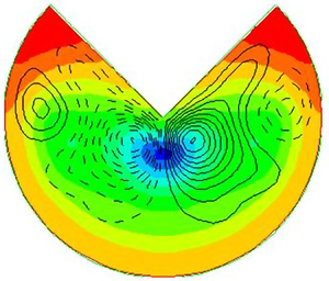
Let us try to apply the outlined recipe to some specific cases. Figures 6 and 7 show the pressure distributions and secondary flow streamlines (stream function isolines) in pipes with a cross-section in the form of a circular sector with apex angle of  $90\,^\circ$ and
 $270\,^\circ$, obtained in direct numerical simulations (DNS) at Reynolds number
 $Re_{Dh}=U_bD_h/\nu \approx 2800$ (N. Nikitin, unpublished paper). Here,
 $U_b$ is the bulk velocity,
 $D_h$ is the hydraulic diameter (
 $D_h=4S/P$, where
 $S,P$ are the cross-section area and the wetted perimeter).
(a) Mean pressure distribution and (b) streamlines of secondary flow in a pipe with a cross-section in the form of a circular sector with an apex angle of  $90\,^\circ$.

(a) Mean pressure distribution and (b) streamlines of secondary flow in a pipe with a cross-section in the form of a circular sector with an apex angle of  $270\,^\circ$.

A priori analysis of the  $90\,^\circ$ apex angle pipe (figure 6) leads to the following conclusions. In the three cross-section interior corners
 $A, B, B'$, the pressure reaches the local maximum for the reasons described above. On straight sections
 $AB$ and
 $AB'$ there must be points of local pressure minimum, we denote them by
 $C$ and
 $C'$. In these areas, there is no change in the curvature of the boundary or other circumstances that make us assume the presence of other extrema. In the middle of the arc
 $BB'$ at the point
 $D$, by virtue of symmetry, there must be a pressure extremum. Since this point is located between two maxima, it is probably a minimum. It remains to connect the pressure extrema points in accordance with the rule of figure 5 with no mutual intersections of the lines inside the pipe, to get an approximate picture of the secondary flow streamlines. In the present case, the supposed secondary flow is qualitatively equivalent to the flow in a tube of triangular cross-section (Prandtl Reference Prandtl1926). The fluid from the central region of the pipe moves to the points of local pressure maximum located at the vertices of the three corners
 $B, B '$ and
 $A$. From the corners, the fluid spreads along the walls towards the points
 $C, C '$ and
 $D$. From these points, the fluid flows back towards the centre of the pipe. The DNS results confirm in general the prediction made in terms of the pressure distribution along the perimeter (figure 6a) and the shape of the streamlines (figure 6b).
Let us now turn to a pipe with an apex angle of  $270\,^\circ$. At the corner points, we assume pressure extrema. At the inner corners
 $B$ and
 $B'$ there should be local maxima and in the outer corner
 $A$, a local minimum. Note that the pressure behaviour is considered only along the perimeter. A local minimum at point
 $A$ means that the pressure is higher on the surrounding sections of the boundary, but does not mean that the pressure will necessarily increase at the surrounding points inside the pipe. In the middle of the arc
 $BB'$, by virtue of symmetry, there must be a local extremum. However, the type of this extremum is not obvious in this case. The pressure behaviour at this point
 $D$ is less determined by the distant corners
 $B, B'$ than by the corner
 $A$. The direction of the convexity of the fluctuation trajectories in the vicinity of point
 $A$ coincides with the convexity of the boundary at point
 $D$, which can manifest itself in a certain increase in pressure in this point compared with the surrounding sections of the arc
 $BB'$. Thus, we can assume a local pressure maximum at point
 $D$, which means that local minima appear at some intermediate points
 $C, C'$ on the arcs
 $BD$ and
 $B'D$. In this case, the secondary flow along the boundary has a direction from the corners
 $B, B'$ towards the corner
 $A$ and towards the points
 $C, C'$, as well as from the point
 $D$ towards the points
 $C, C'$. From the points of local minimum
 $C, C'$ and
 $A$, the fluid first moves out from the wall, and then in the direction of points
 $B, B'$ and
 $D$, respectively.
The described picture of the pressure distribution along the perimeter and the resulting topology of the secondary flow is confirmed by the DNS results presented in figure 7. Note that it was obtained on the basis of only one assumption, that the pressure at the point  $D$ has a local maximum. An alternative assumption about a local pressure minimum at this point gives a different picture. In this case, the secondary flow along the arcs
 $BD$ and
 $B'D$ is directed towards point
 $D$, and from it towards the centre of the pipe, where it meets the secondary flow from the point
 $A$, after which both flows spread out towards the corners
 $B, B'$. Although such a picture is not confirmed by the DNS results in the present case, it can be realized for other values of the Reynolds number or the value of the angle at the vertex
 $A$.
It is interesting that pressure distribution along the radius  $AD$ in figure 7(a) has a minimum at some intermediate point but not at the point
 $A$. The explanation for this fact is that the radial velocity fluctuations in the vicinity of the singular point
 $A$ have a very significant value so that the negative first term on the right-hand side of (2.4) outweighs the positive value of the second term associated with the effect of the curvature of the fluctuation trajectories. Note that the radial axis of the polar coordinates (figure 3), in this case, is directed towards the convexity of the fluctuation trajectories, i.e. from the corner to the central area of the pipe, and not vice versa, as in the case of the inner corners (figure 4a).
Let us consider several more cases known from the literature.
(i) Elliptical tube (Nikitin & Yakhot Reference Nikitin and Yakhot2005; Voronova & Nikitin Reference Voronova and Nikitin2006, Reference Voronova and Nikitin2007), figure 8(a). The maximum curvature of the wall is achieved at the ends of the larger diameter, so a relative increase in pressure
 $P^+$ arises there. Conversely, the minimum curvature of the wall and the reduced pressure $P^-$ correspond to the ends of a smaller diameter. Applying the rule of figure 5 one finds that at each quarter of the perimeter, the fluid moves along the wall from the ends of the larger diameter towards the ends of the smaller one. The fluid collects at the centre of the ellipse along the minor semiaxes and flows back towards the walls along the major semiaxes.
(ii) Rectangular duct with rounded corners (Vidal et al. Reference Vidal, Vinuesa, Schlatter and Nagib2017), figure 8(b). In the corner regions, where the curvature of the boundary is maximum, an increase in pressure
$P^+$ arises. As long as the rounding radius is less than the duct half-width $r < h$, there is a rectilinear section with a reduced pressure $P^-$ on the bottom wall. So the picture of the secondary flow qualitatively coincides with the case of non-rounded corners: the fluid from the outer flow moves towards the points of increased pressure in the corners from where it spreads along the walls in both directions to the zones of reduced pressure.(iii) Semicircular wall duct (Vidal et al. Reference Vidal, Vinuesa, Schlatter and Nagib2017, Reference Vidal, Vinuesa, Schlatter and Nagib2018), figure 8(c). With the disappearance of the flat section on the lower wall, the region of reduced pressure there also disappears. Accordingly, the flow along the wall in the direction of the vertical line of symmetry disappears as well, and instead of the four-vortex picture of the secondary flow, a two-vortex one arises.
(iv) Annular eccentric tube (Nikitin Reference Nikitin2006c; Nikitin, Wang & Chernyshenko Reference Nikitin, Wang and Chernyshenko2009), figure 9. The prediction of the shape of the secondary flow in the eccentric annular tube is not so obvious. Regarding the distribution of pressure along the walls, a priori, with a high degree of confidence, we can only assert that the pressure on the convex surface of the outer cylinder is greater than at the nearest point on the concave surface of the inner cylinder. The pressure distributions along the perimeter of the inner and outer cylinders obtained in the DNS Nikitin et al. (Reference Nikitin, Wang and Chernyshenko2009) are shown in figure 9(b). The positions of local pressure extrema at each boundary are marked in figure 9(a). The direction of fluid motion along the walls is consistent with the pressure distribution. Note that the range of pressure variation along the wall of the inner cylinder is twice as large as that along the outer cylinder. Considering that the length of the inner perimeter is half the outer one, the characteristic pressure gradient along the inner wall is four times greater than along the outer one. This is reflected by a noticeably higher intensity of the secondary flow along the surface of the inner boundary in the interval
$0.1 < s < 0.65$, where the fluid moves from a narrow to a wide gap. In the same direction, there is a weak movement along the outer cylinder. In the widest part of the gap $s<0.2$, the pressure change along the outer boundary stops and the secondary flow also disappears. In the narrow part of the gap $s>0.7$, the pressure drops with an increase in $s$ at both boundaries. In this part of the pipe, the fluid should move towards a narrow gap. On the outer cylinder, this is clearly seen in figure 9(a). On the inner one, it manifests itself in the form of separation of the streamline closest to the wall. Probably closer to the wall in this place there is a slight movement with the opposite direction not marked in the figure.


Schematic picture of secondary flows (a) in an elliptical pipe (Nikitin & Yakhot Reference Nikitin and Yakhot2005; Voronova & Nikitin Reference Voronova and Nikitin2006, Reference Voronova and Nikitin2007); (b) in a rectangular pipe with rounded corners (Vidal et al. Reference Vidal, Vinuesa, Schlatter and Nagib2017); (c) in a pipe with a semicircular wall (Vidal et al. Reference Vidal, Vinuesa, Schlatter and Nagib2017, Reference Vidal, Vinuesa, Schlatter and Nagib2018). Dashed lines correspond to clockwise rotation, solid lines to anticlockwise rotation. Additionally, the direction of rotation in the secondary flows is indicated by arrows. Areas with a local increase in pressure on the wall are denoted by  $P^+$ and areas with a reduced pressure by
 $P^-$.

Flow in an annular eccentric tube (Nikitin et al. Reference Nikitin, Wang and Chernyshenko2009). The upper half of the cross-section is shown. (a) Streamlines of the secondary flow; (b) mean pressure distributions along the perimeter of the inner (dashed line) and outer (solid line) cylinders. The coordinate  $s=0$ corresponds to the wide part of the gap,
 $s=1$, to the narrow one. Green dots on the cylinder walls point to the positions of the local pressure extrema
 $P^+$ and
 $P^-$.

4. Flow in an open channel
Let us now consider a turbulent flow in a rectangular channel, one of the walls of which is shear-free. We direct the  $y$ axis along the channel width and
 $z$ along the height (figure 10). Three walls are considered solid, and one,
 $z=h$, is free. Flows in open channels are studied intensively due to their obvious geophysical importance. Special attention is paid to secondary flows arising from the formation of roughness inhomogeneities at the channel bed (Tominaga et al. Reference Tominaga, Nezu, Ezaki and Nakagawa1989; Nezu & Nakagawa Reference Nezu and Nakagawa1993; Pan & Banerjee Reference Pan and Banerjee1995; Albayrak & Lemmin Reference Albayrak and Lemmin2011; Yang, Tan & Wang Reference Yang, Tan and Wang2012; Stoesser, McSherry & Fraga Reference Stoesser, McSherry and Fraga2015). Under natural conditions, these flows, covering the entire thickness of the flow, significantly affect the gas and heat exchange, self-aeration on the free surface, and the transfer of bottom sediments (Nezu & Nakagawa Reference Nezu and Nakagawa1993).
Scheme of secondary flows in an open channel (Nezu & Nakagawa Reference Nezu and Nakagawa1993).

In smooth channels, the most intense secondary flows arise in the corner regions, where the sidewalls intersect with the horizontal bottom (Nezu & Nakagawa Reference Nezu and Nakagawa1993). These flows have the form of two cells, lower and upper, with the opposite direction of fluid rotation (figure 10). The motion in the upper cell is directed from the sidewall along the free surface; it is more intense than the flow in the lower cell. With distance from the sidewall, the intensity of the secondary flow weakens and disappears at a distance of  $\sim 3h$ (
 $h$ is the channel depth) (Nezu & Rodi Reference Nezu and Rodi1985). Note that the described picture of the secondary flow in an open channel differs from the secondary flow in a rectangular duct in which not one, but two pairs of vortices are observed at each of the sidewalls.
A detailed experimental and numerical study of the flow in the corner between the free boundary and the solid wall (Grega et al. Reference Grega, Wey, Leighton and Neves1995) revealed the presence of a less intense ‘internal’ secondary vortex, in which the motion is directed towards the corner along the free boundary. Investigation of the mechanisms of momentum and energy transfer in this area is carried out in Broglia, Pascarelli & Piomelli (Reference Broglia, Pascarelli and Piomelli2003).
The conditions for the formation of secondary flows in an open channel differ from the case of a channel with solid walls in that there are tangential velocity fluctuations on the free surface, which are absent on a solid wall (normal fluctuations associated with the deformation of the free surface are neglected in this work). For the reasons stated above, in each of the four cross-section corners, a zone of increased pressure should appear and a pressure gradient displacing the fluid along the walls out of the corner. Near solid walls, where there are no Reynolds stress forces that could counteract the pressure force, the fluid must move away from the corner. However, on a free surface, the direction of motion, generally speaking, can be different and is determined by the competition between the pressure and Reynolds stress gradients. If, as a result of this competition, the pressure force wins, then a secondary flow will arise, similar to the flow in a corner with solid walls, so that the liquid spreads along the walls to both sides of the corner. If the pressure force is inferior, then the fluid in the secondary flow will move along the free surface towards the corner and be carried down along the solid wall, i.e. in the upper corner, a single vortex picture of the secondary flow appears, corresponding to the ‘internal vortex’ (Grega et al. Reference Grega, Wey, Leighton and Neves1995; Broglia et al. Reference Broglia, Pascarelli and Piomelli2003). In any of the two possible scenarios, in the vicinity of the upper corners, the liquid must move downward along the solid sidewall, which contradicts the secondary flow pattern, according to which the liquid flows to the upper corner along the sidewall and is carried away to the centre of the channel along the free surface (Nezu & Nakagawa Reference Nezu and Nakagawa1993). To study the details of the secondary flow in the region between a free surface and a solid wall from the point of view of the proposed mechanism, in this work, DNS of turbulent flow in a rectangular channel with a free boundary is carried out within the framework of the full Navier–Stokes equations.
4.1. Problem formulation and solution method
The problem is solved in the formulation traditional for DNS of turbulent flows in channels. The Navier–Stokes equations for incompressible fluid,
 \begin{equation} \frac{{\partial} \boldsymbol{u}}{{\partial} t}+(\boldsymbol{u}\boldsymbol{\cdot}\boldsymbol{\nabla})\boldsymbol{u}={-}\boldsymbol{\nabla} p+\nu\nabla^2\boldsymbol{u},\quad \boldsymbol{\nabla}\boldsymbol{\cdot}\boldsymbol{u}=0 ,\end{equation}
are solved with the periodicity conditions along the flow, no-slip boundary conditions on the bottom and sidewalls, and the condition of a free wall on the upper boundary,
 \begin{equation} \frac{{\partial} u}{{\partial} z}=\frac{{\partial} v}{{\partial} z}=w=0,\quad z=1. \end{equation}
All quantities are presented in dimensionless form. The depth of the channel  $h$ is taken as the length scale, and the bulk flow velocity
 $U_b$ is taken as the velocity scale. Normalization to wall (viscous) scales of velocity
 $u_\tau =\overline {\tau }_w/\rho$ and length
 $l_\tau =\nu /u_\tau$, where
 $\overline {\tau }_w$ is the mean friction on the solid walls of the channel,
 $\rho$ and
 $\nu$ are the density and kinematic viscosity of the fluid, denoted by the superscript ‘
 $+$’. The motion is driven by a longitudinal pressure gradient. The flow rate is kept constant.
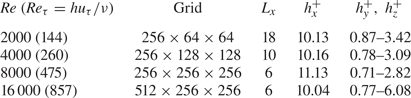
For the numerical solution of the problem, the algorithm of Nikitin (Reference Nikitin2006b) is used, which combines a finite-difference conservative scheme of the second order for the approximation in space and a semi-implicit third-order method of Nikitin (Reference Nikitin2006a) for integration in time. For presentation in this work, we selected the simulation results obtained in a channel with a cross-section of 4:1. The list of simulation parameters, including the values of the Reynolds numbers  $Re=U_b h/\nu$ and
 $Re_\tau =u_\tau h/\nu$, the dimensions of the computational domain (
 $W$ is the channel width,
 $L_x$ is the longitudinal period), sizes of grid cells
 $h_x, h_y, h_z$ in each spatial direction are given in table 1. The selected mesh sizes are adequate for reliable reproduction of the main statistical characteristics of the calculated flow. The results of simulations performed for other channel sizes and different Reynolds numbers confirm the qualitative conclusions presented in this work.
Simulation parameters.

Starting from some random initial conditions, the problem is integrated in time until the solution reaches a statistically stationary regime. After that, the equations continue to be integrated with the parallel set of statistics. Along with averaging over time, averaging is carried out over a homogeneous longitudinal coordinate. The resulting average fields depend only on the transverse coordinates  $(y, z)$. Figure 11 shows the secondary flow streamlines (stream function field) obtained as a result of averaging over
 $t$ and
 $x$. For reasons of symmetry, for long-term averaging, all fields should be symmetric about the line of symmetry
 $y = W/2$. The streamline shapes in the two symmetrical halves of the channel in figure 11 are close not only qualitatively, but also quantitatively. This indicates that the selected time-averaging period is sufficient for reliable averaging. The fields shown below were obtained using additional averaging over two symmetric halves of the channel cross-section. Mean values obtained in this way are indicated by overlines.
Secondary flow streamlines with no averaging about the line of symmetry  $y=W/2$.

4.2. Secondary flows in an open channel
The shape of the secondary flow streamlines in the vicinity of the upper corners (figure 11) confirms the assumption of the presence of secondary vortices and gives an answer to the question about their number posed at the beginning of § 4. Of the two listed probable scenarios, the second one is realized, which is consistent with the results of Grega et al. (Reference Grega, Wey, Leighton and Neves1995) and Broglia et al. (Reference Broglia, Pascarelli and Piomelli2003) with the formation of a single-vortex motion in the upper corners. The fluid goes down along the sidewall at the upper corners and does not rise up, as in the picture in Nezu & Nakagawa (Reference Nezu and Nakagawa1993). The presence of secondary vortices in the upper corners confirms the validity of the assumption about the existence of local pressure maxima in these regions of the channel.
The streamlines of the secondary flow together with the mean pressure field are shown in figure 12(a). Hereinafter, only the left of the two symmetrical halves of the channel is shown. As predicted, there is a pressure increase in each of the cross-sectional corners, including the upper one. The pressure difference over the channel cross-section is  $0.011(\times U_b^2$). The zone of increased pressure at the lower corner is noticeably larger in size than at the upper one. This is explained by the fact that the curvature of the fluctuation trajectories in the lower part of the channel occurs at a greater distance from the solid lower wall than in the upper part of the channel near the free boundary. The maximum pressure, however, is reached precisely in the upper corner. As will be shown below, the anomalous increase in pressure in this place is associated with a peculiarity of the flow in the region where the solid and free surfaces meet.
(a) Mean pressure field and streamlines of secondary flow; (b) isolines of mean longitudinal velocity.

On the free surface near the wall,  $0.017 < y \lesssim 0.2$, the action of the Reynolds stresses is directed towards the wall and exceeds the action of the pressure gradient, due to which the fluid in this section moves towards the corner and a single upper corner vortex is formed. The features of the balance of forces in the immediate vicinity of the corner point,
 $y < 0.017$, are described below. In other respects, the picture of the secondary flow is consistent with the traditional concept: most of the channel cross-section is occupied by two intense vortices that are generated in the lower corner and penetrate into the flow for a long distance. The contours of the mean longitudinal velocity
 $U(y,z)$ are shown in figure 12(b). They have characteristic features reflecting the effect of secondary flow. In the lower and upper corners these are the characteristic bulges towards the corners. The main feature inherent in the flow in open channels is an increase in the velocity under the free surface in the central part of the channel. The explanation of this effect is the surface transfer of fluid with a low momentum from the coastal zones towards the centre of the channel, carried out by a secondary flow.
Figure 13(a,b) present the intensity of transverse velocity fluctuations  $\sqrt {\overline {v'^2}+\overline {w'^2}}$ and the velocity of secondary flow
 $\sqrt {V^2+W^2}$. Transverse fluctuations near solid walls are noticeably more intense than at the free surface. However, the secondary flow which is generated by transverse fluctuations reaches the highest velocity precisely on the free surface. The intensity of the secondary flow is significantly higher than in a rectangular duct with solid walls. In the latter, the maximum velocity is reached in the near-wall region of the secondary vortices and has a value of approximately 1.5 % of the bulk velocity (Hoagland Reference Hoagland1960; Gavrilakis Reference Gavrilakis1992; Nikitin Reference Nikitin1997), while in the studied flow it reaches 2.5 % near the solid walls and 5 % on the free surface.
(a) Intensity of transverse velocity fluctuations  $\sqrt {\overline {v'^2}+\overline {w'^2}}$ (five contours with increments of 0.2); (b) isolines of the secondary flow velocity
 $\sqrt {V^2+W^2}$ (five contours with increments of 1 % of
 $U_b$).

Figure 14 shows the distributions along the free surface of the horizontal component of the secondary flow velocity  $V$, as well as all terms of (1.6), which explain in detail the mechanisms of vortex formation in the upper corner and intensification of the secondary flow on the free surface. The
 $y$ coordinate is given on a logarithmic scale, for more detailed disclosure of details in the immediate vicinity of the sidewall. The fluid moves towards the wall (
 $V <0$) at
 $y <0.21$ and away from the wall at larger
 $y$. The main driving force acting away from the corner is the pressure gradient
 $-{\partial } P/{\partial } y$, which is positive everywhere, except for a small section
 $1.1 < y < 1.2$. The pressure gradient decreases with distance from the sidewall, but it behaves non-monotonically. The positions of its extrema are consistent with the extrema of the inertia force (convective terms in (1.6)). The latter is described by the expression
 $-V{\partial } V/{\partial } y$ (since
 $-W{\partial } V/{\partial } z = 0$ on the free surface) and changes sign at the zeros of the function
 $V (y)$ and of its derivative. On the segment
 $0 < y < 0.28$, the Reynolds stress force is negative (mainly due to the term
 $-{\partial }\overline {v'^2}/{\partial } y$) and competes with the force of the pressure gradient. As can be seen from the figure, the alternating force of inertia makes a noticeable contribution to this competition. In the
 $0.017 < y < 0.21$ segment the pressure forces loses and the fluid moves towards the corner. At larger
 $y$ the total force of pressure, inertia and Reynolds stresses becomes positive and the fluid moves towards the centre of the channel. For all values of
 $y$, the sum of the forces of pressure, inertia and Reynolds stresses is balanced by the force of viscous friction, marked in figure 14 by a solid line with round markers. On the segment
 $y>0.017$, the friction force is predictably directed against the motion. The dominant term is
 $\nu {\partial }^2 V/{\partial } z^2$, which expresses the change in friction between adjacent moving horizontal layers.
Secondary flow velocity and terms of (1.6) along the free surface,  $z=1$. Lines: 1,
 $V/2$; 2,
 $-{\partial } P/{\partial } y$; 3, Reynolds stresses force (right-hand side terms of (1.6)); 4, force of inertia (convective terms)
 $-V{\partial } V/{\partial } y-W{\partial } V/{\partial } z$; 5, viscous force
 $\nu ({\partial }^2 V/{\partial } y^2 + {\partial }^2 V/{\partial } z^2)$.

An interesting section is in the immediate vicinity of the wall  $y<0.017$, where, due to impermeability on the sidewall,
 $V, v'\to 0$, so that the inertial forces, the Reynolds stress forces, and the viscous term
 $\nu {\partial }^2V/{\partial } z^2$ tend to zero. The pressure gradient here, however, is finite and increases when approaching the wall. The action of the pressure gradient in this interval is balanced by the force of viscous friction, the direction of which coincides only in a single place with the direction of motion of the fluid. This interesting effect of the interaction of a solid and a free wall can be explained, for example, as follows. The viscous term in (1.6) can be written as
 $\nu ({\partial }^2 V/{\partial } y^2 + {\partial }^2 V/{\partial } z^2) = -\nu {\partial }\varOmega _x/{\partial } z$. Due to the absence of friction on the free surface
 $\varOmega _x = 0$ at
 $z = 1$, therefore the sign of the viscous term coincides with the sign of
 $\varOmega _x$ directly under the free surface. In the region of the upper left corner vortex
 $y<0.21$, the sign of
 $\varOmega _x$ is positive (anticlockwise rotation), therefore the viscous force is also positive. However, by virtue of the no-slip condition at
 $y = 0$,
 $\varOmega _x$ must change sign near the sidewall, which is what happens at
 $y<0.017$. Thus, the force of viscous friction changes sign and balances the force of the pressure gradient.
The distribution of the mean longitudinal vorticity over the channel cross-section is shown in figure 15(a). In figure 15(b), a region is highlighted adjacent to the upper corner, demonstrating the fine structure of  $\varOmega _x$ with a sign change near the solid wall at
 $y<0.017$. Everywhere at
 $y>0.21$ under the free surface
 $\varOmega _x$, and hence the force of viscous friction is negative, which means that the sum of all other forces is positive. In the absence of friction on the upper surface, a significant secondary flow velocity is required to balance these forces by friction against the underlying layers of the fluid. This is the reason for the formation of intensive secondary flow with a velocity of up to 5 % of
 $U_b$.
Distribution of the mean longitudinal vorticity  $\varOmega _x$ over the channel cross-section. Negative values are shown with dashed lines.

5. Secondary flows in a channel with two adjacent free boundaries
The study of flow in a channel with a free boundary revealed several interesting properties of secondary flows. Based on the formulated principle of the formation of secondary flows, the possibility of a secondary flow in the form of a single vortex in the region between a solid wall and a free surface in the cross-sectional plane (Grega et al. Reference Grega, Wey, Leighton and Neves1995; Broglia et al. Reference Broglia, Pascarelli and Piomelli2003) was predicted. The fact of the appearance of a secondary vortex in this place is due to the presence of a no-slip solid wall, and the appearance of only one vortex, and not two, is a distinctive feature of the interaction between a solid wall and a free boundary. The question of the possibility and peculiarities of the formation of secondary flows in the corners between two free boundaries looks interesting, where a solid wall, as an important element of the mechanism of a secondary flow formation, is absent.
Imagine that the channel has two adjacent free walls. The cross-section in such a channel has one corner bounded by solid walls, in which a standard two-vortex secondary flow should arise. One-vortex secondary structures, described in the previous section, are likely to be expected at two corners between the solid and free boundaries. Let us try, based on the results of the previous sections, to predict the structure of the secondary flow in the fourth corner bounded by two free boundaries. Here, as in all other corners, one should expect a zone of increased pressure, and, consequently, a pressure gradient displacing the liquid along the free boundaries. Since Reynolds stresses now act along each of the adjacent free boundaries, the question of the direction of the secondary flow is determined by the competition of forces. In the channels with a square cross-section, considered in this work, the mean flow is symmetric about the corner bisector. So that if the pressure gradient wins, then a two-vortex flow arises with spreading along the walls, similar to the flow in a corner with solid walls. If the pressure gradient is inferior, then the motion along the walls will occur towards the apex of the corner, followed by the outflow of the fluid along the bisector.
A channel with two free boundaries is difficult to implement experimentally, but it can be simulated numerically. Table 2 shows the parameters of four simulations carried out in a square channel with two adjacent free boundaries. All values are normalized to the channel width  $h$ and the bulk flow velocity
 $U_b$. The viscous scales are determined by the mean friction on solid walls. The boundaries
 $y = 0$ and
 $z = 0$ are considered solid, and the boundaries
 $y = 1$ and
 $z = 1$ are considered free. Averaging is carried out over time, longitudinal coordinate
 $x$ and two halves of the cross-section, symmetric about the diagonal
 $z = y$.
Simulation parameters.

Figure 16 shows the mean pressure fields and streamlines of the secondary flows obtained in all four simulations. With some quantitative differences, the qualitative structure of the presented fields is the same for all Reynolds numbers. At all four corners of the cross-section, there is a zone of increased pressure associated with the curvature of the fluctuation trajectories. Secondary vortices originating in the lower-left corner near the solid walls are carried away towards the free walls, where they are accelerated by forces acting along the free surface. At the smallest Reynolds number  $Re = 2000$, the secondary flow rate on the free surface is small, only approximately 1.2 %, but already at
 $Re = 4000$ it increases to 4 % and reaches 5.5 % at
 $Re = 8000$ and
 $16\,000$.
Mean pressure fields and secondary flow streamlines in a channel with two shear-free boundaries: (a)  $Re = 2000$, (b)
 $Re = 4000$, (c)
 $Re = 8000$, (d)
 $Re = 16\,000$. The boundaries
 $y = 0$ and
 $z = 0$ are solid, and the boundaries
 $y = 1$ and
 $z = 1$ are free.

The velocity of the secondary flow in single vortices in the corners between solid and free walls remains approximately constant at a level of 2.3 %–2.5 % for all  $Re$. The size of these vortices decreases with increasing
 $Re$. However, their characteristic diameter
 $D$, expressed in viscous units, on the contrary, slightly increases from
 $D^+\approx 50$ at
 $Re = 2000$ to
 $D^+\approx 84$ at
 $Re = 16\,000$. The coordinate of the point where the direction of motion of the secondary flow changes on the free surface is taken as the diameter
 $D$. At a close point, changes the sign of the Reynolds stresses force as well (line 3 in figure 14). As noted above, this force in the corner region on the free surface
 $z=1$ is largely determined by the gradient of the square of normal velocity fluctuations,
 $-{\partial }\overline {v'^2}/{\partial } y$. In near-wall turbulent flows, the intensity of normal velocity fluctuations increases with distance from the wall, after which it begins to decrease. At low Reynolds numbers (
 $Re_\tau \approx 180$), the maximum
 $\overline {v'^2}$ is reached at
 $y^+\approx 50$ (Kim, Moin & Moser Reference Kim, Moin and Moser1987). With an increase in
 $Re$, the distance from the wall to the maximum point increases to
 $y^+\approx 100$ at
 $Re_\tau = 1000$ and somewhat more at larger
 $Re_\tau$ (Lee & Moser Reference Lee and Moser2015). Thus, the diameter of the corner vortex
 $D^+$, increasing with increasing
 $Re$, probably does not exceed a value of one or a few hundred viscous lengths even at very high values of the Reynolds number. This explains the fact that the presence of an upper corner secondary vortex in open channels was not previously recorded in experiments carried out, as a rule, under conditions close to natural ones at high Reynolds numbers. For example, in the Jing, Yang & Chen (Reference Jing, Yang and Chen2019) experiments in a channel 30 cm wide, the diameter of the upper corner vortex, according to our estimates, should be approximately 3 mm.
The most interesting thing is that, contrary to forecasts, in the upper right corner, between two free surfaces, there is no noticeable secondary flow generation. That is, neither the first nor the second predicted scenarios are realized. This is possible only if the action of the Reynolds stress forces is balanced by the pressure gradient, i.e. the Reynolds stress forces, in this case, are potential and do not form vorticity. To clarify what has been said, we present (1.6) and (1.7) in a modified form as follows:
 \begin{gather} \left.\begin{array}{c@{}} V\dfrac{{\partial} V}{{\partial} y}+W\dfrac{{\partial} V}{{\partial} z}-\nu\left(\dfrac{{\partial}^2 V}{{\partial} y^2}+\dfrac{{\partial}^2 V}{{\partial} z^2}\right)+\dfrac{{\partial} (P-Q)}{{\partial} y}=f_y-\dfrac{{\partial} Q}{{\partial} y},\\ f_y={-}\dfrac{{\partial}\overline{v'^2}}{{\partial} y}-\dfrac{{\partial}\overline{v'w'}}{{\partial} z}, \end{array}\right\} \end{gather}
 \begin{gather} \left.\begin{array}{c@{}} V\dfrac{{\partial} W}{{\partial} y}+W\dfrac{{\partial} W}{{\partial} z}-\nu\left(\dfrac{{\partial}^2 W}{{\partial} y^2}+\dfrac{{\partial}^2 W}{{\partial} z^2}\right)+\dfrac{{\partial} (P-Q)}{{\partial} z}=f_z-\dfrac{{\partial} Q}{{\partial} z},\\ f_z={-}\dfrac{{\partial}\overline{v'w'}}{{\partial} y}-\dfrac{{\partial}\overline{w'^2}}{{\partial} z}. \end{array}\right\} \end{gather}
Here  $Q$ is the pressure caused by the Reynolds stress force
 $f = (\,f_y, f_z)$. The scalar field
 $Q$, which we will call the fluctuation pressure, is found from the solution of the Neumann problem for the Poisson equation,
 \begin{equation} \nabla^2 Q=\boldsymbol{\nabla}\boldsymbol{\cdot}\boldsymbol{f}, \quad \left.\frac{{\partial} Q}{{\partial} n}\right|_\varGamma=\boldsymbol{f}\boldsymbol{\cdot}\boldsymbol{n}. \end{equation}
Here  $\boldsymbol {n}$ is the outward normal at the boundary of the pipe cross-section
 $\varGamma$. In this representation, the pressure
 $P$ is divided into the sum of
 $Q$ and
 $P-Q$, the latter being determined by the secondary flow. The Reynolds equations in the form (5.1), (5.2) are more convenient for the analysis of secondary flows, since not the Reynolds stress force
 $\boldsymbol {f}$ itself, but only its vortical part obtained by subtracting the gradient
 $Q$ is the real cause of the occurrence secondary flow. In particular, the secondary flow will not arise at all even if the force
 $\boldsymbol {f}$ is not zero, but is potential.
Figures 17–19 show the vector fields of the Reynolds stress force  $\boldsymbol {f}$, minus gradient of the fluctuation pressure
 $Q$ and their sum in the vicinity of three corners, where the boundaries of different type are intersect: two no-slip walls
 $y = 0$ and
 $z = 0$ (figure 17); no-slip wall
 $y = 0$ and a free boundary
 $z = 1$ (figure 18); and two free boundaries
 $y = 1$ and
 $z = 1$ (figure 19). The case of the maximum Reynolds number
 $Re = 16\,000$ is presented. Each figure shows a region of
 $0.12\times 0.12$ which is approximately
 $100\times 100$ viscous units at this
 $Re$.
Fields of the  $(\textit {a})$ Reynolds stress force
 $\boldsymbol {f}$,
 $(\textit {b})$ minus gradient of the fluctuation pressure
 $Q$,
 $(\textit {c})$ their sum in the vicinity of the intersection of two solid walls
 $y = 0$ and
 $z = 0$. Here
 $Re = 16\,000$. The size of the vectors in panel (c) has been increased by 10 times compared with panels (a) and (b).

Fields of the (a) Reynolds stress force  $\boldsymbol {f}$, (b) minus gradient of the fluctuation pressure
 $Q$, (c) their sum in the vicinity of the intersection of solid wall
 $y = 0$ and free boundary
 $z = 1$. Here
 $Re = 16\,000$. The size of the vectors in panel (c) has been increased by 10 times compared with panels (a) and (b).

Fields of the (a) Reynolds stress force  $\boldsymbol {f}$, (b) minus gradient of the fluctuation pressure
 $Q$, (c) their sum in the vicinity of the intersection of two free boundaries
 $y = 1$ and
 $z = 1$. Here
 $Re = 16\,000$. The size of the vectors in panel (c) has been increased by 10 times compared with panels (a) and (b). The size of vectors on all panels is doubled compared with figures 17 and 18.

At first glance, the difference between the fields of the Reynolds stress force  $\boldsymbol {f}$ at different corners is small. In each case, the direction towards the corner point in the vicinity of the corner bisector and the direction normal to the nearest wall in other parts of the corner area dominate. The fields
 $-\boldsymbol {\nabla } Q$ are also close to each other, coinciding in many respects with the corresponding fields
 $\boldsymbol {f}$, taken with the opposite sign. One can only notice the presence of non-zero tangential components near the solid walls, which are absent in the fields
 $\boldsymbol {f}$. A significant difference between these fields at corners of different types is manifested only in their sum
 $\boldsymbol {f}-\boldsymbol {\nabla } Q$, the characteristic value of which in each case is an order of magnitude less than each of the terms. It is this small difference that determines the shape of the secondary flow caused. In the vicinity of two solid walls, this is a pair of symmetric vortices; in the vicinity of the intersection of a solid wall and a free boundary, this is a single vortex. Between two free boundaries, the fields
 $\boldsymbol {f}$ and
 $-\boldsymbol {\nabla } Q$ neutralize each other with an accuracy comparable to the calculation errors. Thus, we can conclude that the Reynolds stress force in this region is potential and does not produce a secondary flow. The secondary flow is preserved here only due to convection from distant regions of the cross-section.
6. Conclusion
A simple principle is formulated in this work, which makes it possible to explain and, in some cases, to predict the shape of secondary flows of Prandtl's second kind that arise in turbulent flows in straight pipes of non-circular cross-section. The secondary flows are consistent with the distribution of the mean pressure along the cross-sectional boundary. Fluid moves along the boundary from high to low mean pressure, since there are no Reynolds stress forces on the no-slip solid wall, and the pressure force can be balanced only by the viscous friction force acting opposite to the motion direction. Thus, the direction of secondary motion along the pipe perimeter can be determined by the location of the local mean wall pressure extrema. In some cases, the location of local pressure extrema can be established based on the analysis of the wall curvature. The fluctuation motion along a curved wall causes the pressure on the wall to change, the greater the change, the greater the curvature of the wall. On the convex boundary, an increase in pressure occurs, on the concave, on the contrary, a decrease in pressure occurs. The effectiveness of the proposed principle is demonstrated by a number of examples, such as the flows in a square duct, in an elliptical pipe, in pipes with a section in the form of a circular sector with an apex angle of  $90\,^\circ$ and
 $270\,^\circ$, in rectangular ducts with rounded corners, in an eccentric annular tube. In most cases, the approximate picture of secondary flows can be predicted a priori using only symmetry considerations and an analysis of the curvature of the cross-sectional boundary.
The conditions of the formulated principle are violated on a free surface, where, in addition to pressure, Reynolds stresses act on the fluid particles, and the result of their interaction is not known in advance. A turbulent flow in a rectangular channel is considered, in which one of the walls (upper) is free. A priori, it can be argued that in the upper corners of the cross-section, where the free surface intersects with the solid sidewalls, an increased pressure arises, which means that a secondary flow should form, directed downward along the solid sidewalls, regardless of the direction of motion along the free surface. This conclusion contradicts the previously existing concept of the picture of secondary flows in open channels (Nezu & Nakagawa Reference Nezu and Nakagawa1993), according to which the motion in the secondary flow is directed towards the upper corner along the solid wall and away from the corner along the free surface. The paper presents the results of DNS that confirm the predictions made, and agree with the results of Grega et al. (Reference Grega, Wey, Leighton and Neves1995) and Broglia et al. (Reference Broglia, Pascarelli and Piomelli2003) about the existence of an ‘internal’ secondary vortex in each of the corners between the solid wall and free boundary, the motion in which has a direction towards the corner along the free surface and from the corner downward along the sidewall. It should be noted that the characteristic size of the internal vortex is no more than 84 viscous units in the cases considered ( $Re_\tau <860$) and, probably, does not exceed one or a few hundred viscous units at large Reynolds numbers typical for laboratory experiments in open channels. The insignificant relative size of the upper corner secondary vortices probably explains the reason for the difficulty of detecting them in a laboratory experiment.
The presence of a solid wall with the no-slip condition is an important element of the described mechanism for the formation of secondary flows. There are no fluctuation forces on a no-slip solid wall, therefore, if a pressure gradient appears, it must certainly cause the fluid to move. In this regard, the question logically arises about the possibility of the formation of secondary flows at the corners between two free surfaces, on which there is no no-slipping. A channel with two adjacent free surfaces is difficult to implement in a laboratory experiment, but can be simulated numerically. A series of DNS of turbulent flows in a square channel with two solid and two free adjacent walls is performed for several Reynolds numbers from  $Re = 2000$ (
 $Re_\tau = 144$) to
 $Re = 16\,000$ (
 $Re_\tau = 857$). In the cross-section of such a channel, one corner is formed by two solid walls, two corners by one solid and one free, and one corner joins two free boundaries. The studies carried out made it possible to confirm and refine the results concerning the properties of secondary flows arising in the corner between the solid and free boundaries. The main result of these simulations is the discovery that the fluctuation forces in the vicinity of the corner between two free boundaries are potential, are neutralized by the pressure gradient, and therefore do not create a secondary flow.
The formulated mechanism for the formation of secondary flows in non-circular pipes intersects to some extent with Prandtl's explanation (Prandtl Reference Prandtl1926), according to which turbulent fluctuations along curved isovels (isotachs) in the vicinity of a corner produce a force acting towards the convexity of the isovel. Our explanation also involves the force arising from fluctuation motion along curved boundaries. However, there are several significant differences in our formulation. First, we are talking about the curvature of the fluctuation trajectories associated with the curvature of the boundary, and not isovels, which is not the same thing. The curvature of isovels is not always associated with the fluctuation trajectories and, therefore, with the appearance of fluctuation forces. An example of this is the velocity distribution under the free surface in figure 12(b) with a characteristic curvature of isovels, along which there is no particular fluctuation motion. Another example is the secondary flow in the vicinity of the corner between two free boundaries (figure 16). Here, the bulges of the isovels are directed out of the corner (not shown in the figure), while the fluctuation forces have an opposite direction, which is confirmed by a characteristic increase in pressure in the corner. The second essential aspect of the formulated mechanism is the presence of a solid wall. A fluctuation force, even acting in the direction of the corner, does not yet guarantee the occurrence of a secondary flow, since it can be neutralized by the pressure force, as it happens in the corner between two free boundaries. And only the presence of a solid wall, on which, due to the no-slip condition, there are no Reynolds stresses, ensures the formation of a secondary flow. On the whole, the results of this work provide a rational basis for understanding the reasons for the formation and prediction of the shape of secondary flows of Prandtl's second kind that arise in straight pipes of non-circular cross-section.
Acknowledgements
The research was carried out using the equipment of the shared research facilities of HPC computing resources at Lomonosov Moscow State University and computing resources of the federal collective usage center Complex for Simulation and Data Processing for Mega-science Facilities at NRC ‘Kurchatov Institute’ (ministry subvention under agreement RFMEFI62117X0016), http://ckp.nrcki.ru/.
Funding
The reported study was funded by RSF, project number 18-71-10075.
Declaration of interests
The author reports no conflict of interest.