1 Introduction
Magnetic topologies encountered in solar and stellar atmospheres or planetary magnetospheres are known to reconfigure in a few minutes leading to spectacular phenomena such as polar auroras or coronal mass ejections. Even in laboratory plasmas and tokamaks such rapid change of magnetic topology has also been observed. Although the physical processes underlying these phenomena are still a matter of debate (McPherron Reference McPherron1970; Kennel Reference Kennel and Kennel1996), they are likely due to kinetic instabilities developing in the current structures and contributing to the explosive release of magnetic energy into heat or beams of particles. In order to explain this drastic behaviour, much attention has been paid to magnetic reconnection and tearing instabilities for more than forty years (Coppi Reference Coppi1964; Coppi, Laval & Pellat Reference Coppi, Laval and Pellat1966; Galeev & Zelenyi Reference Galeev and Zelenyi1976; Silin, Büchner & Zelenyi Reference Silin, Büchner and Zelenyi2002; Birn & Priest Reference Birn and Priest2007). These studies often use a one-dimensional (1-D) slab model of current sheets with no perpendicular magnetic component to the central plane. In situ observations showed, however, that some substorm breakups might take place in the near-Earth region, closer than 10 Earth radii (
 $R_{E}$
), where the magnetic topology deviates strongly from a one-dimensional current sheet (Sergeev et al.
Reference Sergeev, Tanskanen, Mursula, Korth and Elphic1988; Lui et al.
Reference Lui, Lopez, Anderson, Takahashi, Zanetti, McEntire, Potemra, Klumpar, Greene and Strangeway1992; Shiokawa et al.
Reference Shiokawa, Shinohara, Mukai, Hayakawa and Cheng2005; Lui Reference Lui2016). The presence of a finite normal magnetic component
 $B_{z}$
changes the particle dynamics and a reconfiguration of the magnetic topology is more difficult to explain using standard reconnection models. Further measurements by THEMIS confirmed the presence of wave activity with periods ranging from seconds to minutes in the near-Earth region (Tang et al.
Reference Tang, Li, Angelopoulos, Mende, Glassmeier, Donovan, Russell and Lu2009; Kalmoni et al.
Reference Kalmoni, Rae, Watt, Murphy, Forsyth and Owen2015). Thus reconnection may not be the only mechanism at play during substorm events.
In the near-Earth region of the plasma sheet electrons are trapped in the 2-D magnetic bottle formed by the quasi-dipolar field. They bounce back and forth with periods ranging from a few seconds to one minute depending on the position of the mirror points. Electromagnetic perturbations oscillating within this range of period may enter into resonance with this bounce motion and this can modify the growth rate of potential instabilities. This wave/particle interaction is obviously a non-local process that can be addressed in the frame of kinetic theory alone. Tur, Louarn & Yanovsky (Reference Tur, Louarn and Yanovsky2010) proposed a complete integration of the Vlasov equation along the trajectories of the bouncing particles. This approach was also used previously in the context of fusion plasmas (Sharp, Berk & Nielsen Reference Sharp, Berk and Nielsen1979; Antonsen & Lane Reference Antonsen and Lane1980). An alternative way of treating this problem makes use of Hamiltonian theory (Littlejohn Reference Littlejohn1982). Fruit, Louarn & Tur (Reference Fruit, Louarn and Tur2013) reformulated the problem and added some algebraic corrections to the general calculation in Tur et al. (Reference Tur, Louarn and Yanovsky2010). The purpose of that study was to show that a 2-D current sheet with an untrapped (passing) electron population is stable regarding potential electrostatic perturbations. However, if the passing electron population is partly or totally removed from the system, the magnetic structure becomes violently unstable with a growth rate comparable to the mode frequency. This conclusion was interesting but the theory was restricted to the electrostatic perturbations only.
The present paper aims to complete the investigation. In Fruit et al. (Reference Fruit, Louarn and Tur2013) diamagnetic drift effects were not considered in order to concentrate on the analysis of the bounce effects. This is not optimal since spatial non-homogeneities are well known to trigger various drift instabilities (Hasegawa Reference Hasegawa1975). In the Earth magnetotail context, the cross-tail current is mainly produced by diamagnetic drift effects due to a density gradient along the tail. In a low
 $\unicode[STIX]{x1D6FD}$
regime, it is well known that a straight magnetic geometry with a perpendicular density gradient supports electromagnetic drift waves propagating perpendicular to both the magnetic field and the density gradient. These are called drift-Alfvén waves and they have been treated in various textbooks (Hasegawa Reference Hasegawa1975; Mikhailovskii Reference Mikhailovskii1998; Weiland Reference Weiland2012). The low-
 $\unicode[STIX]{x1D6FD}$
assumption means that parallel magnetic perturbations are neglected as well as the gradient/curvature drift of the particles. Neglecting finite Larmor radius effects and with
 $V_{i}\ll \unicode[STIX]{x1D714}/k_{\Vert }\ll V_{e}$
(
 $V_{\unicode[STIX]{x1D6FC}}$
denoting the thermal velocity of population
 $\unicode[STIX]{x1D6FC}$
), the dispersion relation for those modes is traditionally noted
 $(\unicode[STIX]{x1D714}-\unicode[STIX]{x1D714}_{e}^{\ast })(\unicode[STIX]{x1D714}^{2}-\unicode[STIX]{x1D714}_{i}^{\ast }\unicode[STIX]{x1D714}+k_{\Vert }^{2}c_{A}^{2})=0$
where
 $\unicode[STIX]{x1D714}^{\ast }$
means the drift particle frequency and
 $c_{A}$
is the Alfvèn velocity (Hasegawa Reference Hasegawa1975). These drift waves are destabilized by the introduction of a small ion–electron collision term or by kinetic effects such as Landau damping on the electron population. However, in a straight magnetic configuration where electrons are free to move along the field lines these unstable drift waves are not believed to play an important role in the magnetospheric context because ion Landau damping may constitute a stabilization mechanism at finite
 $\unicode[STIX]{x1D6FD}$
. Furthermore, the addition of a cold electron population may stabilize the electrostatic drift waves and its applicability to magnetospheric studies is put into question (Hasegawa Reference Hasegawa1975).
Following this line of thought, the electromagnetic drift-Alfvén wave theory deserves to be reconsidered with inclusion of the electron bounce motion in a magnetic bottle. Assessing the role of this electron bounce oscillation on the propagation proprieties of these drift wave constitutes an interesting issue that the present paper addresses. This article is merely a follow up to Fruit, Louarn & Tur (Reference Fruit, Louarn and Tur2017), which considers the electrostatic problem only. The main conclusion of this first study was a strong enhancement in the growth rate of the classical universal instability (electrostatic drift instability) due to the presence of bouncing electrons that enter into resonance with the waves. This is an interesting result in itself but the problem of substorm dynamics is fundamentally electromagnetic in nature. The present investigation focus on the electromagnetic case, considering a low
 $\unicode[STIX]{x1D6FD}$
configuration. It applies to the near-Earth magnetotail at distances lower than
 $12R_{E}$
, where the background magnetic field is high enough to neglect the compressional modes.
The paper is organized as followed: the general scheme of equations is summarized in § 2, much of the calculation was already reported thoroughly in Tur et al. (Reference Tur, Fruit, Louarn and Yanovsky2014) and all of the details are not reproduced here. The dispersion relation for the drift-Alfvén modes is then derived completely analytically in 3 with the help of a simplified model for the electron bounce motion and the slow ion approximation. A numerical integration of the dispersion relation and a physical discussion of the unstable modes ends the analysis.
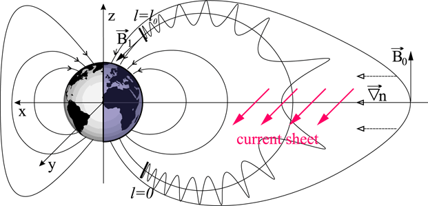
Geometry of magnetic field lines with length
 $l_{0}$
within a plasma sheet (dipolar model).

2 Theoretical formalism
2.1 Equilibrium state
The zero-order state is a 2-D current sheet in a low-
 $\unicode[STIX]{x1D6FD}$
approximation. It aims to model the near-Earth plasma sheet at equatorial distances between
 $8R_{E}$
and
 $12R_{E}$
where the magnetic topology deviates substantially from the dipole field but it is not yet shaped as a stretched tail configuration. The magnetic geometry is described in a rectilinear frame
 $(O,x,y,z)$
as shown in figure 1, where the
 $z$
-axis is south–north and the
 $x,y$
-axis is in the plane defined by the current. As the plasma sheet is assumed to be invariant along the
 $y$
direction, the particle distribution function depends only on the invariants of the particle dynamics, say the kinetic energy
 $E$
and the moment
 $P_{y}=mv_{y}+qA_{y}$
; taking into account a diamagnetic drift in the direction of the current
 $\boldsymbol{u}_{\unicode[STIX]{x1D6FC}}=u_{\unicode[STIX]{x1D6FC}}\boldsymbol{e}_{y}$
, a possible distribution function for each species
 $\unicode[STIX]{x1D6FC}$
is
 $$\begin{eqnarray}\displaystyle F_{0}^{(\unicode[STIX]{x1D6FC})}(\boldsymbol{r},\boldsymbol{v}) & = & \displaystyle n_{0}\left(\frac{m_{\unicode[STIX]{x1D6FC}}}{2\unicode[STIX]{x03C0}k_{B}T_{\unicode[STIX]{x1D6FC}}}\right)^{3/2}\exp \left(\frac{-m_{\unicode[STIX]{x1D6FC}}u_{\unicode[STIX]{x1D6FC}}^{2}}{2k_{B}T_{\unicode[STIX]{x1D6FC}}}\right)\nonumber\\ \displaystyle & & \displaystyle \times \,\exp \left(-\frac{E_{\unicode[STIX]{x1D6FC}}-u_{\unicode[STIX]{x1D6FC}}P_{y,\unicode[STIX]{x1D6FC}}}{k_{B}T_{\unicode[STIX]{x1D6FC}}}\right),\end{eqnarray}$$
where
 $m_{\unicode[STIX]{x1D6FC}}$
,
 $T_{\unicode[STIX]{x1D6FC}}$
,
 $q_{\unicode[STIX]{x1D6FC}}$
and
 $n_{0}$
are the mass, temperature, charge and density of species
 $\unicode[STIX]{x1D6FC}$
.
With a magnetic potential
 $\boldsymbol{A}=\unicode[STIX]{x1D6F9}(x,z)\boldsymbol{e}_{y}$
and introducing the thermal velocity for each species
 $V_{\unicode[STIX]{x1D6FC}}=\sqrt{2k_{B}T_{\unicode[STIX]{x1D6FC}}/m_{\unicode[STIX]{x1D6FC}}}$
, (2.1) can be rewritten as
 $$\begin{eqnarray}F_{0}^{(\unicode[STIX]{x1D6FC})}=\frac{n_{0}(\unicode[STIX]{x1D6F9})}{\unicode[STIX]{x03C0}^{3/2}V_{\unicode[STIX]{x1D6FC}}^{3}}\exp \left(-\frac{v_{x}^{2}+(v_{y}-u_{\unicode[STIX]{x1D6FC}})^{2}+v_{z}^{2}}{V_{\unicode[STIX]{x1D6FC}}^{2}}\right),\end{eqnarray}$$
with
 $n_{0}(\unicode[STIX]{x1D6F9})=n_{0}\exp (q_{\unicode[STIX]{x1D6FC}}u_{\unicode[STIX]{x1D6FC}}\unicode[STIX]{x1D6F9}/(k_{B}T_{\unicode[STIX]{x1D6FC}}))$
. Charge neutrality at equilibrium imposes the relation
 $$\begin{eqnarray}\frac{u_{i}}{k_{B}T_{i}}+\frac{u_{e}}{k_{B}T_{e}}=0\end{eqnarray}$$
for a plasma composed of only one type of ion (protons) and electrons.
In principle, the magnetic potential
 $\unicode[STIX]{x1D6F9}(x,y)$
is determined by Ampere’s law relating
 $\unicode[STIX]{x0394}\unicode[STIX]{x1D6F9}$
to the current density derived from (2.2). In a 2-D geometry the
 $\unicode[STIX]{x1D6F9}$
function cannot be determined exactly and only approximations have been derived (Lembege & Pellat Reference Lembege and Pellat1982, for example). A detailed expression for
 $\unicode[STIX]{x1D6F9}$
is however not required here because we simply adopt the magnetic configuration valid for
 $L\sim 8{-}10$
in the Earth magnetotail, where
 $L$
is a number of Earth radii equal to the distance of the farthest equatorial point of a given magnetic field line. Although invariance in
 $y$
is still considered in the central plasma sheet, field lines are assumed to reach acceleration regions above the ionosphere using a quasi-dipolar model. The length of the field line is denoted by
 $\ell _{0}$
. Using a dipolar model at
 $L=8$
, the magnitude of the magnetic field increases from approximately
 $B_{0}\sim 60~\text{nT}$
in the equatorial plane to
 $B_{1}+B_{0}\sim 60~\unicode[STIX]{x03BC}\text{T}$
at the ionosphere. A dimensionless stretching parameter
 $\unicode[STIX]{x1D700}=B_{0}/(B_{0}+B_{1})\simeq B_{0}/B_{1}\simeq 10^{-3}$
will be introduced later. The length of the field line is around
 $15.5R_{E}$
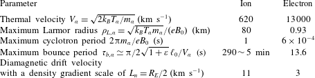
. From this geometry we can derive orders of magnitude for some important parameters concerning both ion and electron dynamics. They are listed in table 1.
Spatial and temporal scales characterizing particle dynamics in the Earth plasma sheet at
 $L=8$
, the total density
 $n_{0}=1\;\text{cm}^{-3}$
,
 $T_{i}=2~\text{keV}$
and
 $T_{e}=500~\text{eV}$
.

Diamagnetic drift velocity may be derived from a fluid point of view. Force equilibrium in the plasma sheet requires that
 $$\begin{eqnarray}u_{i}\simeq \frac{k_{B}T_{i}}{eB_{0}}\frac{\text{d}\ln n_{0}}{\text{d}x}.\end{eqnarray}$$
If
 $L_{n}=|\unicode[STIX]{x1D735}\ln n_{0}|^{-1}$
is the typical length scale of the density gradient along the tail, the normalized diamagnetic drift velocity reads
 $u_{d}=u_{i}/V_{i}=\unicode[STIX]{x1D70C}_{Li}/(\sqrt{2}L_{n})$
. From table 1 and with
 $L_{n}\sim R_{E}/2$
, the typical drift velocity is equal to
 $u_{d}\sim 0.02$
or
 $u_{i}\simeq 11~\text{km}~\text{s}^{-1}$
and
 $u_{e}\simeq 3~\text{km}~\text{s}^{-1}$
.
Finally, the natural field-aligned coordinates system
 $(\unicode[STIX]{x1D713},y,\unicode[STIX]{x1D712})$
defined by
 $$\begin{eqnarray}\boldsymbol{e}_{\unicode[STIX]{x1D712}}=\boldsymbol{B}/B,\quad \boldsymbol{e}_{\unicode[STIX]{x1D713}}=\unicode[STIX]{x1D735}\unicode[STIX]{x1D6F9}/|\unicode[STIX]{x1D735}\unicode[STIX]{x1D6F9}|,\quad \boldsymbol{e}_{y}=\boldsymbol{e}_{\unicode[STIX]{x1D712}}\times \boldsymbol{e}_{\unicode[STIX]{x1D713}}\end{eqnarray}$$
may sometimes be useful. Scale factors for this coordinate system are derived in appendix A where it is shown that these metric factors may be neglected in derivations since the parallel dimension
 $\ell _{0}$
is assumed to be much larger than the perpendicular wavelength, supposed to be of the order of the ion Larmor radius
 $\unicode[STIX]{x1D70C}_{Li}$
(
 $\unicode[STIX]{x1D70C}_{Li}/\ell _{0}\sim 1/1200$
).
2.2 Perturbed distribution functions
The above equilibrium state is assumed to be perturbed linearly by an electromagnetic wave described by the two potentials
 $\unicode[STIX]{x1D719}(\boldsymbol{r},t)$
and
 $A_{\Vert ,1}(\boldsymbol{r},t)$
. In the low
 $\unicode[STIX]{x1D6FD}$
approximation indeed, the perturbed magnetic field derives from a potential
 $\boldsymbol{A}_{1}=A_{\Vert ,1}\boldsymbol{e}_{\unicode[STIX]{x1D712}}$
with only a parallel component to the background field. We are mainly interested in drift waves propagating along the
 $y$
axis with perpendicular wavelength of the order of the ion Larmor radius, which is significantly smaller than the non-homogeneity scale in the
 $(x,z)$
plane. The perturbations are thus assumed to stay localized in the vicinity of the magnetic surface characterized by a given value
 $\unicode[STIX]{x1D6F9}_{0}$
. Following other studies based on the same assumption (Antonsen & Lane Reference Antonsen and Lane1980; Pellat Reference Pellat1990; Hurricane, Pellat & Coroniti Reference Hurricane, Pellat and Coroniti1994), we adopt a WKB formalism (as an approximation method for solving the linear differential equations) and choose a spatial dependence for the perturbed particle distribution function of the form
 $$\begin{eqnarray}f_{1}^{(\unicode[STIX]{x1D6FC})}(\boldsymbol{r},\boldsymbol{w},t)=\tilde{f}^{(\unicode[STIX]{x1D6FC})}(\unicode[STIX]{x1D6F9}_{0},\ell ,k,\unicode[STIX]{x1D714},\boldsymbol{w})\text{e}^{\text{i}(ky-\unicode[STIX]{x1D714}t)},\end{eqnarray}$$
where
 $\boldsymbol{w}$
is the particle velocity at time
 $t$
(to be distinguished from the velocity
 $\boldsymbol{v}$
at former times
 $t^{\prime }<t$
),
 $\ell$
the position of the particle along the field line at time
 $t$
and
 $k$
the wavenumber along the
 $y$
-direction. In the following, the amplitude will be noted simply
 $\tilde{f}^{(\unicode[STIX]{x1D6FC})}(\ell )$
, assuming implicit any reference to
 $\unicode[STIX]{x1D6F9}_{0}$
,
 $\unicode[STIX]{x1D714}$
,
 $k$
and
 $\boldsymbol{w}$
. Similarly the potentials read
 $$\begin{eqnarray}\unicode[STIX]{x1D719}_{1}(\boldsymbol{r},t)=\tilde{\unicode[STIX]{x1D719}}(\ell )\text{e}^{\text{i}(ky-\unicode[STIX]{x1D714}t)},\quad A_{\Vert ,1}(\boldsymbol{r},t)=\tilde{a}_{\Vert }(\ell )\text{e}^{\text{i}(ky-\unicode[STIX]{x1D714}t)}.\end{eqnarray}$$
The perturbed distribution function satisfies the linearized Vlasov equation
 $$\begin{eqnarray}\frac{\text{d}f_{1}^{(\unicode[STIX]{x1D6FC})}}{\text{d}t}=\frac{q_{\unicode[STIX]{x1D6FC}}}{m_{\unicode[STIX]{x1D6FC}}}\left[\unicode[STIX]{x1D735}\unicode[STIX]{x1D719}_{1}+\frac{\unicode[STIX]{x2202}\boldsymbol{A}_{1}}{\unicode[STIX]{x2202}t}-\boldsymbol{v}\times (\unicode[STIX]{x1D735}\times \boldsymbol{A}_{1})\right]\cdot \frac{\unicode[STIX]{x2202}F_{0}^{(\unicode[STIX]{x1D6FC})}}{\unicode[STIX]{x2202}\boldsymbol{v}},\end{eqnarray}$$
where
 $\text{d}/\text{d}t$
denotes the total time derivative. Using expression (2.2) for the unperturbed distribution function, an elegant solution for equation (2.8) may be formally written as (Tur et al.
Reference Tur, Fruit, Louarn and Yanovsky2014)
 $$\begin{eqnarray}\tilde{f}_{1}^{(\unicode[STIX]{x1D6FC})}(\boldsymbol{r},\boldsymbol{w},t)=\frac{qF_{0}^{(\unicode[STIX]{x1D6FC})}(\boldsymbol{r})}{k_{B}T_{\unicode[STIX]{x1D6FC}}}\left[-\tilde{\unicode[STIX]{x1D719}}(\boldsymbol{r},t)+\left(1-\frac{\unicode[STIX]{x1D714}_{\unicode[STIX]{x1D6FC}}^{\ast }}{\unicode[STIX]{x1D714}}\right)\tilde{g}^{(\unicode[STIX]{x1D6FC})}(\boldsymbol{r},\boldsymbol{w},t)\right],\end{eqnarray}$$
with
 $$\begin{eqnarray}\tilde{g}^{(\unicode[STIX]{x1D6FC})}=-\text{i}\unicode[STIX]{x1D714}\int _{-\infty }^{t}[\tilde{\unicode[STIX]{x1D719}}(\ell ^{\prime })-v_{\Vert }\tilde{a}_{\Vert }(\ell ^{\prime })]\text{e}^{\text{i}[\unicode[STIX]{x1D714}(t-t^{\prime })-k(y-y^{\prime })]}\,\text{d}t^{\prime },\end{eqnarray}$$
and
 $\unicode[STIX]{x1D714}_{\unicode[STIX]{x1D6FC}}^{\ast }=ku_{\unicode[STIX]{x1D6FC}}$
is the drift frequency. In this last integral,
 $\ell ^{\prime }=\ell (t^{\prime })$
,
 $y^{\prime }=y(t^{\prime })$
are explicit functions of time, corresponding to particle position along the unperturbed trajectory at time
 $t^{\prime }<t$
, the instant
 $t$
being the time of observation.
The integration of (2.10) for the trapped electron population relies on the double periodicity of the particle motion, namely the gyromotion and the bouncing between mirror points. To perform the computation a spatial form
 $[\tilde{\unicode[STIX]{x1D719}}(\ell ),\tilde{a}_{\Vert }(\ell )]$
must be prescribed for the potentials. As we are interested in perturbations confined within the plasma sheet, Dirichlet conditions may be chosen at the two ends of the field line for the electrostatic potential. Thus, if
 $\ell =0$
and
 $\ell =\ell _{0}$
pinpoint the boundaries, the potentials may be Fourier expanded as
 $$\begin{eqnarray}\displaystyle & \displaystyle \tilde{\unicode[STIX]{x1D719}}(\ell )=\mathop{\sum }_{n=1}^{\infty }\unicode[STIX]{x1D711}_{n}\sin \left(n\unicode[STIX]{x03C0}\frac{\ell }{\ell _{0}}\right), & \displaystyle\end{eqnarray}$$
 $$\begin{eqnarray}\displaystyle & \displaystyle \tilde{a}_{\Vert }(\ell )=\mathop{\sum }_{n=1}^{\infty }\unicode[STIX]{x1D6FC}_{n}\cos \left(n\unicode[STIX]{x03C0}\frac{\ell }{\ell _{0}}\right). & \displaystyle\end{eqnarray}$$
Calculation may be carried on for each mode, but the present analysis will restrict on the fundamental mode (
 $n=1$
) only. From (2.11)–(2.12) it is seen that
 $\tilde{\unicode[STIX]{x1D719}}$
and
 $\tilde{a}_{\Vert }$
have different symmetry properties along the field line. This is consistent with the expression of the magnetic and parallel electric fields
 $$\begin{eqnarray}\displaystyle & \displaystyle b_{\unicode[STIX]{x1D713},1}=\text{i}k_{y}\tilde{a}_{\Vert }\text{e}^{\text{i}(ky-\unicode[STIX]{x1D714}t)}, & \displaystyle\end{eqnarray}$$
 $$\begin{eqnarray}\displaystyle & \displaystyle e_{\Vert ,1}=\left[\text{i}\unicode[STIX]{x1D714}-\frac{\unicode[STIX]{x03C0}}{\ell _{0}}\frac{\unicode[STIX]{x1D711}_{1}}{\unicode[STIX]{x1D6FC}_{1}}\right]\tilde{a}_{\Vert }\text{e}^{\text{i}(ky-\unicode[STIX]{x1D714}t)}, & \displaystyle\end{eqnarray}$$
 $$\begin{eqnarray}\displaystyle & \displaystyle e_{y,1}=-\text{i}k_{y}\tilde{\unicode[STIX]{x1D719}}\text{e}^{\text{i}(ky-\unicode[STIX]{x1D714}t)}. & \displaystyle\end{eqnarray}$$
With this choice of boundary conditions a non-zero parallel electric field is generated at the ionospheric ends so the expected unstable modes may become important in the triggering process of auroras.
The time integration of (2.10) along the unperturbed particle orbit has been already exposed in detail in section III of Fruit et al. (Reference Fruit, Louarn and Tur2013). Here, we only summarize the main steps of the calculation which are also similar to the ones followed in Fruit et al. (Reference Fruit, Louarn and Tur2017).
(i) Integration along the gyromotion leads to the usual series of Bessel functions of the argument
 $\unicode[STIX]{x1D709}_{\unicode[STIX]{x1D6FC}}=kv_{\bot }/\unicode[STIX]{x1D714}_{c\unicode[STIX]{x1D6FC}}$
. Since the expected perturbations oscillate around the electron bounce frequency
$\unicode[STIX]{x1D714}_{be}$
, which is much lower than the electron gyrofrequency
$\unicode[STIX]{x1D714}_{ce}$
, the Bessel expansion may be restricted to the zero-order term and no electron cyclotron resonance is taken into account. This assumption should not hold for ions, however, since the ion gyrofrequency may sometimes be comparable to
$\unicode[STIX]{x1D714}_{be}$
. Nevertheless, we decide to discard them in this first approach of the drift-bounce interaction problem, and restrict the analysis to the situation where
$\unicode[STIX]{x1D714}\sim \unicode[STIX]{x1D714}_{be}\ll \unicode[STIX]{x1D714}_{ci}\ll \unicode[STIX]{x1D714}_{ce}$
which is consistent with values listed in table 1.
(ii) Integration along the electron bounce motion requires to specify a model for the parallel motion. To make things tractable analytically, this parallel motion is assumed to be purely harmonic. Noting by
$\unicode[STIX]{x1D707}$
the magnetic moment, the parallel velocity takes the simple form: (2.16)From this it is easy to derive the particle position along the field line$$\begin{eqnarray}\displaystyle v_{\Vert }(t)=v_{m}\sin \unicode[STIX]{x1D714}_{b}t=\sqrt{\frac{2(E-\unicode[STIX]{x1D707}B_{0})}{m_{e}}}\sin \left(\unicode[STIX]{x03C0}\frac{t}{\unicode[STIX]{x1D70F}_{b}}\right). & & \displaystyle\end{eqnarray}$$
(2.17)and two equivalent expressions for the magnetic field:$$\begin{eqnarray}\ell (t)=\frac{\ell _{0}}{2}\left[1-\sqrt{\frac{E-\unicode[STIX]{x1D707}B_{0}}{\unicode[STIX]{x1D707}B_{1}}}\cos \unicode[STIX]{x1D714}_{b}t\right],\end{eqnarray}$$
(2.18)$$\begin{eqnarray}\displaystyle B(\ell ) & = & \displaystyle B_{0}+B_{1}\left(\frac{2\ell }{\ell _{0}}-1\right)^{2}\end{eqnarray}$$
(2.19)$$\begin{eqnarray}\displaystyle & = & \displaystyle B_{1}\left[\frac{E+\unicode[STIX]{x1D707}B_{0}}{2\unicode[STIX]{x1D707}B_{1}}+\frac{E-\unicode[STIX]{x1D707}B_{0}}{2\unicode[STIX]{x1D707}B_{1}}\cos 2\unicode[STIX]{x1D714}_{b}t\right].\end{eqnarray}$$
The bounce period is then given by
(2.20)It depends only on$$\begin{eqnarray}\unicode[STIX]{x1D70F}_{b}=\unicode[STIX]{x03C0}\frac{\ell _{0}}{2}\sqrt{\frac{m_{e}}{2\unicode[STIX]{x1D707}B_{1}}(1+\unicode[STIX]{x1D700})}.\end{eqnarray}$$
$\unicode[STIX]{x1D707}$
and not on the energy of the particle. This result comes from the initial assumption of harmonic motion. More complex parallel motions should lead to a more realistic relationship
$\unicode[STIX]{x1D70F}_{b}(E,\unicode[STIX]{x1D707})$
but a numerical integration would likely be necessary.From this simple model describing the electron parallel bounce motion, however, it is possible to compute analytically the integral (2.10) and one gets (see (61) and (62) in Tur et al. (Reference Tur, Fruit, Louarn and Yanovsky2014)):
(2.21)$$\begin{eqnarray}\displaystyle g_{+}^{(e)} & = & \displaystyle \unicode[STIX]{x1D711}_{1}\left[J_{0}(\unicode[STIX]{x1D701})-J_{2}(\unicode[STIX]{x1D701})\left(\frac{\unicode[STIX]{x1D714}}{\unicode[STIX]{x1D714}+2\unicode[STIX]{x1D714}_{b}}+\frac{\unicode[STIX]{x1D714}}{\unicode[STIX]{x1D714}-2\unicode[STIX]{x1D714}_{b}}\right)\cos 2\unicode[STIX]{x1D714}_{b}t\right]\nonumber\\ \displaystyle & & \displaystyle -\,\text{i}\frac{v_{m}}{2}\unicode[STIX]{x1D6FC}_{1}J_{1}(\unicode[STIX]{x1D701})\left(\frac{\unicode[STIX]{x1D714}}{\unicode[STIX]{x1D714}+2\unicode[STIX]{x1D714}_{b}}-\frac{\unicode[STIX]{x1D714}}{\unicode[STIX]{x1D714}-2\unicode[STIX]{x1D714}_{b}}\right)\cos 2\unicode[STIX]{x1D714}_{b}t,\end{eqnarray}$$
(2.22)with$$\begin{eqnarray}\displaystyle g_{-}^{(e)} & = & \displaystyle \text{i}\unicode[STIX]{x1D711}_{1}J_{2}(\unicode[STIX]{x1D701})\left(\frac{\unicode[STIX]{x1D714}}{\unicode[STIX]{x1D714}+2\unicode[STIX]{x1D714}_{b}}-\frac{\unicode[STIX]{x1D714}}{\unicode[STIX]{x1D714}-2\unicode[STIX]{x1D714}_{b}}\right)\sin 2\unicode[STIX]{x1D714}_{b}t\nonumber\\ \displaystyle & & \displaystyle -\,\frac{v_{m}}{2}\unicode[STIX]{x1D6FC}_{1}J_{1}(\unicode[STIX]{x1D701})\left(\frac{\unicode[STIX]{x1D714}}{\unicode[STIX]{x1D714}+2\unicode[STIX]{x1D714}_{b}}+\frac{\unicode[STIX]{x1D714}}{\unicode[STIX]{x1D714}-2\unicode[STIX]{x1D714}_{b}}\right)\sin 2\unicode[STIX]{x1D714}_{b}t,\end{eqnarray}$$
$\unicode[STIX]{x1D701}=\unicode[STIX]{x03C0}/2\sqrt{(E-\unicode[STIX]{x1D707}B_{0})/\unicode[STIX]{x1D707}B_{1}}$
. To get these expressions we have inserted the particle position
$\ell (t^{\prime })$
given by (2.17) into the perturbed potentials (2.11)–(2.12) and then used the following classical Bessel expansions (up to the second-order terms because
$J_{n}(\unicode[STIX]{x1D701})$
is a fast decreasing function with index
$n$
): (2.23)$$\begin{eqnarray}\displaystyle & \displaystyle \cos (\unicode[STIX]{x1D701}\cos \unicode[STIX]{x1D714}_{b}t^{\prime })\approx J_{0}(\unicode[STIX]{x1D701})-2J_{2}(\unicode[STIX]{x1D701})\cos (2\unicode[STIX]{x1D714}_{b}t^{\prime }) & \displaystyle\end{eqnarray}$$
(2.24)$$\begin{eqnarray}\displaystyle & \displaystyle \sin (\unicode[STIX]{x1D701}\cos \unicode[STIX]{x1D714}_{b}t^{\prime })\approx 2J_{1}(\unicode[STIX]{x1D701})\cos (\unicode[STIX]{x1D714}_{b}t^{\prime }). & \displaystyle\end{eqnarray}$$
The difference between
$g_{+}$
and
$g_{-}$
is related to the symmetry with respect to the parallel velocity,
$g_{+}$
(respectively
$g_{-}$
) being an even (respectively odd) function of
$w_{\Vert }$
. This may help the future integration over
$w_{\Vert }$
(see next section).(iii) Ions move much more slowly than electrons and the ion bounce period is several orders of magnitude larger than the electron one. Thus, we may adopt a purely local response for the ions. In other words, the perturbation period
$\unicode[STIX]{x1D714}^{-1}\sim \unicode[STIX]{x1D70F}_{be}$
is short compared to any time scale of the parallel ion motion. This means physically that ions remain almost at the same position along the field line during one wave period. Equation (24) of Fruit et al. (Reference Fruit, Louarn and Tur2013) yields the ion perturbation function in this approximation: (2.25)$$\begin{eqnarray}\displaystyle & \displaystyle g_{+}^{(i)}=J_{0}(\unicode[STIX]{x1D709}_{i})\text{e}^{\text{i}\unicode[STIX]{x1D709}_{i}\sin \unicode[STIX]{x1D703}}\sin \left(\unicode[STIX]{x03C0}\frac{\ell }{\ell _{0}}\right)\unicode[STIX]{x1D711}_{1}, & \displaystyle\end{eqnarray}$$
(2.26)where$$\begin{eqnarray}\displaystyle & \displaystyle g_{-}^{(i)}=-w_{\Vert }J_{0}(\unicode[STIX]{x1D709}_{i})\text{e}^{i\unicode[STIX]{x1D709}_{i}\sin \unicode[STIX]{x1D703}}\cos \left(\unicode[STIX]{x03C0}\frac{\ell }{\ell _{0}}\right)\unicode[STIX]{x1D6FC}_{1}, & \displaystyle\end{eqnarray}$$
$\unicode[STIX]{x1D703}$
is the gyro-angle at the present time
$t$
.It is convenient for further computations to normalize the argument
$\unicode[STIX]{x1D709}_{i}$
in the following manner: (2.27)$$\begin{eqnarray}\unicode[STIX]{x1D709}_{i}=k\frac{m_{i}w_{\bot }}{eB(\ell )}=\sqrt{2\unicode[STIX]{x1D700}^{2}k^{2}\unicode[STIX]{x1D70C}_{Li}^{2}}\frac{\tilde{w}_{\bot }}{\tilde{B}(\ell )},\end{eqnarray}$$
$\tilde{w}_{\bot }$
is the perpendicular velocity normalized to the ion thermal speed,
$\tilde{B}$
is the normalized field to its maximum value
$B_{1}$
(see equation (2.18)) and
$\unicode[STIX]{x1D70C}_{Li}=\sqrt{m_{i}k_{B}T_{i}}/eB_{0}$
is the thermal ion Larmor radius in the equatorial plane.


2.3 Charge density and parallel current perturbations
In this section, we derive the resulting perturbation in the charge density
 $\tilde{\unicode[STIX]{x1D70C}}$
and in the parallel current density
 $\tilde{\jmath }_{\Vert }$
, in order to get the dispersion relation for the drift-Alfvén modes:
 $$\begin{eqnarray}\displaystyle & \displaystyle \tilde{\unicode[STIX]{x1D70C}}(\ell )=q_{i}\int \tilde{f}^{(i)}(\ell ,\boldsymbol{w})\,\text{d}\boldsymbol{w}+q_{e}\int \tilde{f}^{(e)}(\ell ,\boldsymbol{w})\,\text{d}\boldsymbol{w}, & \displaystyle\end{eqnarray}$$
 $$\begin{eqnarray}\displaystyle & \displaystyle \tilde{\jmath }_{\Vert }(\ell )=q_{i}\int w_{\Vert }\tilde{f}^{(i)}\,\text{d}\boldsymbol{w}+q_{e}\int w_{\Vert }\,\tilde{f}^{(e)}\,\text{d}\boldsymbol{w}. & \displaystyle\end{eqnarray}$$
Before inserting (2.9) into these expressions, note that the background distribution function (2.2) takes the following form:
 $$\begin{eqnarray}F_{0}(\boldsymbol{w})=\frac{n_{0}(\unicode[STIX]{x1D6F9}_{0})}{\unicode[STIX]{x03C0}^{3/2}V_{\unicode[STIX]{x1D6FC}}^{3}}\text{e}^{-u_{\unicode[STIX]{x1D6FC}}^{2}/V_{\unicode[STIX]{x1D6FC}}^{2}}\text{e}^{-2w_{y}u_{\unicode[STIX]{x1D6FC}}/V_{\unicode[STIX]{x1D6FC}}}\text{e}^{-E/k_{B}T_{\unicode[STIX]{x1D6FC}}}.\end{eqnarray}$$
In the context of the Earth’s magnetotail, and according to table 1, typical ratios between diamagnetic drift velocity
 $u_{\unicode[STIX]{x1D6FC}}$
and thermal velocity
 $V_{\unicode[STIX]{x1D6FC}}=\sqrt{2k_{B}T_{\unicode[STIX]{x1D6FC}}/m_{\unicode[STIX]{x1D6FC}}}$
are 0.02 for ions and
 $2\times 10^{-4}$
for electrons, thus the quantities
 $u_{\unicode[STIX]{x1D6FC}}^{2}/V_{\unicode[STIX]{x1D6FC}}^{2}$
and
 $2w_{y}u_{\unicode[STIX]{x1D6FC}}/V_{\unicode[STIX]{x1D6FC}}$
are small compared to 1 and may be neglected. The distribution function
 $F_{0}$
then reduces to a standard Maxwellian function of temperature
 $T_{\unicode[STIX]{x1D6FC}}$
. The drift frequency
 $\unicode[STIX]{x1D714}_{\unicode[STIX]{x1D6FC}}^{\ast }=ku_{\unicode[STIX]{x1D6FC}}$
is not assumed, however, to be small compared to
 $\unicode[STIX]{x1D714}$
. As we are primarily interested in drift-bounce effects on the electrons, the perturbation frequency
 $\unicode[STIX]{x1D714}$
is expected to be close to the electron bounce frequency
 $\unicode[STIX]{x1D714}_{be}\sim 0.2~\text{s}^{-1}$
whereas the wavelength is of the order of the ion Larmor radius (80 km). Drift-bounce effects may become interesting to investigate when
 $u_{i}$
is of the order of
 $\unicode[STIX]{x1D70C}_{Li}/\unicode[STIX]{x1D70F}_{be}\sim 7~\text{km}~\text{s}^{-1}$
, which is plausible in a region of strong density gradient across the magnetic shells (
 $u_{d}\sim 0.01$
and gradient length scale
 $L_{n}\sim 2R_{E}$
).
With this simplification and from equations (2.9) and (2.30), the charge and current densities take the following form
 $$\begin{eqnarray}\displaystyle \tilde{\unicode[STIX]{x1D70C}} & = & \displaystyle n_{0}e^{2}\left[-\left(\frac{1}{k_{B}T_{i}}+\frac{1}{k_{B}T_{e}}\right)\tilde{\unicode[STIX]{x1D719}}+\mathop{\sum }_{i,e}\frac{2}{\unicode[STIX]{x03C0}^{3/2}V_{\unicode[STIX]{x1D6FC}}^{3}}\right.\nonumber\\ \displaystyle & & \displaystyle \times \left.\frac{\unicode[STIX]{x1D714}-\unicode[STIX]{x1D714}_{\unicode[STIX]{x1D6FC}}^{\ast }}{\unicode[STIX]{x1D714}}\int \tilde{g}_{+}^{(\unicode[STIX]{x1D6FC})}\frac{\text{e}^{-E/k_{B}T_{\unicode[STIX]{x1D6FC}}}}{k_{B}T_{\unicode[STIX]{x1D6FC}}}w_{\bot }\,\text{d}w_{\bot }\,\text{d}w_{\Vert }\,\text{d}\unicode[STIX]{x1D703}\right],\end{eqnarray}$$
 $$\begin{eqnarray}\displaystyle \tilde{\jmath }_{\Vert } & = & \displaystyle n_{0}\text{e}^{2}\mathop{\sum }_{i,e}\frac{2}{\unicode[STIX]{x03C0}^{3/2}V_{\unicode[STIX]{x1D6FC}}^{3}}\frac{\unicode[STIX]{x1D714}-\unicode[STIX]{x1D714}_{\unicode[STIX]{x1D6FC}}^{\ast }}{\unicode[STIX]{x1D714}}\nonumber\\ \displaystyle & & \displaystyle \times \,\int \tilde{g}_{-}^{(\unicode[STIX]{x1D6FC})}\frac{\text{e}^{-E/k_{B}T_{\unicode[STIX]{x1D6FC}}}}{k_{B}T_{\unicode[STIX]{x1D6FC}}}w_{\Vert }w_{\bot }\,\text{d}w_{\bot }\,\text{d}w_{\Vert }\,\text{d}\unicode[STIX]{x1D703}.\end{eqnarray}$$
We have used cylindrical coordinates
 $(w_{\bot },\unicode[STIX]{x1D703},w_{\Vert })$
along the local magnetic field and the integration domain runs from 0 to
 $\infty$
for both components.
As for the potentials, the charge and current densities should be expanded in Fourier series as in (2.11)–(2.12). Only the first harmonic
 $(n=1)$
is considered in this study:
 $$\begin{eqnarray}\displaystyle \left|\begin{array}{@{}c@{}}\unicode[STIX]{x1D70C}_{1}\\ j_{1}\end{array}\right.=\frac{2}{\ell _{0}}\int _{0}^{\ell _{0}}\left|\begin{array}{@{}c@{}}\tilde{\unicode[STIX]{x1D70C}}(\ell )\sin \\ \tilde{\jmath }_{\Vert }(\ell )\cos \end{array}\right.\left(\frac{\unicode[STIX]{x03C0}\ell }{\ell _{0}}\right)\text{d}\ell . & & \displaystyle\end{eqnarray}$$
Taking the Fourier transform of (2.31)–(2.32) one gets
 $$\begin{eqnarray}\displaystyle \unicode[STIX]{x1D71A}_{1} & = & \displaystyle \frac{n_{0}\text{e}^{2}}{k_{B}T_{e}}\left[-\left(1+\frac{T_{e}}{T_{i}}\right)\unicode[STIX]{x1D711}_{1}\right.\nonumber\\ \displaystyle & & \displaystyle +\left.\left(1-\frac{\unicode[STIX]{x1D714}_{e}^{\ast }}{\unicode[STIX]{x1D714}}\right)A_{e,\unicode[STIX]{x1D70C}}+\frac{T_{e}}{T_{i}}\left(1-\frac{\unicode[STIX]{x1D714}_{i}^{\ast }}{\unicode[STIX]{x1D714}}\right)A_{i,\unicode[STIX]{x1D70C}}\right],\end{eqnarray}$$
 $$\begin{eqnarray}j_{1}=\frac{n_{0}\text{e}^{2}}{k_{B}T_{e}}\left[\left(1-\frac{\unicode[STIX]{x1D714}_{e}^{\ast }}{\unicode[STIX]{x1D714}}\right)A_{e,\Vert }+\frac{T_{e}}{T_{i}}\left(1-\frac{\unicode[STIX]{x1D714}_{i}^{\ast }}{\unicode[STIX]{x1D714}}\right)A_{i,\Vert }\right],\end{eqnarray}$$
with
 $$\begin{eqnarray}\displaystyle A_{\unicode[STIX]{x1D6FC},\unicode[STIX]{x1D70C}} & = & \displaystyle \frac{4}{\unicode[STIX]{x03C0}^{3/2}V_{\unicode[STIX]{x1D6FC}}^{3}\ell _{0}}\int _{0}^{\ell _{0}}\text{d}\ell \sin \left(\unicode[STIX]{x03C0}\frac{\ell }{\ell _{0}}\right)\int _{0}^{\infty }\text{d}w_{\Vert }\text{e}^{-w_{\Vert }^{2}/V_{\unicode[STIX]{x1D6FC}}^{2}}\nonumber\\ \displaystyle & & \displaystyle \times \,\int _{0}^{\infty }\text{d}w_{\bot }w_{\bot }\text{e}^{-w_{\bot }^{2}/V_{\unicode[STIX]{x1D6FC}}^{2}}\int _{0}^{2\unicode[STIX]{x03C0}}\text{d}\unicode[STIX]{x1D703}\tilde{g}_{+}^{(\unicode[STIX]{x1D6FC})}(\ell ,w_{\bot },w_{\Vert },\unicode[STIX]{x1D703}),\end{eqnarray}$$
 $$\begin{eqnarray}\displaystyle A_{\unicode[STIX]{x1D6FC},\Vert } & = & \displaystyle \frac{4}{\unicode[STIX]{x03C0}^{3/2}V_{\unicode[STIX]{x1D6FC}}^{3}\ell _{0}}\int _{0}^{\ell _{0}}\text{d}\ell \cos \left(\unicode[STIX]{x03C0}\frac{\ell }{\ell _{0}}\right)\int _{0}^{\infty }\text{d}w_{\Vert }w_{\Vert }\text{e}^{-w_{\Vert }^{2}/V_{\unicode[STIX]{x1D6FC}}^{2}}\nonumber\\ \displaystyle & & \displaystyle \times \,\int _{0}^{\infty }\text{d}w_{\bot }w_{\bot }\text{e}^{-w_{\bot }^{2}/V_{\unicode[STIX]{x1D6FC}}^{2}}\int _{0}^{2\unicode[STIX]{x03C0}}\text{d}\unicode[STIX]{x1D703}\tilde{g}_{-}^{(\unicode[STIX]{x1D6FC})}(\ell ,w_{\bot },w_{\Vert },\unicode[STIX]{x1D703}).\end{eqnarray}$$
As
 $g_{\pm }^{(\unicode[STIX]{x1D6FC})}$
are linear combinations of
 $\unicode[STIX]{x1D711}_{1}$
and
 $\unicode[STIX]{x1D6FC}_{1}$
, equations (2.34) and (2.35) can also be written in the following matrix form:
 $$\begin{eqnarray}\left(\begin{array}{@{}c@{}}\unicode[STIX]{x1D71A}_{1}\\ \unicode[STIX]{x1D707}_{0}j_{1}\end{array}\right)={\mathcal{M}}\left(\begin{array}{@{}c@{}}\unicode[STIX]{x1D711}_{1}\\ \unicode[STIX]{x1D6FC}_{1}\end{array}\right).\end{eqnarray}$$
Matrix
 ${\mathcal{M}}$
will be explicitly detailed in the next section. Beforehand we wish to explain how to get the dispersion relation for the drift-Alfvén modes, which still remains the aim of this long development.
Following previous works on this topic (Hasegawa Reference Hasegawa1975; Weiland Reference Weiland2012), this equation is simply obtained via the quasi-neutrality condition
 $\tilde{\unicode[STIX]{x1D70C}}\approx 0$
(since
 $\unicode[STIX]{x1D714}\ll \unicode[STIX]{x1D714}_{p}$
) and parallel Ampere’s law
 $\unicode[STIX]{x1D707}_{0}\tilde{\jmath }_{\Vert }=-[\unicode[STIX]{x0394}\boldsymbol{a}_{1}]_{\Vert }$
. As the perpendicular wavelength of the order of the thermal ion Larmor radius is much shorter than the length of the field line, it is usual to neglected the parallel contribution to the Laplacian and according to appendix A, we write Ampere’s law for the first Fourier harmonic as
 $\unicode[STIX]{x1D707}_{0}j_{1}=k^{2}\unicode[STIX]{x1D6FC}_{1}$
.
Thus, the dispersion relation is obtained by cancelling the following determinant:
 $$\begin{eqnarray}\left|{\mathcal{M}}-\left(\begin{array}{@{}cc@{}}0 & 0\\ 0 & k^{2}\end{array}\right)\right|=0.\end{eqnarray}$$
3 Drift-Alfvén wave dispersion relation
3.1 Electron contribution to the dispersion relation
Let us concentrate now on equations (2.36) and (2.37) for the electrons. We must perform an integration over the velocity space domain on which electrons are trapped. Notice first that
 $g_{\pm }^{(e)}$
does not depend on the gyro-angle
 $\unicode[STIX]{x1D703}$
, the integral over
 $\unicode[STIX]{x1D703}$
simply gives a factor
 $2\unicode[STIX]{x03C0}$
. Second, instead of working with variables
 $w_{\bot }$
and
 $w_{\Vert }$
, it is more convenient to use energy
 $E$
and magnetic moment
 $\unicode[STIX]{x1D707}$
, which are invariant of motion. Thus,
 $$\begin{eqnarray}w_{\bot }\,\text{d}w_{\bot }\,\text{d}w_{\Vert }=\frac{B}{m_{e}^{2}}\frac{\text{d}E\,\text{d}\unicode[STIX]{x1D707}}{w_{\Vert }}.\end{eqnarray}$$
Only electrons with
 $E/(B_{0}+B_{1})<\unicode[STIX]{x1D707}<E/B(\ell )$
can reach the abscissa
 $\ell$
along the field line and contribute to the charge/current density at that point. For example the integral (2.36) may be written more explicitly as
 $$\begin{eqnarray}\displaystyle A_{e,\unicode[STIX]{x1D70C}} & = & \displaystyle \frac{8}{\unicode[STIX]{x03C0}^{1/2}V_{e}^{3}\ell _{0}}\int _{0}^{\ell _{0}}\text{d}\ell \sin \left(\unicode[STIX]{x03C0}\frac{\ell }{\ell _{0}}\right)\int _{0}^{\infty }\text{d}E\text{e}^{-E/k_{B}T_{e}}\nonumber\\ \displaystyle & & \displaystyle \times \,\int _{\unicode[STIX]{x1D707}_{\text{min}}}^{E/B(\ell )}\text{d}\unicode[STIX]{x1D707}\frac{B(\ell )}{m_{e}^{2}}\frac{\tilde{g}_{+}^{(e)}(\ell )}{w_{\Vert }}.\end{eqnarray}$$
Integrals over
 $\ell$
and
 $\unicode[STIX]{x1D707}$
can be switched but the integration domain should be changed accordingly. For a given
 $\unicode[STIX]{x1D707}$
, the electron travels only between the two mirror points, or equivalently, the time
 $\unicode[STIX]{x1D70F}$
defined by
 $\text{d}\ell =v_{\Vert }\text{d}\unicode[STIX]{x1D70F}$
goes from 0 to
 $\unicode[STIX]{x1D70F}_{b}$
. Equation (3.2) may thus be rewritten as
 $$\begin{eqnarray}\displaystyle A_{e,\unicode[STIX]{x1D70C}} & = & \displaystyle \frac{8}{\unicode[STIX]{x03C0}^{1/2}m_{e}^{2}V_{e}^{3}\ell _{0}}\int _{0}^{\infty }\text{d}E\text{e}^{-E/k_{B}T_{e}}\int _{\unicode[STIX]{x1D707}_{\text{min}}}^{\unicode[STIX]{x1D707}_{\text{max}}}\text{d}\unicode[STIX]{x1D707}\nonumber\\ \displaystyle & & \displaystyle \times \,\int _{0}^{\unicode[STIX]{x1D70F}_{b}}\text{d}\unicode[STIX]{x1D70F}B(\unicode[STIX]{x1D70F})\cos (\unicode[STIX]{x1D701}\cos (\unicode[STIX]{x1D714}_{b}\unicode[STIX]{x1D70F}))\tilde{g}_{+}^{(e)}(\unicode[STIX]{x1D70F}).\end{eqnarray}$$
With the use of expansion (2.23), expressions (2.21) of
 $g_{+}^{(e)}$
and (2.19) for
 $B(\unicode[STIX]{x1D70F})$
, the integration over the time variable
 $\unicode[STIX]{x1D70F}$
and over the energy
 $E$
can be performed analytically as has already been done in Tur et al. (Reference Tur, Fruit, Louarn and Yanovsky2014). We do not reproduce the details here. Introducing the dimensionless quantity
 $$\begin{eqnarray}x=\unicode[STIX]{x03C0}\frac{\unicode[STIX]{x1D70F}_{b,max}}{\unicode[STIX]{x1D70F}_{b}}=\unicode[STIX]{x03C0}\sqrt{\frac{\unicode[STIX]{x1D707}}{E}(B_{0}+B_{1})}\end{eqnarray}$$
and a normalized wave frequency to the minimum electron bounce frequency:
 $$\begin{eqnarray}q=\unicode[STIX]{x1D714}\unicode[STIX]{x1D70F}_{b,max}=\unicode[STIX]{x1D714}\times \frac{\unicode[STIX]{x03C0}\ell _{0}}{2}\sqrt{\frac{m_{e}}{2k_{B}T_{e}}(1+\unicode[STIX]{x1D700})},\end{eqnarray}$$
the electron contribution to the charge and current densities may be written as
 $$\begin{eqnarray}\displaystyle & \displaystyle A_{e,\unicode[STIX]{x1D70C}}={\mathcal{E}}_{1}(q)\unicode[STIX]{x1D711}_{1}+\text{i}\frac{V_{e}}{2}{\mathcal{E}}_{2}(q)\unicode[STIX]{x1D6FC}_{1}, & \displaystyle\end{eqnarray}$$
 $$\begin{eqnarray}\displaystyle & \displaystyle A_{e,\Vert }=\text{i}V_{e}{\mathcal{E}}_{3}(q)\unicode[STIX]{x1D711}_{1}+\frac{V_{e}^{2}}{2}{\mathcal{E}}_{4}(q)\unicode[STIX]{x1D6FC}_{1}, & \displaystyle\end{eqnarray}$$
with
 $$\begin{eqnarray}\displaystyle & \displaystyle {\mathcal{E}}_{1}=\int _{\unicode[STIX]{x03C0}}^{\unicode[STIX]{x03C0}/\sqrt{\unicode[STIX]{x1D700}}}\left[\unicode[STIX]{x1D6E4}_{0}(x)+\unicode[STIX]{x1D6E4}_{1}(x)W\left(\frac{q}{2x}\right)\right]\,\text{d}x, & \displaystyle\end{eqnarray}$$
 $$\begin{eqnarray}\displaystyle & \displaystyle {\mathcal{E}}_{2}=\int _{\unicode[STIX]{x03C0}}^{\unicode[STIX]{x03C0}/\sqrt{\unicode[STIX]{x1D700}}}\left[1-\unicode[STIX]{x1D700}\frac{x^{2}}{\unicode[STIX]{x03C0}^{2}}\right]^{1/2}\unicode[STIX]{x1D6E4}_{2}(x)\frac{q}{2x}W\left(\frac{q}{2x}\right)\,\text{d}x, & \displaystyle\end{eqnarray}$$
 $$\begin{eqnarray}\displaystyle & \displaystyle {\mathcal{E}}_{3}=\int _{\unicode[STIX]{x03C0}}^{\unicode[STIX]{x03C0}/\sqrt{\unicode[STIX]{x1D700}}}\left[1-\unicode[STIX]{x1D700}\frac{x^{2}}{\unicode[STIX]{x03C0}^{2}}\right]^{1/2}\unicode[STIX]{x1D6E4}_{3}(x)\frac{q}{2x}W\left(\frac{q}{2x}\right)\,\text{d}x, & \displaystyle\end{eqnarray}$$
 $$\begin{eqnarray}\displaystyle & \displaystyle {\mathcal{E}}_{4}=\int _{\unicode[STIX]{x03C0}}^{\unicode[STIX]{x03C0}/\sqrt{\unicode[STIX]{x1D700}}}\left[1-\unicode[STIX]{x1D700}\frac{x^{2}}{\unicode[STIX]{x03C0}^{2}}\right]\unicode[STIX]{x1D6E4}_{4}(x)\frac{q^{2}}{4x^{2}}W\left(\frac{q}{2x}\right)\,\text{d}x, & \displaystyle\end{eqnarray}$$
where the
 $\unicode[STIX]{x1D6E4}$
terms are real functions of the variable
 $x$
listed in appendix B and
 $W$
is a complex function related to the plasma dispersion
 $Z$
:
 $$\begin{eqnarray}W(z)=1+\frac{2z^{2}}{\unicode[STIX]{x03C0}^{1/2}}\int _{-\infty }^{\infty }\frac{t\text{e}^{-t^{2}}}{t-z}\,\text{d}t=1+2z^{2}(1+zZ(z)).\end{eqnarray}$$
The important result lies in the resonant denominators at
 $\unicode[STIX]{x1D714}=\pm 2\unicode[STIX]{x1D714}_{b}(\unicode[STIX]{x1D707})$
describing the resonance with the electron bounce motion, as they appear in (2.21) or (2.22). This can be viewed as a generalization of Landau damping calculation when integrating over the energy and magnetic moment. As the background distribution function is Maxwellian it is appropriate to introduce the Fried and Conte function
 $Z$
(Fried & Conte Reference Fried and Conte1961). The argument of the
 $Z$
-function
 $q/(2x)=\unicode[STIX]{x1D714}\unicode[STIX]{x1D70F}_{b}/(2\unicode[STIX]{x03C0})=\unicode[STIX]{x1D714}/(2\unicode[STIX]{x1D714}_{b})$
is analogous to the more classical ratio
 $\unicode[STIX]{x1D714}/(k_{\Vert }V_{e})$
in an open field line geometry.
We may notice that
 $A_{e,\unicode[STIX]{x1D70C}}$
and
 $A_{e,\Vert }$
are functions of the complex frequency
 $\unicode[STIX]{x1D714}$
only. The imaginary part is evaluated using the classical Landau prescription rule. Standard numerical procedure may be used to evaluate (3.8)–(3.11).
3.2 Ion contribution to the dispersion equation
Let us consider now the ion contribution. Expressions (2.25)–(2.26) for the perturbed distribution functions show that the natural variables are still
 $w_{\bot }$
and
 $w_{\Vert }$
. First, we get rid of the gyro-angle variable
 $\unicode[STIX]{x1D703}$
by using the result
 $$\begin{eqnarray}\int _{0}^{2\unicode[STIX]{x03C0}}\text{e}^{\text{i}\unicode[STIX]{x1D709}_{i}\sin \unicode[STIX]{x1D703}}\,\text{d}\unicode[STIX]{x1D703}=2\unicode[STIX]{x03C0}J_{0}(\unicode[STIX]{x1D709}_{i}),\end{eqnarray}$$
then from (2.36)–(2.37), the integration over the parallel velocity is straightforward while the integration over the perpendicular velocity may be performed by using the classical formula
 $$\begin{eqnarray}\int _{0}^{\infty }xJ_{0}^{2}(x\sqrt{2a})\text{e}^{-x^{2}}\,\text{d}x=\frac{1}{2}I_{0}(a)\text{e}^{-a}.\end{eqnarray}$$
Hence, referring to (2.27) for
 $\unicode[STIX]{x1D709}_{i}$
, the ion contribution to the charge and current densities may be written as
 $$\begin{eqnarray}A_{i,\unicode[STIX]{x1D70C}}={\mathcal{I}}_{s}\unicode[STIX]{x1D711}_{1},\quad A_{i,\Vert }=-\frac{V_{i}^{2}}{2}{\mathcal{I}}_{c}\unicode[STIX]{x1D6FC}_{1},\end{eqnarray}$$
with
 $$\begin{eqnarray}{\mathcal{I}}_{s}=2\int _{0}^{1}I_{0}\left(\frac{\unicode[STIX]{x1D700}^{2}k^{2}\unicode[STIX]{x1D70C}_{Li}^{2}}{\tilde{B}^{2}(l)}\right)\text{e}^{-\unicode[STIX]{x1D700}^{2}k^{2}\unicode[STIX]{x1D70C}_{Li}^{2}/\tilde{B}^{2}(l)}\sin ^{2}\unicode[STIX]{x03C0}l\,\text{d}l,\end{eqnarray}$$
with a similar expression for
 ${\mathcal{I}}_{c}$
with a permutation in the sine/cosine functions.
This expression generalizes the usual calculation performed in a straight and homogeneous magnetic field geometry (Bellan Reference Bellan2008). Here, the calculation takes into account explicitly the non-homogeneity of the magnetic field. One important feature to note is that the ion contribution depends on the wavenumber
 $k$
only and is therefore purely real.
3.3 Dispersion relation for drift-Alfvén waves
Gathering all the equations written so far, we can write the charge and current perturbations in the already stated matrix form (see equation (2.38)) and after some last simplifications the dispersion relation (2.39) reads
 $$\begin{eqnarray}\displaystyle \left|\begin{array}{@{}c@{}}\displaystyle \frac{T_{e}}{T_{i}}\left(1-\frac{\unicode[STIX]{x1D714}_{i}^{\ast }}{\unicode[STIX]{x1D714}}\right){\mathcal{I}}_{s}(k)+\left(1-\frac{\unicode[STIX]{x1D714}_{e}^{\ast }}{\unicode[STIX]{x1D714}}\right){\mathcal{E}}_{1}(\unicode[STIX]{x1D714})-\left[\frac{T_{e}}{T_{i}}+1\right]\text{i}\left(1-\frac{\unicode[STIX]{x1D714}_{e}^{\ast }}{\unicode[STIX]{x1D714}}\right){\mathcal{E}}_{2}(\unicode[STIX]{x1D714})\\ \displaystyle \text{i}\left(1-\frac{\unicode[STIX]{x1D714}_{e}^{\ast }}{\unicode[STIX]{x1D714}}\right){\mathcal{E}}_{3}(\unicode[STIX]{x1D714})-\frac{m_{e}}{m_{i}}\left(1-\frac{\unicode[STIX]{x1D714}_{i}^{\ast }}{\unicode[STIX]{x1D714}}\right){\mathcal{I}}_{c}(k)+\left(1-\frac{\unicode[STIX]{x1D714}_{e}^{\ast }}{\unicode[STIX]{x1D714}}\right){\mathcal{E}}_{4}(\unicode[STIX]{x1D714})-2\frac{m_{e}}{m_{i}}k^{2}\unicode[STIX]{x1D70C}_{Li}^{2}\tilde{c}_{A}^{2}\end{array}\right|=0, & & \displaystyle \nonumber\\ \displaystyle & & \displaystyle\end{eqnarray}$$
where
 $\tilde{c}_{A}=B_{0}/\sqrt{\unicode[STIX]{x1D707}_{0}n_{0}m_{i}}/V_{i}$
is the normalized Alfvén velocity in the equatorial plane (
 $B=B_{0}$
).
Note that the top left element of the matrix corresponds to the electrostatic case considered in Fruit et al. (Reference Fruit, Louarn and Tur2017). The lower right term may be simplified by discarding the ion contribution proportional to
 $m_{e}/m_{i}\ll 1$
. This approximation is often used in the literature (Weiland Reference Weiland2012). It is however difficult to compare this dispersion relation to the one derived, for instance by Weiland (Reference Weiland2012) in a straight magnetic field geometry with no end points and no bouncing electrons. The latter is not a simple limiting case of the presently investigated problem. But formally we may just verify that if one takes
 ${\mathcal{E}}_{1}=0$
,
 ${\mathcal{E}}_{2}=2i$
,
 ${\mathcal{E}}_{3}=i$
and
 ${\mathcal{E}}_{4}=-2$
, equations (2.34) and (2.35) have similar expressions as the one derived in Weiland provided that
 $\unicode[STIX]{x1D714}=k_{\Vert }V_{e}$
. Actually (3.17) should be viewed as a new dispersion relation yielding new drift-bounce Alfvén modes in a magnetic bottle configuration. It is not obvious that these new modes have a fluid counterpart as the non-local interaction between bouncing electrons and electromagnetic fluctuations cannot be reproduced in fluid models. The problem is clearly kinetic in nature.
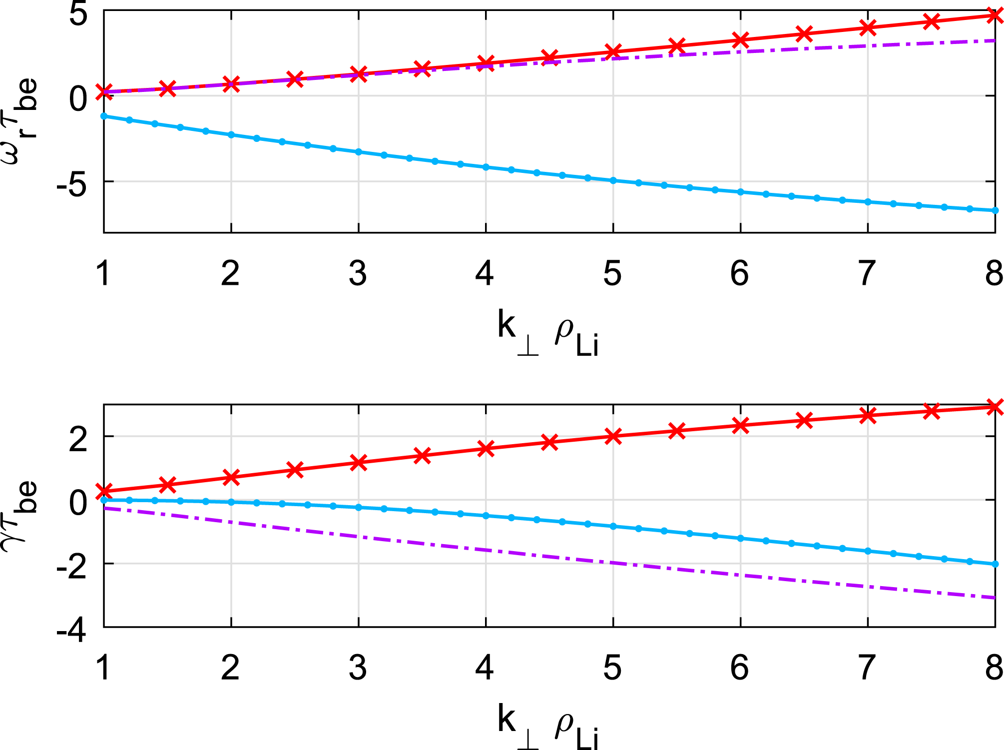
Normalized frequency (a)
 $\unicode[STIX]{x1D714}_{r}\unicode[STIX]{x1D70F}_{be}$
and growth rate (b) as a function of normalized wavenumber
 $k_{\bot }\unicode[STIX]{x1D70C}_{Li}$
, solutions of dispersion relation (3.17) with typical near-Earth plasma sheet parameters:
 $T_{i}=2~\text{keV}$
,
 $T_{e}=500~\text{eV}$
,
 $n_{0}=1~\text{cm}^{-3}$
,
 $c_{A}/V_{i}=2$
and
 $L_{n}=R_{E}/2$
. Only one mode is driven unstable (red line), the two others are damped.

4 Discussion
Equation (3.17) is numerically solved for various density gradient slopes, Alfvén velocities and
 $L$
-shells. Neglecting the thickness of the ionosphere, the farthest mirror point on the field line is always identified with the ground footpoint. Before investigating a parametric study let us consider a representative example of the dispersion relation. The Alfvén velocity is fixed to
 $c_{A}=2V_{i}$
and the magnetic ratio
 $\unicode[STIX]{x1D700}=10^{-3}$
corresponding to an
 $L$
-shell around 8. Figure 2 shows the dispersion curves drawn for the density gradient slope
 $L_{n}=R_{E}/2$
. Top (respectively bottom) panel displays the real part of the normalized frequency
 $\unicode[STIX]{x1D714}_{r}\unicode[STIX]{x1D70F}_{be}$
(respectively the imaginary part
 $\unicode[STIX]{x1D6FE}\unicode[STIX]{x1D70F}_{be}$
or growth rate) as a function of the real wavenumber
 $k_{\bot }\unicode[STIX]{x1D70C}_{Li}$
. Three modes are found to propagate along the
 $y$
-axis. Two of them have a real frequency while the third one has a negative frequency. This simply means that the latter propagates in the negative
 $y$
direction (electron drift). From the sign of the imaginary part one notices that only one propagating mode is unstable with a quite strong growth rate of the order of the bounce frequency. The two others are damped. The unstable mode (red line) propagates in the positive
 $y$
direction (ion drift). To gain a deeper understanding of the nature of the propagating modes, it is useful to introduce the wave impedance normalized to the Alfvén velocity (Onishchenko et al.
Reference Onishchenko, Pokhotelov, Krasnoselskikh and Shatalov2009):
 $$\begin{eqnarray}w.i.=\left|\frac{e_{y}}{b_{\unicode[STIX]{x1D713}}c_{A}}\right|\propto \frac{\unicode[STIX]{x1D719}_{1}}{\unicode[STIX]{x1D6FC}_{1}c_{A}}\end{eqnarray}$$
that can be computed directly in terms of
 $\unicode[STIX]{x1D714}$
and
 $k_{y}$
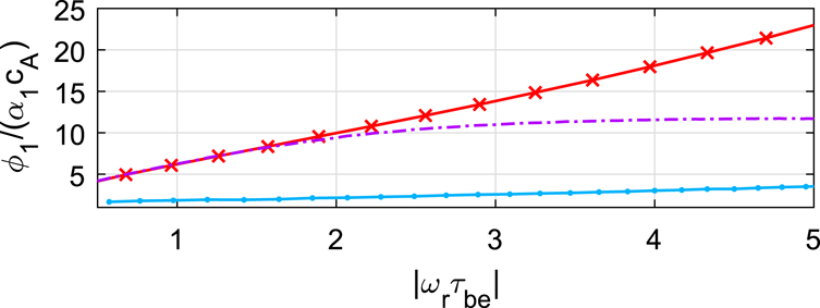
using the dispersion relation (3.17). This parameter should be equal to one for a pure Alfvén wave and is expected to remain close to unity for an Alfvénic mode. Figure 3 shows the normalized wave impedance for the three modes computed on figure 2 using the same pattern. The wave impedance remains less than 5 for the mode propagating in the negative
 $y$
direction (eastward) while it increases strongly with the frequency for the unstable mode. We can conclude that the system supports the propagation of waves with similar polarization and characteristics as Alfvén waves but they are also strongly damped. On the other hand the unstable mode has little to do with Alfvén waves actually. It is more similar to an electrostatic drift wave with a strong wave impedance. This is consistent with the fact that the instability develops principally on the plasma inhomogeneity regardless magnetic perturbations. As we are mostly interested by this instability, the rest of the discussion will focus on this unstable solution only.
Wave impedance
 $\unicode[STIX]{x1D711}_{1}/\unicode[STIX]{x1D6FC}_{1}c_{A}$
as a function of the frequency
 $|\unicode[STIX]{x1D714}_{r}\unicode[STIX]{x1D70F}_{be}|$
for the three modes on figure 2. The eastward propagating damped mode (blue line) is mainly Alfvénic whereas the unstable mode (red line) and the other damped mode are more similar to electrostatic waves (drift waves).

Normalized frequency
 $\unicode[STIX]{x1D714}_{r}\unicode[STIX]{x1D70F}_{be}$
as a function of wavenumber
 $k_{\bot }\unicode[STIX]{x1D70C}_{Li}$
for the electromagnetic drift unstable mode with the near-Earth (at
 $L=8$
) plasma sheet parameters:
 $T_{i}=2~\text{keV}$
,
 $T_{e}=500~\text{eV}$
,
 $n_{0}=1~\text{cm}^{-3}$
,
 $c_{A}/V_{i}=2$
and varying density gradient slope
 $L_{n}$
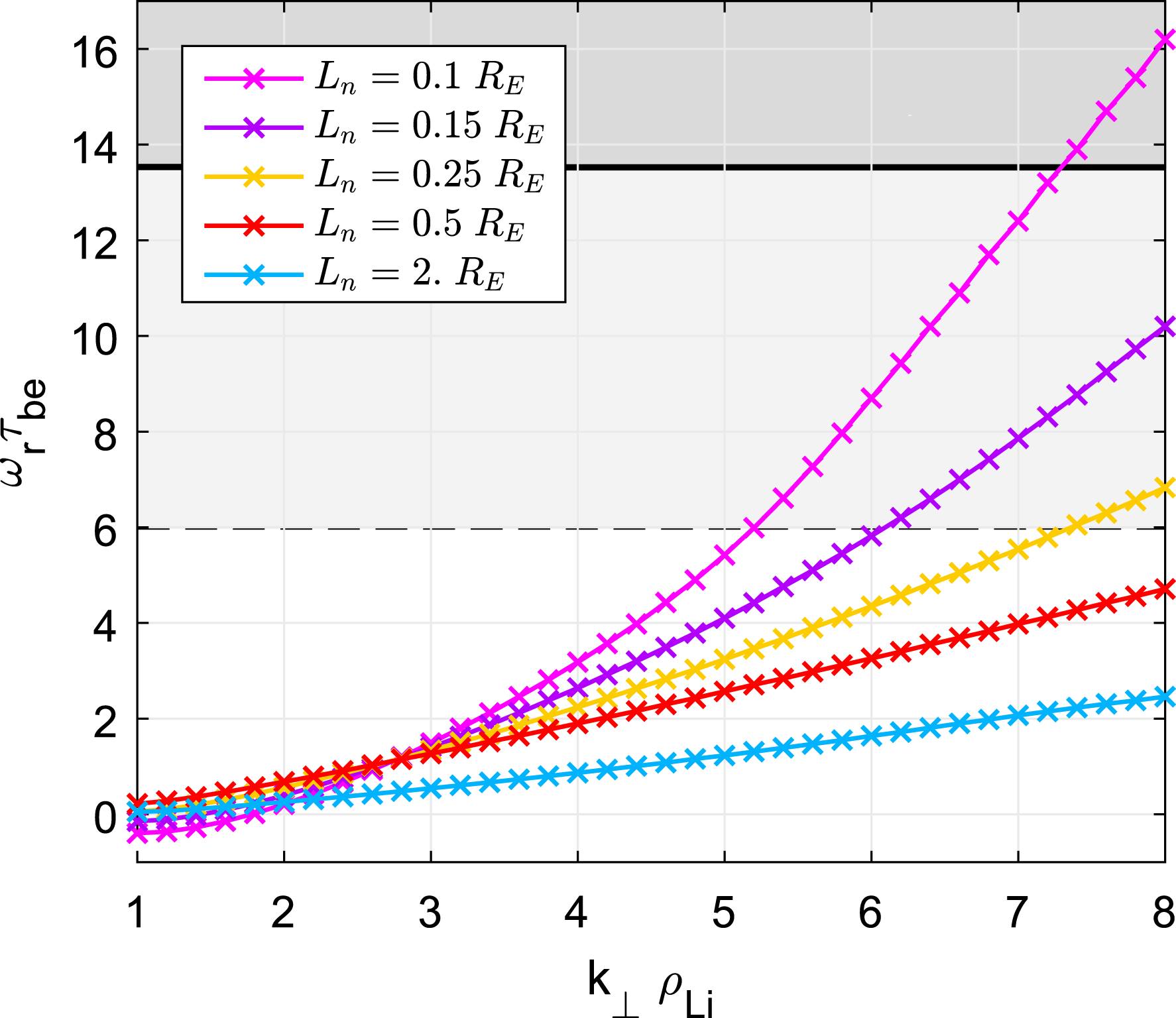
. The frequencies in the shaded region are influenced by the ions’ cyclotron movement, neglected by the theory (
 $\unicode[STIX]{x1D714}\ll \unicode[STIX]{x1D714}_{ci}$
).

The dispersion curves drawn for the unstable wave mode are shown in figures 4 and 5 for several values of the density gradient slope
 $L_{n}$
but with a fixed value of the Alfvén velocity
 $c_{A}=2V_{i}$
and a fixed
 $\unicode[STIX]{x1D700}=10^{-3}$
. To stay within the limits of validity of our model, the frequency should be less than the typical ion cyclotron frequency
 $\unicode[STIX]{x1D714}_{ci}\unicode[STIX]{x1D70F}_{be}\sim 85$
which imposes the wavelength to stay of the order of the ion Larmor radius (
 $k_{\bot }\unicode[STIX]{x1D70C}_{Li}\sim 2\unicode[STIX]{x03C0}$
). For mild density gradient, the real frequency
 $\unicode[STIX]{x1D714}_{r}$
can be approximated by a linear function whose slope depends on the diamagnetic drift velocity
 $u_{i}$
. The phase velocities of the waves are
 $v_{ph}|_{L_{n}=\{0.25,0.5,2\}R_{E}}=\{6.5,4,2.4\}~\text{km}~\text{s}^{-1}$
where the ion drift velocities are
 $u_{i}|_{L_{n}=\{0.25,0.5,2\}R_{E}}=\{22;11;2.7\}~\text{km}~\text{s}^{-1}$
. So the two velocities are of the same order of magnitude, but apparently there is no simple linear relationship between
 $v_{ph}$
and
 $u_{i}$
.
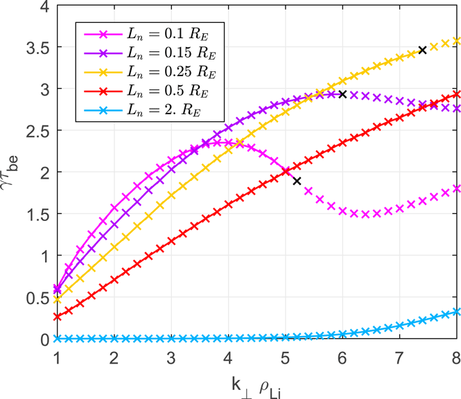
Growth rate
 $\unicode[STIX]{x1D6FE}\unicode[STIX]{x1D70F}_{be}$
as a function of wavenumber
 $k_{\bot }\unicode[STIX]{x1D70C}_{Li}$
for the electromagnetic drift unstable mode with the near-Earth (at
 $L=8$
) plasma sheet parameters:
 $T_{i}=2~\text{keV}$
,
 $T_{e}=500~\text{eV}$
,
 $n_{0}=1~\text{cm}^{-3}$
,
 $c_{A}/V_{i}=2$
and varying density gradient slope
 $L_{n}$
.

Concerning now the growth rate of the instability, we can see from figure 5 that
 $\unicode[STIX]{x1D6FE}$
increases with
 $k_{\bot }$
for all values of
 $L_{n}$
. Actually, if the curves are continued to higher values of
 $k_{\bot }$
, it can be checked that
 $\unicode[STIX]{x1D6FE}$
reaches a maximum and then decreases. But this maximum growth rate is obtained for an irrelevant value of either the wavenumber or the frequency. It is probably due to the simplifications adopted in the model, especially the fact that ion cyclotron effects are not considered, whereas they should play a definitive role in this range of frequencies/wavenumbers.
More interesting is the variation of
 $\unicode[STIX]{x1D6FE}$
with the density gradient scale
 $L_{n}$
. For a very weak diamagnetic drift velocity corresponding to
 $L_{n}$
, above
 $2R_{E}$
the growth rate remains harmless for sensible wavenumbers. In this case the mode grows too slowly to destabilize the current sheet in tens of seconds and we may conclude that the plasma sheet is stable. As the density gradient is steepening the growth rate becomes of the same order as the real frequency, revealing a very fast instability. The maximum growth rate is obtained for
 $L_{n}=0.25R_{E}$
corresponding to a normalized diamagnetic drift velocity
 $u_{d}\sim 0.02$
. For a higher drift velocity we observe a drop in the maximum growth rate, which corresponds to much smaller wavenumber. For instance, at a wavelength of the order of one Larmor radius (
 $k_{\bot }\unicode[STIX]{x1D70C}_{Li}=2\unicode[STIX]{x03C0}$
), the e-folding time
 $2\unicode[STIX]{x03C0}/\unicode[STIX]{x1D6FE}$
of the instability is approximately 25 min for
 $L_{n}=2.5R_{E}$
, a too long time to really destabilize the magnetic structure, but it drops to 30 s for
 $L_{n}=0.25R_{E}$
.
Comparison with the pure electrostatic drift instability (Fruit et al.
Reference Fruit, Louarn and Tur2017) shows that growth rates of the electromagnetic drift modes are an order of magnitude lower than that of electrostatic drift waves with the same diamagnetic drift velocity. For example, for wavenumber
 ${\sim}0.026~\text{km}^{-1}$
and the diamagnetic drift velocity
 $u_{i}\sim 11~\text{km}~\text{s}^{-1}$
(
 $u_{d}\sim 0.02$
), corresponding to the density gradient slope
 $L_{n}=0.5R_{E}$
, the amplitude growth rate of the electrostatic drift waves is
 ${\sim}0.13~\text{s}^{-1}$
and that of the electromagnetic drift wave is
 ${\sim}0.05~\text{s}^{-1}$
. In other words, the perturbation in the parallel current produces a kind of stabilization effect on the drift instability.
Let us now investigate the influence of parameters such as the Alfvén velocity
 $c_{A}$
or the stretching constant
 $\unicode[STIX]{x1D700}=B_{0}/B_{1}$
on the boundary between stable and unstable wave modes. We may choose this boundary at a normalized growth rate of
 $0.5$
. With a typical bounce period of 14 s (see table 1) modes with a growth rate less than
 $\unicode[STIX]{x1D6FE}\unicode[STIX]{x1D70F}_{be}=0.5$
have an e-folding time longer than 3 minutes and we may consider those as stable as they do not contribute to the rapid destabilization of the plasma sheet observed during a usual substorm onset.
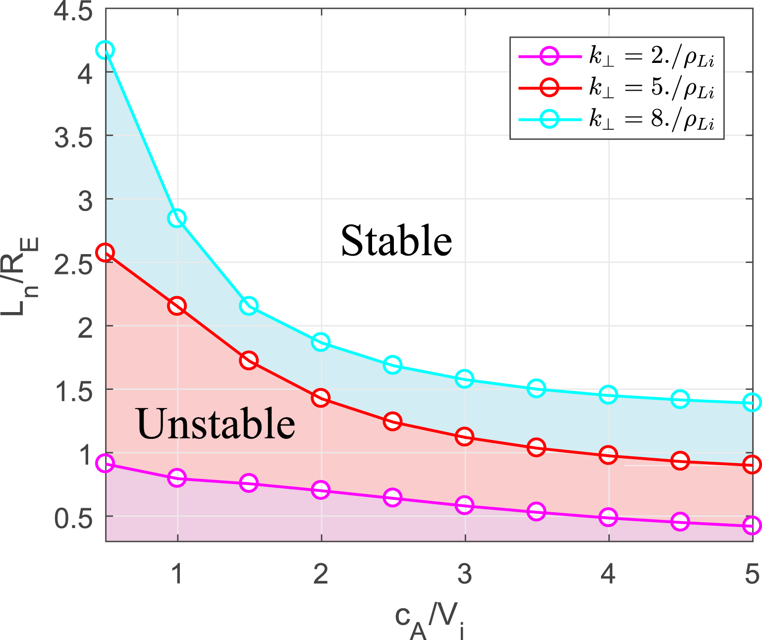
Figure 6 displays in the
 $(L_{n},c_{A})$
plane the instability threshold
 $\unicode[STIX]{x1D6FE}\unicode[STIX]{x1D70F}_{be}=0.5$
for a few representative wavenumbers and
 $L=8$
. The shaded area corresponds to the unstable mode. This means for instance that for the Alfvén velocity
 $c_{A}=2V_{i}$
, the electromagnetic drift mode becomes potentially unstable for the equilibrium of the sheet if the density gradient scale is smaller than
 $1.87R_{E}$
for a wavelength of 0.75 times the ion Larmor radius (
 $k_{\bot }\unicode[STIX]{x1D70C}_{Li}=8$
) but it should be smaller than
 $0.7R_{E}$
for a larger wavelength, of the order of 3 Larmor radii (
 $k_{\bot }\unicode[STIX]{x1D70C}_{Li}=2$
). Thus, perturbations with smaller perpendicular wavelengths are more likely to be driven unstable. The ratio of the Alfvén velocity to the ion thermal speed also modifies the position of the instability threshold. The plasma sheet tends to be harder to destabilize when the
 $c_{A}/V_{i}$
is high. On the contrary, for a low ratio
 $c_{A}/V_{i}<1$
, i.e. with denser and hotter ions, a much milder density gradient is sufficient to excite the electromagnetic drift instability.
The density gradient slope
 $L_{n}$
as a function of the Alfvén speed
 $c_{A}$
with
 $\unicode[STIX]{x1D6FE}\unicode[STIX]{x1D70F}_{be}=0.05$
,
 $\unicode[STIX]{x1D700}=1.1\times 10^{-3}$
on
 $L=8$
and varying wavenumber
 $k_{\bot }$
. The plasma parameters in the shaded region correspond to the unstable mode.

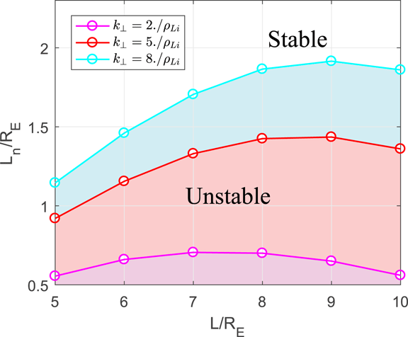
Figure 7 displays the same instability threshold
 $\unicode[STIX]{x1D6FE}\unicode[STIX]{x1D70F}_{be}=0.5$
but in the
 $(L_{n},L)$
plane for
 $c_{A}/V_{i}=2$
. Changing the
 $L$
-shell acts principally on the stretching parameter
 $\unicode[STIX]{x1D716}=B_{0}/B_{1}$
given the fact that
 $B_{1}$
is the value of the magnetic field at the ground. It is noticeable that the instability threshold adopts a parabolic profile versus
 $L$
with a maximum localized in the near-Earth region of the magnetotail. The maximum of the parabola corresponds to the optimal magnetic shell on which the probability of instability onset at low density gradient is higher. Modes with wavenumber
 $k_{\bot }\unicode[STIX]{x1D70C}_{Li}=8$
are likely to become unstable at
 $L=9$
whereas modes with smaller wavenumber
 $k_{\bot }\unicode[STIX]{x1D70C}_{Li}=2$
are driven unstable with a steeper density gradient at a closer shell (
 $L=7$
) to the Earth. Obviously this result also depends on the Alfvèn velocity, but one can check that the position of the maximum is only slightly shifted away from the Earth when
 $c_{A}/V_{i}$
is increased. An interesting outcome of this parametric analysis is to show that a progressive increase of the density gradient leads to an instability developing first at
 $L\sim 7{-}9$
which is consistent with observations of near-Earth substorm onset (Roux et al.
Reference Roux, Perraut, Robert, Morane, Pedersen, Korth, Kremser, Aparicio, Rodgers and Pellinen1991).
The density gradient slope
 $L_{n}$
as a function of the magnetic
 $L$
-shell with
 $\unicode[STIX]{x1D6FE}\unicode[STIX]{x1D70F}_{be}=0.05$
,
 $c_{A}=2V_{i}$
and varying wavenumber
 $k_{\bot }\unicode[STIX]{x1D70C}_{Li}$
.

5 Conclusion
This theoretical study aims to investigate the resonant interaction between electromagnetic fluctuations with trapped bouncing electrons in the near-Earth tail of the magnetosphere (
 $8<L<12$
), characterized by a high density gradient
 $\unicode[STIX]{x1D735}n\Vert \boldsymbol{e}_{x}$
and a small field line curvature. Assuming a low plasma
 $\unicode[STIX]{x1D6FD}\ll 1$
, only parallel currents and torsional perturbations are considered in this first study. Starting with a particle distribution function respecting the invariance along the
 $y$
-axis, the Vlasov equation is integrated along the unperturbed particle trajectories, including cyclotron and bounce motions. A Fourier expansion has been assumed first to model the spatial structure of the electromagnetic potential and second to decompose the bounce motion. Only the first term of these expansions has been conserved in this first analysis but generalizations with other harmonics are possible. Ion cyclotron effects have also been neglected in this first approach of the problem and could be possibly included in future investigations. Taking these restrictions into account, integration over cyclotron motion and electron bounce oscillations allows us to write perturbed distribution functions as a linear combination of potentials. The dispersion relation is then obtained analytically via the plasma quasi-neutrality condition and Ampere’s law for the parallel current.
Unstable electromagnetic drift modes have been found to propagate in the positive
 $y$
-direction, i.e. in the same direction as the ion drift (westwards) with a phase velocity of the order of the ion drift velocity. These modes oscillate at about the thermal electron bounce period
 $({\sim}15~\text{s})$
with a wavelength of the order of the ion Larmor radius (80 km). The growth rate strongly depends on the slope of the density gradient. For typical gradient scales larger than
 $2R_{E}$
, drift effects are too weak to produce a fast growing instability, as the e-folding time of the perturbations is longer than a few minutes. The mode becomes potentially unstable with e-folding time less than 1 minute if the density gradient steepens with scale less than
 $0.5{-}1R_{E}$
. This instability threshold depends on the Alfvén velocity at the equatorial plane and on the magnetic
 $L$
-shell. It has been showed that a larger Alfvèn velocity tends to stabilize the plasma sheet and a much sharp density gradient is required to get large growth rate. On the other hand, the instability threshold presents a maximum along the
 $L$
-shell meaning that the electromagnetic drift instability may develop more easily on a particular magnetic shell depending on its perpendicular wavelength.
Some authors have nevertheless reported observations of aurora arcs with a beading structure (Kalmoni et al.
Reference Kalmoni, Rae, Watt, Murphy, Forsyth and Owen2015; Lui Reference Lui2016; Miyashita et al.
Reference Miyashita, Angelopoulos, Fukui and Machida2018) that could be a visual manifestation of this drift-Alfvén instability. From the all-sky images (ASI) of auroral arcs it is found that the growth rate of the instability covers the range
 $0.02{-}0.3~\text{s}^{-1}$
. With a typical bounce period of 15 s, this corresponds to normalized growth rate between 0.3 and 4.5, which matches the growth rate found in figure 5 with a density gradient scale of the order of
 $0.5R_{E}$
. A precise comparison between observations of auroral arcs and the theoretical results of our model remains to be carried out. But the output of this new kinetic model may help substantially to understand the triggering processes of instability in the near-Earth region at the origin of some aurora arcs. The present treatment is still somewhat limited by several assumptions that we plan to reconsider in the near future. First cyclotron effects may be important to include in order to regularize the behaviour of the instability at larger wavenumber and higher frequencies. Second, a full electromagnetic theory that includes the curvature effects is still needed to model a similar type of electromagnetic bounce instability in a stretched magnetotail configuration. One of the mechanisms that is widely believed to play an important role in triggering substorms in the near-Earth magnetotail is the ballooning instability (Roux et al.
Reference Roux, Perraut, Robert, Morane, Pedersen, Korth, Kremser, Aparicio, Rodgers and Pellinen1991). It is however inappropriate to compare the present study to known kinetic theories of ballooning modes (Cheng Reference Cheng1982) since ballooning instability implies the effect of field line curvature (and moderate
 $\unicode[STIX]{x1D6FD}$
) that we have not taken into account here. The relationship between the full electromagnetic drift instability with the kinetic ballooning instability would be nevertheless a very interesting issue to investigate in the future.
Appendix A. Curvilinear coordinate system
The natural field-aligned coordinates system
 $(\unicode[STIX]{x1D713},y,\unicode[STIX]{x1D712})$
is defined by
 $$\begin{eqnarray}\boldsymbol{e}_{\unicode[STIX]{x1D713}}=[\boldsymbol{e}_{y}\times \boldsymbol{e}_{\unicode[STIX]{x1D712}}],\quad \boldsymbol{e}_{y}=\frac{\boldsymbol{J}_{eq}}{J_{eq}},\quad \boldsymbol{e}_{\unicode[STIX]{x1D712}}=\frac{\boldsymbol{B}_{eq}}{B_{eq}},\end{eqnarray}$$
where
 $B_{eq}(\unicode[STIX]{x1D712},\unicode[STIX]{x1D713})$
and
 $J_{eq}(y)$
are the magnetic field and electric current at equilibrium. According to Tur et al. (Reference Tur, Fruit, Louarn and Yanovsky2014), the scale factors in the curvilinear system are
 $$\begin{eqnarray}h_{\unicode[STIX]{x1D713}}=\frac{1}{B_{eq}},\quad h_{y}=1,\quad h_{\unicode[STIX]{x1D712}}=JB_{eq}=\frac{1}{B_{eq}}\exp \left[-\unicode[STIX]{x1D707}_{0}\int \frac{J_{eq}}{B_{eq}^{2}}\,\text{d}\unicode[STIX]{x1D713}\right],\end{eqnarray}$$
where
 $J$
denotes the Jacobian of the coordinate transformation. The elementary length along the field line is given by
 $$\begin{eqnarray}\text{d}\ell =h_{\unicode[STIX]{x1D712}}\,\text{d}\unicode[STIX]{x1D712}.\end{eqnarray}$$
The nabla operator writes
 $$\begin{eqnarray}\unicode[STIX]{x1D735}=B_{eq}\frac{\unicode[STIX]{x2202}}{\unicode[STIX]{x2202}\unicode[STIX]{x1D713}}\boldsymbol{e}_{\unicode[STIX]{x1D713}}+\frac{\unicode[STIX]{x2202}}{\unicode[STIX]{x2202}y}\boldsymbol{e}_{y}+\frac{1}{JB_{eq}}\frac{\unicode[STIX]{x2202}}{\unicode[STIX]{x2202}\unicode[STIX]{x1D712}}\boldsymbol{e}_{\unicode[STIX]{x1D712}}.\end{eqnarray}$$
The resolution of the parallel Ampere law requires us to compute the parallel component of the Laplacian of
 $\boldsymbol{a}_{1}$
using the algebraic formula
 $\unicode[STIX]{x0394}\boldsymbol{a}=\unicode[STIX]{x1D735}(\unicode[STIX]{x1D735}\boldsymbol{\cdot }\boldsymbol{a})-[\unicode[STIX]{x1D735}\times [\unicode[STIX]{x1D735}\times \boldsymbol{a}]]$
(see also (38) of Tur et al. (Reference Tur, Fruit, Louarn and Yanovsky2014))
 $$\begin{eqnarray}[\unicode[STIX]{x0394}\boldsymbol{a}_{1}]_{\Vert }=-k_{\bot }^{2}\tilde{a}_{\Vert }+\frac{\text{d}^{2}\tilde{a}_{\Vert }}{\text{d}\ell ^{2}}-\frac{\text{d}}{\text{d}\ell }\left(\frac{\text{d}\ln B_{eq}}{\text{d}\ell }\tilde{a}_{\Vert }\right).\end{eqnarray}$$
Taking the Fourier component along the field line to get
 $j_{\Vert }$
also given by (2.33), Ampere’s law for the parallel current in the curvilinear system is
 $$\begin{eqnarray}\unicode[STIX]{x1D707}_{0}j_{\Vert }=\left[k_{\bot }^{2}+\frac{\unicode[STIX]{x03C0}^{2}}{\ell _{0}^{2}}(1-\unicode[STIX]{x1D6FD}_{0})\right]\unicode[STIX]{x1D6FC}_{1},\end{eqnarray}$$
with coefficient
 $\unicode[STIX]{x1D6FD}_{0}=-(2/\unicode[STIX]{x03C0})\int _{0}^{\ell _{0}}(\text{d}\ln B_{eq})/(\text{d}\ell )\sin (\unicode[STIX]{x03C0}(\ell /\ell _{0}))\cos (\unicode[STIX]{x03C0}(\ell /\ell _{0}))\,\text{d}\ell$
of the order of unity. This last expression for the Laplacian may be simplified in our analysis since the wavelength is assumed to be of the order of the ion Larmor radius and
 $k_{\bot }\sim \unicode[STIX]{x03C0}/\unicode[STIX]{x1D70C}_{Li}\sim 1200\unicode[STIX]{x03C0}/\ell _{0}$
given the parameters in table 1, thus
 $$\begin{eqnarray}\unicode[STIX]{x1D707}_{0}j_{\Vert }=k_{\bot }^{2}\unicode[STIX]{x1D6FC}_{1}.\end{eqnarray}$$
Appendix B. Expressions for some functions appearing in (3.8)–(3.11)
Introducing the variable
 $\unicode[STIX]{x1D701}$
written in the dimensionless quantities
 $x$
and
 $\unicode[STIX]{x1D700}=B_{0}/B_{1}$
:
 $$\begin{eqnarray}\unicode[STIX]{x1D701}=\frac{\unicode[STIX]{x03C0}}{2}\sqrt{\frac{E-\unicode[STIX]{x1D707}B_{0}}{\unicode[STIX]{x1D707}B_{1}}}=\frac{\unicode[STIX]{x03C0}}{2}\sqrt{\frac{\unicode[STIX]{x03C0}^{2}}{x^{2}}-\unicode[STIX]{x1D700}},\end{eqnarray}$$
the functions
 $\unicode[STIX]{x1D6E4}_{0,\ldots ,4}(x)$
in the integrals (3.8)–(3.11) write
 $$\begin{eqnarray}\displaystyle & \displaystyle \unicode[STIX]{x1D6E4}_{0}=\left(\frac{1}{2}J_{0}^{2}(\unicode[STIX]{x1D701})+J_{2}^{2}(\unicode[STIX]{x1D701})\right)\left[\frac{\unicode[STIX]{x03C0}^{2}}{x^{2}}+\unicode[STIX]{x1D700}\right]-J_{0}(\unicode[STIX]{x1D701})J_{2}(\unicode[STIX]{x1D701})\left[\frac{\unicode[STIX]{x03C0}^{2}}{x^{2}}-\unicode[STIX]{x1D700}\right] & \displaystyle\end{eqnarray}$$
 $$\begin{eqnarray}\displaystyle & \displaystyle \unicode[STIX]{x1D6E4}_{1}=-J_{2}^{2}(\unicode[STIX]{x1D701})\left[\frac{\unicode[STIX]{x03C0}^{2}}{x^{2}}+\unicode[STIX]{x1D700}\right]+\frac{1}{2}J_{0}(\unicode[STIX]{x1D701})J_{2}(\unicode[STIX]{x1D701})\left[\frac{\unicode[STIX]{x03C0}^{2}}{x^{2}}-\unicode[STIX]{x1D700}\right] & \displaystyle\end{eqnarray}$$
 $$\begin{eqnarray}\displaystyle & \displaystyle \unicode[STIX]{x1D6E4}_{2}=J_{1}(\unicode[STIX]{x1D701})J_{2}(\unicode[STIX]{x1D701})\left[\frac{\unicode[STIX]{x03C0}^{2}}{x^{2}}+\unicode[STIX]{x1D700}\right]-\frac{1}{2}J_{0}(\unicode[STIX]{x1D701})J_{1}(\unicode[STIX]{x1D701})\left[\frac{\unicode[STIX]{x03C0}^{2}}{x^{2}}-\unicode[STIX]{x1D700}\right] & \displaystyle\end{eqnarray}$$
 $$\begin{eqnarray}\displaystyle & \displaystyle \unicode[STIX]{x1D6E4}_{3}=\frac{1}{2}J_{1}(\unicode[STIX]{x1D701})J_{2}(\unicode[STIX]{x1D701})\left[\frac{\unicode[STIX]{x03C0}^{2}}{x^{2}}+\unicode[STIX]{x1D700}\right] & \displaystyle\end{eqnarray}$$
 $$\begin{eqnarray}\displaystyle & \displaystyle \unicode[STIX]{x1D6E4}_{4}=\frac{1}{2}J_{1}^{2}(\unicode[STIX]{x1D701})\left[\frac{\unicode[STIX]{x03C0}^{2}}{x^{2}}+\unicode[STIX]{x1D700}\right]. & \displaystyle\end{eqnarray}$$