1 Introduction
Energy transfer is a fundamental process in turbulence. It is closely related to the multi-scale feature and spatial inhomogeneity of turbulent flows. In the description of the energy cascade process (Richardson Reference Richardson1922), the successive energy transfer from large to small scales was exhibited. Under the assumption of homogeneity and isotropy, the asymptotic statistics of small-scale motions at very high Reynolds numbers were obtained by Kolmogorov (Reference Kolmogorov1941a), e.g. the scaling of the moments of velocity increments. In addition, the energy cascade among different length scales is described by the Kolmogorov equation (Kolmogorov Reference Kolmogorov1941b), where the unidirectional energy flux from large to small scales is related to the averaged dissipation rate. After Kolmogorov’s pioneering work, many efforts have been devoted to the study of the multi-scale behaviour of turbulent flows (e.g. Kraichnan Reference Kraichnan1971; Meneveau & Katz Reference Meneveau and Katz2000; Vassilicos Reference Vassilicos2015; Dubrulle Reference Dubrulle2019).
Compared with homogeneous turbulence, the energy transfer process becomes more complex in wall-bounded turbulent flows due to spatial inhomogeneity. Starting from the two-point correlation transport equation, Lumley (Reference Lumley1964) analysed the spectral energy budget in wall-bounded turbulence and deduced that inverse energy transfer occurs due to the energy and pressure fluxes in the wall-normal direction. In the past few decades, direct numerical simulation (DNS) has provided evidence for the existence of the inverse energy cascade. Domaradzki et al. (Reference Domaradzki, Liu, Härtel and Kleiser1994) observed inverse energy transfer and showed the scale locality of the energy cascade in low-Reynolds-number wall-bounded turbulent flows. Using DNS data up to  $Re_{\unicode[STIX]{x1D70F}}=5200$, where
 $Re_{\unicode[STIX]{x1D70F}}$ is the friction Reynolds number based on the friction velocity and channel half-width, Lee & Moser (Reference Lee and Moser2015) performed a spectral analysis of the terms in the transport equation of the two-point velocity correlation and also observed inverse energy transfer. Cho, Hwang & Choi (Reference Cho, Hwang and Choi2018) visualized the triadic interactions involved in the turbulent energy transport in a turbulent channel flow of
 $Re_{\unicode[STIX]{x1D70F}}=1700$ to illustrate the existence of energy transfer from small- to large-scale motions, but the classical energy cascade was found still to be the dominant transfer mechanism. Recently, Mizuno (Reference Mizuno2016) revealed the scale dependence of spatial turbulent kinetic energy transport in a channel flow up to
 $Re_{\unicode[STIX]{x1D70F}}=1000$. The downward energy flux at large scales was found to be responsible for the Reynolds number dependence of turbulence intensity. Later, Lee & Moser (Reference Lee and Moser2019) observed the same phenomenon from their
 $Re_{\unicode[STIX]{x1D70F}}=5200$ DNS dataset, and further studied the interaction between the near-wall dynamics and the outer-layer turbulence dominated by very-large-scale motions. In the above studies, the inter-scale energy transfer in the wall-parallel directions and the spatial energy transport in the wall-normal direction were the main concern, and the wall-normal scales were not considered.
While in the studies mentioned above spectral analyses were applied to the homogeneous wall-parallel plane to extract the scale dependence of energy transfer, the statistics in physical space may provide further insight. Hill (Reference Hill2002) derived the balance equation for the second-order structure function in anisotropic turbulence to establish the relation between the second- and third-order moments, which can be physically interpreted as the scale energy and the scale-energy flux, respectively. Using the generalized Kolmogorov equation, Marati, Casciola & Piva (Reference Marati, Casciola and Piva2004) evaluated the scale-by-scale balance in different regions of a channel flow. Along this line, Cimarelli, De Angelis & Casciola (Reference Cimarelli, De Angelis and Casciola2013) observed an ascending spiral-like energy transfer path in the combined space of wall-parallel scales and wall-normal distance. They found that the inverse energy cascade plays a key role in the formation of the very long streaks of velocity fluctuations. Later, the generalized Kolmogorov equation was further studied by Cimarelli et al. (Reference Cimarelli, De Angelis, Jiménez and Casciola2016) in the reduced space of wall-normal and spanwise scales and wall-normal distance.
While considerable progress has been made in understanding the energy transfer in canonical wall-bounded turbulent flows as reviewed above, there has been much less work on the energy transfer process in wall-bounded turbulence with a travelling wavy boundary, for instance, in the framework of wind–wave interaction (Sullivan & McWilliams Reference Sullivan and McWilliams2010). Surface waves carry a new energy source and multi-scale waving motions, which may significantly affect the energy transfer process in the overlying turbulent flow. In the early years, several theoretical models, e.g. the resonance mechanism (Phillips Reference Phillips1957) and the critical layer theory (Miles Reference Miles1957), were proposed to explain the wind–wave generation process and to predict the wave growth rate. Later, Belcher & Hunt (Reference Belcher and Hunt1993) and Cohen & Belcher (Reference Cohen and Belcher1999) performed analyses of the non-separated sheltering phenomenon of slow- and fast-moving waves, respectively, based on the rapid distortion theory, to explain the momentum transfer between airflow and surface waves. In recent years, laboratory measurements and field observations have provided valuable flow-field data, which yield important insights into the physical process of wind–wave interaction. For example, using laboratory measurements, Buckley & Veron (Reference Buckley and Veron2016, Reference Buckley and Veron2019) obtained the instantaneous and phase-averaged velocity fields of the airflow above surface waves for different wind–wave conditions. Meanwhile, field observations in open sea provide data of the flow field at the air–sea interface over a wide range of scales. In Black et al. (Reference Black, D’Asaro, Drennan, French, Niiler, Sanford, Terrill, Walsh and Zhang2007), air–sea exchange measurements were conducted to improve the parameterization of weather forecast models, such as hurricane intensity. In Hristov, Miller & Friehe (Reference Hristov, Miller and Friehe2003) and Grare, Lenain & Melville (Reference Grare, Lenain and Melville2013), evidences of the Miles critical layer theory were obtained from field observations.
With the rapid increase in computing power and advances in algorithm development, numerical simulation has become a useful tool for studying wind–wave interactions. Based on the DNS data of turbulent airflows over idealized water waves, the waves were found to have significant influence on the mean flow, vertical momentum transfer, form drag, coherent structures, scalar transport and very-large-scale motions in the air (Sullivan, McWilliams & Moeng Reference Sullivan, McWilliams and Moeng2000; Kihara et al. Reference Kihara, Hanazaki, Mizuya and Ueda2007; Yang & Shen Reference Yang and Shen2009; Druzhinin, Troitskaya & Zilitinkevich Reference Druzhinin, Troitskaya and Zilitinkevich2012; Yang & Shen Reference Yang and Shen2017; Zhang, Huang & Xu Reference Zhang, Huang and Xu2019), and the effects depend on the water wave properties, including the wave steepness, wave age, wave nonlinearity and wind-induced surface drift (e.g. Yang & Shen Reference Yang and Shen2010). In addition to the monochromatic travelling wave as an idealized case, the broadband wave field containing multi-scale wave motions is a more realistic representation of the sea condition. However, there are fewer studies of the interaction between broadband waves and wind turbulence due to the additional complexity associated with an irregular wave system over a wide range of scales. Liu et al. (Reference Liu, Yang, Guo and Shen2010) adopted the high-order spectral (HOS) method (Dommermuth & Yue Reference Dommermuth and Yue1987) for simulating the dynamic evolution of broadband nonlinear waves under wind forcing and quantified the wave growth rate for different wave components. They found that the wave growth rate can be approximated by the corresponding monochromatic components for long waves, while stochastic modelling is called for in the case of short waves. Sullivan, McWilliams & Patton (Reference Sullivan, McWilliams and Patton2014) performed large-eddy simulation of wind turbulence over a broadband spectrum of moving waves, and observed that the wind profile deviates from the Monin–Obukhov similarity theory under non-equilibrium wind–wave conditions. Very recently, Hao & Shen (Reference Hao and Shen2019) studied wind turbulence over broadband waves with a focus on the long-term evolution of the nonlinear wave field. As an application, Yang, Meneveau & Shen (Reference Yang, Meneveau and Shen2014) investigated an offshore wind farm under different wind–sea conditions, and observed that the fully developed wind–sea condition induces less resistance to the wind as compared with the fetch-limited wind–sea condition, and has more wind energy available to harvest.
The aim of the present work is to investigate the turbulent energy transfer process under the impact of broadband waves. Because the surface waves can affect the turbulent coherent structures and momentum transfer, the scale and spatial characteristics of the energy transfer process may differ appreciably from those in canonical wall-bounded turbulent flows. For this purpose, the HOS method is adopted to capture the nonlinear multi-scale water wave motions. The HOS method has been validated extensively in previous studies (Dommermuth & Yue Reference Dommermuth and Yue1987; Tanaka Reference Tanaka2001; Xiao et al. Reference Xiao, Liu, Wu and Yue2013). The overlying three-dimensional, instantaneous airflow data are obtained using DNS, which is coupled to the wave simulation through the air–sea boundary conditions following Yang & Shen (Reference Yang and Shen2010, Reference Yang and Shen2011). From the DNS data, unique features of the airflow over both slow and fast wave fields are identified from the instantaneous turbulent flow field and the turbulence statistics, such as the turbulent energy spectrum. Furthermore, spectral analysis of the two-point correlation transport equation in curvilinear coordinates is performed to reveal the energy transfer process in the flow over broadband waves. Here, the focus of study is on the surface wave effects on the energy transfer process among different length scales in spectral space and different vertical locations in physical space, which is important for improving the parameterization of surface wave effects on marine atmospheric surface layers (Black et al. Reference Black, D’Asaro, Drennan, French, Niiler, Sanford, Terrill, Walsh and Zhang2007; Edson et al. Reference Edson, Crawford, Crescenti, Farrar, Frew, Gerbi, Helmis, Hristov, Khelif and Jessup2007; Chen et al. Reference Chen, Zhao, Donelan and Tolman2013; Breivik et al. Reference Breivik, Mogensen, Bidlot, Balmaseda and Janssen2015). The rest of this paper is organized as follows. The problem formulation and numerical method are briefly introduced in § 2. The instantaneous flow field, energy spectrum and detailed analyses of the energy transfer process are presented in § 3. Finally, conclusions are drawn in § 4.
2 Problem formulation and numerical method
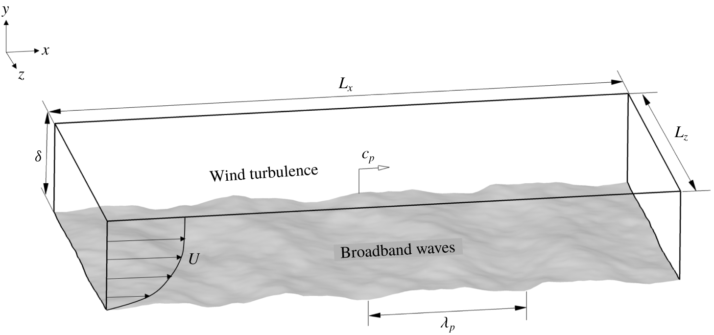
The problem under consideration is a fully developed three-dimensional turbulent flow over water waves. As shown in figure 1, the fluid motion is defined in the Cartesian coordinates  $(x_{1},x_{2},x_{3})$, or equivalently
 $(x,y,z)$, where
 $x,y$ and
 $z$ denote the streamwise, vertical and spanwise directions, respectively. The water wave motions are assumed to be irrotational with periodic boundary conditions. The initial wave field is prescribed based on a broadband wave spectrum. At the peak (denoted by subscript ‘
 $p$’) wavenumber
 $(k_{p})$ of the wave spectrum, the corresponding wave parameters depicted in figure 1 are the wavelength
 $(\unicode[STIX]{x1D706}_{p})$ and the phase speed
 $(c_{p})$.
2.1 Governing equations
The governing equations for the turbulent flow are the dimensionless incompressible Navier–Stokes equations and the continuity equation:
 $$\begin{eqnarray}\displaystyle & \displaystyle \frac{\unicode[STIX]{x2202}\boldsymbol{u}}{\unicode[STIX]{x2202}t}+\boldsymbol{u}\boldsymbol{\cdot }\unicode[STIX]{x1D735}\boldsymbol{u}=-\unicode[STIX]{x1D735}p+\frac{1}{Re}\unicode[STIX]{x1D6FB}^{2}\boldsymbol{u}, & \displaystyle\end{eqnarray}$$
 $$\begin{eqnarray}\displaystyle & \displaystyle \unicode[STIX]{x1D735}\boldsymbol{\cdot }\boldsymbol{u}=0, & \displaystyle\end{eqnarray}$$
where  $\boldsymbol{u}=(u_{1},u_{2},u_{3})$ or equivalently
 $(u,v,w)$ denotes the flow velocity vector,
 $p$ is the dynamic pressure normalized by
 $\unicode[STIX]{x1D70C}U_{m}^{2}$ and
 $Re=U_{m}\unicode[STIX]{x1D6FF}/\unicode[STIX]{x1D708}$ is the bulk Reynolds number, with
 $U_{m}$ being the bulk velocity,
 $\unicode[STIX]{x1D708}$ the kinematic viscosity and
 $\unicode[STIX]{x1D6FF}$ the channel half-width.
The DNS of the turbulent flow is carried out using the pseudo-spectral method based on a boundary-fitted mesh (Ge, Xu & Cui Reference Ge, Xu and Cui2010; Zhang et al. Reference Zhang, Huang and Xu2019). For this purpose, with a strategy similar to that applied in previous studies (Choi, Moin & Kim Reference Choi, Moin and Kim1993; Sullivan et al. Reference Sullivan, McWilliams and Moeng2000; Hara & Sullivan Reference Hara and Sullivan2015; Husain et al. Reference Husain, Hara, Buckley, Yousefi, Veron and Sullivan2019), the governing (2.1) and (2.2) are transformed into the computational domain by introducing an algebraic mapping:
 $$\begin{eqnarray}t=\unicode[STIX]{x1D70F},\quad x_{1}=\unicode[STIX]{x1D709}_{1},\quad x_{2}=\unicode[STIX]{x1D709}_{2}(1-\unicode[STIX]{x1D702}/\unicode[STIX]{x1D6FF})+\unicode[STIX]{x1D702},\quad x_{3}=\unicode[STIX]{x1D709}_{3},\end{eqnarray}$$
where  $\unicode[STIX]{x1D709}_{1}$,
 $\unicode[STIX]{x1D709}_{2}$,
 $\unicode[STIX]{x1D709}_{3}$ and
 $\unicode[STIX]{x1D70F}$ are the space and time coordinates in the computational domain and
 $\unicode[STIX]{x1D702}$ is the wave surface elevation. Then the governing equations (2.1) and (2.2) are rewritten as follows (Kang & Choi Reference Kang and Choi2000):
 $$\begin{eqnarray}\displaystyle & \displaystyle \frac{\unicode[STIX]{x2202}u_{i}}{\unicode[STIX]{x2202}\unicode[STIX]{x1D70F}}=-\frac{\unicode[STIX]{x2202}u_{i}u_{j}}{\unicode[STIX]{x2202}\unicode[STIX]{x1D709}_{j}}-\unicode[STIX]{x1D719}_{j}\frac{\unicode[STIX]{x2202}u_{i}u_{j}}{\unicode[STIX]{x2202}\unicode[STIX]{x1D709}_{2}}-\frac{\unicode[STIX]{x2202}p}{\unicode[STIX]{x2202}\unicode[STIX]{x1D709}_{i}}+\frac{1}{Re}\frac{\unicode[STIX]{x2202}^{2}u_{i}}{\unicode[STIX]{x2202}\unicode[STIX]{x1D709}_{j}\unicode[STIX]{x2202}\unicode[STIX]{x1D709}_{j}}-\unicode[STIX]{x1D719}_{t}\frac{\unicode[STIX]{x2202}u_{i}}{\unicode[STIX]{x2202}\unicode[STIX]{x1D709}_{2}}-\unicode[STIX]{x1D719}_{i}\frac{\unicode[STIX]{x2202}p}{\unicode[STIX]{x2202}\unicode[STIX]{x1D709}_{2}}+\frac{1}{Re}S(u_{i}), & \displaystyle\end{eqnarray}$$
 $$\begin{eqnarray}\displaystyle & \displaystyle \frac{\unicode[STIX]{x2202}u_{i}}{\unicode[STIX]{x2202}\unicode[STIX]{x1D709}_{i}}=-\unicode[STIX]{x1D719}_{j}\frac{\unicode[STIX]{x2202}u_{j}}{\unicode[STIX]{x2202}\unicode[STIX]{x1D709}_{2}}, & \displaystyle\end{eqnarray}$$
where
 $$\begin{eqnarray}S(u_{i})=2\unicode[STIX]{x1D719}_{j}\frac{\unicode[STIX]{x2202}^{2}u_{i}}{\unicode[STIX]{x2202}\unicode[STIX]{x1D709}_{j}\unicode[STIX]{x2202}\unicode[STIX]{x1D709}_{2}}+\frac{\unicode[STIX]{x2202}u_{i}}{\unicode[STIX]{x2202}\unicode[STIX]{x1D709}_{2}}\frac{\unicode[STIX]{x2202}\unicode[STIX]{x1D719}_{j}}{\unicode[STIX]{x2202}\unicode[STIX]{x1D709}_{j}}+\unicode[STIX]{x1D719}_{j}\frac{\unicode[STIX]{x2202}\unicode[STIX]{x1D719}_{j}}{\unicode[STIX]{x2202}\unicode[STIX]{x1D709}_{2}}\frac{\unicode[STIX]{x2202}u_{i}}{\unicode[STIX]{x2202}\unicode[STIX]{x1D709}_{2}}+\unicode[STIX]{x1D719}_{j}\unicode[STIX]{x1D719}_{j}\frac{\unicode[STIX]{x2202}^{2}u_{i}}{\unicode[STIX]{x2202}\unicode[STIX]{x1D709}_{2}\unicode[STIX]{x2202}\unicode[STIX]{x1D709}_{2}},\end{eqnarray}$$
 $$\begin{eqnarray}\left.\begin{array}{@{}c@{}}\displaystyle \unicode[STIX]{x1D719}_{t}=\frac{\unicode[STIX]{x2202}\unicode[STIX]{x1D709}_{2}}{\unicode[STIX]{x2202}t}=\frac{1}{\unicode[STIX]{x1D6FF}-\unicode[STIX]{x1D702}}\left(\unicode[STIX]{x1D709}_{2}\frac{\unicode[STIX]{x2202}\unicode[STIX]{x1D702}}{\unicode[STIX]{x2202}\unicode[STIX]{x1D70F}}-\unicode[STIX]{x1D6FF}\frac{\unicode[STIX]{x2202}\unicode[STIX]{x1D702}}{\unicode[STIX]{x2202}\unicode[STIX]{x1D70F}}\right),\\ \displaystyle \unicode[STIX]{x1D719}_{1}=\frac{\unicode[STIX]{x2202}\unicode[STIX]{x1D709}_{2}}{\unicode[STIX]{x2202}x_{1}}=\frac{1}{\unicode[STIX]{x1D6FF}-\unicode[STIX]{x1D702}}\left(\unicode[STIX]{x1D709}_{2}\frac{\unicode[STIX]{x2202}\unicode[STIX]{x1D702}}{\unicode[STIX]{x2202}\unicode[STIX]{x1D709}_{1}}-\unicode[STIX]{x1D6FF}\frac{\unicode[STIX]{x2202}\unicode[STIX]{x1D702}}{\unicode[STIX]{x2202}\unicode[STIX]{x1D709}_{1}}\right),\\ \displaystyle \unicode[STIX]{x1D719}_{2}=\frac{\unicode[STIX]{x2202}\unicode[STIX]{x1D709}_{2}}{\unicode[STIX]{x2202}x_{2}}-1=\frac{\unicode[STIX]{x1D702}}{\unicode[STIX]{x1D6FF}-\unicode[STIX]{x1D702}},\\ \displaystyle \unicode[STIX]{x1D719}_{3}=\frac{\unicode[STIX]{x2202}\unicode[STIX]{x1D709}_{2}}{\unicode[STIX]{x2202}x_{3}}=\frac{1}{\unicode[STIX]{x1D6FF}-\unicode[STIX]{x1D702}}\left(\unicode[STIX]{x1D709}_{2}\frac{\unicode[STIX]{x2202}\unicode[STIX]{x1D702}}{\unicode[STIX]{x2202}\unicode[STIX]{x1D709}_{3}}-\unicode[STIX]{x1D6FF}\frac{\unicode[STIX]{x2202}\unicode[STIX]{x1D702}}{\unicode[STIX]{x2202}\unicode[STIX]{x1D709}_{3}}\right).\end{array}\right\}\end{eqnarray}$$
Sketch of a three-dimensional turbulent flow over water waves.

The wave motion is modelled as a potential flow (Liu et al. Reference Liu, Yang, Guo and Shen2010; Yang et al. Reference Yang, Meneveau and Shen2014), which can be described by the velocity potential  $\unicode[STIX]{x1D6F7}$ satisfying the Laplace equation:
 $$\begin{eqnarray}\unicode[STIX]{x1D6FB}^{2}\unicode[STIX]{x1D6F7}=\frac{\unicode[STIX]{x2202}^{2}\unicode[STIX]{x1D6F7}}{\unicode[STIX]{x2202}x^{2}}+\frac{\unicode[STIX]{x2202}^{2}\unicode[STIX]{x1D6F7}}{\unicode[STIX]{x2202}y^{2}}+\frac{\unicode[STIX]{x2202}^{2}\unicode[STIX]{x1D6F7}}{\unicode[STIX]{x2202}z^{2}}=0.\end{eqnarray}$$
The free-surface kinematic and dynamic conditions are
 $$\begin{eqnarray}\displaystyle & \displaystyle \frac{\unicode[STIX]{x2202}\unicode[STIX]{x1D702}}{\unicode[STIX]{x2202}t}+u\frac{\unicode[STIX]{x2202}\unicode[STIX]{x1D702}}{\unicode[STIX]{x2202}x}+w\frac{\unicode[STIX]{x2202}\unicode[STIX]{x1D702}}{\unicode[STIX]{x2202}z}-v=0\quad \text{at }y=\unicode[STIX]{x1D702}, & \displaystyle\end{eqnarray}$$
 $$\begin{eqnarray}\displaystyle & \displaystyle \frac{\unicode[STIX]{x2202}\unicode[STIX]{x1D6F7}}{\unicode[STIX]{x2202}t}+gy+\frac{1}{2}(\unicode[STIX]{x1D735}\unicode[STIX]{x1D6F7}\boldsymbol{\cdot }\unicode[STIX]{x1D735}\unicode[STIX]{x1D6F7})+\frac{P_{a}}{\unicode[STIX]{x1D70C}_{w}}=0\quad \text{at }y=\unicode[STIX]{x1D702}, & \displaystyle\end{eqnarray}$$
where  $\unicode[STIX]{x1D702}$ is the water surface elevation,
 $P_{a}$ is the atmospheric pressure at the surface,
 $\unicode[STIX]{x1D70C}_{w}$ is the water density and
 $g$ is the gravitational acceleration. Here and hereinafter,
 $y=0$ represents the mean water level and
 $y=\unicode[STIX]{x1D702}$ represents the instantaneous water surface.
In the HOS method, the velocity potential on the free surface is defined as  $\unicode[STIX]{x1D6F7}^{s}=\unicode[STIX]{x1D6F7}|_{y=\unicode[STIX]{x1D702}}$ and the velocity potential is expanded as a perturbation series of the velocity potential:
 $$\begin{eqnarray}\unicode[STIX]{x1D6F7}(x,y,z,t)=\mathop{\sum }_{m=1}^{M}\unicode[STIX]{x1D6F7}^{(m)}(x,y,z,t),\end{eqnarray}$$
where  $\unicode[STIX]{x1D6F7}^{(m)}=O(\unicode[STIX]{x1D700}^{m})$ are the perturbation potentials with
 $\unicode[STIX]{x1D700}$ denoting a measure of the wave steepness.
For each perturbation potential  $\unicode[STIX]{x1D6F7}^{(m)}$, the Taylor series expansion about the mean water level is expressed as follows:
 $$\begin{eqnarray}\unicode[STIX]{x1D6F7}^{s}(x,z,t)=\mathop{\sum }_{m=1}^{M}\mathop{\sum }_{l=0}^{M-m}\frac{\unicode[STIX]{x1D702}^{l}}{l!}\left.\frac{\unicode[STIX]{x2202}^{l}\unicode[STIX]{x1D6F7}^{(m)}}{\unicode[STIX]{x2202}y^{l}}\right|_{y=0}.\end{eqnarray}$$
By substituting  $\unicode[STIX]{x1D6F7}^{s}$ into (2.9) and (2.10), the dimensionless governing equations for the surface elevation and surface potential are given as
 $$\begin{eqnarray}\displaystyle & \displaystyle \frac{\unicode[STIX]{x2202}\unicode[STIX]{x1D702}}{\unicode[STIX]{x2202}t}=-\unicode[STIX]{x1D735}_{h}\unicode[STIX]{x1D702}\boldsymbol{\cdot }\unicode[STIX]{x1D735}_{h}\unicode[STIX]{x1D6F7}^{s}+(1+\unicode[STIX]{x1D735}_{h}\unicode[STIX]{x1D702}\boldsymbol{\cdot }\unicode[STIX]{x1D735}_{h}\unicode[STIX]{x1D702})\times \unicode[STIX]{x1D6F7}_{y}(x,\unicode[STIX]{x1D702},z,t), & \displaystyle\end{eqnarray}$$
 $$\begin{eqnarray}\displaystyle & \displaystyle \frac{\unicode[STIX]{x2202}\unicode[STIX]{x1D6F7}^{s}}{\unicode[STIX]{x2202}t}=-\frac{1}{Fr^{2}}\unicode[STIX]{x1D702}-\frac{1}{2}\unicode[STIX]{x1D735}_{h}\unicode[STIX]{x1D6F7}^{s}\boldsymbol{\cdot }\unicode[STIX]{x1D735}_{h}\unicode[STIX]{x1D6F7}^{s}+\frac{1}{2}(1+\unicode[STIX]{x1D735}_{h}\unicode[STIX]{x1D702}\boldsymbol{\cdot }\unicode[STIX]{x1D735}_{h}\unicode[STIX]{x1D702})\times \unicode[STIX]{x1D6F7}_{y}^{2}(x,\unicode[STIX]{x1D702},z,t)-\frac{\unicode[STIX]{x1D70C}_{a}}{\unicode[STIX]{x1D70C}_{w}}P_{a}(x,z,t), & \displaystyle \nonumber\\ \displaystyle & & \displaystyle\end{eqnarray}$$
where  $\unicode[STIX]{x1D735}_{h}=(\unicode[STIX]{x2202}/\unicode[STIX]{x2202}x,\unicode[STIX]{x2202}/\unicode[STIX]{x2202}z)$ is the horizontal gradient operator,
 $\unicode[STIX]{x1D70C}_{a}/\unicode[STIX]{x1D70C}_{w}$ is the density ratio of air to water and
 $Fr=U_{m}/(g\unicode[STIX]{x1D6FF})^{1/2}$ is the Froude number. Details of the HOS method can be found in Dommermuth & Yue (Reference Dommermuth and Yue1987) and Mei, Stiassnie & Yue (Reference Mei, Stiassnie and Yue2005).
2.2 Simulation set-up
To start the DNS–HOS simulation, the initial airflow field together with the initial wave field need to be specified. Here, the initial airflow is obtained using the DNS data of turbulent flow over a flat wall, and the lower boundary is gradually changed to dynamically evolving surface waves. On the other hand, the initial broadband wave field is generated according to the JONSWAP ocean wave spectrum, which was obtained during the Joint North Sea Wave Project (Hasselmann et al. Reference Hasselmann, Barnett, Bouws, Carlson, Cartwright, Enke, Ewing, Gienapp, Hasselmann and Kruseman1973). The directional JONSWAP wave spectrum is expressed as
 $$\begin{eqnarray}S(\unicode[STIX]{x1D714},\unicode[STIX]{x1D703})=\frac{\unicode[STIX]{x1D6FC}g^{2}}{\unicode[STIX]{x1D714}^{5}}\exp \left[-\frac{5}{4}\left(\frac{\unicode[STIX]{x1D714}}{\unicode[STIX]{x1D714}_{p}}\right)^{-4}\right]\unicode[STIX]{x1D6FE}^{\exp [-((\unicode[STIX]{x1D714}-\unicode[STIX]{x1D714}_{p})^{2})/(2\unicode[STIX]{x1D70E}^{2}\unicode[STIX]{x1D714}_{p}^{2})]}D(\unicode[STIX]{x1D703}),\end{eqnarray}$$
where  $\unicode[STIX]{x1D6FC}$ is the Phillips parameter,
 $\unicode[STIX]{x1D6FE}$ is the peak enhancement factor,
 $\unicode[STIX]{x1D714}$ is the wave frequency,
 $\unicode[STIX]{x1D714}_{p}$ is the peak wave frequency and
 $\unicode[STIX]{x1D70E}=0.07$ for
 $\unicode[STIX]{x1D714}\leqslant \unicode[STIX]{x1D714}_{p}$ and
 $\unicode[STIX]{x1D70E}=0.09$ for
 $\unicode[STIX]{x1D714}>\unicode[STIX]{x1D714}_{p}$. In (2.10), the directional spreading is given by a cosine-squared function:
 $$\begin{eqnarray}D(\unicode[STIX]{x1D703})=\left\{\begin{array}{@{}ll@{}}\displaystyle \frac{2}{\unicode[STIX]{x1D6E9}}\cos ^{2}\frac{\unicode[STIX]{x03C0}\unicode[STIX]{x1D703}}{\unicode[STIX]{x1D6E9}}, & |\unicode[STIX]{x1D703}|\leqslant \unicode[STIX]{x1D6E9}/2,\\ 0, & |\unicode[STIX]{x1D703}|>\unicode[STIX]{x1D6E9}/2,\end{array}\right.\end{eqnarray}$$
where  $\unicode[STIX]{x1D703}=\tan ^{-1}(k_{z}/k_{x})$ is the wave propagation direction angle, with
 $k=(k_{x},k_{z})$ denoting the wavenumber vector, and
 $\unicode[STIX]{x1D6E9}$ is the directional spreading width, which is set to
 $\unicode[STIX]{x03C0}$ here. According to the results of Liu et al. (Reference Liu, Yang, Guo and Shen2010), the wave age has a greater influence on the wind–wave momentum and energy exchange than the wave steepness, and thus the wave age is more important for the investigation of energy transfer in the airflow. Due to the fact that the wave field cannot respond rapidly to changes in the wind field, the local wind speed may vary fast without significant changes in the wave spectrum. Based on this scenario, we define different wave ages based on the peak wave component and the in situ wind condition in the present simulations. Two representative dominant wave ages are considered, namely
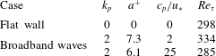
 $c_{p}/u_{\ast }=2$ (slow waves) and 25 (fast waves), and a flat-wall case is also considered for comparison. The flow is driven by a mean pressure gradient to ensure a constant flow rate. The computational parameters are given in table 1.
The free-slip condition is applied at the top boundary, and the bottom boundary condition is provided by the broadband wave motion obtained from the HOS simulation with a  $288\times 288$ grid. The periodic condition is applied in the streamwise and spanwise directions for both the turbulent flow and wave motions. The computational flow domain has a size of
 $(L_{x},L_{y},L_{z})=(2\unicode[STIX]{x03C0}\unicode[STIX]{x1D6FF},\unicode[STIX]{x1D6FF},\unicode[STIX]{x03C0}\unicode[STIX]{x1D6FF})$ with a grid number of
 $(N_{x},N_{y},N_{z})=(192,144,192)$. The grid number is nearly the same as that of the DNS of Yang & Shen (Reference Yang and Shen2017) and higher than that of Yang & Shen (Reference Yang and Shen2010). In particular, uniform grid sizes are used in the streamwise and spanwise directions with
 $\unicode[STIX]{x0394}\unicode[STIX]{x1D709}_{1}^{+}\approx 9.8$ and
 $\unicode[STIX]{x0394}\unicode[STIX]{x1D709}_{3}^{+}\approx 4.9$, respectively, and the vertical grid is stretched from
 $\unicode[STIX]{x0394}\unicode[STIX]{x1D709}_{2,min}^{+}\approx 0.018$ in the vicinity of the wavy boundary to
 $\unicode[STIX]{x0394}\unicode[STIX]{x1D709}_{2,max}^{+}\approx 3.27$ at the top. All simulations are carried out for about 16 000 viscous time units
 $(tu_{\ast }^{2}/\unicode[STIX]{x1D708})$, and the turbulence field has reached a statistically stationary state when the data are collected. Statistics are obtained from 300 instantaneous flow field data with an approximate time interval of 20 viscous time units between each dataset.
In the present study, the turbulence–wave simulation uses a one-way coupling scheme. In other words, the effect of overlying turbulence on surface waves is neglected. The surface wave field evolves in time, and the surface elevation and orbital velocities are provided as the bottom boundary conditions for the simulation of the overlying flow at each computational time step. It should be pointed out that two-way coupling is used when considering the wind-forcing effect on the wave field evolution and wave growth rate (Liu et al. Reference Liu, Yang, Guo and Shen2010; Yang et al. Reference Yang, Meneveau and Shen2014; Hao & Shen Reference Hao and Shen2019). As pointed out by Hao & Shen (Reference Hao and Shen2019), it takes a much longer time of up to  $O(3000)$ peak wave periods for the wave spectrum to show appreciable change, as compared with the turbulent flow scales. For a short duration, the one-way and two-way coupling schemes result in only a slight difference in the wave spectrum for the waves at high wavenumbers (Yang & Shen Reference Yang and Shen2011). Compared with the fast-wave-field case, the influence of the airflow on the slow wave field is greater indeed. But overall, the influence of the airflow on the wave field is still a much longer process compared with the much faster eddy-turnover process in the turbulent airflow above surface waves. The main focus of the present work is the effects of surface waves on the overlying turbulent flow, and consequently the current one-way coupling treatment is adequate for capturing the turbulent flow behaviours under the impact of surface waves (Yang, Meneveau & Shen Reference Yang, Meneveau and Shen2013).
Parameters of the computational set-up, including the dimensionless peak wavenumber  $k_{p}$, the wave amplitude normalized by the wall viscous unit
 $a^{+}$, the wave phase speed normalized by the friction velocity
 $c_{p}/u_{\ast }$ and the Reynolds number
 $Re_{\unicode[STIX]{x1D70F}}$ based on the friction velocity and channel half-width. For broadband waves,
 $a=\sqrt{2}a_{rms}$, where
 $a_{rms}$ denotes the root mean square of wave amplitudes.

2.3 Two-point correlation transport equation in curvilinear coordinates
For inhomogeneous turbulence, the one-point Reynolds stresses transport equation can be employed to describe the turbulent kinetic energy production, dissipation and transport in physical space. However, in order to reveal the scale dependence of the energy transfer process, we resort to the two-point correlation transport equation (Lee & Moser Reference Lee and Moser2015, Reference Lee and Moser2019). In curvilinear coordinates, if we write the equation of velocity fluctuations  $u_{i}^{\prime }$ (including both the turbulent and wave-coherent components) at one point
 $(\unicode[STIX]{x1D709}_{1},\unicode[STIX]{x1D709}_{2},\unicode[STIX]{x1D709}_{3},\unicode[STIX]{x1D70F})$, and multiply it by the velocity fluctuations
 $u_{rj}^{\prime }$ at another point
 $(\unicode[STIX]{x1D709}_{1}+r_{\unicode[STIX]{x1D709}_{1}},\unicode[STIX]{x1D709}_{2},\unicode[STIX]{x1D709}_{3}+r_{\unicode[STIX]{x1D709}_{3}},\unicode[STIX]{x1D70F})$, adding the
 $\unicode[STIX]{x1D709}_{2}$-plane average of this equation to its counterpart with the subscripts exchanged, we can obtain the transport equation of two-point correlation, i.e.
 $$\begin{eqnarray}\frac{\unicode[STIX]{x2202}\overline{u_{i}^{\prime }u_{rj}^{\prime }}}{\unicode[STIX]{x2202}\unicode[STIX]{x1D70F}}(r_{\unicode[STIX]{x1D709}_{1}},\unicode[STIX]{x1D709}_{2},r_{\unicode[STIX]{x1D709}_{3}})=P_{ij}+\unicode[STIX]{x1D6F1}_{s,ij}+T_{t,ij}+T_{p,ij}+T_{v,ij}-\unicode[STIX]{x1D700}_{ij}+A_{ij}.\end{eqnarray}$$
The right-hand side of (2.17) contains the production, pressure-strain, turbulent transport, pressure transport, viscous transport and dissipation terms, which can be expressed, respectively, as follows:
 $$\begin{eqnarray}P_{ij}=-(\overline{u_{rj}^{\prime }v^{\prime }}\unicode[STIX]{x1D6FF}_{i1}+\overline{u_{i}^{\prime }v_{r}^{\prime }}\unicode[STIX]{x1D6FF}_{j1}+\overline{u_{rj}^{\prime }u_{k}^{\prime }\unicode[STIX]{x1D719}_{k}}\unicode[STIX]{x1D6FF}_{i1}+\overline{u_{i}^{\prime }u_{rk}^{\prime }\unicode[STIX]{x1D719}_{rk}}\unicode[STIX]{x1D6FF}_{j1})\frac{\unicode[STIX]{x2202}U}{\unicode[STIX]{x2202}\unicode[STIX]{x1D709}_{2}},\end{eqnarray}$$
 $$\begin{eqnarray}\displaystyle \unicode[STIX]{x1D6F1}_{s,ij} & = & \displaystyle \frac{\unicode[STIX]{x2202}\overline{p^{\prime }u_{rj}^{\prime }}}{\unicode[STIX]{x2202}r_{\unicode[STIX]{x1D709}_{1}}}\unicode[STIX]{x1D6FF}_{i1}-\frac{\unicode[STIX]{x2202}\overline{p_{r}^{\prime }u_{i}^{\prime }}}{\unicode[STIX]{x2202}r_{\unicode[STIX]{x1D709}_{1}}}\unicode[STIX]{x1D6FF}_{j1}+\overline{p^{\prime }\frac{\unicode[STIX]{x2202}u_{rj}^{\prime }}{\unicode[STIX]{x2202}\unicode[STIX]{x1D709}_{2}}}\unicode[STIX]{x1D6FF}_{i2}+\overline{p_{r}^{\prime }\frac{\unicode[STIX]{x2202}u_{i}^{\prime }}{\unicode[STIX]{x2202}\unicode[STIX]{x1D709}_{2}}}\unicode[STIX]{x1D6FF}_{j2}\nonumber\\ \displaystyle & & \displaystyle +\,\frac{\unicode[STIX]{x2202}\overline{p^{\prime }u_{rj}^{\prime }}}{\unicode[STIX]{x2202}r_{\unicode[STIX]{x1D709}_{3}}}\unicode[STIX]{x1D6FF}_{i3}-\overline{\frac{\unicode[STIX]{x2202}p_{r}^{\prime }u_{i}^{\prime }}{\unicode[STIX]{x2202}r_{\unicode[STIX]{x1D709}_{3}}}}\unicode[STIX]{x1D6FF}_{j3}+\overline{p^{\prime }\unicode[STIX]{x1D719}_{i}\frac{\unicode[STIX]{x2202}u_{rj}^{\prime }}{\unicode[STIX]{x2202}\unicode[STIX]{x1D709}_{2}}}+\overline{p_{r}^{\prime }\unicode[STIX]{x1D719}_{rj}\frac{\unicode[STIX]{x2202}u_{i}^{\prime }}{\unicode[STIX]{x2202}\unicode[STIX]{x1D709}_{2}}},\end{eqnarray}$$
 $$\begin{eqnarray}\displaystyle T_{t,ij} & = & \displaystyle \overline{\frac{\unicode[STIX]{x2202}u_{rj}^{\prime }(u_{i}^{\prime }u^{\prime })}{\unicode[STIX]{x2202}r_{\unicode[STIX]{x1D709}_{1}}}}-\overline{\frac{\unicode[STIX]{x2202}u_{i}^{\prime }(u_{rj}^{\prime }u_{r}^{\prime })}{\unicode[STIX]{x2202}r_{\unicode[STIX]{x1D709}_{1}}}}-\overline{u_{rj}^{\prime }\frac{\unicode[STIX]{x2202}u_{i}^{\prime }v^{\prime }}{\unicode[STIX]{x2202}\unicode[STIX]{x1D709}_{2}}}-\overline{u_{i}^{\prime }\frac{\unicode[STIX]{x2202}u_{rj}^{\prime }v_{r}^{\prime }}{\unicode[STIX]{x2202}\unicode[STIX]{x1D709}_{2}}}\nonumber\\ \displaystyle & & \displaystyle +\,\overline{\frac{\unicode[STIX]{x2202}u_{rj}^{\prime }(u_{i}^{\prime }w^{\prime })}{\unicode[STIX]{x2202}r_{\unicode[STIX]{x1D709}_{3}}}}-\overline{\frac{\unicode[STIX]{x2202}u_{i}^{\prime }(u_{rj}^{\prime }w_{r}^{\prime })}{\unicode[STIX]{x2202}r_{\unicode[STIX]{x1D709}_{3}}}}-\overline{u_{rj}^{\prime }\unicode[STIX]{x1D719}_{k}\frac{\unicode[STIX]{x2202}u_{i}^{\prime }u_{k}^{\prime }}{\unicode[STIX]{x2202}\unicode[STIX]{x1D709}_{2}}}-\overline{u_{i}^{\prime }\unicode[STIX]{x1D719}_{rk}\frac{\unicode[STIX]{x2202}u_{rj}^{\prime }u_{rk}^{\prime }}{\unicode[STIX]{x2202}\unicode[STIX]{x1D709}_{2}}},\end{eqnarray}$$
 $$\begin{eqnarray}\displaystyle & \displaystyle T_{p,ij}=-\overline{\frac{\unicode[STIX]{x2202}p^{\prime }u_{rj}^{\prime }}{\unicode[STIX]{x2202}\unicode[STIX]{x1D709}_{2}}}\unicode[STIX]{x1D6FF}_{i2}-\overline{\frac{\unicode[STIX]{x2202}p_{r}^{\prime }u_{i}^{\prime }}{\unicode[STIX]{x2202}\unicode[STIX]{x1D709}_{2}}}\unicode[STIX]{x1D6FF}_{j2}-\overline{\unicode[STIX]{x1D719}_{i}\frac{\unicode[STIX]{x2202}p^{\prime }u_{rj}^{\prime }}{\unicode[STIX]{x2202}\unicode[STIX]{x1D709}_{2}}}-\overline{\unicode[STIX]{x1D719}_{rj}\frac{\unicode[STIX]{x2202}p_{r}^{\prime }u_{i}^{\prime }}{\unicode[STIX]{x2202}\unicode[STIX]{x1D709}_{2}}}, & \displaystyle\end{eqnarray}$$
 $$\begin{eqnarray}\displaystyle & \displaystyle T_{\unicode[STIX]{x1D708},ij}=\unicode[STIX]{x1D708}\overline{\frac{\unicode[STIX]{x2202}^{2}u_{i}^{\prime }u_{rj}^{\prime }}{\unicode[STIX]{x2202}\unicode[STIX]{x1D709}_{2}\unicode[STIX]{x2202}\unicode[STIX]{x1D709}_{2}}}+2\unicode[STIX]{x1D708}\overline{\unicode[STIX]{x1D719}_{2}\frac{\unicode[STIX]{x2202}}{\unicode[STIX]{x2202}\unicode[STIX]{x1D709}_{2}}\left(u_{rj}^{\prime }\frac{\unicode[STIX]{x2202}u_{i}^{\prime }}{\unicode[STIX]{x2202}\unicode[STIX]{x1D709}_{2}}\right)}+2\unicode[STIX]{x1D708}\overline{\unicode[STIX]{x1D719}_{r2}\frac{\unicode[STIX]{x2202}}{\unicode[STIX]{x2202}\unicode[STIX]{x1D709}_{2}}\left(u_{i}^{\prime }\frac{\unicode[STIX]{x2202}u_{rj}^{\prime }}{\unicode[STIX]{x2202}\unicode[STIX]{x1D709}_{2}}\right)}+\unicode[STIX]{x1D713}_{T_{\unicode[STIX]{x1D708},ij}}, & \displaystyle\end{eqnarray}$$
 $$\begin{eqnarray}\displaystyle & \displaystyle \unicode[STIX]{x1D700}_{ij}=2\unicode[STIX]{x1D708}\overline{\frac{\unicode[STIX]{x2202}^{2}u_{i}^{\prime }u_{rj}^{\prime }}{\unicode[STIX]{x2202}r_{\unicode[STIX]{x1D709}_{1}}\unicode[STIX]{x2202}r_{\unicode[STIX]{x1D709}_{1}}}}-2\unicode[STIX]{x1D708}\overline{\frac{\unicode[STIX]{x2202}u_{i}^{\prime }}{\unicode[STIX]{x2202}\unicode[STIX]{x1D709}_{2}}\frac{\unicode[STIX]{x2202}u_{rj}^{\prime }}{\unicode[STIX]{x2202}\unicode[STIX]{x1D709}_{2}}}+2\unicode[STIX]{x1D708}\overline{\frac{\unicode[STIX]{x2202}^{2}u_{i}^{\prime }u_{rj}^{\prime }}{\unicode[STIX]{x2202}r_{\unicode[STIX]{x1D709}_{3}}\unicode[STIX]{x2202}r_{\unicode[STIX]{x1D709}_{3}}}}-2\unicode[STIX]{x1D708}\overline{(\unicode[STIX]{x1D719}_{2}+\unicode[STIX]{x1D719}_{r2})\frac{\unicode[STIX]{x2202}u_{i}^{\prime }}{\unicode[STIX]{x2202}\unicode[STIX]{x1D709}_{2}}\frac{\unicode[STIX]{x2202}u_{rj}^{\prime }}{\unicode[STIX]{x2202}\unicode[STIX]{x1D709}_{2}}}+\unicode[STIX]{x1D713}_{\unicode[STIX]{x1D700}_{ij}}, & \displaystyle\end{eqnarray}$$
 $$\begin{eqnarray}\displaystyle A_{ij} & = & \displaystyle -(\overline{u_{rj}^{\prime }\unicode[STIX]{x1D719}_{1}}\unicode[STIX]{x1D6FF}_{i1}+\overline{u_{i}^{\prime }\unicode[STIX]{x1D719}_{r1}}\unicode[STIX]{x1D6FF}_{j1})\frac{\unicode[STIX]{x2202}\bar{u}\bar{u}}{\unicode[STIX]{x2202}\unicode[STIX]{x1D709}_{2}}-(\overline{u_{rj}^{\prime }\unicode[STIX]{x1D719}_{i}}+\overline{u_{i}^{\prime }\unicode[STIX]{x1D719}_{rj}})\frac{\unicode[STIX]{x2202}\bar{p}}{\unicode[STIX]{x2202}\unicode[STIX]{x1D709}_{2}}\nonumber\\ \displaystyle & & \displaystyle +\,2\unicode[STIX]{x1D708}(\overline{\unicode[STIX]{x1D719}_{2}u_{rj}^{\prime }\unicode[STIX]{x1D6FF}_{i1}}+\overline{\unicode[STIX]{x1D719}_{r2}u_{i}^{\prime }\unicode[STIX]{x1D6FF}_{j1}})\frac{\unicode[STIX]{x2202}^{2}\bar{u}}{\unicode[STIX]{x2202}\unicode[STIX]{x1D709}_{2}\unicode[STIX]{x2202}\unicode[STIX]{x1D709}_{2}},\end{eqnarray}$$
where the overbar denotes the ensemble average on a curved plane of the wave-boundary-fitted grid and over time. In addition, it should be noted that the viscous transport and dissipation terms only consider the principal parts here, where  $\unicode[STIX]{x1D713}_{ij}$ denotes the viscous cross terms as a result of coordinate transformation and
 $A_{ij}$ denotes the additional terms due to the effects of boundary deformation on the mean flow. Note that this ensemble average allows us to quantify the statistical properties of the flow in the thin viscous sublayer very close to the wavy surface as has been used in previous studies of turbulent flows over waves (Sullivan et al. Reference Sullivan, McWilliams and Moeng2000; Kihara et al. Reference Kihara, Hanazaki, Mizuya and Ueda2007; Yang & Shen Reference Yang and Shen2017). If averaging on the Cartesian grid on a horizontal plane is applied, regions below the wave crest cannot be accounted for (see e.g. the discussion in Rutgersson & Sullivan (Reference Rutgersson and Sullivan2005)). We find the difference between the results calculated from these two averaging methods to be small at a short distance above the wave crest and it becomes negligible as the surface-fitted grid becomes flatter at higher elevations.
Furthermore, the turbulent transport term  $T_{t,ij}$ can be decomposed into two parts as follows:
 $$\begin{eqnarray}\displaystyle & \displaystyle T_{t,ij}=T_{t,ij}^{\unicode[STIX]{x1D6FC}}+T_{t,ij}^{\unicode[STIX]{x1D6FD}}, & \displaystyle\end{eqnarray}$$
 $$\begin{eqnarray}\displaystyle & \displaystyle T_{t,ij}^{\unicode[STIX]{x1D6FC}}=-\frac{1}{2}\frac{\unicode[STIX]{x2202}\overline{u_{rj}^{\prime }(u_{i}^{\prime }v^{\prime })}}{\unicode[STIX]{x2202}\unicode[STIX]{x1D709}_{2}}-\frac{1}{2}\frac{\unicode[STIX]{x2202}\overline{u_{i}^{\prime }(u_{rj}^{\prime }v_{r}^{\prime })}}{\unicode[STIX]{x2202}\unicode[STIX]{x1D709}_{2}}-\frac{1}{2}\overline{\unicode[STIX]{x1D719}_{k}\frac{\unicode[STIX]{x2202}u_{rj}^{\prime }(u_{i}^{\prime }u_{k}^{\prime })}{\unicode[STIX]{x2202}\unicode[STIX]{x1D709}_{2}}}-\frac{1}{2}\overline{\unicode[STIX]{x1D719}_{rk}\frac{\unicode[STIX]{x2202}u_{i}^{\prime }(u_{rj}^{\prime }u_{rk}^{\prime })}{\unicode[STIX]{x2202}\unicode[STIX]{x1D709}_{2}}}, & \displaystyle\end{eqnarray}$$
 $$\begin{eqnarray}\displaystyle T_{t,ij}^{\unicode[STIX]{x1D6FD}} & = & \displaystyle \overline{\frac{\unicode[STIX]{x2202}u_{rj}^{\prime }(u_{i}^{\prime }u^{\prime })}{\unicode[STIX]{x2202}r_{\unicode[STIX]{x1D709}_{1}}}}-\overline{\frac{\unicode[STIX]{x2202}u_{i}^{\prime }(u_{rj}^{\prime }u_{r}^{\prime })}{\unicode[STIX]{x2202}r_{\unicode[STIX]{x1D709}_{1}}}}+\overline{\frac{\unicode[STIX]{x2202}u_{rj}^{\prime }(u_{i}^{\prime }w^{\prime })}{\unicode[STIX]{x2202}r_{\unicode[STIX]{x1D709}_{3}}}}-\overline{\frac{\unicode[STIX]{x2202}u_{i}^{\prime }(u_{rj}^{\prime }w_{r}^{\prime })}{\unicode[STIX]{x2202}r_{\unicode[STIX]{x1D709}_{3}}}}\nonumber\\ \displaystyle & & \displaystyle -\,\frac{1}{2}\frac{\unicode[STIX]{x2202}\overline{u_{rj}^{\prime }(u_{i}^{\prime }v^{\prime })}}{\unicode[STIX]{x2202}\unicode[STIX]{x1D709}_{2}}-\frac{1}{2}\frac{\unicode[STIX]{x2202}\overline{u_{i}^{\prime }(u_{rj}^{\prime }v_{r}^{\prime })}}{\unicode[STIX]{x2202}\unicode[STIX]{x1D709}_{2}}+\overline{(u_{i}^{\prime }v^{\prime })\frac{\unicode[STIX]{x2202}u_{rj}^{\prime }}{\unicode[STIX]{x2202}\unicode[STIX]{x1D709}_{2}}}+\overline{(u_{rj}^{\prime }v_{r}^{\prime })\frac{\unicode[STIX]{x2202}u_{i}^{\prime }}{\unicode[STIX]{x2202}\unicode[STIX]{x1D709}_{2}}}\nonumber\\ \displaystyle & & \displaystyle -\,\frac{1}{2}\overline{\unicode[STIX]{x1D719}_{k}\frac{\unicode[STIX]{x2202}u_{rj}^{\prime }(u_{i}^{\prime }u_{k}^{\prime })}{\unicode[STIX]{x2202}\unicode[STIX]{x1D709}_{2}}}-\frac{1}{2}\overline{\unicode[STIX]{x1D719}_{rk}\frac{\unicode[STIX]{x2202}u_{i}^{\prime }(u_{rj}^{\prime }u_{rk}^{\prime })}{\unicode[STIX]{x2202}\unicode[STIX]{x1D709}_{2}}}+\overline{u_{i}^{\prime }u_{k}^{\prime }\unicode[STIX]{x1D719}_{k}\frac{\unicode[STIX]{x2202}u_{rj}^{\prime }}{\unicode[STIX]{x2202}\unicode[STIX]{x1D709}_{2}}}+\overline{u_{rj}^{\prime }u_{rk}^{\prime }\unicode[STIX]{x1D719}_{rk}\frac{\unicode[STIX]{x2202}u_{i}^{\prime }}{\unicode[STIX]{x2202}\unicode[STIX]{x1D709}_{2}}},\end{eqnarray}$$
where  $T_{t,ij}^{\unicode[STIX]{x1D6FD}}$ satisfies
 $$\begin{eqnarray}\lim _{\substack{ r_{\unicode[STIX]{x1D709}_{1}}\rightarrow 0 \\ r_{\unicode[STIX]{x1D709}_{3}}\rightarrow 0}}T_{t,ij}^{\unicode[STIX]{x1D6FD}}=0,\quad \forall \unicode[STIX]{x1D709}_{2}.\end{eqnarray}$$
Therefore,  $T_{t,ij}^{\unicode[STIX]{x1D6FD}}$ can be interpreted as the inter-scale energy transfer and does not contribute to the net spatial energy flux (see appendix A). Hereafter,
 $T_{t,ij}^{\unicode[STIX]{x1D6FD}}$ is referred to as the inter-scale turbulent transport and
 $T_{t,ij}^{\unicode[STIX]{x1D6FC}}$ is called the spatial turbulent transport. Note that the nonlinear term decomposition is not unique. The present spatial and inter-scale parts depicted in (2.26) and (2.27) are consistent with the decomposition adopted by Mizuno (Reference Mizuno2016) and Lee & Moser (Reference Lee and Moser2019) for flat-wall turbulence. It should be noted that although the energy transfer between vertical scales is also important for understanding wall-bounded turbulence, it is beyond the scope of the present work. It may be better to investigate the energy distribution on vertical scales based on the generalized Kolmogorov equation, as recently studied by Cimarelli et al. (Reference Cimarelli, De Angelis, Jiménez and Casciola2016).
By performing a Fourier transform in the  $\unicode[STIX]{x1D709}_{1}$ and
 $\unicode[STIX]{x1D709}_{3}$ directions, equation (2.17) becomes
 $$\begin{eqnarray}\frac{\unicode[STIX]{x2202}\hat{E}_{ij}}{\unicode[STIX]{x2202}\unicode[STIX]{x1D70F}}(k_{\unicode[STIX]{x1D709}_{1}},\unicode[STIX]{x1D709}_{2},k_{\unicode[STIX]{x1D709}_{3}})=\hat{E}_{ij}^{P}+\hat{E}_{ij}^{\unicode[STIX]{x1D6F1}_{s}}+\hat{E}_{ij}^{T_{t}^{\unicode[STIX]{x1D6FC}}}+\hat{E}_{ij}^{T_{t}^{\unicode[STIX]{x1D6FD}}}+\hat{E}_{ij}^{T_{p}}+\hat{E}_{ij}^{T_{\unicode[STIX]{x1D708}}}-\hat{E}_{ij}^{\unicode[STIX]{x1D700}}+\hat{E}_{ij}^{A},\end{eqnarray}$$
where each term is the Fourier transform of its counterpart in (2.17). The one-dimensional energy spectrum is defined as
 $$\begin{eqnarray}E_{ij}(k_{\unicode[STIX]{x1D709}_{1}},\unicode[STIX]{x1D709}_{2})=\mathop{\sum }_{k_{\unicode[STIX]{x1D709}_{3}}}[\hat{E}_{ij}(k_{\unicode[STIX]{x1D709}_{1}},\unicode[STIX]{x1D709}_{2},k_{\unicode[STIX]{x1D709}_{3}})+\hat{E}_{ij}(-k_{\unicode[STIX]{x1D709}_{1}},\unicode[STIX]{x1D709}_{2},k_{\unicode[STIX]{x1D709}_{3}})]\end{eqnarray}$$
or
 $$\begin{eqnarray}E_{ij}(k_{\unicode[STIX]{x1D709}_{3}},\unicode[STIX]{x1D709}_{2})=\mathop{\sum }_{k_{\unicode[STIX]{x1D709}_{1}}}[\hat{E}_{ij}(k_{\unicode[STIX]{x1D709}_{1}},\unicode[STIX]{x1D709}_{2},k_{\unicode[STIX]{x1D709}_{3}})+\hat{E}_{ij}(k_{\unicode[STIX]{x1D709}_{1}},\unicode[STIX]{x1D709}_{2},-k_{\unicode[STIX]{x1D709}_{3}})],\end{eqnarray}$$
and similarly for the other terms. Then, the transport equation of the one-dimensional energy spectrum  $E_{ij}$ is obtained as
 $$\begin{eqnarray}\frac{\unicode[STIX]{x2202}E_{ij}}{\unicode[STIX]{x2202}\unicode[STIX]{x1D70F}}=E_{p,ij}+E_{\unicode[STIX]{x1D6F1}_{s},ij}+E_{T_{t}^{\unicode[STIX]{x1D6FC}},ij}+E_{T_{t}^{\unicode[STIX]{x1D6FD}},ij}+E_{T_{p},ij}+E_{T_{\unicode[STIX]{x1D708}},ij}-E_{\unicode[STIX]{x1D700},ij}+E_{A,ij}.\end{eqnarray}$$
Further analysis of the terms in (2.32) is presented in § 3, which describes the processes of how energy is produced, dissipated and transported among different scales and locations, and provides a general turbulent energy transfer framework in the presence of surface waves. Note that  $E_{ij}$ is a function of
 $\unicode[STIX]{x1D709}_{2}$, which represents the mean vertical distance away from the wave surface, i.e.
 $\overline{y}=\unicode[STIX]{x1D709}_{2}$. In the following, we omit the overbar and use
 $y$ to indicate the vertical distance without special note for brevity. The streamwise and spanwise wavenumbers are denoted by
 $k_{1}$ and
 $k_{3}$, respectively, in the computational domain, and
 $\unicode[STIX]{x1D706}_{1}$ and
 $\unicode[STIX]{x1D706}_{3}$ are the corresponding streamwise and spanwise wavelengths.
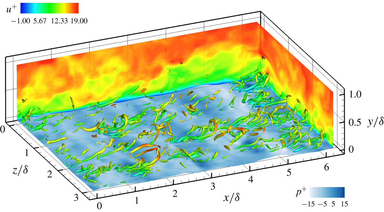
Illustration of the three-dimensional flow field over surface waves for the case of  $c_{p}/u_{\ast }=2$. Contours of the instantaneous streamwise velocity are plotted in the
 $x$–
 $y$ plane and the
 $y$–
 $z$ plane. The distribution of the turbulent flow pressure on the wave surface is also shown. The vortical structures are identified by the isosurface of 10 % of the maximum
 $\unicode[STIX]{x1D706}_{ci}$ and coloured by the instantaneous streamwise velocity.

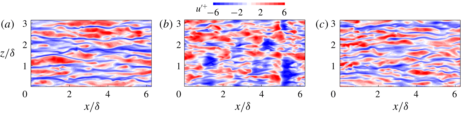
Instantaneous streamwise velocity fluctuation in the  $x$–
 $z$ plane located at
 $y^{+}=12$: (a) the flat-wall case; (b)
 $c_{p}/u_{\ast }=2$; (c)
 $c_{p}/u_{\ast }=25$.

3 Results and discussion
3.1 Flow visualization
Before discussing the turbulence statistics, it is instructive to examine the instantaneous turbulence field over water waves from visualization of the data generated by the DNS–HOS simulation. Taking the slow-wave case of  $c_{p}/u_{\ast }=2$ as an example, figure 2 shows the three-dimensional instantaneous flow field. The distribution of the turbulent flow pressure on the wave surface is closely related to the surface slope with generally positive (negative) values on the windward (leeward) side. The overlying vortical structures are visualized via the isosurface of the local swirling strength
 $\unicode[STIX]{x1D706}_{ci}$ (Zhou et al. Reference Zhou, Adrian, Balachandar and Kendall1999). As shown in the figure, they are dominated by the quasi-streamwise vortices and affected by the surface waves. The streamwise size of these vortices is constrained by the dominant wavelength and the inclination angle is modulated by the waveform, as suggested by Yang & Shen (Reference Yang and Shen2009). The contours of the streamwise velocity in the
 $x$–
 $y$ plane are tilted downstream in the near-surface region, consistent with the posture of the streamwise vortices. Note that the low-speed zones are lifted up in the
 $y$–
 $z$ plane, corresponding to the formation of streaky structures.
Figure 3 shows the instantaneous contours of the streamwise velocity fluctuations in the  $x$–
 $z$ plane located at
 $y^{+}=12$. For the flat-wall case, the flow pattern in figure 3(a) is dominated by the streamwise elongated low-speed streaks. In the presence of the surface waves, the typical flat-wall streaky structures are disrupted by the periodic wave motions. As shown in figure 3(b), the velocity fluctuation alternates in sign in the streamwise direction with the spatial periodicity corresponding to the dominant wavelength
 $\unicode[STIX]{x1D706}_{p}$. As the wave age increases to
 $c_{p}/u_{\ast }=25$, the effect of the surface waves on the flow structure is greatly attenuated, and the streaky structures similar to the flat-wall turbulence case (figure 3a) are recovered in figure 3(c). These results show clearly the impact of surface waves on the turbulent flow field above. The effects on turbulent energy are analysed in detail in the following subsections.
3.2 Energy spectra
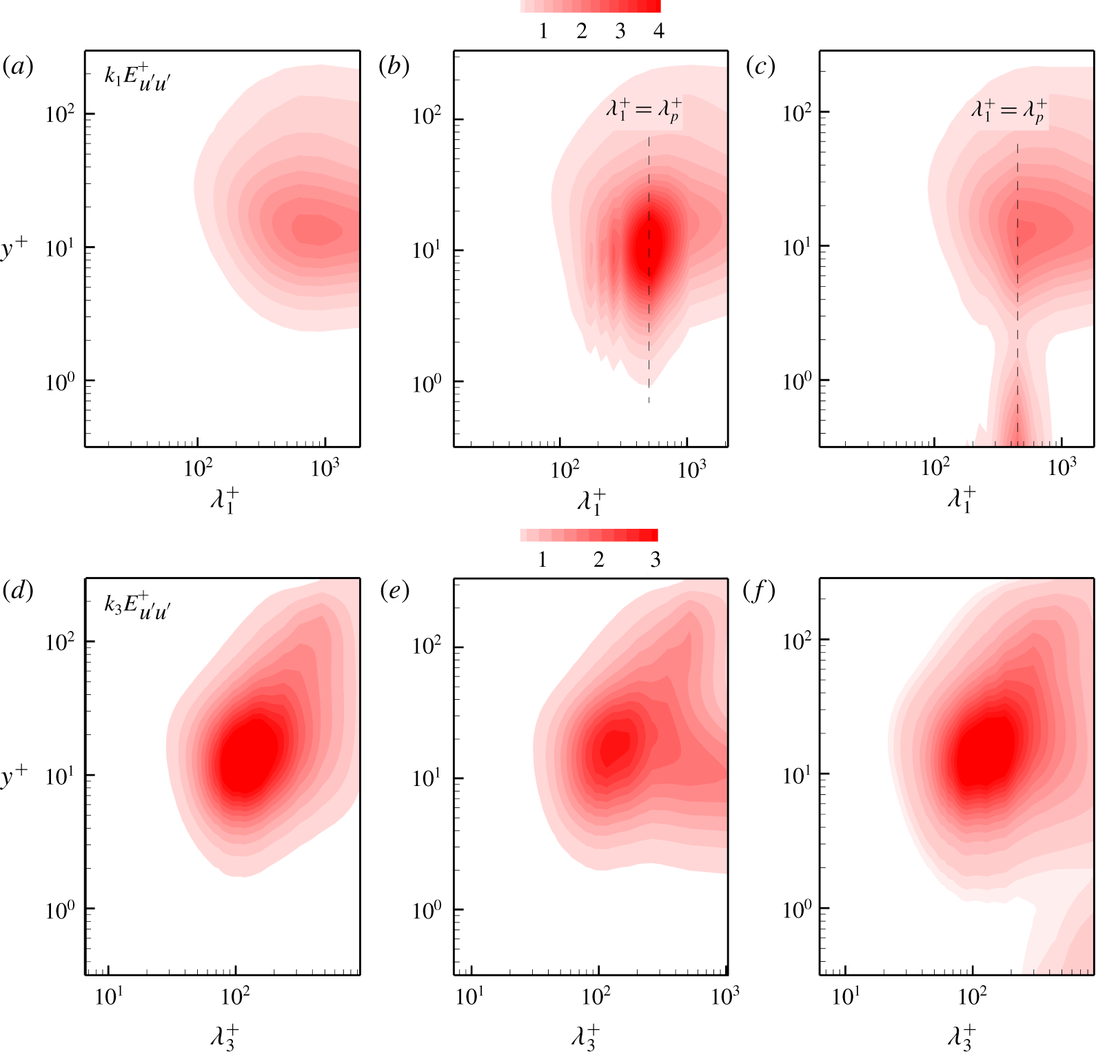
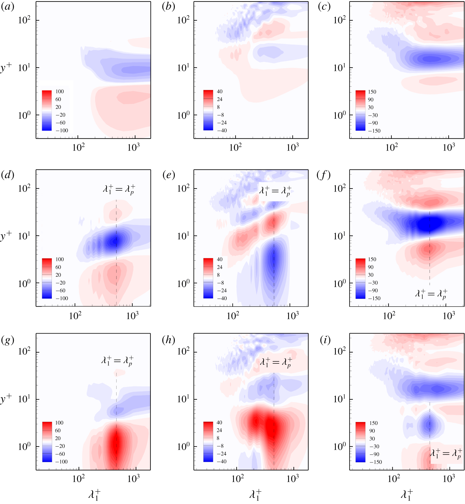
The main objective of the present study is to explore the turbulent energy transfer process under the impact of surface waves. We begin by examining the energy distribution at different length scales and vertical locations. The one-dimensional premultiplied energy spectra of the streamwise velocity fluctuations on the plane of the streamwise wavelength  $\unicode[STIX]{x1D706}_{1}$ (or the spanwise wavelength
 $\unicode[STIX]{x1D706}_{3}$) and
 $y$ are plotted in figure 4. For the flat-wall case, the spectral peaks in figures 4(a) and 4(d) are consistent with the results of Marusic, Mathis & Hutchins (Reference Marusic, Mathis and Hutchins2010) and Smits, McKeon & Marusic (Reference Smits, McKeon and Marusic2011). The peaks denote the streamwise length (
 $\unicode[STIX]{x1D706}_{1}^{+}\approx 1000$) and the spanwise spacing (
 $\unicode[STIX]{x1D706}_{3}^{+}\approx 100$) of the low-speed streaky structures in the buffer region (see figure 3a), which are important elements of the near-wall self-sustaining process as described by Hamilton, Kim & Waleffe (Reference Hamilton, Kim and Waleffe1995) and Jiménez & Pinelli (Reference Jiménez and Pinelli1999). For the slow-wave-field case of
 $c_{p}/u_{\ast }=2$, as seen in figure 4(b), the streamwise length scale of the peak in the buffer region becomes the wavelength of dominant surface wave,
 $\unicode[STIX]{x1D706}_{p}^{+}\approx 524.8$. In addition, energy is also concentrated at the harmonic wavelengths (figure 4b), significantly different from the flat-wall case. In other words, the original low-speed streaky structures are disrupted by the surface waves, as seen in figure 3(b) and previously observed by Sullivan et al. (Reference Sullivan, McWilliams and Moeng2000). As the wave age increases to
 $c_{p}/u_{\ast }=25$ (figure 4c), in the fast-wave-field case, the streamwise energy spectrum protrudes from the wavy boundary over a range of scales, centring around the dominant wavelength, which can be attributed to the direct contribution of the surface waves to the streamwise Reynolds stress. In the buffer region, the peak position still occurs at the dominant wavelength scale, but its energy amplitude is much smaller than that in the slow-wave case shown in figure 4(b). This result indicates that the streaky structures are not obviously altered by the surface waves when the wave age is large, consistent with figure 3(c). Furthermore, the one-dimensional spanwise premultiplied energy spectra of the streamwise velocity fluctuations are compared in figure 4(d–f). For the case of
 $c_{p}/u_{\ast }=2$, a tip of the spanwise energy spectrum occurs at
 $\unicode[STIX]{x1D706}_{3}^{+}\approx 500$ in the region of
 $y^{+}\approx 100$ as seen in figure 4(e), indicating that the large-scale motion is enhanced by the slow wave. Similar effects of a stationary wavy boundary on the large-scale structures in a turbulent flow were observed in the experimental study by Kuhn, Wagner & von Rohr (Reference Kuhn, Wagner and von Rohr2007). As the wave age increases to
 $c_{p}/u_{\ast }=25$ (figure 4f), the large-scale outer peak is weakened, while an additional local peak region at the surface is observed. The large-scale motions in the very-near-surface region as seen in figure 4(f) correspond to the dynamically evolving surface waves, whose dominant component extends to the whole domain in the spanwise direction. After multiplying the spanwise energy spectra by the spanwise wavenumber
 $k_{3}$, a large-scale spectral peak occurs near the surface.
One-dimensional streamwise (a–c) and spanwise (d–f) premultiplied energy spectra of the streamwise velocity fluctuations: (a,d) the flat-wall case; (b,e)  $c_{p}/u_{\ast }=2$; (c,f)
 $c_{p}/u_{\ast }=25$.

As discussed above, the surface waves have significant influence on the distribution of the turbulent kinetic energy in both physical and spectral spaces. In the following subsections, the premultiplied one-dimensional spectra of the different terms in (2.32) are examined to further explore the underlying mechanism of how surface waves affect the overlying turbulent flow at different length scales and vertical positions.
3.3 Energy production
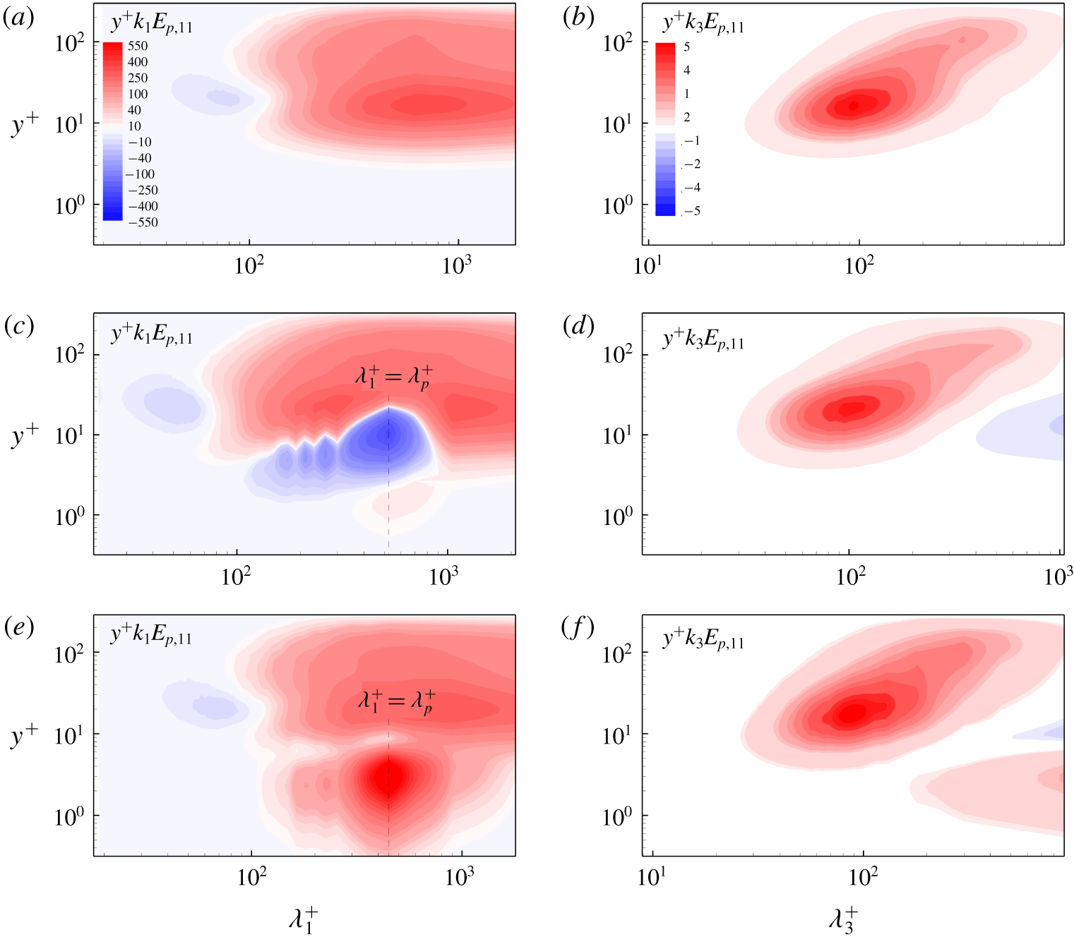
Figure 5 shows the premultiplied one-dimensional streamwise and spanwise spectra of the production term  $E_{p,11}$ of the two-point correlation
 $\overline{u^{\prime }u_{r}^{\prime }}$ in (2.32). For the flat-wall case, as seen in figures 5(a) and 5(b), there is a peak in the buffer region with the streamwise and spanwise length scales corresponding to the typical near-wall streaks. Turbulence is most active in the peak region and the turbulent fluctuations gain energy from the mean shear flow. In addition to the positive production at most length scales and vertical locations, it should be noted that there is a small region where the streamwise spectrum of the production term is negative near
 $y^{+}\approx 20$ and
 $\unicode[STIX]{x1D706}_{1}^{+}\approx 73.6$ in figure 5(a), while no negative region appears in the spanwise spectrum as shown in figure 5(b). This weak negative region is related to the positive co-spectrum of
 $\overline{u^{\prime }v^{\prime }}$, as observed in Lee & Moser (Reference Lee and Moser2015, Reference Lee and Moser2019) at a higher Reynolds number
 $Re_{\unicode[STIX]{x1D70F}}=5200$.
The  $y$- and
 $k$-premultiplied one-dimensional streamwise (a,c,e) and spanwise (b,d,f) spectra of
 $E_{p,11}$: (a,b) the flat-wall case; (c,d)
 $c_{p}/u_{\ast }=2$; (e,f)
 $c_{p}/u_{\ast }=25$.

In the presence of the progressive surface waves, the production term  $E_{p,11}$ retains the main characteristics of the flat-wall case above the buffer region. However, there are significant differences in the region of
 $y^{+}<20$. For the case of
 $c_{p}/u_{\ast }=2$, as seen in figure 5(c), a series of negative spectral peaks appear in the buffer region, corresponding to the length scales of the dominant wave and its harmonic waves. In this case, the motions associated with the surface waves act as energy sinks, extracting energy from the fluctuating field to the mean flow. A quadrant analysis indicates that in the presence of surface waves (results not shown here), the contribution from the Q1 and Q3 events is increased significantly in the near-surface region of
 $y^{+}<10$ due to the wave-induced motions, as compared with the flat-wall case, corresponding to the negative region near the dominant wavelength in figure 5(c). Similarly, the spanwise spectrum shown in figure 5(d) has a large-scale negative region in the region of
 $y^{+}\approx 10$, with the large spanwise length scale reflecting the quasi-two-dimensional characteristics of the broadband wave field. When the wave age increases to
 $c_{p}/u_{\ast }=25$, the streamwise spectrum of the production term plotted in figure 5(e) shows a positive region at the dominant wavelength scale in the region of
 $y^{+}<10$, and contributions of its harmonics to the energy production also emerge. In addition, a positive region near the surface is also observed in figure 5(f), indicating the effect of the wave-induced vertical momentum flux, based on the definition of the production term (2.18) and as further analysed below. It becomes negative at large spanwise length scale similar to the slow-wave case (figure 5d) with an increase of height.
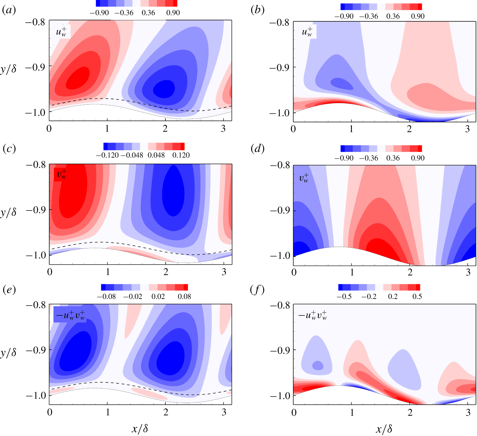
Dominant wave-induced streamwise (a,b) and vertical (c,d) velocity fluctuations, and vertical momentum flux (e,f): (a,c,e)  $c_{p}/u_{\ast }=2$; (b,d,f)
 $c_{p}/u_{\ast }=25$. The dashed line in (a,c,e) denotes the critical layer.

To explain the change of the streamwise spectrum of the production term at the dominant wavelength scale for the different wave age cases shown above, the wave-coherent and turbulent velocities are decomposed to investigate the wave–turbulence interactions (Thais & Magnaudet Reference Thais and Magnaudet1996; Siddiqui & Loewen Reference Siddiqui and Loewen2007). Here, the phase-average approach (Hussain & Reynolds Reference Hussain and Reynolds1970) based on the dominant wavelength is used to perform further analysis. For this purpose, the dominant wave mode is extracted from the instantaneous wave field, and then the corresponding surface deformation and phase information of the dominant wave are obtained. The phase-averaged velocity  $\langle \boldsymbol{u}\rangle$ is obtained based on three steps of averaging. First, the velocity is averaged over time in the frame moving with the dominant wave such that its wave phase is fixed. Then the velocity is averaged in the spanwise direction. Finally, the velocity is averaged over all of the dominant waves in the streamwise direction. Based on the phase-averaged velocity
 $\langle \boldsymbol{u}\rangle$, we define the dominant wave-induced velocity fluctuation
 $\boldsymbol{u}_{w}$ as the fluctuation of
 $\langle \boldsymbol{u}\rangle$ relative to the ensemble average
 $\bar{\boldsymbol{u}}$, i.e.
 $\boldsymbol{u}_{w}=\langle \boldsymbol{u}\rangle -\bar{\boldsymbol{u}}$. The dominant wave-induced velocity fluctuation
 $(u_{w},v_{w})$ and the dominant wave-induced vertical momentum flux,
 $-u_{w}v_{w}$, are plotted in figure 6. The critical layer, where
 $\langle u\rangle =c_{p}$, has been found to be important to the wave-induced motions in field observations (Hristov et al. Reference Hristov, Miller and Friehe2003; Grare et al. Reference Grare, Lenain and Melville2013) and is marked in figure 6(a,c,e). For the case of
 $c_{p}/u_{\ast }=2$, the dominant wave-induced streamwise velocity fluctuation
 $u_{w}$ (figure 6a) is positive on the windward side and negative on the leeward side, while the vertical velocity fluctuation
 $v_{w}$ (figure 6c) on the surface has the opposite distribution, in accordance with the airflow measurements in the laboratory (Buckley & Veron Reference Buckley and Veron2016, Reference Buckley and Veron2019). Consequently, the dominant wave-induced vertical momentum flux is positive below the critical layer height
 $y^{+}\approx 2.5$ (figure 6e), which agrees with the result of Sullivan et al. (Reference Sullivan, McWilliams and Moeng2000) in their study of monochromatic waves, and has a positive contribution to the production term (2.18). Although the result in figure 18 of Sullivan et al. (Reference Sullivan, McWilliams and Moeng2000) corresponds to a wave age of
 $c_{p}/u_{\ast }=3.9$, slightly larger than the present slow-wave age
 $c_{p}/u_{\ast }=2$, the wave-correlated momentum flux across the critical layer is quite similar to that observed in the present study. As the vertical distance from the surface increases,
 $v_{w}$ has an abrupt phase shift across the critical layer, with a positive peak above the crest and a negative peak above the trough. As a result of this phase change, the momentum flux changes its sign in the vertical direction and has a large negative value at the dominant wavelength scale (figure 6e). As the wave age increases to
 $c_{p}/u_{\ast }=25$, the critical layer moves far away from the surface (beyond the vertical extent of the computational domain) and has negligible influence on the wave-induced velocity fluctuations near the surface. As shown in figure 6(b), the distribution of
 $u_{w}$ is tilted with its negative peak moving from the trough region to the crest due to the rapid propagation of surface waves, while the distribution of
 $v_{w}$ remains largely unchanged as the vertical height increases (figure 6d). As a result, positive vertical momentum flux exists in most of the near-surface region and it changes its sign as
 $y$ increases (figure 6f). Therefore, the contribution of the surface waves to energy production varies with the distance away from the surface for different wave ages through the wave-induced vertical momentum flux, according to the definition of the production term (2.18).
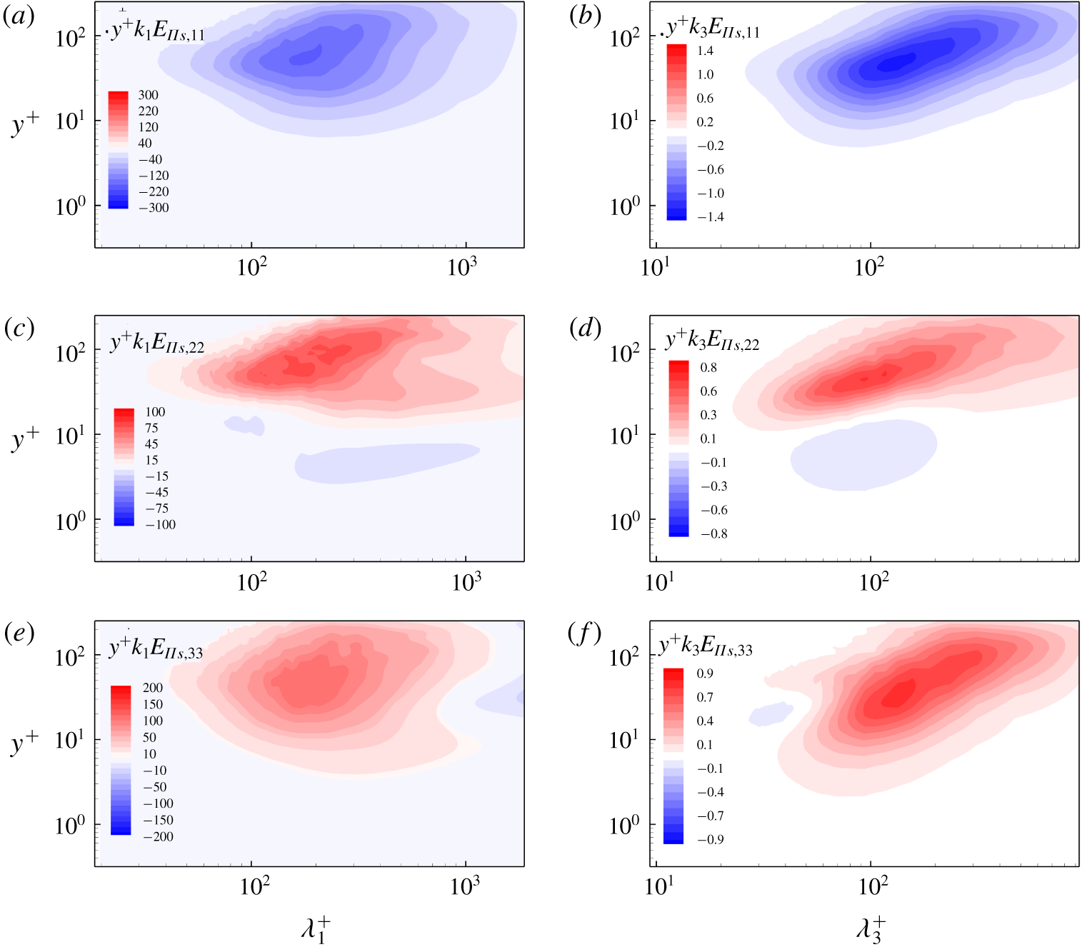
The  $y$- and
 $k$-premultiplied one-dimensional streamwise (a,c,e) and spanwise (b,d,f) spectra of the pressure-strain terms of different velocity components for the flat-wall case: (a,b)
 $E_{\unicode[STIX]{x1D6F1}_{s},11}$; (c,d)
 $E_{\unicode[STIX]{x1D6F1}_{s},22}$; (e,f)
 $E_{\unicode[STIX]{x1D6F1}_{s},33}$.

3.4 Inter-component energy transfer
Due to the incompressibility of the flow field, the spectra of the pressure-strain terms of the different velocity components satisfy
 $$\begin{eqnarray}\hat{E}_{\unicode[STIX]{x1D6F1}_{s},11}+\hat{E}_{\unicode[STIX]{x1D6F1}_{s},22}+\hat{E}_{\unicode[STIX]{x1D6F1}_{s},33}=0\quad \forall (k_{1},\unicode[STIX]{x1D709}_{2},k_{3}),\end{eqnarray}$$
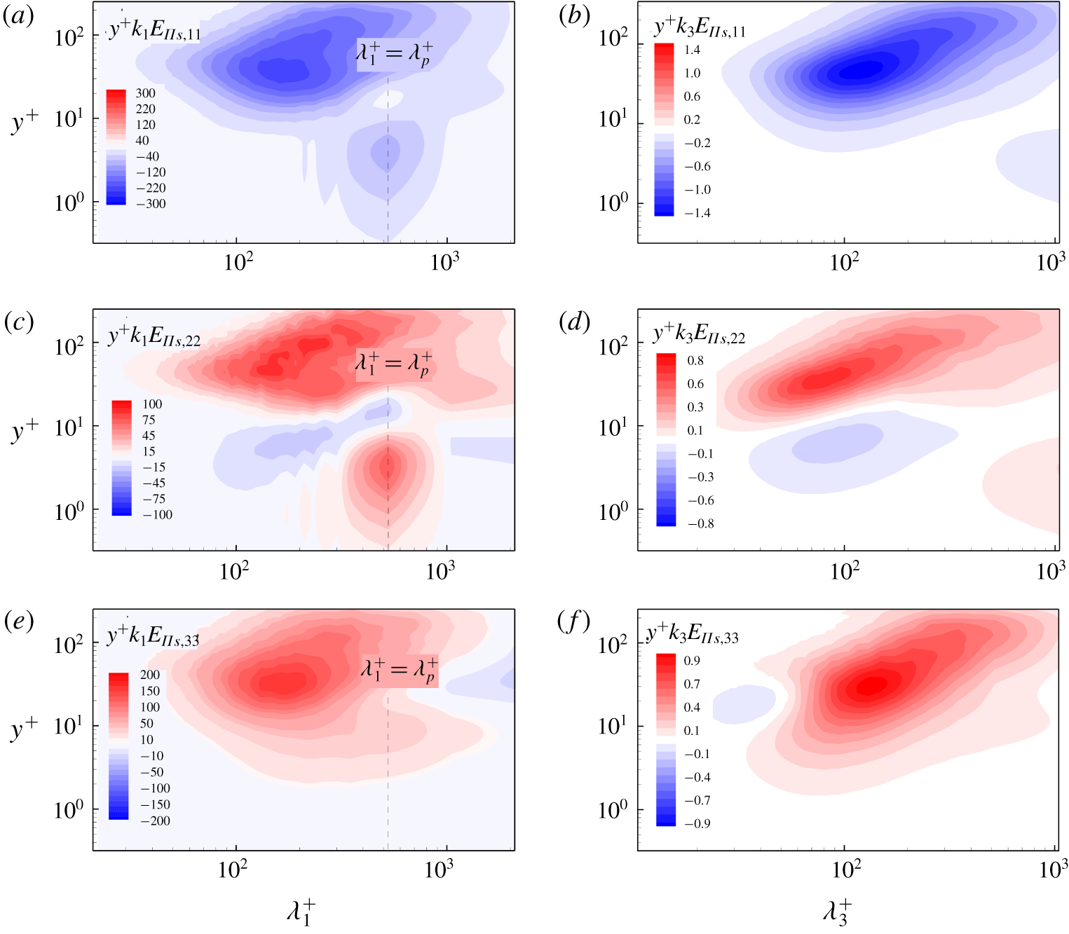
which indicates the energy transfer among different velocity components. For the flat-wall case, the one-dimensional premultiplied spectra of the pressure-strain terms are shown in figure 7. In general, the energy is transferred from the streamwise velocity component to the vertical and spanwise velocity components at  $y^{+}>10$. Figure 7(c–f) shows that at
 $y^{+}<10$, the energy near the peak region of
 $\unicode[STIX]{x1D706}_{1}^{+}=305.3$ and
 $\unicode[STIX]{x1D706}_{3}^{+}=93.6$ is transferred from the vertical component to the spanwise component, which is consistent with the result of Lee & Moser (Reference Lee and Moser2015). In addition, figure 7(f) shows that the energy of the spanwise component near
 $\unicode[STIX]{x1D706}_{3}^{+}=37.3$ is transferred to the vertical component at
 $y^{+}\approx 21.4$. This can be understood in terms of the cross-sectional flow induced by the streamwise vortices, which leads to the preferential transfer of energy into the vertical velocity fluctuations.
The  $y$- and
 $k$-premultiplied one-dimensional streamwise (a,c,e) and spanwise (b,d,f) spectra of the pressure-strain terms of different velocity components for the case of
 $c_{p}/u_{\ast }=2$: (a,b)
 $E_{\unicode[STIX]{x1D6F1}_{s},11}$; (c,d)
 $E_{\unicode[STIX]{x1D6F1}_{s},22}$; (e,f)
 $E_{\unicode[STIX]{x1D6F1}_{s},33}$.

The  $y$- and
 $k$-premultiplied one-dimensional streamwise (a,c,e) and spanwise (b,d,f) spectra of the pressure-strain terms of different velocity components for the case of
 $c_{p}/u_{\ast }=25$: (a,b)
 $E_{\unicode[STIX]{x1D6F1}_{s},11}$; (c,d)
 $E_{\unicode[STIX]{x1D6F1}_{s},22}$; (e,f)
 $E_{\unicode[STIX]{x1D6F1}_{s},33}$.

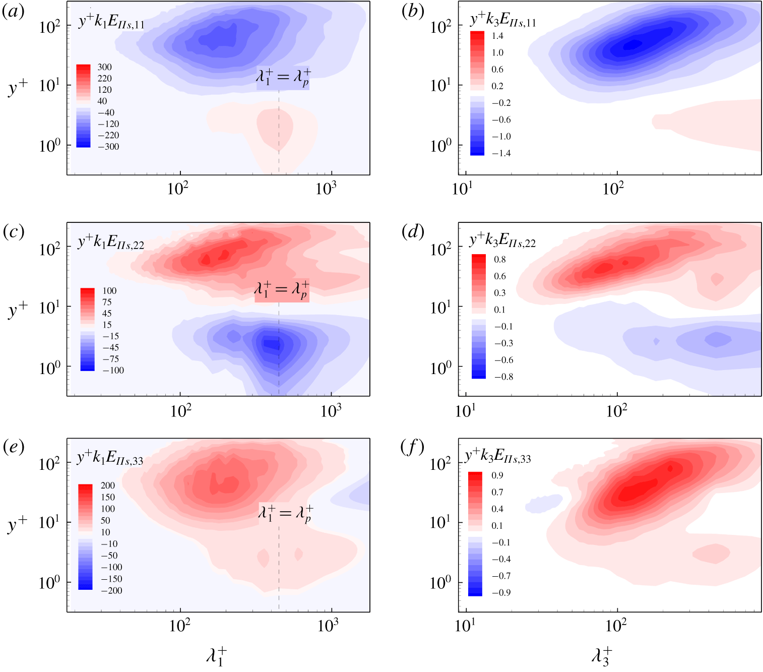
Figure 8 shows the streamwise and spanwise spectra of the pressure-strain terms for the slow-wave-field case  $c_{p}/u_{\ast }=2$. It is seen that the spectra of the pressure-strain terms are significantly affected by the surface waves. As plotted in figure 8(a,b), the energy is transferred from the streamwise component to the vertical component at the dominant wavelength scale in the region of
 $y^{+}<10$. Also, the streamwise component has a negative spanwise large-scale peak in figure 8(b), and the vertical component in figure 8(d) has a corresponding positive region. Moreover, it is noted that there is a small negative region at the dominant wavelength scale near
 $y^{+}\approx 15$ in figure 8(c), which is explained below. Moreover, the spanwise component shown in figures 8(e) and 8(f) is similar to that of the flat-wall case (figures 7e and 7f). It is noted that the spectral peak in the region of
 $y^{+}<10$ in figure 8(e) is around the dominant wavelength, although not as obvious as those in figures 8(a) and 8(c). Due to the fact that the surface waves contribute to the total energy mainly through the vertical momentum flux
 $-u^{\prime }v^{\prime }$, the energy transfer between streamwise and vertical components dominates the inter-component energy transfer. Therefore, the peaks in the spectra of the spanwise component (figure 8e,f) are much weaker and similar to those in the flat-wall case (figure 7e,f), especially in the spanwise spectra (figure 8f).
For the fast-wave-field case  $c_{p}/u_{\ast }=25$, the streamwise and spanwise spectra of the pressure-strain terms in figure 9 show apparent differences compared with the slow-wave-field case
 $c_{p}/u_{\ast }=2$ plotted in figure 8. As seen in figures 9(c) and 9(d), energy is transferred from the vertical velocity component to the other two velocity components at the dominant wavelength scale for
 $y^{+}<10$. Correspondingly, figure 9(a,b,e,f) has a positive region representing energy gain from the vertical component. The energy transfer direction among the three velocity components is opposite to the case of
 $c_{p}/u_{\ast }=2$, which is consistent with the variation of the form drag with the wave age (Sullivan et al. Reference Sullivan, McWilliams and Moeng2000; Shen et al. Reference Shen, Zhang, Yue and Triantafyllou2003; Yang & Shen Reference Yang and Shen2010). With the wave age increasing, the form drag changes from positive to negative and acts as a thrust force, which works positively on the turbulent flow. In other words, the energy is transferred from the surface waves to the overlying airflow mainly through the vertical velocity component. Subsequently, energy is transferred outwards from the vertical velocity component via the pressure-strain terms in the vicinity of the wave surface.
To explain the variation of  $E_{\unicode[STIX]{x1D6F1}_{s},22}$ along the
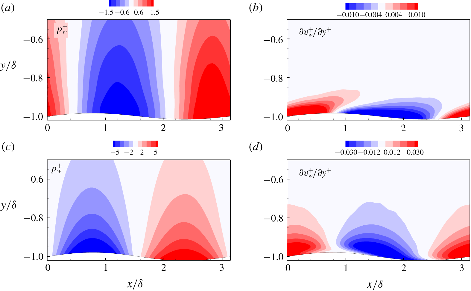
 $y$ direction at the dominant wavelength scale (figures 8c and 9c), we plot the dominant wave-induced pressure and velocity gradient fluctuations in figure 10. For the slow-wave case
 $c_{p}/u_{\ast }=2$ (figure 10a), the wave-induced pressure is in general positive on the windward side and negative on the leeward side. However, the positive (negative) region of the velocity gradient fluctuation is inclined from the windward (leeward) side to the leeward (windward) side as
 $y$ increases, as seen in figure 10(b). Since the pressure-strain terms represent the combined effect of pressure and velocity gradients (2.19),
 $E_{\unicode[STIX]{x1D6F1}_{s},22}$ at the dominant wavelength scale changes its sign from positive to negative at
 $y^{+}=10$ in figure 8(c). On the other hand, for the fast-wave case
 $c_{p}/u_{\ast }=25$, due to the rapid propagation of the surface waves, the negative and positive peaks of the velocity gradient fluctuation are twisted significantly to the upstream direction as
 $y$ increases (figure 10d). The wave-induced pressure is positive (negative) above the trough (crest) and varies only slightly in the
 $y$ direction. As a result, the variation of
 $E_{\unicode[STIX]{x1D6F1}_{s},22}$ in the
 $y$ direction of the
 $c_{p}/u_{\ast }=25$ case (figure 9c) is opposite to that of
 $c_{p}/u_{\ast }=2$ (figure 8c).
The pressure-strain term  $E_{\unicode[STIX]{x1D6F1}_{s}}$ is closely related to the net energy transfer from the wind to the surface waves. We further examine the wave growth rate based on the present simulations and compare the results with the growth rate values predicted from rapid distortion theory (Belcher & Hunt Reference Belcher and Hunt1993) and measurement data (Mastenbroek et al. Reference Mastenbroek, Makin, Garat and Giovanangeli1996; Grare et al. Reference Grare, Lenain and Melville2013) as well as numerical data (Sullivan et al. Reference Sullivan, McWilliams and Moeng2000; Liu et al. Reference Liu, Yang, Guo and Shen2010; Yang & Shen Reference Yang and Shen2010). Here we extract the dominant wave mode and the corresponding pressure at the surface to compute the wave growth rate
 $\unicode[STIX]{x1D6FD}$ following Liu et al. (Reference Liu, Yang, Guo and Shen2010). Suppose the dominant wave component of the surface elevation is
 $\unicode[STIX]{x1D702}(x,t)=a\cos (k_{p}x-\unicode[STIX]{x1D714}_{p}t)$ and the corresponding surface pressure is
 $p(x,t)=\unicode[STIX]{x1D6FC}ak\cos (k_{p}x-\unicode[STIX]{x1D714}_{p}t+\unicode[STIX]{x1D703})$, where
 $\unicode[STIX]{x1D6FC}$ denotes the amplitude ratio of the pressure to the wave steepness and
 $\unicode[STIX]{x1D703}$ denotes the phase difference between the pressure and the waveform. The wave growth rate is then obtained as:
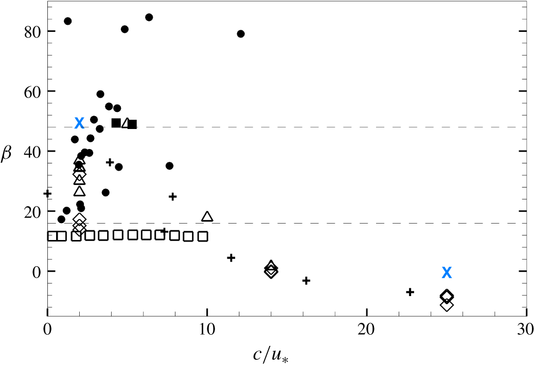
 $\unicode[STIX]{x1D6FD}=(\unicode[STIX]{x1D6FC}\sin \unicode[STIX]{x1D703})/\unicode[STIX]{x1D70C}u_{\ast }^{2}$. In general, the results are consistent. For the slow-wave-field case, the current result is close to the measurements completed in wave tanks (Mastenbroek et al. Reference Mastenbroek, Makin, Garat and Giovanangeli1996; Grare et al. Reference Grare, Lenain and Melville2013) as shown in figure 11, which are larger than the theoretical predictions obtained by Belcher & Hunt (Reference Belcher and Hunt1993). Note that the wave steepness also affects the wave growth rate. Therefore, even when the wave age is fixed, there is a noticeable scattering in the wave growth rates calculated in different experimental and numerical studies (e.g. see the data near
 $c/u_{\ast }=2$ in figure 11).
Dominant wave-induced pressure (a,c) and velocity gradient (b,d) fluctuations: (a,b)  $c_{p}/u_{\ast }=2$; (c,d)
 $c_{p}/u_{\ast }=25$.

Wave growth rate  $\unicode[STIX]{x1D6FD}$ as a function of wave age
 $c/u_{\ast }$. Wave tank measurement data are denoted by: ▪, Mastenbroek et al. (Reference Mastenbroek, Makin, Garat and Giovanangeli1996); ●, Grare et al. (Reference Grare, Lenain and Melville2013). Previous numerical results are denoted by:
 $+$, Sullivan et al. (Reference Sullivan, McWilliams and Moeng2000); ▵, Liu et al. (Reference Liu, Yang, Guo and Shen2010); ♢, Yang & Shen (Reference Yang and Shen2010). Also plotted are the upper (
 $\unicode[STIX]{x1D6FD}=48$) and lower (
 $\unicode[STIX]{x1D6FD}=16$) limits of the observation-based empirical formula of Plant (Reference Plant1982), denoted by the horizontal dashed lines. The wave growth rates obtained with the analytical theory of Belcher & Hunt (Reference Belcher and Hunt1993) are denoted by ▫. Present simulation results are denoted by
 $\times$.

The above results of energy transfer among different velocity components are summarized as follows. For flat-wall turbulence, the energy is transferred from the streamwise component to the other two components via the pressure-strain terms in the region of  $y^{+}>10$. In the presence of surface waves, additional inter-component energy transfer occurs at the dominant wavelength scale in the near-surface region. For the slow-wave case
 $c_{p}/u_{\ast }=2$, the inter-component energy transfer direction at the dominant wavelength scale at
 $y^{+}<10$ is consistent with the main transfer direction in flat-wall turbulence. On the contrary, the energy at the dominant wavelength scale is transferred from the vertical component to the other two components at
 $y^{+}<10$ for the fast-wave case
 $c_{p}/u_{\ast }=25$.
The  $y$- and
 $k$-premultiplied one-dimensional streamwise spectra of the turbulent kinetic energy: (a,d,g) viscous transport, (b,e,h) pressure transport and (c,f,i) spatial turbulent transport, in the cases of (a–c) flat wall; (d–f)
 $c_{p}/u_{\ast }=2$; (g–i)
 $c_{p}/u_{\ast }=25$.

3.5 Spatial energy transport
In the region where the energy production from the mean shear is high, the energy is transported vertically to the regions above and below it. As discussed in § 2.3, there are three mechanisms in the spatial energy transport process, namely the viscous transport  $T_{v,ij}$, the pressure transport
 $T_{p,ij}$ and the spatial turbulent transport
 $T_{t,ij}^{\unicode[STIX]{x1D6FC}}$.
The premultiplied one-dimensional streamwise spectra of the turbulent kinetic energy spatial transport terms are plotted in figure 12. In general, the effect of the viscous transport is confined to the region of  $y^{+}<70$. For the flat-wall case, it is seen in figure 12(a) that energy is transferred from the buffer region to the very-near-wall region and the outer region through the viscous transport. The negative peak in figure 12(a) is close to the positive peak of the production term in figure 5(a), where the turbulent energy is the highest and is thus transferred to other regions. For the case of
 $c_{p}/u_{\ast }=2$, the energy transfer is also from the buffer region to the near-surface and outer regions except that the streamwise length scale of the peak region changes to the dominant wavelength (figure 12d). As the wave age increases to
 $c_{p}/u_{\ast }=25$, the energy transfer to the very-near-surface region via the viscous transport (red region) increases and occurs at the dominant wavelength scale (figure 12g).
As for the turbulent kinetic energy pressure transport, it contributes the least to the spatial energy flux in the flat-wall case as compared with the other two energy transport terms. As shown in figure 12(b), the energy transport direction is consistent with the viscous term, but its effect does not reach the surface. In the presence of surface waves, the direction of the pressure transport is strongly dependent on the wave age. For the case of  $c_{p}/u_{\ast }=2$, the energy is transferred from the very-near-surface region to the buffer region at the dominant wavelength scale as seen in figure 12(e), while the energy is transferred from the buffer region to the very-near-surface region in the case of
 $c_{p}/u_{\ast }=25$ (figure 12h). The opposite direction of the turbulent energy transport by pressure can also be explained by the difference in the form drag at different wave ages. As shown in Sullivan et al. (Reference Sullivan, McWilliams and Moeng2000) and Yang & Shen (Reference Yang and Shen2010), the air pressure distribution near the wall is significantly affected by the wave age. When the wave age increases to the fast-wave range, the form drag becomes negative and acts as a thrust, leading to a significant difference in the pressure–velocity correlation.
After decomposing  $T_{t,ij}$ into
 $T_{t,ij}^{\unicode[STIX]{x1D6FC}}$ and
 $T_{t,ij}^{\unicode[STIX]{x1D6FD}}$ as in (2.25), the spectrum of
 $T_{t,ij}^{\unicode[STIX]{x1D6FC}}$ can be interpreted as the spatial turbulent transport in the vertical direction. For the flat-wall case, this term contributes the most to the total energy spatial transport as shown in figure 12(c). Moreover, the spatial turbulent transport can affect higher locations as compared with the viscous transport in figure 12(a). For the case of
 $c_{p}/u_{\ast }=2$, the energy transfer through spatial turbulent transport increases and the spectral peak as seen in figure 12(f) changes to the dominant wavelength. For the case of
 $c_{p}/u_{\ast }=25$, due to the fact that the surface waves provide additional energy generation from the mean shear, there is another negative area in the very-near-surface region at the dominant wavelength scale, where the energy is transported outwards via
 $T_{t,ij}^{\unicode[STIX]{x1D6FC}}$ as seen in figure 12(i).
In summary, among the three types of spatial energy transport mechanisms, turbulent energy is transported to the near-surface region by viscous and turbulent transport terms at the dominant wavelength scale for both the slow- and fast-wave cases. Interestingly, the pressure transport direction at the dominant wavelength scale is reversed as the wave age increases, consistent with the opposite near-surface pressure distributions between figures 10(a) and 10(c).
3.6 Inter-scale energy transfer
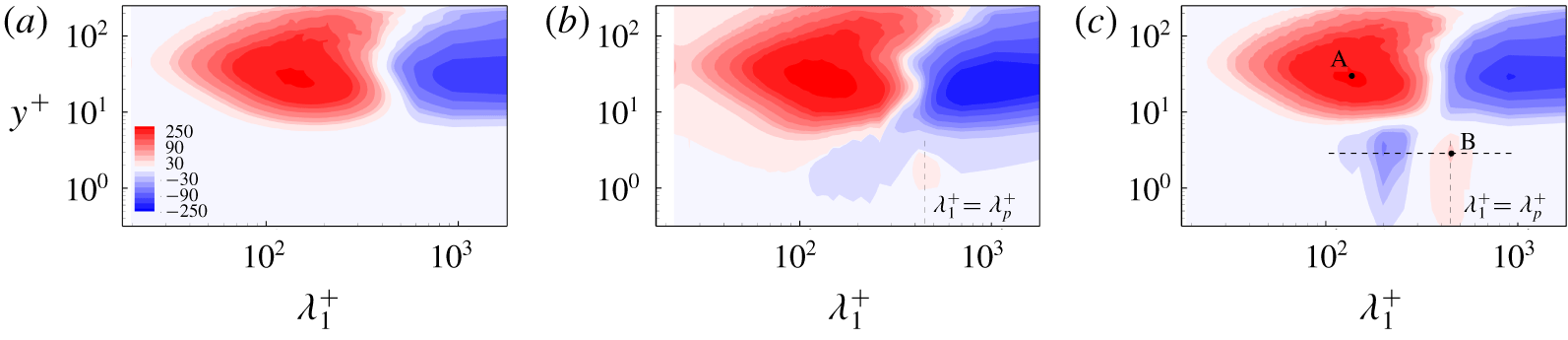
In addition to the energy transport in the physical space discussed in § 3.5, the energy transfer in the spectral space is also of great importance due to its relation to the energy cascade process, and is discussed in this subsection. Figure 13 shows the premultiplied one-dimensional streamwise spectra of the inter-scale energy transport term in (2.32),  $E_{T_{t}^{\unicode[STIX]{x1D6FD}},11}$. For the flat-wall case,
 $E_{T_{t}^{\unicode[STIX]{x1D6FD}},11}$ in figure 13(a) shows that the energy-containing large-scale streamwise motion transfers energy to the small-scale motion at
 $y^{+}>10$, corresponding to the well-known energy cascade process. In the presence of surface waves, it is interesting that the energy of the small-scale streamwise motions is transferred backward to the dominant wavelength scale at
 $y^{+}<5$ as seen in figure 13(b). As the wave age increases to
 $c_{p}/u_{\ast }=25$, the inverse cascade in the near-surface region becomes more obvious (figure 13c). Because the direction of the inter-scale energy transfer does not change with the wave age, the case of
 $c_{p}/u_{\ast }=25$ and the flat-wall case are chosen to illustrate the surface wave effect further.
The  $y$- and
 $k$-premultiplied one-dimensional streamwise spectra of the inter-scale energy transport term,
 $E_{T_{t}^{\unicode[STIX]{x1D6FD}},11}$: (a) the flat-wall case; (b)
 $c_{p}/u_{\ast }=2$; (c)
 $c_{p}/u_{\ast }=25$.

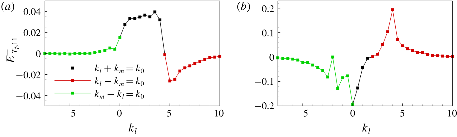
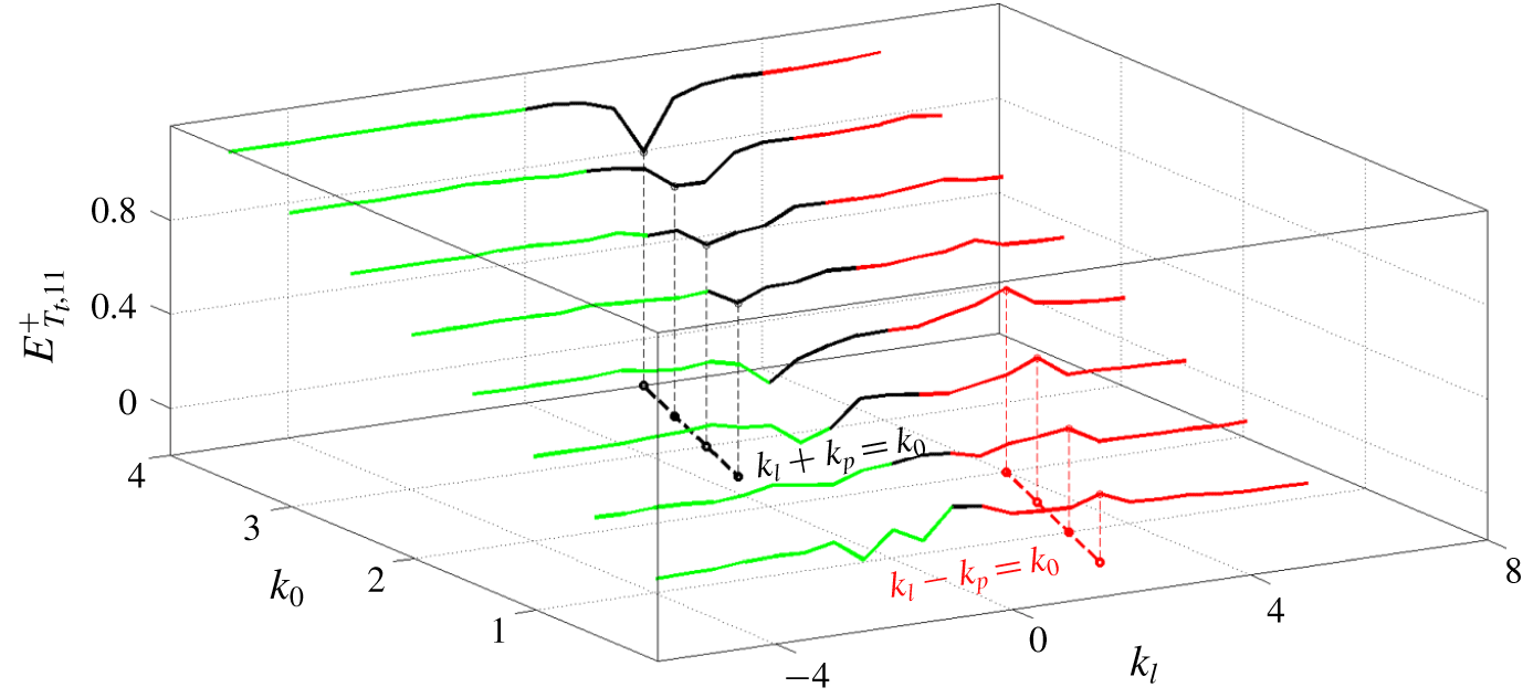
Considering that the inter-scale energy transport process is complex and features nonlinearity, we resort to triadic interactions at a given wavenumber  $k_{0}$ to investigate the underlying mechanism. The wavenumbers
 $k_{l}$ and
 $k_{m}$ satisfying the triadic relationships
 $k_{l}+k_{m}=k_{0}$ lead to excitation at
 $k_{0}$. The one-dimensional spectrum of the turbulent transport term is rewritten as discretized convolution (Cho et al. Reference Cho, Hwang and Choi2018):
 $$\begin{eqnarray}E_{T_{t},ij}(k_{0},y)=\left\langle Re\left\{-\overline{\hat{u} _{i}^{\prime \ast }(k_{0},y)\frac{\unicode[STIX]{x2202}}{\unicode[STIX]{x2202}x_{j}}\mathop{\sum }_{k_{l}+k_{m}=k_{0}}\hat{u} _{i}^{\prime }(k_{l},y)\hat{u} _{j}^{\prime }(k_{m},y)}\right\}\right\rangle _{z},\end{eqnarray}$$
where  $k_{l}$ and
 $k_{m}$ are the streamwise wavenumbers. In the analysis of Cho et al. (Reference Cho, Hwang and Choi2018), they focused on the triadic interactions in the spanwise direction. Because in the present problem there exists a characteristic length scale in the streamwise direction associated with the dominant wave and thus a peak in the streamwise spectrum in the near-surface region as shown in figures 13(b) and 13(c), we choose the streamwise triadic interactions to explore the inter-scale energy transfer. For a positive
 $k_{0}$, the convolution in (3.2) can be written as
 $$\begin{eqnarray}\displaystyle \mathop{\sum }_{k_{l}+k_{m}=k_{0}}\hat{u} _{i}^{\prime }(k_{l})\hat{u} _{j}^{\prime }(k_{m}) & = & \displaystyle \mathop{\sum }_{\substack{ k_{l}+k_{m}=k_{0} \\ k_{l},k_{m}\geqslant 0}}\hat{u} _{i}^{\prime }(k_{l})\hat{u} _{j}^{\prime }(k_{m})\nonumber\\ \displaystyle & & \displaystyle +\,\mathop{\sum }_{\substack{ k_{m}-k_{l}=k_{0} \\ k_{l},k_{m}\geqslant 0}}\hat{u} _{i}^{\prime }(-k_{l})\hat{u} _{j}^{\prime }(k_{m})+\mathop{\sum }_{\substack{ k_{l}-k_{m}=k_{0} \\ k_{l},k_{m}\geqslant 0}}\hat{u} _{i}^{\prime }(k_{l})\hat{u} _{j}^{\prime }(-k_{m}).\end{eqnarray}$$
Two distinct positive spectral peaks in figure 13(c) (marked as points A and B) are chosen as the given streamwise wavenumbers and vertical locations. Figure 14 shows the inter-scale energy transported to the wavenumber  $k_{0}$ via triadic interactions at the corresponding points A and B. For point A, where the corresponding streamwise wavenumber is
 $k_{0}=4.5$, the positive turbulent energy transport is dominated by the interactions in the region of
 $k_{l}+k_{m}=k_{0}$ as shown in figure 14(a). This indicates that the energy influx to the motion at the given wavenumber
 $k_{0}$ is mainly from the eddies with larger streamwise sizes, in accordance with the streamwise spectrum of
 $E_{T_{t}^{\unicode[STIX]{x1D6FD}},11}$ as shown in figure 13(c). The related energy cascade is consistent with the result of Cho et al. (Reference Cho, Hwang and Choi2018). For point B in the near-surface region, the energy peak corresponds to the dominant surface wave
 $k_{0}=k_{p}=2$. Although point B has the maximum turbulent energy influx in the near-surface region, the corresponding triadic interactions as plotted in figure 14(b) are quite different from those of point A. In the vicinity of the surface, the triadic interactions leading to the positive turbulent transport mainly occur in the region of
 $k_{l}-k_{m}>k_{0}$, indicating that the energy influx at the dominant wavenumber is mediated by the triadic interactions between the turbulent motions that have smaller streamwise sizes than the given one. In addition, the positive peak in figure 14(b) corresponds to the second harmonic wavenumber
 $k_{l}=2k_{p}=4$. This peak is in accordance with the negative peak in the near-surface region (see figure 13c), indicating the second harmonic wave contributes most to the energy influx at
 $k_{p}$.
Inter-scale turbulent energy transport via triadic interactions at points A (a) and B (b) marked in figure 13(c) for the case of  $c_{p}/u_{\ast }=25$.

Inter-scale turbulent energy transport via triadic interactions along the dashed line marked in figure 13(c). The green, black and red lines denote the triadic relationships  $-k_{l}+k_{m}=k_{0}$,
 $k_{l}+k_{m}=k_{0}$ and
 $k_{l}-k_{m}=k_{0}$, respectively. Note that
 $k_{m}=k_{p}$ on the black and red dashed lines. The value of
 $k_{0}$ ranges from 0.5 to 4.0 with an interval of 0.5. For clarity, each successive interaction curve is raised by 0.15 above the preceding curve at a lower
 $k_{0}$.

Next, we take a closer look at the horizontal dashed line in figure 13(c), which is at the vertical location of point B. The triadic interactions along this line are expected to explain the inverse energy cascade in the near-surface region discussed above. Figure 15 shows the triadic interactions for different values of  $k_{0}$ along the dashed line in figure 13(c). The value of
 $k_{0}$ ranges from 0.5 to 4.0, with an interval of 0.5. Given the streamwise wavenumber
 $k_{0}$, the energy transfer only occurs between pairs of wavenumbers that satisfy the triadic interactions in (3.3). A distinct trough and peak can be observed from figure 15. The corresponding wavenumber pairs
 $(k_{0},k_{l})$ are indicated by the black dashed line and red dashed line, respectively. At the trough (black dashed line in figure 15), all the wavenumber pairs
 $(k_{0},k_{l})$ satisfy the triadic relationship
 $k_{l}+k_{m}=k_{0}$ (
 $k_{m}=k_{p}$ here), indicating that the motions of higher wavenumbers
 $k_{0}>k_{p}$ transfer energy to the dominant wavenumber
 $k_{p}$. For a given streamwise wavenumber
 $k_{0}\leqslant k_{p}=2$, a positive peak occurs at
 $k_{l}$ satisfying the triadic relationship
 $k_{l}-k_{m}=k_{0}$ (
 $k_{m}=k_{p}$ here), denoted as the red dashed line in figure 15. This suggests that the energy influx to the given streamwise wavenumber
 $k_{0}$ is caused by the scale interactions between the dominant wavenumber
 $k_{p}$ and
 $k_{l}>k_{0}$. Note that
 $E_{T_{t}^{\unicode[STIX]{x1D6FD}},11}$ in figure 14(b) is positive as
 $k_{l}$ varies from 2.5 to 4.0, indicating that these small-scale motions at
 $k_{l}$ transfer energy to the dominant wavelength
 $k_{p}$, consistent with the trough in figure 15. In addition to the inter-scale energy transfer related to the dominant wavelength scale of broadband waves, it should be mentioned that relatively weak energy transfer among other scales also exists.
As a summary, the energy transport process including the spatial and inter-scale energy transports is sketched in figure 16. In general, energy is transported from the buffer region to the very-near-surface and outer regions. In the average sense, large-scale motions transfer energy to small-scale motions via  $T_{t}^{\unicode[STIX]{x1D6FD}}$ above the buffer region. In the presence of surface waves, energy transport to the near-surface region via spatial viscous and turbulent transport terms occurs at the dominant wavelength scale for both the slow and fast wave fields, while the pressure transport direction at the dominant wavelength scale changes sign for different wave ages. In the slow-wave case, the energy is transported outwards from the region of
 $y^{+}<5$ (denoted as red solid arrows), and the opposite process occurs in the fast-wave case (denoted as red dashed arrows). Moreover, energy of small-scale motions is transferred to the dominant wavelength scale via inter-scale transport in the vicinity of the surface.
Schematic of the spatial and inter-scale energy transfer process in the presence of surface waves. The spiral symbols represent the turbulent motions of different length scales above the buffer region, and the wavy symbols represent the turbulent motions of different length scales in the very vicinity of surface waves. The black solid arrows denote the energy transfer directions in the flat-wall case. The red solid (dashed) arrows denote the directions of the newly emerging energy transfer in the slow (fast) wave field case.

4 Conclusions
In this study, DNS is performed for turbulent flow over surface waves, with the dynamics of the surface waves captured by the HOS method. The initial wave field is given by a broadband wave spectrum, and the effect of the waves on the energy transfer in the overlying turbulent flow is examined. For the slow-wave case of  $c_{p}/u_{\ast }=2$, the dominant wave and its harmonics contribute the most to the energy spectrum in the buffer region, and the original streaky structures are disrupted by the surface waves. In the fast-wave case of
 $c_{p}/u_{\ast }=25$, the energy spectrum protrudes from the surface over a wide range of length scales due to the direct contribution of surface waves to the total kinetic energy. As the distance from the wavy surface increases, the wave effect on the energy distribution in the buffer region is greatly attenuated, and the corresponding flow pattern resembles that of flat-wall turbulence.
We have, for the first time, performed a spectral analysis of the two-point correlation transport equation to elucidate the turbulent energy transfer process in the presence of surface waves. Due to the wave motion, the production term has an additional peak in the near-surface region of  $y^{+}<20$ as compared with the flat-wall case. Among the transport terms, the effect of viscous transport is confined to the region of
 $y^{+}<70$, and the process of energy transport from the buffer region to the very-near-surface region at the dominant wavelength scale is enhanced. The turbulent transport contributes the most to the spatial energy transport and affects higher altitudes. Moreover, an additional negative turbulent transport region appears at the dominant wavelength scale in the fast-wave-field case. We have also shown that the pressure-related turbulent energy transfer is dependent on the wave age. For the pressure diffusion term, the energy at the dominant wavelength scale in the region of
 $y^{+}<10$ is transferred outwards in the slow-wave case of
 $c_{p}/u_{\ast }=2$, while the energy in the buffer region is transferred to the near-surface region in the fast-wave case of
 $c_{p}/u_{\ast }=25$. For the inter-component energy transfer through the pressure-strain term, the energy is transferred from the streamwise component to the vertical component at the dominant wavelength scale in the region of
 $y^{+}<10$ in the
 $c_{p}/u_{\ast }=2$ case, while the energy is transferred from the vertical component to the other two components in the
 $c_{p}/u_{\ast }=25$ case. The other part of the nonlinear term, i.e. the inter-scale transport term, transfers energy among different length scales. In general, the large-scale energy-containing motions transfer energy to small-scale motions via the inter-scale transport term, which corresponds to the well-known energy cascade process. Conversely, in the presence of surface waves, energy is transferred from small-scale motions to the turbulent motion at the dominant wavenumber in the very-near-surface region. From the triadic interactions at a given streamwise wavenumber, it is found that the energy influx at the dominant wavelength scale is mainly due to the contribution of the adjacent streamwise wavenumbers, and the turbulent motions at the second harmonic wavenumber contribute the most. In addition to the spectral peak at the dominant wavenumber similar to the monochromatic wave case, the instantaneous field and inter-scale energy transfer also reflect the contributions from the broadband wave components.
The physical picture revealed in this DNS-based, mechanistic study regarding wave effects on the energy transfer process among different length scales in spectral space and different vertical locations in physical space serves as an important first step towards improved modelling for air–sea interactions, e.g. the subgrid-scale modelling of turbulent airflows overlying waves that critically relies on a fundamental understanding of the energy transfer process. Extending the computational framework to more complex cases and developing turbulence models for air–sea interaction applications are beyond the scope of this study, but should be considered in future research.
Acknowledgements
L.-H.W., W.-Y.Z., W.-X.H., C.-X.X. and Z.Z. acknowledge the support of the National Natural Science Foundation of China under grants nos. 11772172, 91752205 and 11490551 and the parallel computing resources provided by Tsinghua National Laboratory for Information Science and Technology. X.H. and L.S. gratefully acknowledge the support of the National Science Foundation and Minnesota Sea Grant. The authors also thank the anonymous reviewers for their valuable comments.
Declaration of interests
The authors report no conflict of interest.
Appendix A. Property of inter-scale turbulent transport
In the spectral analysis of the budget equation (2.17) in wall-bounded turbulent flows, there are multiple ways to decompose the nonlinear turbulent term into spatial and inter-scale parts. In the present study, the decomposition (2.25) is consistent with the definitions used by Mizuno (Reference Mizuno2016) and Lee & Moser (Reference Lee and Moser2019). In curvilinear coordinates, when  $r_{\unicode[STIX]{x1D709}_{1}}=r_{\unicode[STIX]{x1D709}_{3}}=0$, the inter-scale turbulent transport term (2.27) satisfies
 $$\begin{eqnarray}\displaystyle T_{t,ij}^{\unicode[STIX]{x1D6FD}} & = & \displaystyle -\overline{u_{j}^{\prime }\frac{\unicode[STIX]{x2202}u_{i}^{\prime }u^{\prime }}{\unicode[STIX]{x2202}\unicode[STIX]{x1D709}_{1}}}-\overline{u_{i}^{\prime }\frac{\unicode[STIX]{x2202}u_{j}u^{\prime }}{\unicode[STIX]{x2202}\unicode[STIX]{x1D709}_{1}}}-\overline{u_{j}^{\prime }\frac{\unicode[STIX]{x2202}u_{i}^{\prime }w^{\prime }}{\unicode[STIX]{x2202}\unicode[STIX]{x1D709}_{3}}}-\overline{u_{i}^{\prime }\frac{\unicode[STIX]{x2202}u_{j}^{\prime }w^{\prime }}{\unicode[STIX]{x2202}\unicode[STIX]{x1D709}_{3}}}\nonumber\\ \displaystyle & & \displaystyle -\,\frac{\unicode[STIX]{x2202}\overline{u_{i}^{\prime }u_{j}^{\prime }v^{\prime }}}{\unicode[STIX]{x2202}\unicode[STIX]{x1D709}_{2}}+\overline{v^{\prime }\frac{\unicode[STIX]{x2202}u_{i}^{\prime }u_{j}^{\prime }}{\unicode[STIX]{x2202}\unicode[STIX]{x1D709}_{2}}}-\overline{\unicode[STIX]{x1D719}_{k}\frac{\unicode[STIX]{x2202}u_{i}^{\prime }u_{j}^{\prime }u_{k}^{\prime }}{\unicode[STIX]{x2202}\unicode[STIX]{x1D709}_{2}}}+\overline{u_{k}^{\prime }\unicode[STIX]{x1D719}_{k}\frac{\unicode[STIX]{x2202}u_{i}^{\prime }u_{j}^{\prime }}{\unicode[STIX]{x2202}\unicode[STIX]{x1D709}_{2}}}.\end{eqnarray}$$
By making use of the chain rule of partial differential (2.6) and the continuity,
 $$\begin{eqnarray}T_{t,ij}^{\unicode[STIX]{x1D6FD}}=-\overline{u_{i}^{\prime }u_{j}^{\prime }\frac{\unicode[STIX]{x2202}u_{k}^{\prime }}{\unicode[STIX]{x2202}\unicode[STIX]{x1D709}_{k}}}-\overline{\frac{\unicode[STIX]{x2202}u^{\prime }u_{i}^{\prime }u_{j}^{\prime }}{\unicode[STIX]{x2202}\unicode[STIX]{x1D709}_{1}}\text{ + }\frac{\unicode[STIX]{x2202}w^{\prime }u_{i}^{\prime }u_{j}^{\prime }}{\unicode[STIX]{x2202}\unicode[STIX]{x1D709}_{3}}}-\overline{\unicode[STIX]{x1D719}_{k}u_{i}^{\prime }u_{j}^{\prime }\frac{\unicode[STIX]{x2202}u_{k}^{\prime }}{\unicode[STIX]{x2202}\unicode[STIX]{x1D709}_{2}}}=0.\end{eqnarray}$$
Hence, the two-dimensional spectrum  $E_{T_{t}^{\unicode[STIX]{x1D6FD}},ij}$, i.e. the Fourier transform of
 $T_{t,ij}^{\unicode[STIX]{x1D6FD}}$, inherits the property and satisfies
 $$\begin{eqnarray}\int \!\int _{0}^{\infty }E_{T_{t}^{\unicode[STIX]{x1D6FD}},ij}(k_{1},\unicode[STIX]{x1D709}_{2},k_{3})\,\text{d}k_{1}\,\text{d}k_{3}=0,\quad \forall \unicode[STIX]{x1D709}_{2}.\end{eqnarray}$$
We can therefore interpret  $T_{t,ij}^{\unicode[STIX]{x1D6FD}}$ as the inter-scale energy transfer.