Implications

Dispersion-specific differential gene expression across physiological stages has been evaluated on ovary, uterus and hypophysis from 22 F₂ Iberian × Meishan sows. The heteroskedastic model evidenced relevant departures of the residual variance in 2.9% to 37.4% of the analyzed probes, highlighting a remarkable incidence of this phenomenon in pigs. Moreover, scale-effect disturbances were discarded in most of the probes with dispersion-specific differential gene expression. These results provided the first evidence of heteroskedasticity for gene expression in a livestock species, suggesting the possibility of dispersion-related regulatory genetic mechanisms involved in sow reproduction.

Material and methods

This research was carried out on frozen tissues and live animals were not required. Nevertheless, all animal protocols regarding the original F₂ Iberian × Meishan sows were approved by the Institut de Recerca i Tecnologia Agroalimentàries (IRTA; http://www.irta.cat) Animal Care and Use committee within the context of research project AGL2000-1229-C03.

Tissue collection

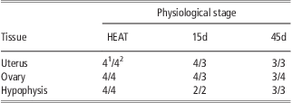
A total of 61 tissue samples from ovary, uterus and hypophysis of 22 F₂ Iberian × Meishan sows were recovered at the commercial slaughterhouse (ESFOSA, Vic, Spain). More specifically, both the whole hypophysis and one ovary were collected when possible, whereas a sample from the apical uterus was obtained close to the oviduct. Samples were immediately frozen in liquid nitrogen and stored at −80°C until laboratory processing. All sows were in their fifth gestation (i.e. they had delivered four times), although they were slaughtered at different reproductive stages: heat (HEAT; n = 8), 15 days of pregnancy (15d; n = 7) and 45 days of pregnancy (45d; n = 7). Note that pregnancies were confirmed before slaughtering by ultrasound. Moreover, sows contributing to this experiment were selected depending on their reproductive performance in order to generate two groups with extreme prolificacy histories measured as the total number of piglets born per litter, that is, low average litter size (L; 5.78 ± 2.53 piglets per litter) and high average litter size (H; 11.48 ± 1.47 piglets per litter). A summary of the number of tissue samples per reproductive stage and performance is shown in Table 1.

Table 1

Number of microarrays for each tissue and physiological stage combination

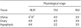
¹Microarrays from lowly prolific sows.

²Microarrays from highly prolific sows.

Heteroskedastic linear mixed model

For each pairwise comparison between two physiological stages Ω₁ and Ω₂ of a given tissue, data from n replicates of non-competitive hybridization microarrays were available. Gene expression data were analyzed under the following hierarchical mixed model:

$${\bf {{y}}}\, = \,{\bf {{X\brmu }}}\, + \,{{{\bf {{Z}}}}_1}{{{\bf {{p}}}}_1}\, + \,{{{\bf {{Z}}}}_2}{{{\bf {{p}}}}_2}\, + \,{{{\bf {{Z}}}}_3}{{{\bf {{p}}}}_3}\, + \,{{{\bf {{Z}}}}_4}{{{\bf {{p}}}}_4}\, + \,{\bf {{e}}}$$

where y was the (nm) × 1 column vector of intensity scores sorted by microarray, within treatment within probe, and e was the (nm) × 1 column vector of residuals. Preliminary analyses on this data set suggested significant differential gene expression on the basis of sow prolificacy. Within this context, sows were classified as lowly (L) or highly (H) prolific (see Table 1), and the model accounted for the interaction between sow prolificacy and physiological stage with four levels, L × Ω₁ (p₁; dimension n ₁ × 1) and H × Ω₁ (p₂; dimension n ₂ × 1), L × Ω₂ (p₃; dimension n ₃ × 1) and H × Ω₂ (p₄; dimension n ₄ × 1), where n = n ₁ + n ₂ + n ₃ + n ₄. Note that p₁ to p₄ accounted for the effect of each probe, whereas μ was a systematic effect characterizing the overall mean of each microarray, and X, Z₁, Z₂, Z₃ and Z₄ were appropriate incidence matrices.

Following Casellas and Varona (Reference Casellas and Varona2008), vector e was assumed to be normally distributed,

$${\bf e}\,\sim \,{\rm{MVN}}\left( {{\bf {{0}}},{\bf {{R}}}} \right)$$

with R being the matrix of residual (co)variances. Assuming null residual (co)variances (Kendziorski et al., Reference Kendziorski, Newton, Lan and Gould2003; Newton et al., Reference Newton, Noueiry, Sarkar and Ahlquist2004; Casellas et al., Reference Casellas, Ibáñez-Escriche, Martínez-Giner and Varona2008), heteroskedasticity between physiological stages was analyzed by stating

$${\bf {{R}}}\, = \,{\mathop{ \oplus }\limits_{{i\, = \,1}}^{m}} \left[ {<!\begin{array}{*{20}c}>\matrix{ {{{{\bf {{I}}}}_1}\sigma _{{e\left( i \right)}}^{2} {{\pi }_i}} & {\bf {{0}}} \\ {{\bf {{0^{\prime}}}}} & {{{{\bf {{I}}}}_2}\sigma _{{e\left( i \right)}}^{2} \left( {1{\rm{ - }}{{\pi }_i}} \right)} \\\end{array}}} \right]$$

where I₁ was a (n ₁ + n ₂) × (n ₁ + n ₂) identity matrix, I₂ was a (n ₃ + n ₄) × (n ₃ + n ₄) identity matrix, 0 was a (n ₁ + n ₂) × (n ₃ + n ₄) matrix of zeros, $$$\sigma _{{e\left( i \right)}}^{2} $$$ was the sum of residual variance for the ith probe in both physiological stages and π_i was the probe-specific heteroskedasticity parameter. As shown by Casellas and Varona (Reference Casellas and Varona2008), π_i = 0.5 accounted for equal residual variances between treatments and π_i ≠ 0.5 suggested within-probe (between treatments) heteroskedasticity. Given the reduced number of replicates within each physiological stage, a common residual variance was assumed for both L and H sows.

This model was analyzed under a standard Bayesian development with the following joint posterior probability:

$$\displaylines{ & p\left( {{\bf {{\brmu }}},{{{\bf {{p}}}}_1},{{{\bf {{p}}}}_2},{{{\bf {{p}}}}_3},{{{\bf {{p}}}}_4},{\bf {{\brsigma }}},{\bf {{\brpi }}},\sigma _{{p1}}^{2}, \sigma _{{p2}}^{2}, \sigma _{{p3}}^{2}, \sigma _{{p4}}^{2} \left| {\bf {{y}}} \right.} \right) \cr & \propto p\left( {{\bf {{y}}}\left| {{\bf {{a}}},{{{\bf {{p}}}}_1},{{{\bf {{p}}}}_2},{{{\bf {{p}}}}_3},{{{\bf {{p}}}}_4},{\bf {{R}}}} \right.} \right)p\left( {\bf {{\brmu }}} \right) \times p\left( {{{{\bf {{p}}}}_1}\left| {\sigma _{{p1}}^{2} } \right.} \right)p\left( {\sigma _{{p1}}^{2} } \right) \cr & p\left( {{{{\bf {{p}}}}_2}\left| {\sigma _{{p2}}^{2} } \right.} \right)p\left( {\sigma _{{p2}}^{2} } \right)p\left( {{{{\bf {{p}}}}_3}\left| {\sigma _{{p3}}^{2} } \right.} \right) p\left( {\sigma _{{p3}}^{2} } \right)p\left( {{{{\bf {{p}}}}_4}\left| {\sigma _{{p4}}^{2} } \right.} \right) \cr & p\left( {\sigma _{{p4}}^{2} } \right) \times p\left( {\bf {{\brsigma }}} \right)p\left( {\bf {{\brpi }}} \right) $$

where $$$\brsigma ^{\prime}\, = \,\left[ {<!\begin{array}{*{20}c}>\matrix{ {\sigma _{{e\left( {\rm{1}} \right)}}^{{\rm{2}}} } & {\sigma _{{e\left( {\rm{2}} \right)}}^{{\rm{2}}} } & \ldots & {\sigma _{{e\left( m \right)}}^{{\rm{2}}} } \\\end{array}}} \right],\,\,\brpi ^{\prime}\, = \,\left[ {<!\begin{array}{*{20}c}>\matrix{ {{{\pi }_1}} & {{{\pi }_2}} & \ldots & {{{\pi }_m}} \\\end{array}}} \right]$$$ and the Bayesian likelihood was stated as multivariate normal,

$$\openup 3pt{ & p\left( {{\bf {{y}}}\left| {{\bf {{\brmu }}},{{{\bf {{p}}}}_1},{{{\bf {{p}}}}_2},{{{\bf {{p}}}}_3},{{{\bf {{p}}}}_4},{\bf {{R}}}} \right.} \right)\,{\rm{\sim }}\,{\rm{MVN}} \cr & \left( {{\bf {{X\brmu }}}\, + \,{{{\bf {{Z}}}}_1}{{{\bf {{p}}}}_1}\, + \,{{{\bf {{Z}}}}_2}{{{\bf {{p}}}}_2}\, + \,{{{\bf {{Z}}}}_3}{{{\bf {{p}}}}_3}\, + \,{{{\bf {{Z}}}}_4}{{{\bf {{p}}}}_4},{\bf {{R}}}} \right) $$

The a priori distribution for the probe effects was assumed:

$$p\left( {{{{\bf {{p}}}}_j}\left| {\sigma _{{pj}}^{2} } \right.} \right)\,{\rm{\sim }}\,{\rm{MVN}}\left( {{\bf {{0}}},{{{\bf {{I}}}}_{{{n}_j}}}\sigma _{{pj}}^{2} } \right),\; \; \; \; \; \; \; \; j \in \left[ {{\rm{1, 2, 3, 4}}} \right]$$

where $$${{{\bf {{I}}}}_{{{n}_j}}}$$$ was a n_j × n_j identity matrix and $$$\sigma _{{pj}}^{2} $$$ was the variance component for p_j. Scaled χ ⁻² priors with hyperparameters S ² = 0 and v = −2 were assumed for all variance components $$$\sigma _{{pj}}^{2} $$$, and flat priors were also assumed for μ. Given that we lacked a priori information about probe-specific dispersion patterns in pigs, the prior distribution for π was defined as a mixture of distributions involving a uniform distribution between 0 and 1, and null probability otherwise (Casellas and Varona, Reference Casellas and Varona2008):

$$p\left( \brpi \right){\rm{\sim }}\prod\limits_{k\, = \,1}^m 1 \; \; \; \; \; \; \; \; \; \; {\rm{if}}\;{{\pi }_k}\, \in \,\left[ {0,1} \right]\;{\rm{and}}\;{\rm{0}}\;{\rm{otherwise}}$$

Note that this prior distribution is the key point for further testing of within-probe heteroskedasticity and covers all possible values taken for π_k with equal probability, following Verdinelli and Wasserman (Reference Verdinelli and Wasserman1995), García-Cortés et al. (Reference García-Cortés, Cabrillo, Moreno and Varona2001) and Varona et al. (Reference Varona, García-Cortés and Pérez-Enciso2001).

BF for testing within-probe heteroskedasticity

The BF is the basic tool for comparing models in the Bayesian framework (Kass and Raftery, Reference Kass and Raftery1995). This factor provides the ratio of the posterior probability of both competing models without requiring the definition of the null and alternative hypotheses. Differences in residual variance between physiological stages were checked probe-by-probe by applying the BF proposed by Casellas and Varona (Reference Casellas and Varona2008). This approach straightforwardly compares π_i = 0.5 (within-probe homogeneous residual variance for the ith probe, within-probe heterogeneous residual variances for the remaining probes; Model HO_i) against π_i ≠ 0.5 (within-probe heterogeneous residual variances for all probes; Model HE). This BF tests probe-by-probe dispersion patterns, although it does not inform about the best analytical model for the joint inference of all probes (Casellas and Varona, Reference Casellas and Varona2008). The BF between Model HE and Model HO_i ($$${\rm{B}}{{{\rm{F}}}_{{\rm{HE}}/{\rm{H}}{{{\rm{O}}}_i}}}$$$) was calculated from the Markov chain Monte Carlo sampler output of Model HE, by averaging the full conditional densities of each cycle at π_i = 0.5 using the Rao–Blackwell argument (Wang et al., Reference Wang, Rutledge and Gianola1994). Note that $$${\rm{B}}{{{\rm{F}}}_{{\rm{HE}}/{\rm{H}}{{{\rm{O}}}_i}}}\, \great \,1$$$ shows that Model HE is more suitable than Model HO_i, revealing a statistically relevant degree of heteroskedasticity in probe i. On the other hand, within-probe homogeneous residual variances are corroborated under $$${\rm{B}}{{{\rm{F}}}_{{\rm{HE}}/{\rm{H}}{{{\rm{O}}}_i}}}\, \less \,1$$$. Following García-Cortés et al. (Reference García-Cortés, Cabrillo, Moreno and Varona2001) and Varona et al. (Reference Varona, García-Cortés and Pérez-Enciso2001), the posterior density p(π_i = 0.5∣y) suffices to obtain $$${\rm{B}}{{{\rm{F}}}_{{\rm{HE}}/{\rm{H}}{{{\rm{O}}}_i}}}$$$,

$${\rm{B}}{{{\rm{F}}}_{{\rm{HE}}/{\rm{H}}{{{\rm{O}}}_i}}}\, = \,\frac{{p\left( {{{\pi }_i}\, = \,0.5} \right)}}{{p\left( {{{\pi }_i}\, = \,0.5\left| {\bf {{y}}} \right.} \right)}}\, = \,\frac{1}{{p\left( {{{\pi }_i}\, = \,0.5\left| {\bf {{y}}} \right.} \right)}}$$

because p(π_i = 0.5) was previously stated by p(π) at π = 0.5.

Correction for multiple testing

Following Kass and Raftery (Reference Kass and Raftery1995), the posterior odds between Model HE and Model HO_i $$$({\rm{P}}{{{\rm{O}}}_{{\rm{HE/H}}{{{\rm{O}}}_i}}})$$$ can be calculated as follows:

$${\rm{P}}{{{\rm{O}}}_{{\rm{HE}}/{\rm{H}}{{{\rm{O}}}_i}}}\, = \,{\rm{B}}{{{\rm{F}}}_{{\rm{HE}}/{\rm{H}}{{{\rm{O}}}_i}}}\,\times \,\frac{{{{p}_{{\rm{HE}}}}}}{{{{p}_{{\rm{H}}{{{\rm{O}}}_i}}}}}$$

where p _HE was the a priori probability of Model HE and $$${{p}_{{\rm{H}}{{{\rm{O}}}_i}}}$$$ was the a priori probability of Model HO_i. $$${\rm{P}}{{{\rm{O}}}_{{\rm{HE/H}}{{{\rm{O}}}_i}}}$$$ could be viewed as a weighted BF, which accounted for more realistic a priori probabilities for both models under multiple testing. In the standard development of the BF described above, we assumed that the ratio between p _HE and $$${{p}_{{\rm{H}}{{{\rm{O}}}_i}}}$$$ (prior odds) was 1 and the a priori probabilities for Model HE and Model HO_i were both 0.5 at each probe. This assumption provided an a priori expected number of probes with heteroskedastic dispersion pattern of 7676.5 in each analysis. To provide a more realistic and conservative framework, and according to dispersion-specific gene expression results reported by Casellas and Varona (Reference Casellas and Varona2008), we a priori assumed that only one out of 100 probes could have heterogeneous residual variances, applying a multiplicative correction factor of 1/99 to all BF. All BF provided in this study were corrected by multiple testing.

Results and discussion

As highlighted by Wolfinger et al. (Reference Wolfinger, Gibson, Wolfinger, Bennett, Hamadeh, Bushel, Afshari and Paules2001), inference in microarray gene expression analyses is typically focused on gene-specific differences between mathematical expectations of two (or more) groups of biological conditions. However, discrepancies in gene expression could also be characterized by other statistics of interest like dispersion parameters (Bachtiary et al., Reference Bachtiary, Boutros, Pintile, Bastianutto, Li, Schwock, Zhang, Penn, Jurisica, Fyles and Liu2006; Somel et al., Reference Somel, Khaitovich, Bahn, Pääbo and Lachmann2006). Despite the recent release of massive microarray platforms for evaluating gene expression levels, dispersion-related differential gene expression patterns were poorly investigated in mammals and we lack prospective results in domestic species of livestock. The recent development of a specific BF approach to check for within-probe between-groups heterogeneous residual variances in microarray studies (Casellas and Varona, Reference Casellas and Varona2008) opened a new research framework for gene expression analyses, allowing for genome-wide screenings of dispersion-related differential gene expression with minimum computational requirements. We adopted this methodology to characterize the incidence of dispersion-related differential gene expression in sows, the first screening of this phenomenon in a livestock species. Nevertheless, this must be viewed as one of the multiple statistical approaches that can be used to unravel dispersion-specific differential gene expression in livestock. Indeed, this model can be easily adapted to account for tail-area probability approaches (see Blasco (Reference Blasco2005) for additional details) or even equivalence testing (Morey and Rouder, Reference Morey and Rouder2011) among others.

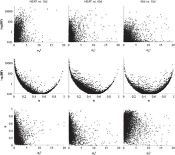
Taking the estimates from the analysis performed on uterus samples as an example (Figure 1), our results can be straightforwardly characterized by plotting the dispersion pattern of the BF itself and the two main variables involved in its parameterization, π_i and $$$\sigma _{{e\left( i \right)}}^{2} $$$. As expected, $$$\sigma _{{e\left( i \right)}}^{2} $$$ estimates accumulated to the left boundary of the positive parametric space (lower and upper rows, Figure 1), resulting in a shaped exponential pattern with minimum incidence of large variances (e.g. 1.4% (HEAT v. 15d) to 3.2% (45d v. 15d) of $$$\sigma _{{e\left( i \right)}}^{2} $$$ estimates were >5) and without showing a clear linkage with realized $$${\rm{B}}{{{\rm{F}}}_{{\rm{HE}}/{\rm{H}}{{{\rm{O}}}_i}}}$$$ (Figure 1, upper row). Conversely, π_i estimates distributed across all the parametric space (i.e. from 0 to 1) and showed a clear linkage with $$${\rm{B}}{{{\rm{F}}}_{{\rm{HE}}/{\rm{H}}{{{\rm{O}}}_i}}}$$$. As previously reported by Casellas and Varona (Reference Casellas and Varona2008), $$${\rm{B}}{{{\rm{F}}}_{{\rm{HE}}/{\rm{H}}{{{\rm{O}}}_i}}}$$$ resulted in a very characteristic U-shaped pattern when plotted against π_i (Figure 1, medium row), increasing $$${\rm{B}}{{{\rm{F}}}_{{\rm{HE}}/{\rm{H}}{{{\rm{O}}}_i}}}$$$ with extreme values of π_i (i.e. π_i tending to 0 or 1) and decreasing with intermediate estimates of π_i. Both $$$\sigma _{{e\left( i \right)}}^{2} $$$ and π_i gave us a detailed idea about the overall dispersion pattern of gene expression within each tissue and reproductive stage (Figure 1, lower row). Focusing on uterus, HEAT v. 15d and HEAT v. 45d analyses provided a skewed distribution of both $$$\sigma _{{e\left( i \right)}}^{2} $$$ and π_i, with a higher incidence of small π_i estimates and suggesting an increase of the average $$$\sigma _{{e\left( i \right)}}^{2} $$$ with smaller π_i. Both results indicated a smaller residual variability in gene expression during heat when compared with further gestational progress (i.e. 15d and 45d), which suggested a higher need for accurate genetic regulation during this initial reproductive stage. The last comparison (45d v. 15d) tended to show a higher incidence of large π_i values (i.e. closer to 1), which was indicative of a smaller overall residual dispersion of gene expression at 15d than at 45d. As a whole, these plots showed a regular temporal trend across heat and gestation in sows, suggesting that the variability of the overall gene expression increased with time, at least from heat to 45d of gestation. Very similar plots and the same overall trends were observed in both ovary and hypophysis tissues (results not shown).

Figure 1

Plots of the pairwise distribution of log($$${\rm{B}}{{{\rm{F}}}_{{\rm{HE}}/{\rm{H}}{{{\rm{O}}}_i}}}$$$), $$$\sigma _{e}^{2} $$$ and π parameters in the uterus.

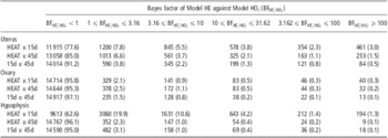
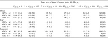
As shown in Table 2, most of the analyzed probes did not reveal relevant departures from the null hypothesis of homogeneous residual variance ($$${\rm{B}}{{{\rm{F}}}_{{\rm{HE}}/{\rm{H}}{{{\rm{O}}}_i}}}\, \less \,1$$$), ranging between 77.6% and 91.2% of the total in uterus, 95.8% and 97.1% in ovary and 62.6% and 96.1% in hypophysis. Nevertheless, the main result was not these non-heterogeneous probes but the 2.9% to 37.4% of probes providing statistical evidence of dispersion-related differential gene expression. Note that within-probe heterogeneous residual variances were previously reported when comparing great ape tissue samples (Casellas and Varona, Reference Casellas and Varona2008), although our results contribute the first evidence of within-probe heteroskedasticity in a domestic species of mammals. Following Jeffreys’ (Reference Jeffreys1984) scale of evidence for BFs, 1.5% to 19.9% of probes provided almost irrelevant evidence favoring Model HE ($$${\rm{1}}\,\leqslant \,{\rm{B}}{{{\rm{F}}}_{{\rm{HE}}/{\rm{H}}{{{\rm{O}}}_i}}}\,\leqslant \,3.16$$$), whereas substantial (0.8% to 10.6%; $$${\rm{3}}{\rm{.16}}\,\leqslant \,{\rm{B}}{{{\rm{F}}}_{{\rm{HE}}/{\rm{H}}{{{\rm{O}}}_i}}}\,\leqslant \,10$$$), strong (0.2% to 4.2%; $$${\rm{10}}\,\leqslant \,{\rm{B}}{{{\rm{F}}}_{{\rm{HE}}/{\rm{H}}{{{\rm{O}}}_i}}}\,\leqslant \,31.62$$$), very strong (0.1% to 2.3%; $$${\rm{31}}{\rm{.62}}\,\leqslant \,{\rm{B}}{{{\rm{F}}}_{{\rm{HE}}/{\rm{H}}{{{\rm{O}}}_i}}}\, \less \,100$$$) and decisive (0.1% to 3.0%; $$${\rm{B}}{{{\rm{F}}}_{{\rm{HE}}/{\rm{H}}{{{\rm{O}}}_i}}}\,\geqslant \,{\rm{100}}$$$) results must be highlighted in our study. These estimates reported a remarkable incidence of dispersion-related differential gene expression in sows, which were revealed in all three biological tissues included in our study (i.e. ovary, uterus and hypophysis) and across all the reproductive stages (i.e. HEAT, 15d and 45d of pregnancy; Table 1).

Table 2

Distribution of the number of probes (and percentage) for each analysis according to Jeffreys’ (Reference Jeffreys1984) scale of evidence for Bayes factors

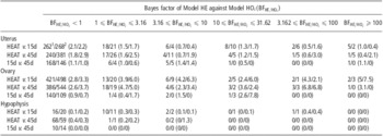
One could hypothesize that this between-groups heterogeneity of the residual variance of gene expression could be linked to scale effects because of differential gene expressions in terms of mathematical expectations. Nevertheless, this hypothesis was discarded by the results shown in Table 3. Only 0% to 7.5% of the genes with larger than one $$${\rm{B}}{{{\rm{F}}}_{{\rm{HE}}/{\rm{H}}{{{\rm{O}}}_i}}}$$$ for heterogeneous residual variances also revealed relevant differential gene expressions in terms of mathematical expectations at a posterior probability of 95% (see Casellas et al. (Reference Casellas, Ibáñez-Escriche, Martínez-Giner and Varona2008) for additional details on the calculation of this posterior probability). These results agreed with Casellas and Varona (Reference Casellas and Varona2008) and, although they cannot be extrapolated to all microarray experiments, they suggest that heterogeneous residual patterns could be a biological phenomenon of special interest in further analyses of gene expression data in the swine species, independent from scale-effect disturbances.

Table 3

Distribution of the number (and percentage) of probes with mean-related differential expression on the dispersion-related categories defined by the Bayes factor of Model HE against Model HO_i ($$${\rm{B}}{{{\rm{F}}}_{{\rm{HE}}/{\rm{H}}{{{\rm{O}}}_i}}}$$$)

¹Comparison between lowly prolific sows.

²Comparison between highly prolific sows.

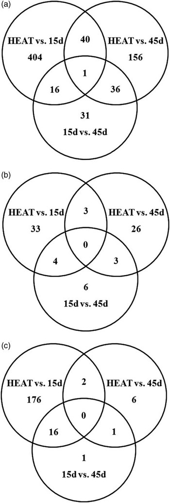
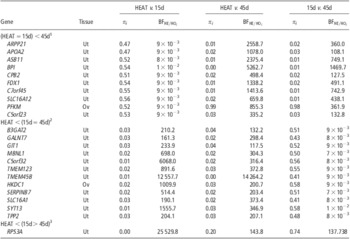
Venn diagrams provided evidence of a higher incidence of heterogenically expressed genes (with $$${\rm{B}}{{{\rm{F}}}_{{\rm{HE}}/{\rm{H}}{{{\rm{O}}}_i}}}\,\geqslant \,{\rm{100}}$$$) in uterus than in ovary or hypophysis (Figure 2), although only one gene in uterus (RPS3A; Table 4) revealed decisive evidence of heteroskedasticity in all three pairwise comparisons between reproductive stages. This gene, which encodes for the 40S ribosomal protein S3a of the small ribosomal subunit and has been linked to apoptosis and cell differentiation phenomena (Naora and Naora, Reference Naora and Naora1999), showed greater gene expression variability at 15d than at 45d and also at 45d compared with HEAT. Regarding the remaining genes with decisive evidence of heteroskedasticity or homoskedasticity in all three pairwise comparisons (Table 4), they were linked to multiple biological processes and metabolic pathways, suggesting that dispersion-specific differential gene expression could be widely distributed across the whole genome. Although the main target of this research was not focused on the identification of specific heteroskedastic genes but on checking for the suitability of this phenomenon, and its incidence in the whole genome of swine, probes shown in Table 4 represent a very promising starting point for identifying the genetic mechanisms involved in the regulation of gene transcription on a dispersion basis. Moreover, commonly used housekeeping genes such as GAPDH, HMBS, RPL32, SDHA and YWHAZ (Vandesompele et al., Reference Vandesompele, De Preter, Pattyn, Poppe, Van Roy, De Paepe and Speleman2002) were also included in the analysis and none of them showed statistically relevant dispersion-specific differential gene expression; this provided additional confidence about differentially expressed genes shown in Table 4.

Figure 2

Venn diagrams accounting for the number of highly heteroskedastic probes ($$${\rm{B}}{{{\rm{F}}}_{{\rm{HE}}/{\rm{H}}{{{\rm{O}}}_i}}}\, \great \,{\rm{100}}$$$) in uterus (a), ovary (b) and hypophysis (c).

Table 4

Summary of probes with decisive evidence of heterogeneous ($$${\rm{B}}{{{\rm{F}}}_{{\rm{HE}}/{\rm{H}}{{{\rm{O}}}_i}}}\, \great \,{\rm{100}}$$$) and/or homogeneous ($$${\rm{B}}{{{\rm{F}}}_{{\rm{HE}}/{\rm{H}}{{{\rm{O}}}_i}}}\, \less \,{\rm{0}}{\rm{.01}}$$$) residual variances in all three pairwise comparisons

Ut = uterus; Ov = ovary.

Note that 118 (uterus) and 161 (ovary) probes with homogeneous residual variances ($$${\rm{B}}{{{\rm{F}}}_{{\rm{HE}}/{\rm{H}}{{{\rm{O}}}_i}}}\, \less \,{\rm{0}}{\rm{.01}}$$$) across all tissues have been omitted.

¹Residual variances were homogeneous between HEAT and 15d, but were heterogeneous between these two groups and 45d.

²Residual variances were homogeneous between 15d and 45d, but were heterogeneous between these two groups and HEAT.

³Residual variances were heterogeneous across all groups, greater in 15d than in 45d, and greater in 45d than in HEAT.

As recently demonstrated at a gene-specific level (Lo and Gottardo, Reference Lo and Gottardo2007), an accurate modeling of residual dispersion patterns allows for a more realistic fit of gene expression data, reducing the rate of false positives when differential gene expression is characterized in terms of mathematical expectations or their differences (Kendziorski et al., Reference Kendziorski, Newton, Lan and Gould2003; Newton et al., Reference Newton, Noueiry, Sarkar and Ahlquist2004; Lo and Gottardo, Reference Lo and Gottardo2007). Moreover, the analysis of heterogeneous residual dispersion patterns opens up promising research possibilities within the gene expression framework, where heterogeneity in residual variability could be viewed as an alternative and plausible characterization of differential expression patterns. The current study provided the first evidence of massive heteroskedasticity for gene expression in the swine species, a phenomenon that must be accurately considered in further studies in order to provide a detailed characterization of the genetic architecture and regulation of domestic pigs. Moreover, and if confirmed in future analyses, the list of genes provided in Table 4 must be considered as an appealing starting point for a deeper understanding of the genetic pathways involved in sow reproduction, and may reveal dispersion-related regulatory mechanisms.