



1. Introduction
Accurate prediction of transition location is critical for aerodynamic designs of hypersonic vehicles, as the wall friction and heat flux undergo remarkable increase during the transition process. This task becomes even more challenging when the boundary layer features a blunt leading edge, a common design choice for hypersonic vehicles to prevent damage from the extreme heat loads at the stagnation point. Wind-tunnel experiments (Stetson Reference Stetson1967, Reference Stetson1983; Lysenko Reference Lysenko1990; Jewell & Kimmel Reference Jewell and Kimmel2017; Borovoy et al. Reference Borovoy, Radchenko, Aleksandrov and Mosharov2022) have revealed that the effect of nose bluntness on transition location is not monotonic. For configurations with relatively small bluntness, an increase in nose radius leads to a delay in transition; however, the opposite effect occurs when the nose radius surpasses a certain threshold. This phenomenon, known as the transition reversal phenomenon, is influenced by several factors, including the Mach number, the Reynolds number and the level of background noise.
To elucidate the physical mechanism underlying the transition reversal phenomenon, instability analyses of hypersonic boundary layers over blunt cones or wedges were conducted, revealing that increasing nose bluntness suppresses the growth rates of Mack modes, and the unstable Mack modes completely vanish once the nose radius exceeds a certain threshold (Malik et al. Reference Malik, Spall and Chang1990; Lei & Zhong Reference Lei and Zhong2012; Zhong & Wang Reference Zhong and Wang2012; Jewell & Kimmel Reference Jewell and Kimmel2017; Jewell et al. Reference Jewell, Kennedy, Laurence and Kimmel2018; Wan et al. Reference Wan, Chen, Tu, Xiang, Yuan and Duan2023). This scenario features a natural transition route, where normal instability modes dominate the accumulation of perturbations during the laminar phase. An integration of the growth rate along the streamwise direction from the neutral position confirms the delay in transition onset as the nose radius is increased from a very sharp tip configuration, effectively explaining the experimental observations for configurations with small nose radii.
Additionally, an entropy layer forming from the nose region, characterised by a high entropy or density gradient, can support an inviscid entropy-layer instability (Reshotko & Khan Reference Reshotko and Khan1980; Dietz & Hein Reference Dietz and Hein1999; Fedorov & Tumin Reference Fedorov and Tumin2004). It was found that the growth rate of the entropy-layer mode intensifies with increase of the nose radius. Although this mode emerges early around the nose region, its growth rate is typically low, making it unlikely to reach a finite-amplitude state unless the background noise is exceptionally high (Zhao & Dong Reference Zhao and Dong2025).
In addition to natural transition, bypass transition offers an alternative route that does not rely on normal instability modes. In this process, freestream perturbations, such as acoustic, vortical and entropy perturbations, enter the boundary layer and excite longitudinal streaky perturbations. Although these perturbations are composed of stable normal modes, their non-orthogonal nature allows them to exhibit transient growth due to the lift-up mechanism (Brandt et al. Reference Brandt, Schlatter and Henningson2004). These perturbations are also known as non-modal perturbations. While the growth of these non-modal perturbations is not successive, they can still accumulate to a nonlinear saturation state if (i) the level of freestream forcing, or (ii) the transient amplification rate, is sufficiently high. Notably, these non-modal perturbations are generally of low-frequency nature, which alone is insufficient to trigger transition directly through nonlinear cascade mechanisms. However, they can support secondary instabilities that exhibit high frequencies and high growth rates, allowing them to rapidly reach a nonlinear phase and eventually trigger the bypass transition.
Several theoretical frameworks have been established to predict bypass transition. The optimal growth theory emerged as a pioneering study to describe the transient growth of non-modal perturbations (Andersson et al. Reference Andersson, Berggren and Henningson1999; Paredes et al. Reference Paredes, Choudhari and Li2018; Quintanilha et al. Reference Quintanilha, Paredes, Hanifi and Theofilis2022). In this theory, the evolution of non-modal perturbations is formulated as an optimisation problem, employing an adjoint method to maximise energy amplification over a specified time period or spatial range. Subsequently, this optimisation process can be approached as an input–output computation using resolvent analysis (Towne et al. Reference Towne, Rigas, Kamal, Pickering and Colonius2022). While the optimal growth theory effectively identifies the streaky structure from the output perturbation profile, it does not take into account the receptivity process. This often results in an unphysical input perturbation profile and an overestimation of the maximum amplification rate (Zhao & Dong Reference Zhao and Dong2025).
The boundary-region equation appears as a more rational framework for considering the receptivity and evolution of non-modal perturbations. This approach employs an asymptotic matching technique to describe perturbations from the sharp leading edge to the downstream boundary layers. The linear and nonlinear evolution of non-modal perturbations in incompressible boundary layers over thin flat plates were studied by Leib et al. (Reference Leib, Wundrow and Goldstein1999) and Ricco et al. (Reference Ricco, Luo and Wu2011), respectively. More recently, this framework was extended to include the receptivity and nonlinear evolution of Görtler instabilities in compressible concave boundary layers (Xu et al. Reference Xu, Ricco and Marensi2024). While the boundary-region equation provides an effective means for formulating the early stages of bypass transition, it faces limitations when applied to boundary layers with blunt noses. In particular, the presence of the detached bow shock and the entropy layer in hypersonic boundary layers poses challenges in matching perturbations from the stagnation point to the downstream boundary layers.
To address this limitation, Zhao & Dong (Reference Zhao and Dong2025) developed an innovative shock-fitting harmonic linearised Navier–Stokes (SF-HLNS) approach. This method offers two key advantages: (i) it employs a Fourier transform with respect to time and the spanwise coordinate, reducing the four-dimensional system (three dimensions in space, and one dimension in time) to a two-dimensional one; and (ii) it employs the shock-fitting technique to accurately describe the interaction between freestream perturbations and the bow shock. With this high-efficiency and high-accuracy approach, they systematically studied the receptivity of non-modal perturbations. Their findings revealed that an increase in nose bluntness leads to an enhanced amplification rate of non-modal perturbations, qualitatively aligning with experimental observations for cases with relatively large bluntness. However, the SF-HLNS method alone cannot quantitatively predict the location of bypass transition, as it does not account for nonlinearity.
Downstream of the rapidly distorting leading-edge region, perturbations in a smooth-surface boundary layer exhibit slowly varying shape functions and wavelengths. Under these conditions, the viscous terms involving second-order streamwise derivatives become negligible, justifying the use of the parabolised stability equations (PSE) (Herbert Reference Herbert1997). By retaining triadic interaction terms among Fourier modes, one arrives at the nonlinear PSE (NPSE) formulation (Zhao et al. Reference Zhao, Zhang, Liu and Luo2016; Song et al. Reference Song, Zhao and Dong2023a , Reference Song, Dong, Zhao, Chu and Wu2024). Consequently, in the study of bypass transition, when the linear non-modal perturbations are excited in the boundary layer, the NPSE provide an efficient and accurate tool for capturing their subsequent nonlinear evolution downstream.
Once the non-modal streaks saturate at finite amplitude, small-scale perturbations emerge and undergo rapid growth via secondary instability (SI) mechanisms (Herbert Reference Herbert1988; Andersson et al. Reference Andersson, Brandt, Bottaro and Henningson2001; Ricco et al. Reference Ricco, Luo and Wu2011). These disturbances amplify into localised turbulent spots that convect downstream, merge, and ultimately lead to breakdown of the streaks, eventually causing the transition to turbulence (Zhang et al. Reference Zhang, Dong and Zhang2018; Wu Reference Wu2023). This SI can be predicted through bi-global stability analysis (BSA) of the streaky base flow (Han et al. Reference Han, Yuan, Dong and Fan2021; Song et al. Reference Song, Dong and Zhao2023b , Reference Song, Dong, Zhao, Chu and Wu2024).
Recently, Guo et al. (Reference Guo, Hao and Wen2025) carried out direct numerical simulations (DNS) on the hypersonic boundary-layer transition forced by freestream slow acoustic waves. Although the transition reversal phenomenon was reproduced, there is still a need for theoretical transition prediction approaches that offer higher efficiency and clearer understanding of the underlying physical mechanisms. Unlike natural transition, where the laminar phase is dominated by the amplification of linear normal modes and can be predicted by the conventional e-N method, bypass transition still lacks a complete predictive framework. Two key challenges are: (i) the amplitude accumulation of low-frequency non-modal perturbations, which is highly sensitive to freestream forcing; and (ii) the requirement to know the nonlinear streaky base flow before estimating SI growth. Addressing these processes thus demands a multi-method approach. In this paper, we present a comprehensive framework for predicting bypass transition over blunt bodies with relatively high nose radii, based on the experimental configuration of Borovoy et al. (Reference Borovoy, Radchenko, Aleksandrov and Mosharov2022). We will validate our predictions through direct comparison with their measured transition locations.
The rest of this paper is organised as follows. In
 $\S\,$
2, we describe the physical model and numerical methods used to predict bypass transition. Section 3 introduces the numerical results, including the base flow in
 $\S\,$
3.1, the entropy-layer instability in
 $\S\,$
3.2, the estimate of the background noise level in
 $\S\,$
3.3, the excitation of non-modal perturbations for varying controlling parameters in
 $\S\,$
3.4, the nonlinear evolution of streaks in
 $\S\,$
3.5, the SI analysis in
 $\S\,$
3.6, and the comparison with the experimental data in
 $\S\,$
3.7. Finally, conclusions and discussions are offered in
 $\S\,$
4.
2. Description of the prediction framework for bypass transition and the physical model
2.1. Outlines of the bypass transition prediction method
As illustrated above, the bypass transition in blunt-nose boundary layers occurs through three critical steps: (i) the receptivity of non-modal perturbations resulting from external forcing by the oncoming stream; (ii) the transient growth and nonlinear evolution of streaky non-modal perturbations within the boundary layer; and (iii) the accumulation of secondary instabilities that triggers the breakdown of the streaky flow. To establish a rational transition prediction method, we will quantify these three key processes using the following approaches.
-
(i) The SF-HLNS approach will be employed to describe the entrainment of freestream low-frequency perturbations into the boundary layers through their interaction with the bow shock, followed by quantifying the receptivity of the boundary-layer perturbations. While the freestream forcing is broadband, a single representative frequency–spanwise-wavenumber pair, chosen to correspond to the most amplified downstream streaks, is employed to demonstrate the essential response of boundary layer to freestream forcing. A detailed description is provided in
 $\S\,$
2.3.2.
-
(ii) The NPSE approach will be used to calculate the nonlinear evolution of boundary-layer perturbations initiated by small-amplitude disturbances excited during the receptivity process; further details are available in
$\S\,$
2.3.3. -
(iii) The non-modal streaks computed with NPSE alone do not directly trigger bypass transition. However, they can support secondary instabilities that exhibit high growth rates. The NPSE framework is not suitable for capturing the excitation of these SI modes, as their development involves rapid streamwise variation of perturbation profiles, a regime that falls outside the slow-variation assumption underlying the NPSE. Therefore, the BSA approach will be employed to determine the growth rates of secondary instabilities once the primary perturbations reach a finite-amplitude state, enabling us to predict the onset of transition based on the accumulated amplification factor of these instabilities. Additional details can be found in
$\S\,$
2.3.4.


 $(a)$
Sketch of the physical model.
 $(b)$
Side view of computational domains for (I) SF-HLNS, (II) NPSE and (III) BSA.

Figure 1. Long description
Panel A: A three-dimensional diagram showing the physical model of a blunt plate with various labeled components. The diagram includes freestream slow acoustic perturbations entering from the left, interacting with the blunt plate. Key components include the base-flow velocity profile, base-flow entropy profile, detached bow shock wave, entropy layer, boundary layer, linear/nonlinear streak, secondary-instability mode, and transition onset. The diagram illustrates the flow dynamics and transition processes around the blunt plate. Panel B: A two-dimensional diagram showing the computational domains for SF-HLNS, NPSE, and BSA. The diagram includes a bow shock and is divided into three domains: (I) SF-HLNS domain, (II) NPSE domain, and (III) BSA domain. The axes are labeled with x and y, and the diagram shows the spatial extent and boundaries of each computational domain.
2.2. Physical model
For demonstration, we choose a hypersonic boundary-layer flow over a blunt plate as the physical model, as sketched in figure 1(a). This model was also adopted in the experimental study in Borovoy et al. (Reference Borovoy, Radchenko, Aleksandrov and Mosharov2022), whose experimental data will serve to validate our transition prediction method. The mean flow field is characterised by three distinct layers: a shock layer detached from the body surface, an inviscid entropy layer exhibiting a significant rise in entropy, and a viscous boundary layer adjacent to the wall. Notably, in all the case studies that we considered, the entropy layer remains consistently thicker than the boundary layer throughout the entire domain of interest. Following the experimental set-up, we introduce a set of slow acoustic perturbations into the oncoming stream, which are assumed to be linearly independent across different Fourier components. Upon interacting with the detached shock wave, post-shock perturbations, including the acoustic, entropy and vortical disturbances, are generated in the potential region, which in turn can excite perturbations within the boundary layer. In this study, we consider relatively large nose radii, thereby excluding the presence of Mack-mode instabilities in our domain of interest. Consequently, we will concentrate on the excitation and evolution of non-modal perturbations, which are typically characterised by low-frequency, three-dimensional nature. Due to the transient growth of these non-modal perturbations, even relatively weak freestream forcing can lead to the accumulation of finite-amplitude streaks in the boundary layers, which support secondary instabilities and ultimately result in a bypass transition to turbulence.
2.3. Introduction of mathematical details
To describe the physical model, we select the nose radius
 $r^*$
as the reference length, and the physical quantities – including the density
 $\rho$
, velocity field
 $\boldsymbol{u} =(u, v, w)$
, temperature
 $T$
, pressure
 $p$
, dynamic viscosity
 $\mu$
and time
 $t$
– are normalised by the freestream quantities
 $\rho ^*_{\infty }$
,
 $U^*_{\infty }$
,
 $T^*_{\infty }$
,
 $\rho ^*_{\infty }U^{*2}_{\infty }$
,
 $\mu ^*_{\infty }$
and
 $r^*/U^*_{\infty }$
, respectively. In what follows, an asterisk represents a dimensional quantity. Here, the velocity vector is defined in the Cartesian coordinate direction. For convenience, we denote
 $\boldsymbol \varphi =(\rho ,\boldsymbol{u},T,p)$
throughout this paper. The flow is governed by two dimensionless parameters, the Reynolds number and the Mach number, defined as
 \begin{align} Re=\rho ^*_{\infty }U^*_{\infty }r^*/\mu ^*_{\infty }, \quad M=U^*_{\infty }/c^*_{\infty }, \end{align}
where
 $c^*_{\infty }$
indicates the acoustic speed in the oncoming stream.
To facilitate a mathematical description of this system, we naturally introduce a dimensionless Cartesian coordinate system
 $(x,y,z)$
, with its origin located at the centre of the blunt nose shown in figure 1(b). In the numerical process of SF-HLNS, the computational domain (indicated by the red region in figure 1
b) is discretised into grid points. A corresponding computational coordinate system
 $(\xi , \eta , \zeta )$
aligned with these grid lines is defined, and the dimensionless time is denoted as
 $\tau$
. Detailed explanations concerning the numerical implementation are provided by Zhao & Dong (Reference Zhao and Dong2025). To quantify the nonlinear evolution of the non-modal perturbations, we utilise the NPSE approach (Zhao et al. Reference Zhao, Zhang, Liu and Luo2016). For this purpose, we select a trapezoidal computational domain downstream of the nose region (the blue area marked in figure 1
b), with the inflow and upper-boundary perturbations obtained directly from the SF-HLNS calculations. The vertical grid lines are oriented perpendicular to the wall surface, and a body-fitted coordinate system
 $(x,y_n,z)$
, defined with
 $y_n=y-1$
, is adopted. As the non-modal streaky perturbations undergo transient growth, their amplitudes would reach the nonlinear phase, subsequently promoting the SI with high growth rates. Thus we select an analysis domain downstream, starting from the onset location of the SI (the green region shown in figure 1
b), and predict their amplitude accumulation using the BSA (Song et al. Reference Song, Dong, Zhao, Chu and Wu2024).
The governing equations are the three-dimensional compressible Navier–Stokes (N–S) equations. We assume a perfect gas model with constant specific heat ratio
 $\gamma =1.4$
and constant Prandtl number
 $Pr=0.72$
. Additionally, we employ Sutherland’s law for viscosity. The base flow
 ${\boldsymbol \varphi }_B$
is two-dimensional, and can be determined by solving the steady N–S equations using either shock-capturing or shock-fitting techniques, both of which yield comparably accurate numerical results, as confirmed by Zhao & Dong (Reference Zhao and Dong2025).
2.3.1. Slow acoustic wave in the oncoming stream
In the conventional wind-tunnel experiments of Borovoy et al. (Reference Borovoy, Radchenko, Aleksandrov and Mosharov2022), the dominant background disturbance is the slow acoustic wave radiated from the tunnel walls (Duan et al. Reference Duan2019). Accordingly, we model the freestream perturbation as a series of harmonic acoustic waves. Each wave has frequency
 $\omega$
, and the streamwise, wall-normal and spanwise wavenumbers are given by the vector
 $\boldsymbol k=(k_1, k_2, k_3)$
. Accordingly, we can express it as
 \begin{align} \frac {\varepsilon }{2}\hat {\boldsymbol \varphi }_{\infty }\exp[{\mathrm{i}}(k_1x+k_2y+k_3z-\omega t)]+\text{c.c.}, \end{align}
where
 $\varepsilon$
denotes the amplitude of the static pressure perturbation in the oncoming stream, c.c. denotes the complex conjugate, and
 $\hat {\boldsymbol \varphi }_{\infty }=(\hat \rho _{\infty },\hat u_{\infty },\hat v_{\infty },\hat w_{\infty },\hat T_{\infty },\hat p_{\infty })$
denotes the relative magnitude of each quantity. For normalisation, we choose
 $\hat p_\infty =1$
. Typically, the dispersion relation of the slow acoustic wave is
 \begin{align} \omega =k_1- |\boldsymbol{k}| / M, \end{align}
and
 \begin{align} \hat {\boldsymbol \varphi }_{\infty }=\left ( M^2, -\frac {k_1}{|\boldsymbol k|} M, -\frac {k_2}{|\boldsymbol k|} M, -\frac {k_3}{|\boldsymbol k|} M,(\gamma -1)M^2,1 \right )\!. \end{align}
Here, we introduce two wave angles to characterise the wavenumber ratios: an inclination angle
 $\varsigma =\tan ^{-1}({k_1/k_3})$
, and an oblique angle
 $\vartheta =\tan ^{-1}(k_2/k_3)$
. Since the excited non-modal perturbations are three-dimensional, the non-zero
 $k_3$
is taken as the denominator. To solve the acoustic dispersion relation (2.3) for a spatial mode, we prescribe the frequency
 $\omega$
and the wavenumbers
 $k_2$
and
 $k_3$
, and then compute
 $k_1$
. Consequently, the controlling parameters for the freestream forcing in the following analysis are
 $\omega$
,
 $k_3$
and
 $\vartheta$
.
2.3.2. The SF-HLNS approach
Given that the receptivity process is linear yet elliptic, we can formulate this process using a harmonic linearised framework. To simplify the challenges associated with calculating shock–perturbation interactions, we employ the shock-fitting technique. As a result, we employ the SF-HLNS approach, with the computational domain defined by the red lines in figure 1(b).
Forced by the acoustic perturbation (2.2), the perturbation field
 $\boldsymbol{\varphi}'$
and the shock movement
 $H'$
are expressed in the harmonic form
 \begin{align} \boldsymbol \varphi '(\xi ,\eta ,\zeta ,\tau )&=\frac {\varepsilon }{2} \hat {\boldsymbol \varphi }(\xi ,\eta )\exp[{\mathrm{i}} (k_3\zeta -\omega \tau )]+\text{c.c.}, \\[-12pt] \nonumber \end{align}
 \begin{align} H'(\xi ,\zeta ,\tau )&=\frac {\varepsilon }{2} \hat {H}(\xi )\exp[{\mathrm{i}} (k_3\zeta -\omega \tau )]+\text{c.c.} \\[10pt] \nonumber \end{align}
Substituting (2.5) into the linearised N–S equations, we derive the SF-HLNS equation system
 \begin{align} \mathcal L_1 \hat {\boldsymbol \varphi }(\xi ,\eta ) + \mathcal L_2 \hat {H}(\xi )=0, \end{align}
where
 $\mathcal L_1$
and
 $\mathcal L_2$
are linear operators outlined in Zhao & Dong (Reference Zhao and Dong2025). The boundary conditions for system (2.6) inlude a no-slip, isothermal condition at the wall, and a linearised Rankine–Hugoniot relation at the shock, which is formulated in response to the oncoming forcing defined in (2.2). Additionally, the shock condition also incorporates the compatibility relation given by (2.39) in Zhao & Dong (Reference Zhao and Dong2025). Detailed formulation and the corresponding algebraic derivations can be found in Zhao & Dong (Reference Zhao and Dong2025).
2.3.3. The NPSE approach
In the boundary layer, non-modal perturbations experience transient growth due to the lift-up mechanism, potentially reaching a finite-amplitude state at some downstream location. Consequently, the linearised N–S equations no longer provide an adequate approximation for the evolution of these perturbations. Therefore, we need to employ the NPSE approach to address the nonlinear interactions among different Fourier components and the mean-flow distortion. As illustrated in figure 1
 $(b)$
, the NPSE calculations start from a position downstream of the nose region (denoted by
 $X_{0}$
), using the SF-HLNS solutions as the initial conditions. It should be emphasised that the NPSE approach relies on a parabolised approximation of the N–S system, which assumes that the streamwise length scale is much longer than the wall-normal length scale, such that the second-order streamwise derivative is negligible. Scaling analysis indicates that in the stagnation region (
 $(x,y)\approx (-1,0)$
), both the streamwise and wall-normal length scales are
 $O(1/Re)$
, corresponding to an elliptic region. In contrast, at the nose–plate junction, the streamwise length scale is
 $O(1)$
, while the wall-normal scale is
 $O(1/Re)$
, corresponding to a boundary-layer region where the parabolised assumption holds well. Further downstream, at locations where
 $x\sim Re$
, the streamwise and wall-normal length scales are
 $O(Re)$
and
 $O(1)$
, respectively, which also satisfy the NPSE assumption. Moreover, to ensure that the SF-HLNS calculations serve as a good approximation of the NPSE initial condition, the perturbation amplitudes at
 $X_0$
must remain sufficiently small. As will be shown in figure 9 below, a distinct linear region is observed near the NPSE inlet for each case under consideration. Therefore, initialising the NPSE computation in the vicinity of the nose–plate junction is justified, and changes in
 $X_0$
within this constrained region do not affect the perturbation calculations. For the blunt-plate model, the body-fitted coordinate system
 $(x,y_n,z)$
employed in the NPSE formulation is obtained by directly translating the original coordinate system
 $(x,y,z)$
via
 $y_n=y-1$
. Therefore, the velocity vector
 $\hat{\boldsymbol{u}}$
remains consistent between the SF-HLNS and PSE frameworks.
In the NPSE approach, we use a marching scheme to compute the perturbation profile based on its upstream information, with the numerical details outlined in our previous studies (Zhao et al. Reference Zhao, Zhang, Liu and Luo2016; Song et al. Reference Song, Zhao and Dong2023a , Reference Song, Dong, Zhao, Chu and Wu2024). The perturbation profile at each streamwise position is expressed as
 \begin{align} \boldsymbol \varphi '(x,y_n,z,t)=\sum _{m=-\mathcal{M},\ n=-\mathcal{N}}^{\mathcal{M},\mathcal{N}} \hat {\boldsymbol \varphi }_{m,n}(x,y_n)\exp[ {\mathrm{i}} (nk_3 z-m\omega t)], \end{align}
where
 $m$
and
 $n$
denote the harmonic orders, and
 $\mathcal{M}$
and
 $\mathcal{N}$
denote the truncation orders. Substituting (2.7) into the N–S equations, and neglecting the
 $\partial _{x}^2$
terms, we derive the NPSE equations at each streamwise position:
 \begin{align} \mathcal{L}_3\hat {\boldsymbol \varphi }_{m,n}=f_{m,n}, \end{align}
where
 $\mathcal{L}_3$
is a parabolised operator, and
 $f_{m,n}$
denotes the nonlinear terms. For convenience, we denote each Fourier component by
 $(m,n)$
.
As will be demonstrated by the SF-HLNS calculations in § 3.4, the non-modal perturbations experience stronger amplification at lower frequencies, with stationary freestream acoustic perturbations exhibiting the highest receptivity efficiency. Therefore, in this paper, we set
 $\omega =0$
for the NPSE calculations, a configuration that is representative of low-frequency freestream forcing. In fact, for non-stationary forcing, the receptivity calculations would remain largely unchanged as long as the frequency lies within the low-frequency band. Consequently, we set
 $\mathcal{M}=0$
in (2.7) to remove the temporal harmonics. The mean-flow distortion is denoted by
 $(0,0)$
, the fundamental component is denoted by
 $(0,1) $
, and the harmonics are denoted by
 $(0,2),(0,3),\ldots $
. The truncation order of the spanwise-wavenumber harmonics is
 $\mathcal{N}=5$
.
At the inlet boundary of the NPSE computational domain,
 $x=X_0$
, where the perturbation level is small, only the
 $(0,1)$
component, obtained from the SF-HLNS calculations, is introduced. In principle, higher-order harmonics (e.g. components
 $(0,2),(0,3),\ldots $
) from SF-HLNS could also be introduced. However, doing so would substantially complicate the numerical set-up, as the amplitudes of these harmonics in the freestream would need to be adjusted to reflect a realistic wind-tunnel energy spectrum, while the essential downstream streak formation mechanism would remain unchanged. As a predictive tool, the present single-component approach is therefore both physically rational and computationally efficient. The same wall-normal mesh is used in both the SF-HLNS and NPSE computations, minimising numerical errors that could arise from discretisation differences. Although the initial harmonics are set to zero, they are quickly generated through the self-nonlinear interaction of the fundamental mode. After a short adjustment region, the weakly nonlinear phase would be reached, with the harmonics being determined solely by the local fundamental mode. Because the amplification of non-modal perturbations is confined to the boundary layer, disturbances in the potential flow region above the boundary layer remain essentially unchanged. Hence Dirichlet boundary conditions are imposed at the upper boundary (
 $y_n=Y_n$
) for the fundamental mode, with values prescribed according to the SF-HLNS results. For the mean-flow distortion and all harmonics, the values at the upper boundary are set to zero, except for
 $\hat v_{0,0}$
, which satisfies a zero-gradient condition. Again, the no-slip, isothermal boundary conditions are applied at the wall (
 $y_n=0$
).
2.3.4. The BSA approach
Since low-frequency non-modal perturbations do not break down themselves, the SI modes supported by the nonlinear streaky profile play a crucial role in triggering the bypass transition. To predict the transition onset, the accumulation of the SI amplitudes should be quantified. Thus we perform the BSA based on the mean flow distorted by the strong non-modal streaks, as sketched in the green region in figure 1
 $(b)$
. The streaky profile at a position
 $x$
is expressed as
 \begin{align} \bar {\boldsymbol \varphi }(y_n,z;x)= {\boldsymbol \varphi }_B(y_n;x) +\sum _{n=-{ \mathcal{N}}}^{ \mathcal{N}} \hat {\boldsymbol \varphi }_{0,n}(y_n;x)\, {\mathrm{e}} ^{{\mathrm{i}} n k_3 z}, \end{align}
where
 $\hat {\boldsymbol \varphi }_{0,n}$
is obtained from the NPSE calculation.
Since the length scale of the streaky base flow (2.9) is much greater than that of the SI, we can introduce the parallel-flow assumption and express the SI mode as
 \begin{align} \boldsymbol \varphi '_{SI}(x,y_n,z,t)= {\mathrm{e}}^{{\mathrm{i}} (\alpha {x}-\bar \omega t)} \, {\mathrm{e}}^{{\mathrm{i}} \sigma _d k_3 z}\,\hat {\boldsymbol \varphi }_{SI}(y_n,z) +\text{c.c.}, \end{align}
where
 $\bar \omega$
and
 $\alpha$
denote the frequency and the streamwise wavenumber, respectively, and
 $\sigma _d\in [0,0.5]$
denotes the detuning parameter. Here,
 $\sigma _d=0$
denotes the fundamental SI modes, while
 $\sigma _d=0.5$
denotes the subharmonic SI modes. For a temporal mode, we specify
 $\alpha \in \mathbb{R}$
, and calculate
 $\bar \omega =\bar \omega _r+\mathop {\mathrm{i}}\nolimits \bar \omega _i \in \mathbb{C}$
, where
 $\bar \omega _i$
represents the temporal growth rate. Conversely, for a spatial mode, we specify
 ${\bar \omega } \in \mathbb{R}$
, and calculate
 $\alpha =\alpha _r+\mathop {\mathrm{i}}\nolimits \alpha _i \in \mathbb{C}$
, where
 $-\alpha _i$
represents the spatial growth rate. It needs to be emphasised that the SI frequency
 $\bar \omega$
is much higher than that of the non-modal perturbation
 $\omega$
.
Since the N–S equations involve only first-order time derivatives but second-order spatial derivatives, temporal mode calculations are more convenient. From the linearised N–S equations, we derive a generalised eigenvalue system
 \begin{align} \mathcal{A}\, \hat {\boldsymbol \varphi }_{SI}(y_n,z)=\bar \omega \mathcal{B}\, \hat {\boldsymbol \varphi }_{SI}(y_n,z), \end{align}
where
 $\bar \omega$
appears as the eigenvalue, and the coefficient matrices
 $\mathcal{A}$
and
 $\mathcal{B}$
are readily derived from the linear equations shown in Song et al. (Reference Song, Dong, Zhao, Chu and Wu2024). The Arnoldi iterative method is employed to search the eigenvalues initially, and the Rayleigh quotient iteration method is used to confirm its accuracy, as has been used in Han et al. (Reference Han, Yuan, Dong and Fan2021) and Song et al. (Reference Song, Dong, Zhao, Chu and Wu2024).
Noting that the spatial SI mode is more relevant for the transition prediction method, we convert the temporal SI solutions to a spatial mode using the following looping method.
-
(i) Provide an initial guess for
$\alpha$
. -
(ii) Solve for
$\bar \omega (\alpha )$
from (2.11). -
(iii) Calculate
${\rm d}\bar \omega /{\rm d}\alpha$
by introducing a small perturbation to
$\alpha$
, namely,
${\rm d}\bar \omega /{\rm d}\alpha = [\bar \omega (\alpha +\epsilon _\alpha )-\bar \omega (\alpha )]/\epsilon _\alpha$
. -
(iv) Update
$\alpha$
using the Newton iterative scheme, and repeat step (ii). The iteration is terminated when the computed
$\bar \omega$
is real and matches the specified value.


Once the spatial growth rate of SI
 $-\alpha _i(x)$
at each position
 $x$
is obtained, its amplitude amplification can be determined through spatial integration. For an SI mode with a frequency
 $\bar \omega$
, we define an amplification factor
 \begin{align} N({x};\bar \omega )=\int _{x_n}^{{x}}- \alpha _i(\bar {x};\bar \omega )\, \mathrm{d}\bar x, \end{align}
where
 $x_n$
represents the neutral position of SI for frequency
 $\bar \omega$
. The implication is that this SI is amplified
 $\mbox{e}^N$
times from the neutral position to
 $x$
. According to the classical e-N method, the transition onset may be prescribed by the position where
 \begin{align} \max _{\bar \omega }\{N({x},\bar \omega )\}=N_{\textit{tr}},\end{align}
with
 $N_{\textit{tr}}$
being an empirical constant representing the transition threshold. Note that the receptivity of secondary instabilities in the streaky base flow is not considered in this study, because the high growth rates of these instabilities imply that their amplitude accumulation is dominated by the integration of the growth rate; the error introduced by assuming identical initial amplitudes at the neutral point is therefore small.
3. Numerical results
3.1. Base flow
Experimental data from Borovoy et al. (Reference Borovoy, Radchenko, Aleksandrov and Mosharov2022) exhibit two opposing trends in boundary-layer transition: in one, increasing nose radii delays transition; in the other, it leads to earlier transition. In the present study, we focus on the latter behaviour, examining five configurations listed in table 1. All cases employ an oncoming Mach number
 $M=5$
, unit Reynolds number
 $Re_{\infty }^*:=\rho _\infty ^*U_{\infty }^*/\mu ^*_\infty =5.80\times 10^7$
m−1, total temperature
 $T_{0}^*=464$
K, and static temperature
 $T_\infty ^*=77.33$
K, with wall temperature
 $T_w^*=293$
K (corresponding to
 $T_w=T_w^*/T_{\infty }^*=3.79$
). The measured transition locations
 $x_{\textit{tr}}$
(second-to-last column) and corresponding transitional Reynolds numbers
 ${Re_{\textit{tr}}}:=\rho _\infty ^*U_\infty ^*{x_{\textit{tr}}} r^*/\mu _\infty ^*$
(last column) confirm that increasing the nose radius shifts the transition position upstream, thereby reducing the streamwise extent
 $x_L$
needed for the base-flow calculation.
Parameters for case studies and experimental transition locations.

Table 1. Long description
A table comparing nose radius, Reynolds number, and transition characteristics for different cases. The table has five rows and six columns. The columns are labeled Nose radius, Reynolds number, Computational domain outlet, Transition onset, and Transitional Reynolds number. The row labels are Case A, Case B, Case C, Case D, and Case E. Row 1: Case A, Nose radius 1.20 millimeters, Reynolds number 0.696 times 10 to the power of 5, Computational domain outlet 250, Transition onset 129, Transitional Reynolds number 8.98 times 10 to the power of 6. Row 2: Case B, Nose radius 1.80 millimeters, Reynolds number 1.044 times 10 to the power of 5, Computational domain outlet 150, Transition onset 72, Transitional Reynolds number 7.52 times 10 to the power of 6. Row 3: Case C, Nose radius 2.00 millimeters, Reynolds number 1.160 times 10 to the power of 5, Computational domain outlet 150, Transition onset 43, Transitional Reynolds number 4.99 times 10 to the power of 6. Row 4: Case D, Nose radius 2.60 millimeters, Reynolds number 1.508 times 10 to the power of 5, Computational domain outlet 80, Transition onset 30, Transitional Reynolds number 4.52 times 10 to the power of 6. Row 5: Case E, Nose radius 3.00 millimeters, Reynolds number 1.740 times 10 to the power of 5, Computational domain outlet 80, Transition onset 23, Transitional Reynolds number 4.00 times 10 to the power of 6.
(
 $a$
) Contours of the local Mach number
 $\bar M$
and the entropy increment
 $\Delta s$
in the
 $x{-}y$
plane for case A (not to scale). (
 $b$
,
 $c$
) Wall-normal profiles of
 $u_B$
and
 $T_B$
in regular and logarithmic scales, respectively, where
 $\delta _{\textit{EL}}$
and
 $\delta _{\textit{BL}}$
mark the edges of the entropy and boundary layers, respectively.

Figure 2. Long description
Panel A: A contour plot shows the local Mach number and entropy increment in the plane for case A. The color scale for the local Mach number ranges from 0 to 2.55, and the color scale for the entropy increment ranges from 0.2 to 3.2. The plot highlights regions of shock and changes in entropy. Panel B: A line graph displays wall-normal profiles of T subscript B in regular scale. The x-axis represents u subscript B, ranging from 0 to 1.0, and the y-axis represents y subscript n, ranging from 0 to 15. Different lines represent different x values (50, 100, 200), with delta subscript EL and delta subscript BL marked by horizontal dashed lines. Panel C: Another line graph shows wall-normal profiles of T subscript B in logarithmic scale. The x-axis represents u subscript B, ranging from 0 to 1.0, and the y-axis represents the natural logarithm of y subscript n, ranging from -6 to 6. Different lines represent different x values (50, 100, 200), with delta subscript EL and delta subscript BL marked by horizontal dashed lines.
To compute the blunt-plate base flow, we employ an in-house shock-fitting DNS code, previously used in Zhao & Dong (Reference Zhao and Dong2025). The upper boundary of the computational domain is located at the bow shock, as sketched in figure 1. Each simulation utilises a grid of
 $551\times 301$
points. A resolution study for case A is presented in figure 20(a) in Appendix A. Furthermore, as shown in figure 21 in Appendix A, the accuracy of the shock-fitting approach is corroborated by comparing with the shock-capturing DNS results. These comparisons confirm that the upper boundary of the shock-fitting computational domain corresponds precisely to the bow shock location. Figure 2(a) presents contours of the local Mach number
 $\bar M=M\sqrt {|\boldsymbol{u}_B|^2/{{T}_B}}$
and the normalised entropy increment
 $\Delta s=[\gamma /(\gamma -1)]\ln T_B-\ln(\gamma M^2 p_B)$
for case A. In the nose region, the Mach number decreases significantly as the flow passes through the strong, nearly normal shock wave, corresponding to a notable entropy increase in this area. As the distance from the leading edge increases, however, the shock angle gradually decreases, causing a milder drop in Mach number in the downstream post-shock region. Meanwhile, the low-
 $\bar M$
region formed around the nose extends downstream, generating a distinct entropy layer characterised by a pronounced entropy rise beneath the high-
 $\bar M$
region. The outer edge of this entropy layer, marked as
 $\delta _{\textit{EL}}$
, is illustrated by the dot-dashed line in figure 2(a). In fact, both the entropy layer itself and the region between its outer edge and the shock are inviscid. A viscous boundary layer emerges only in the immediate vicinity of the wall, with its outer boundary denoted by
 $\delta _{\textit{BL}}$
. Here, the means to determine the thicknesses of the entropy and boundary layers follow those in Zhao & Dong (Reference Zhao and Dong2025).
Although the boundary layer is not clearly visible in the
 $\bar M$
-contour plot, its presence is evident from the high gradients of
 $u_B$
and
 $T_B$
seen in their vertical profiles shown in figures 2(b) and 2(c). Notably, the boundary-layer thickness expands as the flow moves downstream. By comparing these results with those from other cases (not shown), it is observed that an increase in Reynolds number produces a thinner boundary layer. In contrast, the entropy layer remains largely unchanged due to its inviscid nature.
3.2. Modal instability analysis
For a given base-flow profile
 $u_B(y_n;x)$
and
 $T_B(y_n;x)$
, stability analysis can be carried out by solving the compressible Orr–Sommerfeld equations, as detailed in Dong et al. (Reference Dong, Liu and Wu2020). Here, we denote the frequency, streamwise wavenumber and spanwise wavenumber by
 $\omega$
,
 $\alpha$
and
 $\beta$
, respectively, and the eigenfunctions by
 $\hat {\boldsymbol \varphi }(y_n)$
. For all cases considered in this study, no unstable Mack modes are detected within the computational domain. However, unstable entropy-layer modes are identified, as shown in figure 3. The entropy-layer mode is more unstable for two-dimensional configurations. While the entropy-layer mode exhibits exponential growth at relatively high frequencies, the accumulated
 $N$
factor remains small (at most approximately 0.2) up to the outlet of the computational domain. Although the growth rate increases with increasing
 $Re$
, the accumulated
 $N$
factor becomes smaller due to the reduced length of the computational domain at higher Reynolds numbers. Such small amplification factors are insufficient to trigger transition. Therefore, we conclude that the experimentally observed transition is driven by non-modal perturbations via a bypass route.
Properties of entropy-layer modes.
 $(a{,}b)$
Contours of
 $-\alpha _i$
in the
 $\beta$
–
 $\omega$
plane at
 ${x}=25$
.
 $(c{,}d)$
Contours of the
 $N$
factor of the two-dimensional entropy-layer modes in the
 $x$
–
 $\omega$
plane. Plots are for (a,c) case A, and (b,d) case E.

3.3. Estimate of background noise
To enable a fair comparison with the experimental transition measurements, it is necessary to first estimate the spectra of freestream perturbations upstream of the bow shock. However, the noise level and power spectra of the UT-1M wind tunnel employed in Borovoy et al. (Reference Borovoy, Radchenko, Aleksandrov and Mosharov2022) were not reported in the literature. Therefore, the perturbation spectra in this study are estimated by referring to the data from other conventional wind tunnels (Wagner et al. Reference Wagner, Schülein, Petervari, Hannemann, Ali, Cerminara and Sandham2018; Duan et al. Reference Duan2019; Liu et al. Reference Liu, Schuabb, Duan, Paredes and Choudhari2022).
Validation of (3.1) by wind-tunnel-noise measurements of PSD (Duan et al. Reference Duan2019), where two levels of
 $Q$
are selected. HLB: Hypersonic Ludwieg Tube Braunschweig; M6 Purdue: Purdue Boeing/U.S. Air Force Office of Scientific Research Mach-6 Quiet Tunnel;M6 NASA 20-in: NASA 20-Inch Mach 6;M8 Sandia: Sandia Hypersonic Wind Tunnel at Mach 8; M14 AEDC: Arnold Engineering Development Complex Tunnel 9.

Figure 4. Long description
A line graph displays the power spectral density (PSD) of perturbations in the boundary layer against the frequency (f star) in Hertz. The vertical axis represents PSD in units of ((p 0 s star prime divided by p 0 s star) squared per Hertz), ranging from 10 to the power of negative 14 to 10 to the power of negative 7. The horizontal axis represents frequency (f star) in Hertz, ranging from 100 to 10 to the power of 6. The graph includes multiple data lines representing different experimental conditions with varying Reynolds numbers (Re). The green solid line represents Q equals 3.5 percent, and the blue solid line represents Q equals 1.75 percent, both following Equation 3.1. Other lines represent different experimental setups such as M 6 H L B, M 6 Purdue, M 6 N A S A 20 inch, M 8 Sandia, and M 14 A E D C, each with specific Reynolds numbers. The lines show different trends, with some exhibiting higher PSD values at lower frequencies and others showing a decrease in PSD as frequency increases. The graph also includes dashed lines indicating specific frequency values (f star equals 1 and f star equals 3.5).
In wind-tunnel experiments, Pitot tubes are commonly used to measure the power spectral density (PSD) of the total pressure perturbation signal
 $p^{\ast \prime }_{0s}$
at the stagnation point. The PSD quantifies the frequency-dependent distribution of the total pressure perturbation power. We denote the normalised PSD of
 $(p^{\ast \prime }_{0s}/p^*_{0s})^2$
by
 $S^*(f^*)$
, where
 $f^{*}=\omega U^*_{\infty }/(2\pi r^*)$
represents the dimensional frequency.
As shown in figure 2 of Duan et al. (Reference Duan2019) (reproduced by the thin lines in figure 4), the PSD measurements from multiple wind-tunnel runs show good overall agreement. The spectra are characterised by three distinct scaling regions: a quasi-constant plateau at low frequencies, an intermediate region following an
 $f^{*-1}$
decay, and a high-frequency region with a steeper
 $f^{*-3.5}$
decay. The transitions between these regions occur at approximately 10 kHz and 80 kHz. To model the unified spectral shape, we propose an empirical formula based on this observed behaviour:
 \begin{align} {S^*}(f^*)= {A_S\, S^*_0}(f^*),\quad {S^*_0}(f^*)=\begin{cases} {a_0}, &f^* \leqslant {10}\ \mathrm{kHz}, \\[5pt]a_1 f^{*-1}, &{10} \lt f^* \leqslant {80}\ \mathrm{kHz}, \\[5pt]{a_2} f^{*-3.5},&f^* \gt {80}\ \mathrm{kHz}, \end{cases} \end{align}
where
 $A_S$
characterises the magnitude of the normalised pressure perturbation power, and
 $S^*_0$
represents the unit distribution function, satisfying
 $\int _0^\infty {S^*_0}\,\mathrm{d}f^*=1$
, with the parameters set as
 ${(a_0,a_1,a_2)}=(0.0287\ \mathrm{kHz^{-1}},0.287,1.65\times 10^{4}\ \mathrm{kHz^{2.5}})$
. It should be noted that although medium- and high-frequency perturbations are not directly used in the receptivity calculations, their energy spectrum is needed to determine
 $(a_0,a_1,a_2)$
, which in turn affects the proportion of low-frequency energy relative to the total energy.
In conventional wind tunnels, the root mean square (RMS) of the perturbation total pressure relative to the mean total pressure at the stagnation point,
 $p^{\ast \prime }_{0s,\textit{RMS}}/p^*_{0s}$
, as measured by the Pitot tubes, is typically of the order of
 $Q=1{-}5\,\%$
(Casper et al. Reference Casper, Beresh, Henfling, Spillers, Pruett and Schneider2016). This corresponds to a PSD magnitude
 $A_S=(\sqrt {2}\,Q)^2$
, where the factor
 $\sqrt {2}$
appears to convert the RMS value to the perturbation amplitude. The thick blue curve in figure 4 represents the evaluation of (3.1) using
 $Q=1.75\,\%$
, which agrees well with the experimental measurements. To further assess the sensitivity of our transition prediction framework to background noise, we also perform calculations with twice the nominal noise level (
 $Q=3.5\,\%$
); the corresponding PSD is indicated by the thick green line in figure 4.
As reported in Borovoy et al. (Reference Borovoy, Radchenko, Aleksandrov and Mosharov2022), the total and static temperatures are
 $T_{0}^*=464$
K and
 $T_{\infty }^*=77.3$
K, respectively. For Mach number
 $M=5$
and unit Reynolds number
 ${Re^*_{\infty }}=5.80\times 10^7$
m−1, the corresponding sound speed, the freestream velocity and the density of the oncoming stream are calculated as
 $a_\infty ^*={176\ \mathrm{m\,s}^{-1}}$
,
 $U_\infty ^*={881\ \mathrm{m\,s}^{-1}}$
and
 $\rho _\infty ^*={0.348\ \mathrm{kg\,m}^{-3}}$
, respectively. Using the equation of state, we obtain the static pressure of the oncoming stream as
 $p_\infty ^*={7.72\times 10^3\ \mathrm{Pa}}$
, which can then be converted to the mean total pressure
 \begin{align} p_{0\infty }^*=p_{\infty }^* \left [1+\frac {\gamma -1}{2}M^2\right ]^{\gamma /(\gamma -1)}=4.08\times 10^6\ \mathrm{Pa}. \end{align}
As the flow passes through the bow shock, its total pressure drops sharply and then remains nearly constant in the post-shock region all the way to the stagnation point. Therefore, we can estimate the mean total pressure at the stagnation point using the Rankine–Hugoniot relation of a normal shock:
 \begin{align} p_{0s}^*={p_{0\infty }^* \left [\dfrac {(\gamma +1)M^2}{(\gamma -1)M^2+2}\right ]^{{\gamma }/({\gamma -1})} \left [\dfrac {\gamma +1}{2\gamma M^2-(\gamma -1)}\right ]^{{1}/({\gamma -1})}=2.52\times 10^5\ \mathrm{Pa}}. \end{align}
Consequently, the RMS of the perturbation total pressure at the stagnation point, measured by the Pitot tube, is
 $p^{\ast \prime }_{0s,\textit{RMS}}\approx p^*_{0s}\times Q$
.
By integrating the PSD over the low-frequency (0–10 kHz), medium-frequency (10–80 kHz) and high-frequency (
 $\gt$
80 kHz) bands, we can estimate the total pressure perturbation power for the three bands:
 ${S_{\textit{lo}w}}=\int _0^{{10}}S^*\, \mathrm{d}f^*={0.287A_S}$
,
 ${S_{\textit{mid}}}=\int _{{10}}^{{80}}S^*\, \mathrm{d}f^*={0.598A_S}$
and
 ${S_{\textit{high}}}=\int _{{80}}^\infty {S^*\, \mathrm{d}f^*=0.115A_S}$
, respectively. Thus the contributions of these three bands to the power of the total-pressure perturbation are in the following proportions:
 \begin{align} {P_{\textit{lo}w}=\frac {S_{\textit{lo}w}}{A_S}=0.287},\quad {P_{\textit{mid}}=\frac {S_{\textit{mid}}}{A_S}=0.598},\quad {P_{\textit{high}}=\frac {S_{\textit{high}}}{A_S}=0.115}. \end{align}
In our theoretical model, the non-modal streaks are intrinsically low-frequency. Therefore, we restrict our attention to perturbations with
 $f^*\leqslant {10}$
kHz, for which the perturbation level is estimated to be (noting that the RMS is the square root of the power)
 \begin{align} {\frac {p^{\ast \prime }_{0s,RMS,f^*_{\textit{lo}w}}}{p^*_{0s}}}={\frac {p^{\ast \prime }_{0s,\textit{RMS}}}{p^*_{0s}}\times \sqrt {P_{\textit{lo}w}}}=\begin{cases} {0.00938} &\mbox{for }Q={1.75}\,\%, \\[4pt]{0.0188} & \mbox{for }Q={3.5}\,\%. \end{cases} \end{align}
Since our model also incorporates the spanwise spatial-spectrum distribution, only a portion of the low-frequency RMS pressure perturbation
 $p^{\ast \prime }_{0s,\textit{RMS},f^*\leqslant 10\ \mathrm{kHz}}$
serves as the seed for non-modal excitation. Therefore, the power spectrum is further decomposed into low-, mid- and high-wavenumber bands in each spatial direction. Given that the non-modal perturbations are characterised by short spanwise scales, the high-wavenumber components of the freestream perturbations are most relevant. Lacking direct wavenumber-spectrum measurements, we invoke Taylor’s frozen-field hypothesis, and adopt the band fractions given in (3.4). Furthermore, the wavenumbers of slow acoustic waves radiated by wind-tunnel wall turbulence in different directions are interrelated through the dispersion relation. Based on these considerations, the effective seed perturbation level can be estimated as
 \begin{align} {\frac {p^{\ast \prime }_{0s,RMS,f^*_{\textit{lo}w},k^*_{\textit{high}}}}{p^*_{0s}}}={\frac {p^{\ast \prime }_{0s,RMS,f^*_{\textit{lo}w}}}{p^*_{0s}}\times \sqrt {P_{\textit{high}}}}=\begin{cases} {0.00318} &\mbox{for }Q={1.75}\,\%, \\[4pt]{0.00638} &\mbox{for }Q={3.5}\,\%. \end{cases} \end{align}
Dependence of
 $\chi$
defined in (3.7) on (
 $a$
)
 $\omega$
(for
 $k_3=4$
) and (
 $b$
)
 $k_3$
(for
 $\omega =0$
).

The next task is to convert the total pressure perturbation
 $p^{\ast \prime }_{0s}$
at the stagnation point to the static pressure perturbation
 $p^{\ast \prime }_{\infty }$
in the oncoming stream. This can be implemented by the numerical results of SF-HLNS calculations. For simplicity, we introduce a relation characterising the ratio of the relative perturbation level of the oncoming stream to that at the stagnation point:
 \begin{align} \chi = {\frac {p^{\ast \prime }_{\infty }/p^*_{\infty }}{p^{\ast \prime }_{{0s}}/p^*_{{0s}}}}. \end{align}
Choosing cases A and E, the cases with the lowest and highest Reynolds numbers in our study, we plot the dependence of
 $\chi$
on
 $\omega$
(for
 $k_3=4$
) and
 $k_3$
(for
 $\omega =0$
) in figures 5(a) and 5(b), respectively. It is evident that
 $\chi$
varies only slightly and remains approximately 1.55. Hence the relative static-pressure perturbation in the freestream can be estimated as
 \begin{align} {\frac {p^{\ast \prime }_{\infty ,f^*_{\textit{lo}w},k^*_{\textit{high}}}}{p^*_{\infty }}}= \sqrt {2}\,\chi\, {\frac {p^{\ast \prime }_{0s,\textit{RMS},f^*_{\textit{lo}w},k^*_{\textit{high}}}}{p^*_{0s}}}= \begin{cases} {0.00697} &\mbox{for }Q={1.75}\,\%, \\ {0.0140} &\mbox{for }Q={3.5}\,\%, \end{cases} \end{align}
where the factor
 $\sqrt {2}$
converts the RMS value to the peak value of the perturbation. In our study, the pressure is normalised by
 $\rho ^*_\infty U_\infty ^{*2}$
, and then we can estimate that
 \begin{align} \varepsilon ={\frac {p^{\ast \prime }_{\infty ,f^*_{\textit{lo}w},k^*_{\textit{high}}}}{\rho ^*_\infty U_\infty ^{*2}}}=\begin{cases} {0.0002} &\mbox{for }Q={1.75}\,\%, \\ {0.0004} &\mbox{for }Q={3.5}\,\%. \end{cases} \end{align}
It should be noted that the estimate of
 $\varepsilon$
in this subsection is rather preliminary and subject to several uncertainties. First, the assumed noise levels
 $Q=1.75\,\%$
and
 $3.5\,\%$
are typical examples of many conventional wind tunnels, and may differ from that in the facility used by Borovoy et al. (Reference Borovoy, Radchenko, Aleksandrov and Mosharov2022). Second, the PSD curve-fitting procedure itself introduces additional inaccuracy. Third, the receptivity coefficient depends on both frequency and wavenumber, and representing the broadband low-frequency, high-wavenumber spectrum with a single Fourier mode may lead to quantitative discrepancies. Despite these limitations, the following analyses will present bypass transition predictions for the two representative noise levels, demonstrating that the proposed prediction framework remains robust with respect to the specific choice of freestream disturbance amplitude. We emphasise, however, that direct measurement of the facility noise spectrum is essential for the reliable interpretation of wind-tunnel transition experiments.
3.4. The SF-HLNS calculations
Using the SF-HLNS approach, we calculate the perturbation field within the region between the bow shock and the wall. As a linear approach, the resulting receptivity coefficients are independent of the background noise level as estimated in the last subsection. However, they will determine the initial conditions for the NPSE computations to be discussed in the following subsection. To validate the accuracy of the SF-HLNS solver, we additionally performed DNS by setting the freestream acoustic amplitude to be
 $10^{-8}$
for the largest bluntness configuration (case E). A comparative analysis of the SF-HLNS and DNS results is presented in this subsection.
Figures 6(a) and 6(b) present the pressure contours in the
 $x$
–
 $y$
plane for cases A and E, respectively, illustrating the dominant acoustic beam propagating through the post-shock potential region located above the entropy layer and downstream of
 $x\approx 40$
. Notably, in each plot, a weak additional wave beam is generated in the nose region and propagates into the potential flow. This is a Mach wave radiation produced as upstream disturbances propagate across the nose–plate junction, where the curvature is discontinuous. The insets highlight the perturbation pressure distribution in the nose region, characterised by pronounced gradients.
Perturbation field obtained by SF-HLNS calculations for
 $\omega =0$
and
 $\vartheta =0^{\circ }$
: (a,c,e) case A with
 $k_3=4$
, (b,d,f) case E with
 $k_3=16$
, with contours of (a,b)
 $\hat p$
, (c,d)
 $\hat u$
and (e,f)
 $\hat T$
. The DNS results for case E are marked by green dashed lines for reference.

Figures 6(c–f) present the contours of
 $|\hat u|$
and
 $|\hat T|$
, with insets magnifying the nose and boundary-layer regions. It is evident that both
 $\hat u$
and
 $\hat T$
achieve their maxima near the edge of the boundary layer, with the magnitude of
 $\hat T$
being greater. Moreover, an increase in
 $Re$
strengthens the downstream amplitude amplification of these perturbations. For validation, figures 6(b,d,f) superimpose DNS results for case E as green dashed lines. The two sets of results exhibit favourable agreement, particularly in the nose and boundary-layer regions where gradients are most pronounced.
Perturbation amplitude distributions for case A. (
 $a$
) Streamwise evolution of
 $A_u$
for
 $k_3$
varying from 1 to 10 in increments of 1, with
 $\omega =0$
and
 $\vartheta =0{^{\circ }}$
. The red curve indicates the case for
 $k_3=4$
. The vertical line indicates the experimentally observed transition onset from Borovoy et al. (Reference Borovoy, Radchenko, Aleksandrov and Mosharov2022). (
 $b$
–
 $d$
) Dependence of
 $A_u$
(solid lines) and
 $A_T$
(symbol lines) on
 $k_3$
(with
 $\omega =0$
and
 $\vartheta =0{^{\circ }}$
),
 $\omega$
(with
 $k_3=4$
and
 $\vartheta =0{^{\circ }}$
) and
 $\vartheta$
(with
 $\omega =0$
and
 $k_3=4$
) at
 ${x}$
values 50 (red), 100 (green), 146 (black) and 250 (blue).

Figure 7. Long description
The image contains four line graphs depicting perturbation amplitude distributions for case A. Panel A shows the streamwise evolution of perturbation amplitude for varying streamwise wavenumber from 1 to 10 in increments of 1, with fixed spanwise wavenumber and frequency. The red curve indicates the case for a specific streamwise wavenumber. The vertical line indicates the experimentally observed transition onset. Panel B shows the dependence of perturbation amplitude and another parameter on streamwise wavenumber, spanwise wavenumber, and frequency at values 50, 100, 146, and 250. Panel C shows the dependence of perturbation amplitude and another parameter on frequency. Panel D shows the dependence of perturbation amplitude and another parameter on angle. Each graph has distinct trends and patterns, with different colors representing different parameter values.
To clearly demonstrate the amplification behaviour of the non-modal perturbations, we define their amplitudes in terms of the maximum magnitude of either streamwise velocity or temperature:
 \begin{align} A_u({x})=\max _{y_n}|\hat u({x},y_n)|,\quad A_T{(x)}=\max _{y_n}|\hat T({x},y_n)|. \end{align}
Figure 7(a) shows the streamwise evolution of
 $A_u$
for ten different spanwise wavenumbers
 $k_3$
ranging from 1 to 10 for case A. At a relatively high
 $k_3$
, the non-modal perturbation undergoes transient growth, after which it monotonically decays further downstream. As
 $k_3$
decreases, the position corresponding to the maximum growth moves progressively downstream. For wavenumbers
 $k_3\leqslant 4$
, no downstream decay is observed within the computational domain of interest. According to the experimental observations from Borovoy et al. (Reference Borovoy, Radchenko, Aleksandrov and Mosharov2022), the transition onset for this case occurs at
 ${x}\approx {129}$
, indicated by the vertical line. At this transition location, the spanwise wavenumber of the dominant non-modal perturbation lies between
 $k_3= 4$
and
 $k=5$
. The corresponding spanwise wavelengths of these non-modal perturbations are comparable to the local boundary-layer thickness at the same location, consistent with previous findings in Zhao & Dong (Reference Zhao and Dong2025). The resolution study for the SF-HLNS calculations is provided in figure 20(b) in Appendix A.
In figure 7(b), we select four representative streamwise positions, and plot the dependence of
 $A_u$
and
 $A_T$
on
 $k_3$
. Clearly, the
 $k_3$
value of the dominant perturbation can be identified at the peak of each curve, with the maximum amplitudes
 $A_u$
and
 $A_T$
decreasing as
 $x$
increases. Additionally, figure 7(c) depicts the dependence of
 $A_u$
and
 $A_T$
on frequency, revealing that stationary non-modal perturbations experience the highest amplification. Finally, the variations of
 $A_u$
and
 $A_T$
with
 $\vartheta$
are shown in figure 7(d). A broad plateau appears between
 $\vartheta=0^\circ$
and
 $\vartheta=60^\circ$
, whereas amplitudes noticeably decrease for higher values of
 $\vartheta$
.
Comparison of streamwise evolution of (a)
 $A_u$
and (b)
 $A_T$
across the five cases, where
 $\omega =0$
,
 $\vartheta =0^{\circ }$
and
 $k_3=4, 7.5, 10, 14, 16$
for the five cases. Here,
 $k_3$
for different cases is selected to correspond to the most amplified non-modal perturbation up to the experimentally observed transition location. The vertical lines represent the experimental transition onset. The DNS results for case E are marked by circles for reference.

Figure 8. Long description
Two line graphs depict the streamwise evolution of variables across five cases. Panel A shows the evolution of variable A_u, while Panel B shows the evolution of variable A_T. Each graph features five lines representing different cases: Case A in red, Case B in green, Case C in blue, Case D in magenta, and Case E in orange. The x-axis represents the streamwise direction (x) ranging from 0 to 250, and the y-axis represents the amplitude of the variables. In Panel A, the y-axis ranges from 0 to 1800, and in Panel B, it ranges from 0 to 6000. Vertical dashed lines indicate the experimental transition onset for each case. The DNS results for Case E are marked by orange circles for reference. Each case shows distinct trends in the evolution of the variables, with Case E generally exhibiting the highest amplitudes in both panels.
Repeating the same parametric study for other cases, we find that
 $\omega =0$
and
 $\vartheta =0^\circ$
remain representative parameters for non-modal perturbations in all considered cases. However, the spanwise wavenumber of the dominant perturbation varies due to differences in local boundary-layer thickness. Specifically, the dominant
 $k_3$
values for the five cases are determined to be 4, 7.5, 10, 14 and 16. Using these chosen values, we compare the streamwise evolution of
 $A_u$
and
 $A_T$
across the five case studies, as shown in figure 8. The DNS results for case E are also plotted by circles, showing excellent agreement with the SF-HLNS calculations. Clearly, as the Reynolds number (nose radius) increases, the non-modal perturbations attain their maximum amplitude farther upstream, and the peak amplification rate becomes more pronounced. This observation suggests that for larger bluntness, non-modal perturbations will likely reach nonlinear saturation earlier, potentially resulting in an earlier onset of bypass transition. To confirm this, we will perform subsequent NPSE calculations, as presented in the following subsection.
3.5. Nonlinear evolution of streaks
To predict the nonlinear evolution of non-modal perturbations, we perform NPSE calculations based on the non-modal receptivity results obtained via SF-HLNS. Given that non-modal perturbations exhibit stronger transient growth at higher Reynolds numbers, we opted for earlier starting positions for the NPSE calculations. Specifically, we select the dimensional starting position
 $X_0^*=2$
mm, corresponding to
 $X_0=1.16\times 10^5/Re$
in the dimensionless form. For the five cases considered, the resulting values of
 $X_0$
are 1.67, 1.11, 1.00, 0.769 and 0.667, respectively. The mesh system for each case is the same as that for the SF-HLNS calculation, but with the nose region excluded.
Nonlinear evolution of the perturbation amplitudes for noise level
 $Q=1.75\,\%$
, with results from the SF-HLNS and LPSE calculations included for comparison: (
 $a$
,
 $b$
)
 $A_u$
and
 $A_T$
for case A, with the inset figures illustrating the corresponding wall-normal profiles at
 $x=146$
; (
 $c$
–
 $f$
)
 $A_u$
for cases B–E.

The initial perturbation profiles are obtained from the SF-HLNS calculations, using the slow acoustic forcing that maximises receptivity efficiency. In line with the findings in
 $\S\,$
3.4, the forcing frequency is set to zero, and the oblique angle is
 $\vartheta =0^\circ$
for all cases. The spanwise wavenumbers are prescribed as
 $k_3=4$
, 7.5, 10, 14 and 16 for cases A, B, C, D and E, respectively. By setting the amplitude of the oncoming pressure perturbation to
 $\varepsilon =0.0002$
(
 $Q=1.75\,\%$
) or
 $\varepsilon=0.0004$
(
 $Q=3.5\,\%$
), the corresponding initial amplitude for the NPSE calculation for each case is determined from the SF-HLNS calculation.
The solid lines in figure 9
 $(a)$
illustrate the streamwise evolution of the velocity amplitude
 $A_u$
for the fundamental perturbation component
 $(0,1)$
, its second-order harmonic
 $(0,2)$
, and the mean-flow distortion
 $(0,0)$
for case A under noise level
 $Q=1.75\,\%$
. Note that both the fundamental and second-order harmonic components are stationary due to an initial fundamental frequency
 $\omega$
of zero. The fundamental component exhibits sustained growth downstream, ultimately reaching amplitude approximately 0.125 at the outlet of the computational domain. Such a trend generally matches the SF-HLNS calculation (red circles), with only a slightly lower amplitude observed in the downstream region due to weak nonlinearity. The amplitudes of the second-order harmonic and the mean-flow distortion at the downstream boundary of the computational domain are found to be approximately 0.02 and 0.04, respectively. The inset compares profiles of the real and imaginary parts of
 $\hat u_{0,1}$
obtained by NPSE and SF-HLNS calculations at
 $x=146$
, demonstrating overall agreement. Figures 10(a–c) further illustrate the perturbation fields of
 $\hat u$
for
 $(0,1)$
,
 $(0,2)$
and
 $(0,0)$
, respectively. The fundamental component
 $(0,1)$
exhibits a single, well-defined peak in the bulk boundary-layer region. In contrast, the second-order harmonic
 $(0,2)$
displays two peak regions, with its dominant peak occurring closer to the boundary-layer edge. The dominant peak of the mean-flow distortion
 $(0,0)$
appears at a position lower than that of the fundamental component
 $(0,1)$
. Figure 9(b) presents the evolution of the temperature amplitude
 $A_T$
, with an inset showing the wall-normal profiles at
 $x=146$
. A similar trend is observed. Notably, the temperature amplitudes for components
 $(0,1)$
,
 $(0,2)$
and
 $(0,0)$
at the downstream boundary are 0.45, 0.05 and 0.1, respectively – much greater than their velocity counterparts.
Figures 9(c–f) illustrate the streamwise evolution of the amplitude
 $A_u$
for cases B–E. In each case, the fundamental component
 $(0,1)$
initially exhibits transient growth, followed by amplitude damping downstream after reaching saturation. As the Reynolds number increases, the saturation position shifts upstream, and the NPSE results deviate from the linear SF-HLNS predictions when
 $A_u$
exceeds approximately 0.15. Additionally, the amplitude of the fundamental component at its saturation position increases notably with increasing
 $Re$
. The second-order harmonic component
 $(0,2)$
also experiences transient growth for each case, but its saturation occurs farther downstream, with much smaller amplitudes compared to the
 $(0,1)$
component. In contrast, the mean-flow distortion
 $(0,0)$
increases gradually throughout the computational domain, exhibiting no damping behaviour until the downstream outlet.
Contours of
 $|\hat u|$
for components (
 $a$
)
 $(0,1)$
, (
 $b$
)
 $(0,2)$
and (
 $c$
)
 $(0,0)$
for case A obtained by NPSE calculations. The dashed line indicates the edge of the boundary layer.

Additionally, the NPSE can be simplified to the linear PSE (LPSE) by neglecting the nonlinear terms
 $f_{m,n}$
in (2.8). In figure 9, the LPSE calculations are also included (open circles) and agree closely with the SF-HLNS results. This excellent agreement further confirms the reliability of our numerical results.
Nonlinear evolution of the perturbation amplitudes
 $A_u$
for noise level
 $Q=3.5\,\%$
: (
 $a$
) case A, (
 $b$
) case E. The line types are identical to those in figure 9.

When the noise level is increased to
 $Q=3.5\,\%$
, as shown in figure 11, nonlinear saturation occurs earlier in all cases, accompanied by a more pronounced deviation from linear predictions downstream. Notably, for case E, the mean-flow distortion
 $(0,0)$
reaches saturation by
 $x\approx 20$
, potentially indicating much stronger SI, which will be analysed in the next subsection.
3.6. Secondary instability and BSA
Once the non-modal perturbations reach the nonlinear saturated state, secondary instabilities characterised by smaller temporal and spatial scales would experience rapid amplification, eventually accumulating enough amplitude to trigger bypass transition. Let us first consider noise level
 $Q=1.75\,\%$
. Figure 12 illustrates the distribution of the mean flow
 $\bar u$
and
 $\bar T$
, defined in (2.9), obtained from the NPSE calculation for case A, with only one spanwise period
 $z_l=2\pi /k_3$
displayed. The streaky structures are clearly visible, with their amplitude increasing downstream along
 $x$
. At a downstream location
 $x=146$
, pronounced gradients are apparent in both the
 $y_n$
and
 $z$
directions, suggesting the potential streak instabilities.
Demonstration of the streaky base flow for case A with
 $Q=1.75\,\%$
:
 $(a)$
contours of
 $\bar {u}$
in the entire computational domain;
 $(b)$
contours of
 $\bar {u}$
and
 $\bar {T}$
at
 ${x}=146$
;
 $(c)$
contours of
 ${\partial \bar {u}}/{\partial y_n}$
and
 ${\partial \bar {u}}/{\partial z}$
at
 ${x}=146$
.

Figure 12. Long description
Panel A: A 3D surface plot shows contours of the variable u-bar in the entire computational domain. The x-axis ranges from 0 to 250, the y-axis ranges from 0 to 3, and the z-axis ranges from 0.5 to 1. The color gradient represents the values of u-bar, with blue indicating lower values and red indicating higher values. Panel B: Two contour plots show the variables u-bar and T-bar at a specific y_n value. The x-axis ranges from 0 to 1, and the z-axis ranges from 0 to 1. The color gradient represents the values of u-bar and T-bar, with blue indicating lower values and red indicating higher values. Panel C: Two contour plots show the derivatives of u-bar with respect to y_n and z at a specific y_n value. The x-axis ranges from 0 to 1, and the z-axis ranges from 0 to 1. The color gradient represents the values of the derivatives, with blue indicating negative values and red indicating positive values.
Temporal BSA of the fundamental
 $(\sigma _d=0)$
SI modes for case A with
 $Q=1.75\,\%$
at
 $x=146$
. (a–c) Eigenvalue spectra in the
 ${\bar \omega _i}{-}{\bar \omega _r}$
plane for
 $\alpha = 1, 1.8, 4$
, respectively.
 $(d,e)$
Dependence on
 $\alpha$
of
 $\bar \omega _i$
and phase speed
 $C_r:=(\bar \omega /\alpha )_r$
.
 $(f)$
The real part (top) and modulus (bottom) of the eigenfunction
 $\hat u_{SI}(y_n,z)$
of mode I with
 $\alpha =1$
, for which
 ${\bar \omega _i}=0.015$
. The eigenfunction is normalised by its maximum.

Based on the streaky base flow at
 $x=146$
for case A, we perform temporal BSA of SI modes for two representative detuning parameters,
 $\sigma _d=0$
(fundamental) and
 $\sigma_d=0.5$
(subharmonic), as illustrated in figures 13 and 14, respectively. For other values of the detuning parameter, the growth rates are expected to be of the same magnitude. Figures 13(a–c) display the temporal eigenvalue spectra of the fundamental SI for three representative streamwise wavenumbers
 $\alpha$
. In each plot, one distinct eigenmode with a positive growth rate
 $\bar \omega _i$
clearly appears, though at different real frequencies
 $\bar \omega _r$
, where the subscript
 $r$
denotes the real part. By tracking these eigenvalues while gradually varying
 $\alpha$
, we identify three distinct unstable SI mode branches. Figures 13(d) and 13(e) respectively illustrate the dependence of growth rate
 $\bar \omega _i$
and the phase speed
 $C_r:=(\bar \omega /\alpha )_r$
on the wavenumber
 $\alpha$
. These branches are denoted as modes I, II and III, ordered by ascending wavenumbers. It is important to note that these designations differ from those used for fast modes in canonical two-dimensional boundary layers (Zhong & Wang Reference Zhong and Wang2012). Notably, mode I exists over a wide range of
 $\alpha$
, and attains the highest maximum growth rate among these modes. Its corresponding phase speed
 $C_r$
is approximately 0.71. The contour plot of the eigenfunction
 $\hat u_{SI}(y_n,z)$
is shown in figure 13(f), displaying two spanwise wavelengths. The extrema of the perturbation coincide with those of
 $\partial \bar u/\partial z$
, depicted in figure12(c). Additionally, the perturbation displays an anti-symmetric structure about the axes defined by
 $z/z_l=0.5n$
, with
 $n$
being an integer, indicating typical characteristics of a sinuous mode.
Temporal BSA of the subharmonic
 $(\sigma _d=0.5)$
SI modes for case A with
 $Q=1.75\,\%$
at
 $x=146$
.
 $(a,b)$
Dependence on
 $\alpha$
of
 $\bar \omega _i$
and
 $C_r$
.
 $(c)$
The real part (top) and modulus (bottom) of the eigenfunction
 ${\mathrm{e}}^{{\mathrm{i}}\sigma _d k_3 z}\,\hat u_{SI}(y_n,z)$
of mode I with
 $\alpha =1$
, for which
 ${\bar \omega _i}=0.037$
. The eigenfunction is normalised by its maximum.

Figure 14. Long description
Panel A: A line graph shows the growth rates of Mack modes (Mode I, Mode II, and Mode III) as a function of alpha. The y-axis represents the growth rate, and the x-axis represents alpha. Mode I shows a peak around alpha equals 1, while Modes II and III show lower growth rates. Panel B: A line graph depicts the dependence of the real part of the eigenvalue on alpha for the three modes. The y-axis represents the real part, and the x-axis represents alpha. Mode I shows a gradual increase, while Modes II and III show relatively constant values. Panel C: Two contour plots show the real part and modulus of the eigenfunction of Mode I for specific conditions. The y-axis represents the normalized wall-normal coordinate, and the x-axis represents the streamwise coordinate normalized by the boundary layer thickness. The contour plots display the spatial distribution of the eigenfunction, with color indicating the magnitude.
By performing BSA for the subharmonic SI mode based on the same base flow, we have identified three unstable branches, whose growth rates and phase speeds are illustrated in figures 14(a) and 14(b). Clearly, mode I emerges as the most unstable of these three branches. While the phase speeds of mode I in the subharmonic and fundamental SI modes are virtually identical, the maximum growth rate of the subharmonic mode is approximately twice that of its fundamental counterpart. The eigenfunction associated with the subharmonic mode I is presented in figure 14(c), which is symmetric about
 $z/z_l=1$
yet anti-symmetric about
 $z/z_l=0.5$
or 1.5.
Demonstration of the streaky base flow for case E with
 $Q=1.75\,\%$
.
 $(a)$
Contours of
 $\bar {u}$
in the entire computational domain.
 $(b)$
Contours of
 $\bar {u}$
and
 $\bar {T}$
at
 $x=12$
.
 $(c)$
Contours of
 ${\partial \bar {u}}/{\partial y_n}$
and
 ${\partial \bar {u}}/{\partial z}$
at
 ${x}=12$
.

Temporal BSA of the fundamental SI modes for case E with
 $Q=1.75\,\%$
at
 $x=12$
.
 $(a,b)$
Dependence on
 $\alpha$
of
 $\bar \omega _i$
and
 $C_r$
.
 $(c)$
The real part (top) and modulus (bottom) of the eigenfunction
 $\hat u_{SI}(y_n,z)$
of mode I with
 $\alpha =6.4$
, for which
 $\bar \omega _i=0.275$
. The eigenfunction is normalised by its maximum.

Figure 16. Long description
Panel A: This line graph shows the growth rates of Mack modes as a function of the parameter alpha. The graph includes five different modes labeled as Mode 1, Mode 2, Mode 3, Mode 4, and Mode 5. The x-axis represents the parameter alpha, and the y-axis represents the growth rate. The graph shows that increasing nose bluntness suppresses the growth rates of Mack modes. Panel B: This line graph shows the dependence of the parameter Cr on alpha. The x-axis represents alpha, and the y-axis represents Cr. The graph includes multiple lines representing different modes, showing how Cr changes with alpha. Panel C: These contour plots show the real part (top) and modulus (bottom) of the eigenfunction of mode 1 for specific parameters. The x-axis represents the normalized streamwise direction z/zl, and the y-axis represents the normalized wall-normal direction yn. The color scale indicates the value of the eigenfunction, with red representing higher values and blue representing lower values. The plots show the distribution of the eigenfunction in the boundary layer.
For the bluntest configuration (case E) with
 $Q=1.75\,\%$
, we demonstrate the streaky mean flow in figure 15. Compared with case A, these streaks are far more tightly confined about the centreline (
 $z/z_l = 0.5$
), yielding markedly steeper spanwise gradients in both
 $\bar u$
and
 $\bar T$
. These steep gradients may enhance the instability of the SI modes. Figure 16 displays the instability properties of the streaky base flow at
 $x=12$
for case E. Five unstable branches of the fundamental SI modes are identified, among which mode I is the most unstable. The phase speed of mode I ranges approximately from 0.6 to 0.7, and the eigenprofiles displayed in figure 16(c) are also anti-symmetric about the axes
 $z/z_l=0.5n$
, closely resembling those observed in figure 13. Remarkably, the maximum growth rate for the current profile is almost 0.3, significantly greater than that in case A. This indicates that increasing the nose radius not only enhances the receptivity of the non-modal perturbations, but also promotes the amplification of SI modes, consequently leading to an earlier onset of transition.
Streamwise evolution of the spatial instability properties obtained from fundamental
 $(\sigma _d=0)$
and subharmonic
 $(\sigma _d=0.5)$
SI analyses for noise level
 $Q=1.75\,\%$
, where representative frequencies
 $\bar \omega$
of the SI modes are considered: (ai–ei) spatial growth rate
 $-\alpha _i$
of the most unstable mode; (aii–eii) phase speed
 $C_r$
; (aiii–eiii)
 $N$
factor. From top row to bottom row: case A to case E. The grey shaded area in (ai–ei) indicates the stable area
 $-\alpha _i\lt 0$
.

Using the looping procedure introduced in
 $\S\,$
2.3.4 to map our temporal-growth results into the spatial-growth results, figures 17(ai–ei) plot the streamwise evolution of the spatial growth rates
 $-\alpha _i$
for all five cases with
 $Q=1.75\,\%$
. We show both the fundamental and subharmonic SI modes, each evaluated at three representative frequencies. Every curve features a neutral point, indicating the onset of SI, followed by a rapid increase in growth rate immediately downstream. After reaching a peak,
 $-\alpha _i$
decreases gradually with
 $x$
; for the fundamental mode, it then exhibits a second rise farther downstream. For the smallest bluntness (cases A and B), subharmonic modes remain more amplified than the fundamentals throughout the domain of interest. In cases C and D, however, the growth rates of the fundamental modes overtake those of the subharmonic modes in the far-downstream region, and in the bluntest case E, the fundamental SI modes are dominant almost everywhere. Figures 17(aii–eii) show the corresponding phase speeds
 $C_r$
, which increase monotonically with
 $x$
from approximately 0.4 to 0.8. Finally, figures 17(aiii–eiii) present the evolution of the amplification factor
 $N$
defined in (2.12). For each case, the
 $N$
factor grows monotonically in the region downstream of the neutral position. These
 $N$
–
 $x$
curves form the basis for our bypass transition predictions in the next subsection.
Streamwise evolution of the spatial instability properties obtained from fundamental
 $(\sigma _d=0)$
and subharmonic
 $(\sigma _d=0.5)$
SI analyses for noise level
 $Q=3.5\,\%$
, where the line types are identical to those in figure 17.

Figure 18. Long description
Panel A: Three line graphs depict the streamwise evolution of spatial instability properties for different noise levels. The x-axis represents the streamwise distance x, and the y-axis represents the negative value of the spatial growth rate alpha_i. The graphs show different line types for varying noise levels. Panel B: Three line graphs depict the streamwise evolution of the spatial instability properties for different noise levels. The x-axis represents the streamwise distance x, and the y-axis represents the correlation coefficient Cr. The graphs show different line types for varying noise levels. Panel C: Three line graphs depict the streamwise evolution of the spatial instability properties for different noise levels. The x-axis represents the streamwise distance x, and the y-axis represents the number of modes N. The graphs show different line types for varying noise levels.
Increasing the noise level to
 $Q=3.5\,\%$
, we perform the same BSA and obtain the streamwise evolution of the instability and
 $N$
factor shown in figure 18. While the phase speeds of the SI modes remain almost identical to those for
 $Q=1.75\,\%$
, the growth rate and
 $N$
factor are remarkably enhanced.
3.7. Comparison with experimental data
Based on amplitude amplification factor
 $N$
predicted in figures 17(aiii–eiii) and 18(aiii–eiii), the onset of bypass transition can be estimated using a suitable threshold
 $N_{\textit{tr}}$
. Since direct calculation of the receptivity of the secondary instabilities in a streaky boundary layer remains infeasible, we assume, on the basis of nearly identical wind-tunnel background noise levels for different runs, that the SI-mode receptivity efficiency is comparable across all nose-radius cases. While this assumption inevitably introduces some uncertainty, it allows us to use a single threshold
 $N_{\textit{tr}}$
for all nose radii with the same noise level.
Comparison of the transition Reynolds number
 $Re_{\textit{tr}}$
predicted by the e-N approach (continuous curves) with the experimental data (black circles).

To validate our prediction of bypass transition, the threshold of
 $N$
factor
 $N_{\textit{tr}}$
is calibrated using the experimental data (Borovoy et al. Reference Borovoy, Radchenko, Aleksandrov and Mosharov2022) for a moderate-bluntness configuration (case C), yielding values 5 and 10 for
 $Q=1.75\,\%$
and
 $Q=3.5\,\%$
, respectively. Using these thresholds, the predicted transition Reynolds numbers are plotted as the solid and dashed green curves in figure 19. Note that for case A, the maximum
 $N$
factor throughout the computational domain remains below
 $N_{\textit{tr}}$
, thus no transition location is displayed. In both curves, increasing the Reynolds number or nose bluntness leads to an upstream shift of the transition location, resembling the experimental observation for large bluntness configurations. To assess the robustness of the prediction framework, two alternative
 $N_{\textit{tr}}$
values are tested for each noise level:
 $N_{\textit{tr}}= 3.5$
and 6 for
 $Q=1.75\,\%$
, and
 $N_{\textit{tr}}= 8$
and 12 for
 $Q=3.5\,\%$
. Due to the strong amplification rates of the SI modes, a
 $\pm 20\,\%$
variation in
 $N_{\textit{tr}}$
leads to only limited changes in the predicted transition location. All curves show general agreement with experimental measurements for
 $Re\gtrsim 0.7\times 10^5$
, the regime in which transition reversal is observed. Notably, even when the assumed background noise level is doubled from
 $1.75\,\%$
to
 $3.5\,\%$
, our predictive framework remains valid once an appropriate
 $N_{\textit{tr}}$
is selected. The remaining quantitative discrepancies may stem from slight variations in SI receptivity that are not accounted for in the model, or from the uncertainties in the estimated spectral distribution of the background noise.
4. Concluding remarks and discussion
Accurate prediction of laminar–turbulent transition remains a fundamental challenge, owing to various influencing factors such as the properties of the dominant disturbances, their receptivity into the boundary layer, and the ensuing nonlinear interactions. In natural transitions, the laminar phase is dominated by the exponential growth of normal instability modes, whose growth rates, as predicted by linear stability analysis, govern their amplitude evolution. Neglecting the receptivity and nonlinear saturation processes, the conventional e-N method introduced an empirical threshold, the
 $N$
factor, to model the entire laminar phase, thus providing a convenient framework for predicting natural transition. By contrast, bypass transition follows a more intricate sequence: (i) freestream disturbances excite non-modal, streaky perturbations in the boundary layer (receptivity); (ii) these perturbations undergo transient growth and reach a nonlinear saturation phase (nonlinear evolution); (iii) high-growth-rate secondary instability (SI) modes then develop on the saturated streaks (SI), spawning turbulence spots and leading to streak breakdown. Because bypass transition is not driven solely by the linear amplification of primary perturbations, the classical e-N method by itself cannot reliably predict the transition onset. To address this issue, we propose a hybrid prediction framework that explicitly accounts for all three stages of bypass transition.
In hypersonic boundary-layer transition over a blunt body, the initial stage, the receptivity of non-modal perturbations, is particularly complex because of the impact of the detached bow shock and the entropy layer. This complexity arises from two main challenges: (i) perturbation development in the nose-region entropy layer exhibits strong non-parallel effects, rendering conventional linear stability analysis and PSE inapplicable; (ii) quantifying the interaction between freestream disturbances and the bow shock is inherently difficult. Thanks to the recent advances by Zhao & Dong (Reference Zhao and Dong2025), we can now employ the high-efficiency, high-accuracy SF-HLNS approach to quantify this receptivity process and to identify the key parameters of the oncoming forcing that maximise the energy amplification of linear non-modal perturbations for a given blunt body. Notably, increased bluntness enhances receptivity efficiency, indicating a shortened streamwise distance required to reach nonlinear saturation.
Since the SF-HLNS framework neglects nonlinear effects, we extend Zhao & Dong (Reference Zhao and Dong2025) by applying the NPSE to calculate the downstream evolution of non-modal perturbations in regions where non-parallelism of the base flow becomes weak. We validate this approach by comparing LPSE predictions with SF-HLNS results in the same downstream domain. While both methods agree on linear amplification, NPSE uniquely captures the ensuing nonlinear interactions among different Fourier components. As a result, a distinct mushroom structure develops during the nonlinear phase, characterised by an earlier onset and a thinner neck (indicating strong effects of high-order harmonics) as the nose radius increases.
Predicting bypass transition requires more than tracking the low-frequency evolution of non-modal perturbations. As shown in many simulations (Wu Reference Wu2023), small-scale turbulent spots emerge in the late phase of the streaky structures, driven by rapidly growing secondary instabilities. To capture this, we carry out the BSA on the streaky base flow, revealing that stronger velocity and temperature gradients significantly boost SI growth rates. By integrating these growth rates downstream from their neutral points, we obtain the amplification factor
 $N$
, and the transition onset is determined when
 $N$
reaches a certain threshold.
The three-stage hybrid framework thus provides a complete methodology for predicting bypass transition in hypersonic boundary layers over blunt bodies. To validate it, we selected five cases from the experimental conditions of Borovoy et al. (Reference Borovoy, Radchenko, Aleksandrov and Mosharov2022), and applied our hybrid approach. Qualitatively, the numerical results reproduce the transition reversal phenomenon: beyond a certain nose radius, increasing bluntness causes transition to move upstream. More importantly, the calculated transition onsets agree overall with the experimental data, as shown in figure 19. Although the transition reversal phenomenon can be reproduced by DNS studies (Guo et al. Reference Guo, Hao and Wen2025), the present theoretical framework provides clearer physical insight into the underlying mechanism, and offers an efficient method for its rapid prediction.
It should be noted that in the present model, the feedback of secondary instabilities on the streak evolution is not accounted for. While this omission is not expected to cause significant quantitative error, as its effect typically occurs only in the late nonlinear stage, we acknowledge a recently developed scale-separation framework by Song & Deguchi (Reference Song and Deguchi2025) that addresses this issue directly. In that framework, the evolution of low-frequency streaks is computed using a nonlinear boundary-region equation, while the small-scale secondary instabilities are described by the parabolised coherent structure. This approach represents a promising pathway for refining the present predictive model.
Finally, we note that the transition predictions in this study are subject to uncertainties stemming from two aspects: (i) the input amplitude of the freestream forcing, and (ii) the criterion of the
 $N$
factor threshold used to determine the transition onset. To address the first uncertainty, two representative noise levels,
 $Q=1.75\,\%$
and
 $3.5\,\%$
, are adopted. The predicted transition Reynolds numbers (or transition locations) remain in reasonable agreement with experimental measurements once an appropriate
 $N_{\textit{tr}}$
threshold is selected. To assess the influence of the second uncertainty, the threshold
 $N_{\textit{tr}}$
is varied by
 $\pm 20\,\%$
for each noise level. The resulting predictions continue to align satisfactorily with experimental trends, supporting the robustness of our predictive framework. Nevertheless, we emphasise that direct experimental characterisation of the freestream perturbation spectrum is essential for reliable interpretation of transition experiments. In conventional wind tunnels, where the freestream perturbations are typically dominated by slow acoustic waves radiated from the turbulent boundary layers on the tunnel walls, measurements of spatiotemporal spectra of pressure perturbation alone are often sufficient. In contrast, in quiet wind tunnels, where the acoustic waves are significantly suppressed by suction at the nozzle, the type of the dominant perturbations must be identified by measuring not only pressure perturbation, but also density and/or velocity perturbations. The second uncertainty, related to the threshold, calls for a dedicated investigation of the receptivity of the secondary instabilities, which represents a clear direction for our subsequent work.
Funding
Q.S. and L.Z. are supported by NSFC (no. 12372222). M.D. is supported by NSFC (nos 92371104,12588201), the CAS Strategic Priority Research Programme (no. XDB0620102) and the CAS project for Young Scientists in Basic Research (YSBR-087).
Declaration of interests
The authors report no conflict of interest.
Appendix A. Resolution study
To assess grid convergence, we repeated the base-flow and SF-HLNS computations on meshes refined in both the streamwise and wall-normal directions, starting from our baseline grid of 551
 $\times$
301 points. Figure 20(a) shows the streamwise variation of the base-flow pressure
 $p_B$
at the wall and the shock, and figure 20(b) plots the evolution of perturbation amplitudes for
 $\omega =0$
,
 $\vartheta =0^\circ$
, with
 $k_3$
varying from 2 to 10. The virtually perfect collapse of all curves demonstrates that our results are mesh-independent, and confirms the accuracy of our calculations.
Figure 21 compares the base-flow Mach number
 $\bar M$
obtained by shock-fitting (lines) and the shock-capturing (flood) DNS codes. The results demonstrate excellent agreement in both shock position and
 $\bar M$
contours, confirming the accuracy of our shock-fitting approach.
Resolution study for case A. (
 $a$
) Streamwise evolution of the base-flow pressure
 $p_B$
at the shock and the wall. (
 $b$
) Streamwise evolution of the perturbation amplitude
 $A_u$
for
 $\omega =0$
,
 $\vartheta =0^{\circ }$
and various
 $k_3$
. The baseline results are depicted in red, while the results from refining the streamwise and wall-normal grid points are shown in green and blue, respectively.

Figure 20. Long description
Panel A: A line graph shows the streamwise evolution of the base-flow pressure at the shock and the wall. The x-axis represents the streamwise direction (x) and the y-axis represents the base-flow pressure (pB). Three different grid resolutions are compared: 551 x 301 (red solid line), 1101 x 301 (green dashed line), and 551 x 601 (blue dash-dotted line). The graph indicates that the pressure at the shock decreases rapidly and then levels off, while the pressure at the wall remains relatively low and constant. An inset zooms in on the region near x = 0, showing more detailed behavior of the pressure at the shock and the wall. Panel B: Another line graph illustrates the streamwise evolution of the perturbation amplitude (Au) for different values of k3 (2, 4, 6, 8, 10). The x-axis represents the streamwise direction (x) and the y-axis represents the perturbation amplitude (Au). The baseline results are shown in red, while the results from refining the streamwise and wall-normal grid points are depicted in green and blue, respectively. The graph shows that the perturbation amplitude increases to a peak and then decreases, with the peak shifting and the amplitude changing as k3 varies.
Comparison of the contours of the local Mach number
 $\bar M$
obtained by shock-fitting (lines) and shock-capturing (flood) DNS codes for
 $(a)$
case A and
 $(b)$
case E. The edges of the boundary layer and entropy layer are marked by dashed and dot-dashed lines.


 (a)
 (b)


 a
 M¯
 Δs
 x−y
 b
 c
 uB
 TB
 δEL
 δBL
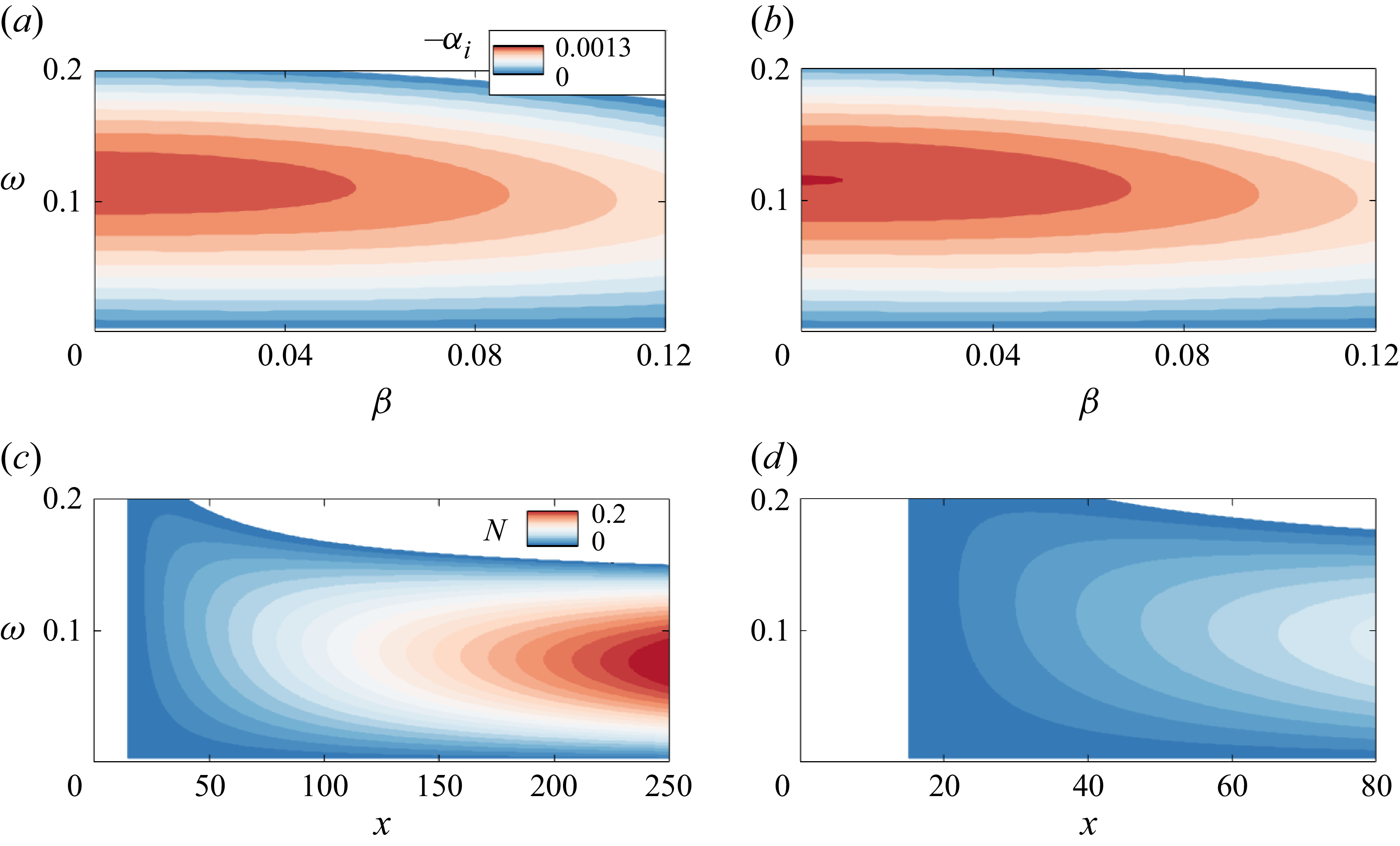
 (a,b)
 −αi
 β
 ω
 x=25
 (c,d)
 N
 x
 ω

 Q

 χ
 a
 ω
 k3=4
 b
 k3
 ω=0

 ω=0
 ϑ=0∘
 k3=4
 k3=16
 p^
 u^
 T^

 a
 Au
 k3
 ω=0
 ϑ=0∘
 k3=4
 b
 d
 Au
 AT
 k3
 ω=0
 ϑ=0∘
 ω
 k3=4
 ϑ=0∘
 ϑ
 ω=0
 k3=4
 x

 Au
 AT
 ω=0
 ϑ=0∘
 k3=4,7.5,10,14,16
 k3

 Q=1.75%
 a
 b
 Au
 AT
 x=146
 c
 f
 Au

 |u^|
 a
 (0,1)
 b
 (0,2)
 c
 (0,0)

 Au
 Q=3.5%
 a
 b

 Q=1.75%
 (a)
 u¯
 (b)
 u¯
 T¯
 x=146
 (c)
 ∂u¯/∂yn
 ∂u¯/∂z
 x=146

 (σd=0)
 Q=1.75%
 x=146
 ω¯i−ω¯r
 α=1,1.8,4
 (d,e)
 α
 ω¯i
 Cr:=(ω¯/α)r
 (f)
 u^SI(yn,z)
 α=1
 ω¯i=0.015

 (σd=0.5)
 Q=1.75%
 x=146
 (a,b)
 α
 ω¯i
 Cr
 (c)
 eiσdk3zu^SI(yn,z)
 α=1
 ω¯i=0.037

 Q=1.75%
 (a)
 u¯
 (b)
 u¯
 T¯
 x=12
 (c)
 ∂u¯/∂yn
 ∂u¯/∂z
 x=12

 Q=1.75%
 x=12
 (a,b)
 α
 ω¯i
 Cr
 (c)
 u^SI(yn,z)
 α=6.4
 ω¯i=0.275

 (σd=0)
 (σd=0.5)
 Q=1.75%
 ω¯
 −αi
 Cr
 N
 −αi<0

 (σd=0)
 (σd=0.5)
 Q=3.5%

 Retr

 a
 pB
 b
 Au
 ω=0
 ϑ=0∘
 k3

 M¯
 (a)
 (b)


