The international relations (IR) literature has long recognized that many of its key variables are relational in nature. Although research has traditionally focused on the dyadic nature of states’ decisions, increasing attention has been paid to how actors’ locations within the global system shape their choices. Most recently, scholars have begun to recast traditional IR variables—such as conflict, trade, alliances, or international organization memberships—as networks connecting international states. Properties of these networks (e.g., density, polarization), and of actor positions within them (e.g., centrality, similarity), may then reveal important insights about international events (e.g., Ward, Hoff and Lofdhall Reference Ward, Hoff and Lofdhall2003; Maoz et al. Reference Maoz, Kuperman, Terris and Talmud2006; Maoz Reference Maoz2010; Cranmer, Desmarais and Menninga Reference Cranmer, Desmarais and Menninga2012). Previous work also recognized the importance of such positional and relational information, as in Signorino and Ritter’s (Reference Signorino and Ritter2002) development of S scores to capture “political affinity” between states. As a result, identifying the relevant properties of international networks and exploring their effects constitutes a large part of research within IR.Footnote 1
There are two general approaches to the construction and use of network measures: measure oriented and estimation oriented. The measure-oriented approach consists of identifying the measure of interest (e.g., centrality, similarity), using the relevant formula to compute the measure, and proceeding to use the resulting measure as a right-hand side variable in a regression. Maoz et al. (Reference Maoz, Kuperman, Terris and Talmud2006), for example, employ this approach to demonstrate that similarities among international states’ positions within the international trade network help explain the occurrence of international conflict. The estimation-oriented approach is theoretically similar, yet more methodologically complex. This approach emphasizes the nonindependence among actors (or nodes) and their relationships (or edges) within a network: for example, if actor A has a direct tie to actor B, and actor B has a direct tie to actor C, then, by construction, actors A and C have an indirect tie between them. These types of network configurations—network configurations that are likely to arise simply by construction—are referred to as “endogenous” network properties. The proponents of the estimation approach maintain that, given a network structure, one cannot properly isolate the effects of the independent variables without properly accounting for the network properties (Cranmer and Desmarais Reference Cranmer and Desmarais2011).
Both approaches provide great leverage in exploring the connection between actors’ positions within networks and actor behavior while accounting for properties endogenous to the network. There exists, however, a different source of network endogeneity that has so far received little attention—endogeneity that may arise as a result of using measures of one feature of the international system to explain another feature. Treating network measures as exogenous to actor behavior, as commonly practiced by the proponents of both approaches, may produce biased estimates if actor positions within networks are in fact endogenous to (not independent of) actor behavior. We examine the use of network measures—such as S scores, structural equivalence (SEq) scores, and degree centrality—as exogenous independent variables when the underlying relational variables used to generate those measures exhibit endogeneity. Although the issue of endogeneity has long been recognized in the study of IR (Reuveny and Kang Reference Reuveny and Kang1996; Keshk, Pollins and Reuveny Reference Keshk, Pollins and Reuveny2004; Hegre, Oneal and Russett Reference Hegre, Oneal and Russett2010), it has not yet become salient among studies using network measures.Footnote 2
For example, what are the implications of including the alliance-based S score in an equation that predicts trade or conflict? As evident from the debate regarding whether alliances lead to more conflict (Lai and Reiter Reference Lai and Reiter2000; Vasquez Reference Vasquez2009), there may be an overlap between the factors that contribute to conflict initiation and those related to alliance formation. Mathematically, the presence of such an overlap may express itself as a correlation between unobserved factors explaining alliances and the conflict outcome—an issue known as endogeneity. This endogeneity may be further exacerbated by using the offending variable to construct a measure of network position similarity, such as S or SEq scores that will then be used to predict an outcome that is endogenous to it. Similar examples may be found in other areas of study, such as the use of trade-based SEq scores to predict conflict, despite the possible endogeneity between conflict and trade. These measures find uses beyond IR, of course, as scholars of American politics have taken similar approaches to examining the influence of Congressional networks on members’ voting patterns (Rogowski and Sinclair Reference Rogowski and Sinclair2012) or success in passing legislation and amendments (Fowler Reference Fowler2006).
We suggest two alternative instrumental variable (IV) approaches for addressing possible endogeneity when employing network-based measures as regressors in subsequent analyses. The first approach—the instrumented network—is to instrument the network itself (i.e., the associated relational variable, such as trade) and then use this instrument to construct the relevant network measure to be used as a regressor. The second approach—instrumented score—retains the network as given and instead generates an instrument of the relevant network score (e.g., instrument trade SEq score), then use the instrumented score as a regressor. Although applying nonlinear functions to possible endogenous variables generally calls for the second approach (Kelejian Reference Kelejian1971), we find that this may not be true for network measures. First, network measures are a special type of nonlinear functions, in which the value for actor i often depends not just on i’s own realization of the variable, but also on the realization of the variable for many, if not all, other actors. Second, network measures usually involve complex functions of the endogenous relational variable that make it hard to identify the correct polynomial from which to directly generate an IV of the measure. We supplement our theoretical argument with Monte Carlo analysis and empirical demonstrations that model (a) the relationship between international trade and conflict networks, (b) inter-state alliances and international trade, and (c) preferential trade agreements (PTA) and economic sanctions, using both naïve and a two-stage IV estimators within the context of standard logit estimators as well as using exponential-family random graph models (ERGMs).
Our results indicate, first, that one should almost never ignore the endogeneity problem as doing so can result in severely biased estimates. Comparing our two corrections, we find that, whereas the instrumented score approach produces slightly less biased estimates, the instrumented network approach produces sufficient gains in precision to be strongly preferred in root mean square error terms. Further, in some cases the bias in the latter can be derived and therefore adjusted for. Finally, the choice of the best correction depends on the network measure at use. We find, for example, that in the presence of moderate to severe endogeneity, the instrumented network approach works best for the use of SEq scores, whereas the instrumented score approach works best for S scores. For the use of centrality, both instrumental approaches are equally preferable to the naïve model.
Measures of Network Position
Along with a new approach to theorizing, network-based approaches have also equipped scholars with a new set of analytical tools that range from new conceptual measures (e.g., centrality, SEq, connectedness) to network-oriented approaches to statistical estimation.Footnote 3 In the current study, we narrow our analysis to three network measures: (1) centrality or degree centrality, which is, perhaps, the most commonly used among the network measures (e.g., see Fowler Reference Fowler2006; Dorussen and Ward Reference Dorussen and Ward2008; Hafner-Burton and Montgomery Reference Hafner-Burton and Montgomery2012; Kinne Reference Kinne2012; Murdie and Davis Reference Murdie and Davis2012); (2) S scores, which are a common measure of relational or political similarity, most frequently applied within the IR subfield (e.g., Stone Reference Stone2002; Bennett and Stam Reference Bennett and Stam2004; Hegre, Maoz Reference Maoz2010; Oneal and Russett Reference Hegre, Oneal and Russett2010); and (3) SEq scores, which have been used as a theoretically similar, yet computationally distinct alternative to S scores (e.g., Snyder and Kick Reference Snyder and Kick1979; Maoz et al. Reference Maoz, Kuperman, Terris and Talmud2006; Hafner-Burton and Montgomery Reference Hafner-Burton and Montgomery2012).
Centrality
The term “network centrality” or “centrality,” for short, refers to a family of network measures, based on the total (sometimes weighted) number of a node’s direct and indirect connections (Bonacich Reference Bonacich1987). In many political science applications, actor centrality is used as a measure of actor power or prestige within the network.Footnote 4 Scholars of IR, for example·, use states’ centrality within the intergovernmental organizational (IGO) network to explain international conflict and economic sanctions (Ingram, Robinson and Busch Reference Ingram, Robinson and Busch2005; Hafner-Burton and Montgomery Reference Hafner-Burton and Montgomery2006; Ward Reference Ward2006; Dorussen and Ward Reference Dorussen and Ward2008; Hafner-Burton and Montgomery Reference Hafner-Burton and Montgomery2008; Hafner-Burton and Montgomery Reference Hafner-Burton and Montgomery2012), or foreign aid allocations (Lin and Shreve Reference Lin and Shreve2013). Others have used centrality to explain the effects of international nongovernmental organizations (Moore, Eng and Daniel Reference Moore, Eng and Daniel2003; Lake and Wong Reference Lake and Wong2009; Carpenter Reference Carpenter2011; Murdie Reference Murdie2014). Scholars of American politics, in the meantime, have used centrality to assess the influence of particular members of Congress (e.g., Fowler Reference Fowler2006).
Following the general trend in the literature, we focus on the measure of degree centrality:
 $${1 \over {\left| V \right|{\minus}1}}\mathop \sum\limits_{j(\ne\,i)} A_{{ij}} ,$$
where V is the set of vertices and A a |V|×|V| adjacency matrix with A ij entries being equal to 1 if an edge connects vertices i and j, and 0 otherwise.
S Scores
Although IR research has offered several alternative measures of political affinity, it is safe to say that various versions of S scores—a spatial measure of policy similarity—developed by Signorino and Ritter (Reference Signorino and Ritter2002) still constitute the state of the art.Footnote 5 The central idea behind the construction of S scores is that one can proxy states’ preferences by using the information from their observable (foreign) policy decisions—referred to as “(foreign) policy portfolios”—on the issues of interest. States with “similar” observable policy decisions will receive similar affinity scores, whereas states exhibiting a lot of policy divergence will be located further away on the affinity spectrum (Signorino and Ritter Reference Signorino and Ritter2002, 126).Footnote 6
More formally, let  $$P^{i} =[p_{1}^{i} ,\,p_{2}^{i} ,\,\,\ldots\,,\,p_{n}^{i} ]$$
represent state i’s policy portfolio on a given issue. Analogously, state j’s policy portfolio on the same issue can be represented by
 $$P^{j} =[p_{1}^{j} ,\,p_{2}^{j} ,\,\,\ldots\,,\,p_{n}^{j} ]$$
. As the observable data represents mappings of states’ policy positions, whereas the true positions are unobservable, Signorino and Ritter introduce a vector L=[l 1, l 2, … , l n] of order-preserving scoring rules
 $l_{k} \,\,\colon\,\,p_{k}^{i} \to{\bf p}_{k} $
, which map data values
 $p_{k}^{i} $
for state i’s policy along dimension k to a value on a closed interval
 $${\bf{p}} _{k} \,\equiv\,\left[ {l_{k}^{{{\rm min}}} ,\,l_{k}^{{{\rm max}}} } \right]\,\subset\,\Re $$
. Finally, let W=[w 1, w 2, … , w n] be a vector of weights.
Signorino and Ritter (Reference Signorino and Ritter2002, 127) define similarity S of states i and j’s policy portfolios P i and P j as follows:
 $$S(P^{i} ,\,P^{j} ,\,W,\,L)={\rm 1}{\minus}{\rm 2}{{d(P^{i} ,\,P^{j} ,\,W,\,L)} \over {d^{{{\rm max}}} (W,\,L)}},$$
where
 $$d\left( {P^{i} ,\,P^{j} ,\,W,\,L} \right)=\mathop \sum\limits_{k=1}^n {{w_{k} } \over {{\rm \Delta }_{k}^{{{\rm max}}} }}\left| {l_{k} \left( {p_{k}^{i} } \right){\minus}l_{k} \left( {p_{k}^{j} } \right)} \right|,$$
and
 $$d^{{{\rm max}}} (W,\,L)=\mathop{\underbrace{{{\rm max}}}}\limits_{X^{i} ,\,X^{j} }d(X^{i} ,\,X^{j} ,\,W,\,L)=\mathop \sum\limits_{k=1}^n {{w_{k} } \over {{\rm \Delta }_{k}^{{{\rm max}}} }}(l_{k}^{{{\rm max}}} {\minus}l_{k}^{{{\rm min}}} )=\mathop \sum\limits_{k=1}^n w_{k} .$$
SEq Scores
Political scientists’ interest in network analysis has also led to the adoption of several alternative measures of relational similarity from sociology. Most prominently, scholars have used the family of measures, knows as the structural equivalence scores (for early uses in sociology, see Boorman and White Reference Boorman and White1976; Burt Reference Burt1976; Sailer Reference Sailer1979). SEq scores is a dyadic measure that captures similarity of network ties between any given actors (nodes) i and j in relation to all other actors (nodes) k in the network. The early applications of SEq scores within the study of IR date back to Brams (Reference Brams1966) and Snyder and Kick (Reference Snyder and Kick1979), whereas more recent research includes Hafner-Burton, Kahler and Montgomery (Reference Hafner-Burton, Kahler and Montgomery2009); Hafner-Burton and Montgomery (Reference Hafner-Burton and Montgomery2012), and Maoz et al. (Reference Maoz, Kuperman, Terris and Talmud2006). The particular type of SEq scores, on which we focus in this paper, is the one used by Maoz et al. (Reference Maoz, Kuperman, Terris and Talmud2006) and calculated asFootnote 7
 $$SEq_{{ij}} ={{\sum \limits_{k=1}^n {\rm (}x_{{ik}} {\minus}\bar{x}_{{{\bullet}i}} {\rm )(}x_{{jk}} {\minus}\bar{x}_{{{\bullet}j}} {\rm )}{\plus}\sum \limits_{k=1}^n {\rm (}x_{{ki}} {\minus}\bar{x}_{{i{\bullet}}} {\rm )(}x_{{kj}} {\minus}\bar{x}_{{j{\bullet}}} {\rm )}} \over {\sqrt {\sum \limits_{k=1}^n {\rm (}x_{{ik}} {\minus}\bar{x}_{{{\bullet}i}} {\rm )}^{2} {\plus}\sum \limits_{k=1}^n {\rm (}x_{{ki}} {\minus}\bar{x}_{{i{\bullet}}} {\rm )}^{2} } \sqrt {\sum \limits_{k=1}^n {\rm (}x_{{jk}} {\minus}\bar{x}_{{{\bullet}j}} {\rm )}^{2} {\plus}\sum \limits_{k=1}^n {\rm (}x_{{kj}} {\minus}\bar{x}_{{j{\bullet}}} {\rm )}^{2} } }},$$
where  $\bar{x}_{{{\bullet}i}} ,\,\bar{x}_{{{\bullet}j}} $
are the respective means of i and j’s exports to every other actor k (row means of the relational matrix X), and
 $$\bar{x}_{{i{\bullet}}} ,\,\bar{x}_{{i{\bullet}}} $$
are the means of the tie strength between k’s and i or j (column means) (Maoz et al. Reference Maoz, Kuperman, Terris and Talmud2006, 674). Note that the first term in the numerator represents the covariance of rows i and j and the second term represents the column covariance, whereas the first term in the denominator represents the sum of the row and column variances for i and the second the same quantity for j. Applying this formula to the network of international exports, Maoz et al. (Reference Maoz, Kuperman, Terris and Talmud2006) argue that the SEq measure gives a sense of the similarity, along the lines of a correlation, of two countries’ outflows and inflows of trade with all other states. In fact, if X is a symmetric matrix, SEq ij is the correlation between X ik and X jk.Footnote 8
Endogeneity of Network Position Measures
Our central argument is that a study of relational variables’ effects is inseparable from the study of network formation. Much like social networks, networks of states rarely form at random—an implicit assumption of using a network measure as an exogenous independent variable in a regression. Instead, both social and international networks emerge in response to two general types of causal effects: homophily—self-selection based on pre-existing similarities—and common exposure (Hays, Kachi and Franzese Reference Hays, Kachi and Franzese2010; Franzese, Hays and Kachi Reference Franzese, Hays and Kachi2012). The difference between these effects is theoretically important: a theory that posits homophily as the causal mechanism behind a network effect must rule out common exposure, and vice versa. Endogeneity of the independent variable can be thought of as a special type of common exposure, whose effect, if present, is especially detrimental for recovering unbiased estimates.
The literature on alliance formation, for example, has shown that the choice of allies may be driven by short- and long-term security prospects (e.g., Morrow Reference Morrow1991), domestic “guns versus butter” trade-offs (Powell Reference Powell1993; Kadera and Morey Reference Kadera and Morey2008), as well as state identity considerations such as regime type (e.g., Lai and Reiter Reference Lai and Reiter2000). These insights, however, are rarely linked to the studies that focus on alliances or related measures (e.g., alliance portfolio similarity) as an independent variable. In the meantime, taking advantage of the insights provided by the alliance formation literature would improve the statistical estimates of alliance effects on such variables as conflict or domestic military spending. In the view of possible endogeneity between alliances and conflict or domestic military spending, estimates would be even further improved by simultaneous or two-stage estimation. Analogously, the trade literature has long pointed to conflict as one of the impediments to the growth and stability of inter-state commercial ties (e.g., Reuveny and Kang Reference Reuveny and Kang1996; Russett and Oneal Reference Russett and Oneal2001; Keshk, Pollins and Reuveny Reference Keshk, Pollins and Reuveny2004; Hegre, Oneal and Russett Reference Hegre, Oneal and Russett2010). A model of a trade network’s effect on conflict could possibly produce more accurate estimates if it accounted for possible endogeneity.
This is not to say, however, that the literature has ignored endogeneity altogether. A number of studies have recognized the issue and attempted to test for it by running “reverse causality” checks or lagging the independent variable (e.g., Pevehouse Reference Pevehouse2002a; Pevehouse 2002Reference Pevehouseb; Pevehouse Reference Pevehouse2005; Maoz Reference Maoz2010). Whether such corrections are sufficient, however, depends on the type and extent of endogeneity (Engle, Hendry and Richard Reference Engle, Hendry and Richard1983; Granato Reference Granato1991). Addressing endogeneity using temporal lags or “reverse causality” may be problematic for several reasons. First, it assumes that a researcher is able to specify the correct lag structure. It is often theoretically unclear how many lags are sufficient to strip the model of endogeneity and defaulting to a one-year lag—the most common fix in the literature—may not be the best solution.Footnote 9 Second, temporal lags are altogether irrelevant in the presence of feedback loops between the independent and the dependent variables (Engle, Hendry and Richard Reference Engle, Hendry and Richard1983; Granato Reference Granato1991).
The issue of network endogeneity has been long recognized (Manski Reference Manski1993). Sociological research, for example, has pointed out the endogeneity between friendship networks and substance abuse (e.g., Snijders, Steglich and Schweinberger Reference Snijders, Steglich and Schweinberger2007; Steglich, Snijders and Pearson Reference Steglich, Snijders and Pearson2010). Taking advantage of the House office lottery, Rogowski and Sinclair (Reference Rogowski and Sinclair2012) conduct an empirical test for an endogenous relationship between congressional office proximity, roll-call behavior and cosponsorship decisions. Within the study of IR, Chyzh (Reference Chyzh2013) models endogeneity between trade network formation and its effect on domestic rule of law using a game-theoretic approach. The bottom line is that the presence of endogeneity remains an empirical issue that is only partially solved by a purely theoretical solution.
IV Approaches for Endogeneity in Network Measures
Social scientists have long known that the presence of endogeneity leads to biased estimates. The primary methodological tool of correcting and accounting for endogeneity in social sciences is the use of IV two-stage estimators, such as two-stage least squares (Gawande and Li Reference Gawande and Li2009; Greene Reference Greene2000). The main idea is that endogeneity is stripped from the “offending” regressors by substituting a set of “instruments”—exogenous variables that are correlated with possibly endogenous regressors, yet not affected by the dependent variable.
In its simplest form, endogeneity is defined in the following way. Let us start with the model
 $$Y=X\beta {\plus}\epsilon ,$$
where Y is the dependent variable, X the independent variable, β the coefficient on X, and ϵ the error term. To say that X is an endogenous regressor simply means that there is a non-zero correlation between X and . As a result, a random shock to the dependent variable Y leads to a change in X. In order to identify β, we substitute the endogenous regressor X with a set of exogenous regressors Z that predict it
 $$X=Z\gamma {\plus}\upsilon ,$$
where Z is uncorrelated with the error terms υ and ε, which makes it exogenous to the model.
In our context, we need a little more structure to describe endogeneity. As we construct the potentially endogenous regressor from an observed variable, not necessarily included in the regression equation of interest, it is not the regressor itself that may be endogenous but rather the variable from which we create it. Thus, we can describe our equation of interest as
 $$Y_{{ij}} =X_{{ij}} \beta {\plus}S_{{ij}} \delta {\plus}\epsilon _{{ij}} ,$$
where S ij represents a network measure of the location of units i and j based on some relational variable R ij. Note that we have moved to an explicitly dyadic context here as these models generally focus on how two units’ relative locations affect a joint outcome between them.
We introduce possible endogeneity through R ij
 $$R_{{ij}} =Z_{{ij}} \gamma {\plus}\eta _{{ij}} ,$$
by allowing for non-zero correlation in the joint distribution of the error terms:
 $$\left( {\matrix{ {{\epsilon}_{{ij}} } \hfill \cr {\eta _{{ij}} } \hfill \cr } } \right)\,\sim\,{\rm BVN}\left( {\left( {\matrix{ 0 \hfill \cr 0 \hfill \cr } } \right),\left[ {\matrix{ {\sigma _{1}^{2} } \hfill & {\sigma _{{12}} } \hfill \cr {\sigma _{{12}} } \hfill & {\sigma _{2}^{2} } \hfill \cr } } \right]} \right).$$
As a proof of bias caused by endogeneity would depend on the precise formula used to calculate a particular network measure, S ij (and may or may not exist depending on exactly how such a measure is created) we leave that for studies of specific measures and provide illustrations of potential bias in our Monte Carlo analysis. Of interest will be whether differences across the formulas for the network measures lead to different amounts of bias when the relational variable exhibits endogeneity. First, we outline two distinct approaches to addressing the problem.
IV of the Network Score/Measure
Our first approach, which we hereafter refer to as the instrumented score approach, follows the standard IV implementation in which we generate an instrument for S ij using a linear regression model. Of course, as we calculate S ij from the relational variable R ij and the possible endogeneity enters through the latter, we do not face the standard IV setup with two linear equations. Rather, our possibly endogenous regressor depends in a nonlinear way on the endogenous variable R ij. We therefore turn to the work of Kelejian (Reference Kelejian1971) on the inclusion of nonlinear functions of endogenous variables. Following its approach, our Equation 8 may be estimated consistently if we can find an instrument for S ij that is uncorrelated with and linearly independent of X ij.
To generate the instrument, note that we can write the expectation of S ij as a function of the fixed variables Z ij and an unrelated random error. Kelejian (Reference Kelejian1971) then shows that even though we may not know the exact form of this function we can approximate it with the OLS prediction,  $$\widehat{S}_{{ij}} $$
, that results from regressing S ij on a polynomial in Z ij of degree d. For large enough d, Z ij and
 $$\widehat{S}_{{ij}} $$
are linearly independent, which results in consistent estimates. Note that the elements of Z ij may be identical to those of X ij as Kelejian (Reference Kelejian1971) assumes in his exposition.
The unknown here involves picking a large enough d to insure independence of X ij and the instrument. An additional complication in our setting arises from the fact that  $$\widehat{S}_{{ij}} $$
often depends on the value of the exogenous variables, Z for units i and j, but also on their values for all other units. Most obviously, the calculation of the SEq score for just one pair ij involves the values of R kl for all other pairs kl. Thus, the best linear approximation to S ij may depend on polynomials of the values of Z for all units, which may undermine our ability to generate a valid instrument through the IV equation as described above.
Instrumenting the Network
Our second approach, which we call the instrumented network approach for short, parallels the standard IV solution but adds the extra step of generating the appropriate relational measure from an instrument. Thus, we estimate the regression model corresponding to Equation 9, generate predicted values  $$\widehat{R}_{{ij}} $$
and construct the network score from these values, which we refer to as
 $$S_{{ij}} (\widehat{R}_{{ij}} )\,\equiv\,\widehat{S}_{{ij}} $$
. We then substitute the instrumented relational score,
 $$\widehat{S}_{{ij}} $$
, into our estimation of Equation 8:
 $$Y_{{ij}} =X_{{ij}} \beta {\plus}\widehat{S}_{{ij}} \delta {\plus}\epsilon _{{ij}} .$$
Two items warrant further discussion at this point. First, because we are using an estimated instrument, our standard errors will tend to be too small. The usual solution is either to estimate the two stages simultaneously or to correct the standard errors after estimation. Given that the first solution is rather involved in the presence of a nonlinear function of the instrumented variable, and also given that our goal is to develop a solution for arbitrary network measures, we utilize a re-sampling approach. Specifically, we take draws of the estimated distribution of  $$\widehat{R}_{{ij}} $$
, calculate the resulting network measure
 $$S_{{ij}} (\widehat{R}_{{ij}} )$$
, and average across the resulting estimates to obtain correct standard errors according to Little and Rubin’s (Reference Little and Rubin2002) formula for multiply imputed data.Footnote 10
Second, the nonlinearity of  $$S_{{ij}} (\widehat{R}_{{ij}} )$$
means that
 $$E[\widehat{\delta }\!\mid\!S_{{ij}} (\widehat{R}_{{ij}} )]=\delta $$
may not hold. As Kelejian (Reference Kelejian1971) proves, this approach will generally produce an inconsistent estimate of δ.Footnote 11 As our instrument removes the error terms in the relational equation and calculates the network measure using the explained portion, we will effectively increase the correlation (and therefore the network measure). Put differently, the correlation between two variables with stochastic errors added is smaller than without it. This change in the scale of S ij will affect the estimated coefficient.Footnote 12 In the example just given, the estimate will be smaller than δ, as this would allow the estimator to “preserve” the correct marginal effect of S ij. Possible concerns about the effectiveness of the two alternate IV methods warrant a comparison, which we present in the remainder of the manuscript.
Monte Carlo Analysis
In order to investigate the effects of endogeneity in variables used to create network measures, we performed a Monte Carlo analysis using a data generation process designed to mimic what one might find in a typical political science study. We start by generating information about 100 units. We then create a dyadic version of these data in order to generate relationship data between these units. Next, we use this information to generate network measures based on units’ relational data, as well as an outcome variable that depends on those relationships. In order to investigate the effects of relational endogeneity, we introduce varying amounts of correlation between the relational data and the outcome of interest.
Monte Carlo Setup
More formally, we start with a list of i=1, 2, … , n units with characteristics captured by variables X i and Z i, both of which have a standard normal distribution. We then create a dyadic data set consisting of all pairwise combinations of units, totaling 10,000 observations from which we omit the same unit dyads, leading to a final sample size of 9900.
To generate interesting network scores, S ij, we place each country in a common space and let the relational variable, R ij, depend on i and j’s relative location in this space. Specifically, we evenly space each unit across a 10×10 grid and calculate the Euclidean distance, d ij, between the two units in each dyad. We then generate our relational variable based on the unit-specific characteristics and distance:
 $$R_{{ij}} =Z_{{{\rm 1}i}} {\plus}Z_{{{\rm 1}j}} {\minus}d_{{ij}} {\plus}\eta _{{ij}} ,$$
where the error terms are i.i.d. standard normal. Including distance in this equation makes it so that units near each other will have common patterns in their values of R ij, which will create similarity among nearby pairs and dissimilarity among pairs that are further away. To maintain comparability between variable scales, we normalize the standard deviation of the distance variable to 1. We then use the observed outcomes for R ij to create our network measure, S ij. Here we consider three such measures: centrality, S scores, and SEq as in Equations 1, 2, and 5.
For each dyad we then calculate the outcome variable of interest as a linear regression equation:
 $$Y_{{ij}} =0.25{\times}X_{{1i}} {\plus}0.25{\times}X_{{1i}} {\plus}\delta {\times}S_{{ij}} {\minus}0.25{\times}d_{{ij}} {\plus}\epsilon _{{ij}} ,$$
where X 1k indicates the value of variable X 1 for country k in the dyad, S ij the network score for units i and j, and d ij the Euclidean distance between the two states.Footnote 13 The error term is generated from a standard normal. The coefficient on the network score changes depending on which one we use as they each have different scales: for SEq we set δ=−1, for S scores δ=−2.5, and for centrality δ=−0.2.
In order to ascertain the effects of endogeneity, we then introduce correlation between the two error terms by drawing them from a bivariate normal distribution:
 $$\left( {\matrix{ {{\epsilon}_{{ij}} } \hfill \cr {\eta _{{ij}} } \hfill \cr } } \right)\,\sim\,\rm BVN\left( {\left( {\matrix{ 0 \hfill \cr 0 \hfill \cr } } \right),\left[ {\matrix{ {\sigma _{1}^{2} } & {\sigma _{{12}} } \cr {\sigma _{{12}} } & {\sigma _{2}^{2} } \cr } } \right]} \right).$$
We set the variances equal to 1, which means that the covariance equals the correlation, which we vary from −0.75 to 0.75 by increments of 0.25. For each value we generate 500 draws of the error terms, calculate the outcome, relational variable, and network measures, and then estimate the coefficients in Equation 13 through linear regression. Although we focus here on a continuous outcome variable, note that similar results are obtained for a dichotomous variable representing a network tie estimated with an ERGM.
Finally, in order to correct for the possible endogeneity of S ij we consider both approaches discussed above. First, we instrument the relational variable, R ij, by estimating Equation 12 via linear regression, calculating its predicted value,  $$\widehat{R}_{{ij}} $$
, then constructing the network measures using the instrument (e.g.,
 $$\widehat{S}_{{ij}} =SEq(\widehat{R}_{{ij}} )$$
) and using these instrumented scores when we run the regression corresponding to Equation 13. We repeat this five times with draws from the estimated distribution of
 $$\widehat{R}_{{ij}} $$
to capture the uncertainty in our instrument. Second, we directly create an instrument of the score, S ij, by estimating a linear regression that includes third-order polynomials in Z i and Z j; a third-order polynomial in the product of Z i and Z j; and the products of distance with Z i, Z j, and Z iZ j.Footnote 14 We hope to capture the complex dependence of S ij on the exogeneous variables in the equation for R ij. Examining the results for single draws indicated that adding these variables improved our ability to predict S ij. For the simulation using SEq scores we transform the score generated from the instrumented network to put it on the same scale as the original variable.Footnote 15
Monte Carlo Results
We present the results of our Monte Carlo analysis graphically in Figure 1. Tables with more complete details are available in our supplemental appendix. The top plot shows the average estimate and a 95 percent band around it (based on the standard deviation of the sampling distribution) across the 500 draws for each value of ρ, whereas the bottom plot shows the average estimates of the coefficients for X 1i and X 1j. The latter show no bias whatsoever, which is not surprising given that these variables have no correlation with the information in the SEq score, so we focus our discussion on the coefficient for the SEq variable.
Monte Carlo results for average coefficient estimates for network measures and distance variable in the equation of interest, varying error correlation. Note: Uncorrected models use the observed value of Rij to calculate the network score, Sij(Rij). Score of instrumental variable (IV) models use an estimate of Rij from a linear regression to generate  $$S_{{ij}} (\widehat{R}_{{ij}} )$$
. IV of score models runs an IV regression that models Sij(Rij) with a linear regression (see text for details). Results are based on 500 draws for each value of ρ. Confidence intervals are calculated using the standard deviation of the sampling distribution of the coefficient estimates. True values are indicated by darker lines.

The Monte Carlo results show clear evidence of bias for this variable. The line denoted with circles represents the naïve, or uncorrected model, in which the network measures are constructed using the observed relational variable, that is, S ij(R ij). The naïve model shows a negative bias with a negative correlation between the error terms in the relational and outcome equations and an upward bias with a positive correlation. The endogeneity appears to create bias by increasing the relational variable, whereas simultaneously increasing the outcome of interest, Y ij. That is, units appear to be more or less similar than they should be, based on the sign of the correlation between the unobserved components of the relational and outcome variables. The extent of the apparent bias makes it so that the 95 percent confidence interval does not even include the true value for greater degrees of correlation. Note that a correlation of 0 breaks this dependence and results in an unbiased estimate.
The line denoted by triangles shows the results for the network measure calculated on the instrumented network model, that is,  $S_{{ij}} (\widehat{R}_{{ij}} )$
. As noted above we adjusted this variable to account for the difference in scale that results from our instrument compared with the observed relational variable. This adjustment clearly works as the resulting average estimate sits quite close to the true value. Finally, the line denoted by squares presents the results for the instrumented score model using
 $\widehat{S}_{{ij}} $
. The model again estimates the true coefficient spot on, although its confidence interval is noticeably larger than those for the two previous models. These results therefore point to the instrumented network approach as superior on root mean squared error terms.
Next, we evaluate the results for S scores, generated using the same procedure. Overall, these results mirror those for the SEq score, but some differences emerge. The apparent bias in the coefficient on the S score appears to be smaller in an absolute sense and also with respect to the variation of the estimates. Although the average estimate differs by as much as 20 percent, the 95 percent central region of the sampling distribution always includes the true value of 0.5. The results for the instrumented network approach show no dependence on the correlation, but deviate from the true value by a constant amount. We believe that this result occurs owing to a change in the variation of the underlying variables when calculated using the instrumented rather than the observed relational variable. In this case a correction is not as straightforward as it was for SEq. The instrumented score approach for S scores is again spot on the true value of the coefficient. Just as with the SEq estimate, the confidence interval also appears only somewhat larger than that estimated by the instrumented score model, although the difference is not that stark, and given the bias the instrumented score approach outperforms the instrumented network approach in root mean squared error terms.
The last plot in the first row of Figure 1 presents the analogous results for an analysis using centrality scores. The estimates of the uncorrected model again exhibit a negative bias for a negative error correlation and a positive bias for a positive error correlation, albeit the 95 percent confidence interval does contain the true value. The estimates of both IV models, in the meantime, are effective at correcting the bias and capturing the true values. Unlike in the previous two applications, the confidence intervals produced by the two IV models closely overlap, producing no clear winner in root mean squared error terms.
The bottom row of Figure 1 reports the estimates for the distance variable. This allows us to determine whether the estimated coefficients for variables in both equations are affected by endogeneity. In the case of the SEq measure, the plot supports our expectation by showing deviations in the average estimate for the coefficient on distance in the uncorrected model. The apparent bias in the former represents about 20 percent of the true value and the 95 percent confidence bands only overlap the true value when the correlation is near 0. The instrumented network model seems to perform the best, providing an apparently unbiased estimate of the true coefficient. The instrumented score approach captures the true value of the coefficient, yet produces a larger confidence interval. The S score and centrality applications reveal fewer noticeable differences among the three models, with both the estimates and the confidence intervals nearly perfectly overlapping.
Overall, then, our Monte Carlo results show that endogeneity in relational variables used to construct network-based or other relational measures can lead to bias in the estimated coefficient on the network measure variable. This apparent bias increases with the absolute value of the correlation between the error terms in the two equations. The deviations may be sufficiently large to wash out the effect of the network measure or even to result in incorrectly signed coefficients. Further, the endogeneity bias can also infect other variables that appear in both equations (and we speculate that it would affect any variable in the outcome equation correlated with variables in the relational equation). Either of two IV corrections we propose appears to eliminate endogeneity bias in the coefficients for variables that appear in both equations, though changes in the scale of the underlying variable can result in constant deviations from the true value as shown in the case of S scores.
Empirical Applications
We demonstrate the advantages of the two-stage IV approaches to correcting endogeneity in network measures with three empirical examples. The first two applications draw from the study of conflict and trade. This relationship has been of perennial interest to scholars with a great deal of attention recently to boundary conditions and endogeneity (e.g., Reuveny and Kang Reference Reuveny and Kang1996; Keshk, Pollins and Reuveny Reference Keshk, Pollins and Reuveny2004; Hegre, Oneal and Russett Reference Hegre, Oneal and Russett2010; Lu and Thies Reference Lu and Thies2010; Peterson and Thies Reference Peterson and Thies2012). The dominant argument in contemporary scholarship holds that economic interdependence decreases conflict because conflict is associated with increased investment risks, increased transaction costs, interruptions to the flow of information, and otherwise leads to economic losses (Russett and Oneal Reference Russett and Oneal2001; Gartzke Reference Gartzke2007).Footnote 16 The reverse argument avers that, rather than trade reducing conflict, conflict reduces trade owing to the “primacy of politics” over economics. According to this argument, firms and investors tend to “follow the flag” and are unwilling to do business in politically hostile countries (Keshk, Pollins and Reuveny Reference Keshk, Pollins and Reuveny2004). Multiple empirical tests of the trade–conflict relationship, including simultaneous estimation, provide support for both arguments, suggesting that the relationship is endogenous. We explore this endogenous relationship by replicating Maoz et al. (Reference Maoz, Kuperman, Terris and Talmud2006), Cranmer and Desmarais (Reference Cranmer and Desmarais2011), and Long (Reference Long2008). The first two studies examine how trade SEq scores affect conflict, whereas the third includes alliance similarity when predicting bilateral trade flows.
Our third empirical application explores the relationship between states’ centrality within the network of PTAs and economic sanctions. Although states with powerful positions within the PTA network may be more likely to issue economic sanctions, position within the PTA network may be endogenous to the ability and willingness to issue sanctions in the first place. To investigate this relationship, we conduct a replication of Hafner-Burton and Montgomery (Reference Hafner-Burton and Montgomery2008), who make the former argument.
SEq Scores: Trade–Conflict Endogeneity
Our first empirical demonstration is based on recent work by Maoz et al. (Reference Maoz, Kuperman, Terris and Talmud2006), who have imported the trade–conflict argument into a networks framework. Treating both inter-state trade and conflict as networks with states representing nodes, Maoz et al. (Reference Maoz, Kuperman, Terris and Talmud2006) demonstrate support for the pacifying effect of trade SEq, or SEq within the international trade network. The literature suggests, however, that trade and conflict may be endogenous to each other, that is, ongoing or anticipated conflict may reduce trade flows (Keshk, Pollins and Reuveny Reference Keshk, Pollins and Reuveny2004). This means that we may expect an error correlation between trade—the relational variable used to construct SEq scores—and conflict—the dependent variable. More formally, the error η ij in the relational covariate trade (R ij) may be correlated with the error ϵij in the dependent variable, conflict (Y ij).
In order to explore the advantages of the IV two-stage estimation, we use the two approaches discussed above to re-estimate Maoz et al. (Reference Maoz, Kuperman, Terris and Talmud2006) on a sample of all dyads between 1961 and 1996. In our analysis, we pay particular attention to the relationship between trade SEq and conflict.
The first approach—instrumented network—is to construct predicted values  $\widehat{{R_{{ij}} }}$
for A–B bilateral exports using a linear regression, and then use these predicted values instead of the observed values of exports, R ij, to construct the trade SEq variable,
 $\widehat{{S_{{ij}} }}$
, which we will substitute into the outcome equation of conflict, Y ij. The second approach—instrumented score—is to construct an instrument of the trade SEq score itself to subsequently use in the outcome equation of conflict, Y ij. Standard errors for the second stage of the model are obtained by repeating the following steps five times: re-sample the trade instrument from its estimated distribution, recalculate the SEq scores, and estimate the model. We then average the results according to Little and Rubin’s (Reference Little and Rubin2002) formula for multiply imputed data as described previously.
Trade instrument
The IV for exports between A and B is constructed based on the gravity model of trade (Hegre Reference Hegre2009; Hegre, Oneal and Russett Reference Hegre, Oneal and Russett2010). It includes the distance between the two states, as well as their gross domestic product (GDP) and population. In addition to these components of the gravity model, trade between two states may depend on each state’s resource endowment. States rich in such highly desired resources as oil and natural gas, may have larger export volumes of these commodities. The literature also suggests, however, that oil-rich states may have lower overall export volumes, as over-reliance on raw commodities may lead to a lack of development in other sectors (Sachs and Warner Reference Sachs and Warner2001). The data on GDP and population is obtained from the Expanded Trade and GDP data (Gleditsch Reference Gleditsch2002), whereas resource endowment is measured as natural gas and oil endowment using data collected by Ross (Reference Ross2011). Unfortunately, economic data often suffers from a large number of missing values and imprecision, especially as one goes farther back temporally. In addition, resource data is unavailable before 1961 and after 1996. Therefore, we limit our analysis to 1962–1996 (due to a one-year lag). Finally, we log all variables to control for skewness. We add 0.001 to the trade variable in order to maintain as many observations as possible. As every observation is used to calculate the SEq scores, losing even a small number is problematic.
We report the results of the model used to create the trade instrument in our supplemental appendix in Table 7. We use the predicted export values to construct the corrected export SEq scores to use in the second stage of estimation.Footnote 17 In doing so, we closely follow Maoz et al.’s (Reference Maoz, Kuperman, Terris and Talmud2006) procedure: we start by exponentiating the logged predicted values, then reshape the dyadic data into an n×n matrix, whose ij cell entries represent the predicted export values divided by GDP, and whose diagonal entries are defined as 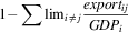 $1{\minus}\mathop{\sum}{{\rm lim}_{{i\,\ne\,j}} {{export_{{ij}} } \over {GDP_{i} }}} $
. Finally, we use the resulting matrix to calculate the export SEq or trade SEq, using the formula in Equation 5.Footnote 18
The conflict equation
The values of the dependent variable in the second stage—conflict—are coded as 1 if i and j experienced a military inter-state dispute (MID) in a given year, and 0 otherwise. The estimation sample includes the total of 166 states between 1961 and 1996.
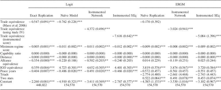
Following Maoz et al. (Reference Maoz, Kuperman, Terris and Talmud2006), in addition to trade SEq, we regress the MID variable on distance, capability ratio, minimum regime score, alliance SEq, IGO SEq, and peace years. For the exact replication, we also use the temporal splines included in the replication data. In all other models, we substitute splines with a linear, quadratic, and cubic polynomials of time (Carter and Signorino Reference Carter and Signorino2010), as the manuscript does not include the information on the knots chosen for the splines. Alliance SEq and IGO SEq are calculated analogously to the trade SEq variable, albeit without our correction for endogeneity.Footnote 19 For spatial considerations, we refer the reader to Maoz et al. (Reference Maoz, Kuperman, Terris and Talmud2006) for detailed information on the coding and data sources for these variables.
Table 1 presents the results of our replications and analyses. Model 1 or exact replication is a straight replication of Model 2 of Table 2 from Maoz et al. (Reference Maoz, Kuperman, Terris and Talmud2006)—the authors’ main model of results.Footnote 20 Model 2 or naïve model presents our replication of the same model, albeit restricted to the estimation sample from our IV equation (Table 7 in supplemental appendix).Footnote 21 Although the dramatic decrease in sample size (and the associated loss in statistical power) results in some differences in terms of statistical significance (on distance and alliance SEq), the main inferences are unchanged. All of the statistically significant coefficients are signed in the same direction as in Model 1.
Exploring Endogeneity in SEq Scores. Replication and extension of Maoz et al. (Reference Maoz, Kuperman, Terris and Talmud2006)
Note: Exact replication re-estimates Model 2 of Table 2 (all dyads, 1816–2000), using the replication data made available by Maoz et al. (Reference Maoz, Kuperman, Terris and Talmud2006). All variables are lagged one period. Sample size differences between exact replication and other models are due to data availability on the variables used for constructing instrumental variables; they cover the period 1962–1996. Just like in the original study, all independent variables are lagged one year. The correlation between the trade SEq variable in the naïve model and instrumented network model is 0.31, whereas that between the naïve model and instrumented SEq model is 0.23. The exact and naïve models employ the same trade SEq variable. Variables capturing spline (Model 1) and cubic time trends (Models 2–6) are included but not reported.
ERGM=exponential-family random graph models; IV=instrumental variable; IGO=intergovernmental organization.
*p<0.05, **p<0.01.
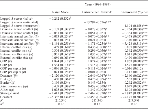
The Issue of Endogeneity in S Scores. Replication and Extension of Long (Reference Long2008)
Note: Naïve model is the exact replication of Long (Reference Long2008, Table 1). The data were made available by the author. The correlation between the logged S scores variable in the naïve model and instrumented network model is 0.37, whereas that between the naïve model and instrumented S score model is 0.61. The exact and naïve models employ the same logged S scores variable.
GDP=gross domestic product; PTA=preferential trade agreements.
†p<0.1, *p<0.05, **p<0.01, ***p<0.001.
Models 3 and 4 present the results of re-estimating the same model using the instrumented network and the instrumented score approaches, accordingly. Finally, given the growing attention to network-oriented estimation approaches, such as ERGMs (for a detailed description, see Cranmer and Desmarais Reference Cranmer and Desmarais2011), we estimated Models 5–7 using the same specifications, but as an ERGM rather than a logistic regression. Both logistic regressions and ERGMs produce a similar pattern of results: in both of the naïve models, the coefficient on trade SEq is many times smaller in magnitude (and statistically insignificant in the ERGM) than in the IV models.
This pattern of results becomes clearer in the view of the above Monte Carlo analysis.Footnote 22 Specifically, the Monte Carlo analysis has demonstrated that there may be a divergence in results between the naïve and either of the IV models, in the presence of high endogeneity. A high positive error correlation between the relational variable and the dependent variable results in an upward bias in the coefficient on the SEq variable in the naïve model. Analogously, a high negative error correlation produces a downward bias. Both the IV models, in the meantime, are virtually unbiased, although the instrumented network model typically produces smaller standard errors.
Of course, the findings of the Monte Carlo analysis apply to “textbook-perfect” research conditions that are rarely met when working with real empirical applications. Thus, for example, unlike the results of the Monte Carlo, the models presented in Table 2 are not fully comparable: Models 1, 2, and 4 use trade SEq scores that are calculated from all available trade data for the time period, whereas in Model 3 the calculation of trade SEq is limited to the estimation sample from the instrument model (Table 1). In light of the SEq scores’ sensitivity to the treatment of missing values, which we uncovered in the course of our analyses, the results in Model 3 are not directly comparable with Models 1, 2, and 4.Footnote 23
With this in mind, the pattern of results presented in Table 1 could be tentatively explained by a high positive error correlation between trade and conflict.Footnote 24 Such an error correlation would cause attenuation bias on the trade SEq coefficient in the naïve model, whereas both of the IV models would recover the unbiased coefficient of larger absolute value.
The four models also exhibit some variation in statistical significance among the coefficients on other variables. In particular, alliance SEq is statistically insignificant in the naïve model, but becomes significant in the instrumented network model (though remains insignificant in the ERGMs). Similarly, the coefficient on distance, whereas statistically insignificant in the naïve model, becomes statistically significant in both the logit and ERGM instrumented score models. For alliance SEq, in particular, these inconsistencies could stem from the endogeneity issue, analogous to that explored here using the example of trade SEq: the network of international alliances may not be independent of that of conflict.
The broad take-away point of the results presented in Table 1 is that the use of SEq scores in the presence of high error correlation may result in substantive bias in the estimates. The suggested IV models may help diagnose such error correlation and make the necessary adjustments in the interpretation and use of the results.
S Scores: Alliance–Trade Endogeneity
Our second example draws on the work by Long (Reference Long2008), who argues that bilateral trade decreases in anticipation of conflict, as looming conflict is an indication of an upcoming spike in the costs of transportation, transaction, and production. Long’s theoretical model includes a set of additional covariates of bilateral trade, including the strength of diplomatic ties. Arguing that states with good diplomatic relations may engage in greater levels of trade, Long (Reference Long2008) includes this effect in the empirical model, operationalizing diplomatic relations as dyad-specific weighted S scores of alliance portfolios. A possible issue here is that state A’s choice of trade partners may be nonindependent from its alliance commitments: relative security concerns, for example, may dictate that states trade within rather than outside of their security alliances (Gowa Reference Gowa1995). As a result, there may be an error correlation between bilateral alliances—the variable used to construct S scores—and A–B bilateral trade—the dependent variable. We explore this issue by re-estimating the empirical analysis of Long (Reference Long2008) using the two IV approaches proposed above.
The first approach—instrumented network—is to construct predicted values  $$\widehat{{R_{{ij}} }}$$
for A–B bilateral alliance using a linear regression, and then use these predicted values instead of the observed values of alliances, R ij, to construct weighted alliance S scores,
 $\widehat{{S_{{ij}} }}$
, which we will plug into the outcome equation of trade, Y ij. The second approach—instrumented score—is to construct an instrument of the S score itself to subsequently use in the outcome equation of trade, Y ij.
Alliance instrument
Along with most of the IR literature, Long (Reference Long2008) obtains the data on weighted S scores from the EUGene program (Bennett and Stam Reference Bennett and Stam2000). Generating predicted S scores to replicate Long (Reference Long2008), therefore, requires that we also follow the same procedure of calculating S scores from the EUGene data. These S scores are based on the alliance type variable, obtained from the Alliance Treaties Obligations and Provisions data set (Leeds et al. Reference Leeds, Ritter, Mitchell and Long2002) and state capability index variable from the Correlates of War (COW) data set (Singer Reference Singer1987). The alliance type variable is treated as an ordinal measure, with the value of 0 representing the absence of an alliance, 1 representing an entente, 2 representing a neutrality pact, and 3 representing a defense pact between states A and B in a given year (Signorino and Ritter Reference Signorino and Ritter2002). Self-dyads of the type i—i are commonly assigned the value of 3 (Sweeney and Keshk Reference Sweeney and Keshk2005), following the logic that a state will defend itself if attacked (Bueno de Mesquita Reference Bueno de Mesquita1975).
To construct the instrument, we regress this variable on a set of covariates associated with alliance formation, relying on the alliance formation equation from Long, Nordstrom and Baek (Reference Long, Nordstrom and Baek2007). The results of the model used to create the instrument are presented in Table 8 of our supplemental appendix. The model shows that stronger alliance commitments are found between states of similar regime type as well as strategic rivals and states with a greater number of total allies. The strength of alliance commitments is negatively affected by distance, major power status and external threat.
Next, we utilize the predicted values to generate the S score instrument using Equation 2. Consistent with Long (Reference Long2008), we weight predicted alliance portfolios by Side B material capabilities, obtained from the COW data set (Singer Reference Singer1987). Despite the difference, the raw and the corrected measures still have a rather high correlation of r=0.45. Mimicking Long (Reference Long2008), we proceed to log our instrumented S scores before using them as a regressor in the trade equation.Footnote 25
Trade equation
Next, we re-estimate Long (Reference Long2008) using the author’s replication data. The side-by-side results of the naïve and the corrected models are presented in Table 2. Model 1 displays the results of the naïve model, Model 2 presents the results of the model, in which we first create an instrument of alliance, use this instrument to calculate the corrected S scores, and substitute these S scores in the original equation. The third model (instrumented S score) displays the results from a standard IV regression with S scores as the endogenous variable.
The side-by-side comparison of results reveals several indications of endogeneity and associated bias in the naïve model. First, note the difference between the coefficients on the estimated and naïve S score variable: insignificant in the naïve model, this coefficient is both significant and substantially larger in absolute value in both of the corrected models, albeit the coefficient in the instrumented network model is the smallest in value (−13.294 compared with −1.194 in the instrumented S score model). Unlike the naïve model, both of the corrected models suggest some evidence of a negative relationship between alliance portfolio similarity and trade.
We can further explore these results, in the view of the findings from our Monte Carlo analysis. In particular, the Monte Carlo analysis shows that the results of the naïve model may diverge from those of the two IV models in the presence of strong endogeneity between the relational variable and the outcome variable. A strong positive error correlation leads to a positive bias in the coefficient on S scores, whereas a strong negative correlation leads to a negative bias. We also demonstrated that the instrumented network approach will be characterized by downward bias in the S score coefficient, whereas the instrumented score approach will produce an unbiased estimate.
Judging from the patterns of results presented in Table 2, we may then suspect a positive error correlation between alliance and trade, that is, states that have a lot of overlap in their allies also engage in more trade. More broadly, the divergence in results between the three models indicates endogeneity between the relational and the outcome variables. Just as with the SEq scores, our recommendation is to explore rather than ignore the issue by estimating both of the IV models we suggest. Such additional analyses will serve as a robustness check for the main results and allow for uncovering possible endogeneity.
Centrality: PTA-Sanctions Endogeneity
Our final empirical application is a replication of Hafner-Burton and Montgomery (Reference Hafner-Burton and Montgomery2008), who demonstrate that states with high centrality in the PTA network are most likely to issue economic sanctions. In this example, we would like to draw attention to the possible nonrandom formation of the PTA network and its possible endogeneity with respect to the sanctioning behavior. Imposing economic sanctions is a form of conflictual behavior, albeit of lower level than a military dispute. Conflictual behavior between two states may affect their trade relationship, such as whether they sign a PTA. Just like with previous empirical applications, we proceed in two stages. First, we use a set of regressors to predict whether two states are likely to be part of a PTA, which allows us to construct predicted values  $\widehat{{R_{{ij}} }}$
for the number of shared PTA memberships between pairs of states. We then use these predicted values to construct PTA centrality scores for each state in the system, which we proceed to use instead of the “uncorrected” centrality scores in Hafner-Burton and Montgomery’s (Reference Hafner-Burton and Montgomery2008) model of economic sanctions. Second, we construct a direct instrument of PTA centrality itself, and use this in the outcome equation of economic sanctions.
PTA instrument
Magee’s (Reference Magee2003) study of bilateral PTA agreement formation provides a great guide for identifying the necessary regressors for our PTA instrument. First, we include an indicator variable of joint membership in the General Agreement for Tariffs and Trade (GATT) or World Trade Organization (WTO) in the previous year with the expectation that states with joint GATT/WTO memberships are likely to have worked out additional bilateral trade agreements whether simultaneously or as a result of their negotiations under GATT. Second, it is important to account for the size of both parties, as we know that larger states constitute more attractive trade partners, especially for states with smaller markets (Hegre, Oneal and Russett Reference Hegre, Oneal and Russett2010). We accomplish this by including lagged values of each state’s logged GDP per capita, as well as a variable that equals to the logged difference between the two states’ GDP per capita. As trade tends to decline with distance, we also include a variable that measures the logged distance between the two states as well as an indicator variable, contiguity, that captures whether the two states share a border.
Next, states might be more likely to enter in a PTA if they already share alliance ties. We capture this by including an indicator variable, allies, that captures whether the two states are part to an alliance. We may also suspect that states may be more likely to enter a PTA if the majorities of their populations speak the same language. We control for this by including a binary indicator same language. We also know that democratic states tend to engage in more trade than dyads made up of autocracies or mixed in terms of regime types (Hegre, Oneal and Russett Reference Hegre, Oneal and Russett2010). We account for this by including an indicator variable that captures joint democracy. Two states may also be more likely to form a PTA if they already view each other as major trade partners. We account for this by including a lagged value of bilateral trade. Finally, the network of international PTAs has been shown to exhibit the tendency toward triadic closure, i.e. states A and B are more likely to form a PTA with each other if both A and B are already part to a PTA with the same state C (Manger, Pickup and Snijders Reference Manger, Pickup and Snijders2012). We account for this network dynamic by including a triadic closure variable, coded as 1 if states A and B share an “indirect” PTA link by both sharing at least one PTA with the same state C, and 0 otherwise.
The resulting model is presented in Table 9 of our supplemental appendix. Next, we employ the predicted values to generate the centrality score instrument using Equation 1, and substitute these scores in the original equation by Hafner-Burton and Montgomery (Reference Hafner-Burton and Montgomery2008).Footnote 26
Economic sanctions model
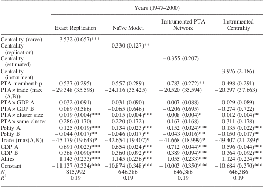
The results are presented in Table 3: Model 1 presents the results of the straight replication, whereas Models 2–4 present the naïve and the two corrected models, using the sample from our PTA instrument equation. The side-by-side comparison of results reveals several intriguing differences between the naïve model and the two IV approaches. The coefficient on centrality changes from 0.33 and statistically significant in the naïve model to statistically insignificant in the two models with corrections.
Endogeneity and Centrality Scores. Replication and Extension of Hafner-Burton & Montgomery (Reference Hafner-Burton and Montgomery2008)
Note: Exact replication re-estimates Hafner-Burton and Montgomery (Reference Hafner-Burton and Montgomery2008, Model 1 of Table 1), using the data provided by the authors. The differences in sample size between exact replication and other models are due to missingness on the variables used to construct the instruments. The correlation between the centrality variable in the naïve model and instrumented network model is 0.42, whereas that between the naïve model and instrumented Centrality model is 0.55. The exact and naïve models employ the same centrality variable.
PTA=preferential trade agreements; GDP=gross domestic product.
*p<0.05, **p<0.01, ***p<0.001.
The great variation in the estimated effect of centrality is somewhat surprising in light of the findings from our Monte Carlo analysis. There we saw little change in the estimates for centrality across approaches, though we did see some modest bias using the uncorrected centrality score in the direction of the correlation.
High error correlation or endogeneity, therefore, seems particularly likely to lead to a Type I error (erroneously finding statistical significance), when the direction of the error correlation (positive/negative) coincides with the hypothesized direction of the coefficient on the offending variable. Uncorrected, a positive error correlation makes a positive coefficients appear greater than it actually is, whereas a negative error correlation makes negative coefficients appear “more negative.” Both of the IV models, on the other hand, produce virtually unbiased estimates. Here the coefficients from the IV approaches are signed in opposite directions, but given that neither of them produces a significant finding perhaps we should not read too much into that. It seems, however, that the relationship between centrality and sanctions may need further exploration.
Conclusion
Although network analysis specifically challenges the assumption of independence among individual observations within the data set, in practice, many network approaches have not yet been fully adapted to the use with political science data. In the view of growing attention to network analysis within our discipline, surprisingly few studies have explored the interplay between the network tools and common political science data issues. In this paper, we highlight and propose a solution to one such issue—endogeneity between network measures, used as right-hand regressors, and the outcome variable.
Although the issue of endogeneity is relevant to a wide array of empirical relationships, it may become especially acute within the networks context, as endogeneity and the resulting bias in the estimates may be further exacerbated, owing to the nonlinear functional forms of many widely used network measures. As is the case with non-network approaches, possible endogeneity, however, can be addressed by implementing either of two relatively straightforward adaptations of an IV two-stage estimation approach. We support our argument with both Monte Carlo analyses and replications of several existing studies, which highlight the substantial empirical consequences of ignoring bias.
Our current results point toward a number of future investigations. First, there is a need for more research on the nature of the bias introduced by using raw or “uncorrected” network scores. Although our preliminary results suggest that there may not be a “one-size-fit-all” solution, and that various network-based or relational measures and scores might need to be studied individually, we believe that the use of network measures has become sufficiently ubiquitous to warrant such research. Second, as with any IV approach, the quality of our estimates depends directly upon the quality of the instrument. Exploring how variation in the ability of researchers to properly explain the relational variable should also be of interest. This will more generally lead to a root mean squared error comparison of the instrumented versus raw network measure. Third, an extension for discrete network connections would be worth exploring. There is also a need for alternate approaches for network measures that assume binary connections, in which case the continuously measured instrument used to calculate the measure might require weighting, such as that by the probability of a connection. Finally, it would be helpful to explore the consequences of endogeneity through additional Monte Carlo work. For instance, our results appear to show some bias for S scores, but that bias also appears to be small relative to the precision of the estimates, especially in comparison with the results for SEq scores. Whether this results from our particular setup or suggests a general greater robustness of S scores is worthy of further investigation.
Note that we limited our analysis to exploring only the effects of correlation between the error terms for each unit in the relational and outcome equations. Beyond that, we assume independent and identically distributed errors in the two equations. In practice, many situations may certainly not meet this assumption; once we introduce correlation between errors within equations, the effects of endogeneity could change dramatically, as the network score calculation could then include many elements correlated with the outcome of interest. Given the frequency of cross-sectional time-series applications of network scores, exploring the possible consequences of autocorrelation in the relational measures could also be worthwhile.
An obvious next step to account for these sorts of interdependencies would be to move to a network-based estimation approach for modeling either the first or second stage in our instrumented network approach. From a statistical point of view the consequences of endogeneity will tend to be the same; as noted above when we treated the second stage outcome as dichotomous, undirected ties and estimated the resulting network as an ERGM, we saw similar evidence of bias in the uncorrected approach, even when including common network measures such as density, reciprocity, and triads, but apparently unbiased estimates using our instrumented network approach. One could also consider extending this to utilize an ERGM for the relational variable. Still, in empirical applications, using an ERGM would potentially help produce better estimates by accounting for other forms of network interdependence. Latent space approaches could also work for either continuous or binary outcome variables (Hoff, Raftery and Handcock Reference Hoff, Raftery and Handcock2002; Hoff and Ward Reference Hoff and Ward2004). If the networks that connect units in the first and second stages share a similar structure, then ignoring them would help contribute to endogeneity by inducing high degrees of correlation between the error terms in the two equations. Even if this is not the case, applying either of IV approaches should help provide more appropriate measures of uncertainty, which matters as our re-sampling approach accounts for uncertainty in the first-stage estimates. As our use of ERGMs in our SEq replication shows, very different results can emerge compared with a simple logit (Hoff, Raftery and Handcock Reference Hoff, Raftery and Handcock2002; Hoff and Ward Reference Hoff and Ward2004).
Beyond the direct implications for network research, our results raise more general questions about the calculation of network-level measures in the presence of endogeneity. Besides those examined here, other examples include measures of network polarity, economic interdependence, or spatial-lag models. As the endogeneity varies across actors, bias in coefficients may be added or even multiplied in the process of calculation of such measures. At a minimum, our results call for a further investigation of the effects of endogeneity on these scores’ use as independent variables.
Acknowledgement
Previous versions of this paper have been presented at the 2012 European Political Science Association meeting in Berlin and the 2013 Spatial Models of Politics in Europe and Beyond at Texas A&M. We would like to thank all participants of these conferences who gave us feedback and suggestions. We would like to especially acknowledge Vera Troeger, Guy Whitten, Curt Signorino, Rob Franzese, Jude Hays, Havard Hegre, and the three anonymous reviewers.
Supplementary Material
To view supplementary material for this article, please visit http://dx.doi.org/10.1017/psrm.2015.34