Taylor–Couette–Poiseuille flow with a weakly permeable inner cylinder: absolute instabilities and selection of global modes

Nils Tilton; Denis Martinand

doi:10.1017/jfm.2018.437

Taylor–Couette–Poiseuille flow with a weakly permeable inner cylinder: absolute instabilities and selection of global modes

Published online by Cambridge University Press: 26 June 2018

Nils Tilton

and

Denis Martinand

Show author details

Nils Tilton: Affiliation:
Department of Mechanical Engineering, Colorado School of Mines, Golden, CO 80401, USA
Denis Martinand*: Affiliation:
Aix-Marseille Université, CNRS, Centrale Marseille, M2P2, 13013 Marseille, France
*: †Email address for correspondence: denis.martinand@univ-amu.fr

Article contents

Abstract
Introduction
Global modes in axially varying Taylor–Couette–Poiseuille flow
Global modes in direct numerical simulations
Discussion
Conclusions and outlook
References

Rights & Permissions

Abstract

Variations in the local stability of the flow in a Taylor–Couette cell can be imposed by adding an axial Poiseuille flow and a radial flow associated with one or both of the cylinders being permeable. At a given rotation rate of the inner cylinder, this results in adjacent regions of the flow that can be simultaneously stable, convectively unstable, and absolutely unstable, making this system fit for studying global modes of instability. To this end, building on the existing stability analysis in absolute modes developing over axially invariant base flows, we consider the case of axially varying base flows in systems for which the outer cylinder is impermeable, and the inner cylinder is a weakly permeable membrane through which the radial flow is governed by Darcy’s law. The frameworks of linear and nonlinear global modes are used to describe the instabilities and assess the results of direct numerical simulations using a dedicated pseudospectral method. Three different axially evolving set-ups are considered. In the first, fluid injection occurs along the full inner cylinder. In the second, fluid extraction occurs along the full inner cylinder. Besides its fundamental interest, this set-up is relevant to filtration devices. In the third, fluid flux through the inner cylinder evolves from extraction to injection as cross-flow reversal occurs. In agreement with the global mode analyses, the numerical simulations develop centrifugal instabilities above the predicted critical rotation rates and downstream of the predicted axial locations. The global mode analyses do not fully explain, however, that the instabilities observed in the numerical simulations take the form of axial stacks of wavepackets characterized by jumps of the temporal frequency.

JFM classification

Instability: Absolute/convective instability Instability: Nonlinear instability

Information

Type: JFM Papers
Information: Journal of Fluid Mechanics , Volume 849 , 25 August 2018, pp. 741 - 776
DOI: https://doi.org/10.1017/jfm.2018.437 [Opens in a new window]
Copyright: © 2018 Cambridge University Press

1 Introduction

Linear stability analysis has matured substantially since its first successful predictions of thermoconvective instabilities in Rayleigh–Bénard convection by Rayleigh (Reference Rayleigh1916) and centrifugal instabilities in Taylor–Couette flow by Taylor (Reference Taylor1923). Nevertheless, these two classical systems remain actively studied to advance our understanding of hydrodynamic instabilities and test new approaches of stability analysis (Koshmieder Reference Koshmieder1993, provides a thorough presentation). Though academic, Rayleigh–Bénard and Taylor–Couette flows bear sufficient resemblance to practical systems, and they can be readily studied experimentally to verify and motivate analytical approaches. The current work demonstrates that Taylor–Couette–Poiseuille (denoted TCP hereinafter) flow with a permeable inner cylinder provides a new opportunity to investigate how instabilities develop and tend to synchronize themselves in spatially varying open flows, a class of flows by which numerous industrial and geophysical systems are described. The current work, for example, is motivated by applications of supercritical TCP flow to membrane separation (Hallström & Lopez-Leiva Reference Hallström and Lopez-Leiva1978; Beaudoin & Jaffrin Reference Beaudoin and Jaffrin1989). More broadly, however, providing rigorous theoretical frameworks for synchronized, global, instabilities is pivotal to understand and predict how spatially varying open flows lose their stability and transition to turbulence. By comparing the results of theoretical analyses to the results of dedicated direct numerical simulations (DNS) of TCP flows, the current work shows that the dynamics of these global instabilities are still not fully understood beyond their critical conditions.

Early linear stability analyses of Taylor–Couette flow with a stationary outer cylinder considered the ideal case of infinitely extended concentric cylinders. Temporal stability analyses found standing wave instabilities that vary sinusoidally in the axial direction. Excellent agreement between experimental, numerical, and theoretical results are observed for the transition to supercritical flows, owing to the pitchfork nature of the bifurcation. The addition of a mean axial flow, producing TCP flow, can similarly be studied theoretically by considering infinitely extended cylinders between which instabilities vary sinusoidally in the axial direction. This shows that a Hopf bifurcation produces instability in the form of propagating waves. Mean axial flow also stabilizes the appearance of centrifugal instability in comparison to Taylor–Couette systems (see DiPrima Reference DiPrima1960; Donnelly & Fultz Reference Donnelly and Fultz1960; Chung & Astill Reference Chung and Astill1977; Johnson & Lueptow Reference Johnson and Lueptow1997, among many publications). For small mean axial velocity, instabilities appear as toroidal vortices travelling axially. With increasing mean axial velocity, these are superseded by travelling helical vortices. For sufficiently large axial flows, shear instabilities can also develop (Meseguer & Marques Reference Meseguer and Marques2002; Cotrell & Pearlstein Reference Cotrell and Pearlstein2004). The current work, however, will consider only centrifugal instabilities.

The addition of mean axial flow motivates two new approaches to modelling instabilities, due to the fact the system is now ‘open’. First, the mean flow-induced non-normality of the unstable modes can produce transient instabilities (see Chomaz Reference Chomaz2005, for a review). Second, considering the impulse response of the flow (the Green’s function) produces instabilities of finite axial extent. This motivates a distinction between convective and absolute instabilities (Huerre & Monkewitz Reference Huerre and Monkewitz1985, for instabilities in fluid flows). Convective instabilities grow in space and amplitude, but are advected downstream such that they eventually wash out of finite-length domains. In contrast, absolute instabilities grow sufficiently to overcome mean advection and invade an entire system, both up- and downstream. Convective/absolute stability analysis has been applied to Taylor vortices (Büchel et al. Reference Büchel, Lücke, Roth and Schmitz1996) and extended to helical vortices (Martinand, Serre & Lueptow Reference Martinand, Serre and Lueptow2009; Altmeyer, Hoffmann & Lücke Reference Altmeyer, Hoffmann and Lücke2011).

Most instabilities of practical interest develop on ‘imperfect’ base flows that vary spatially in more than one direction. In addition, end effects in open flows are more critical experimentally and numerically than in closed flows. In open flows, inlet conditions are advected by the mean flow and impact the whole domain, as observed by Babcock, Ahlers & Cannell (Reference Babcock, Ahlers and Cannell1991, Reference Babcock, Ahlers and Cannell1994) for TCP flows. Outlet conditions can also impact the instabilities developing within the system, as observed in rotating-disk flows (Pier Reference Pier2013; Appelquist et al. Reference Appelquist, Alfredsson, Schlatter and Lingwood2016). Therefore, experiments and numerical simulations often use specific inlet and outlet configurations that modify physical or geometrical characteristics along the mean flow direction to isolate instabilities developing in the core of the system. For example, experimental set-ups of Rayleigh–Bénard–Poiseuille convection often use a tailored ‘thermal entry’ where a temperature difference between the plates is slowly imposed to a developed Poiseuille flow (Nicolas Reference Nicolas2002). Therefore, introducing a degree of inhomogeneity in the base flow of the stability analysis, in the form of variations of its physical or geometrical characteristics, is relevant, if not required.

When considering the stability of an axially varying base flow with autonomous boundary conditions, instabilities take the form of synchronized modes called ‘global’ modes. A classical example is the von Kármán vortex street (Provansal, Mathis & Boyer Reference Provansal, Mathis and Boyer1987). The direction of the mean flow is then an extra eigendirection and such global modes can be computed numerically (see Theofilis Reference Theofilis2003, for a review). Computationally more affordable analyses of global modes are possible when the base flow varies slowly in the mean flow direction. Such base flows are often called ‘weakly non-parallel’. In this case, analyses can consider a convective/absolute stability analysis that approximates the local base flow as axially invariant, albeit with the physical and geometrical parameters set at the local values of the axially varying base flow. For flows that are everywhere stable or convectively unstable, perturbations can grow while in convectively unstable regions, but they either decay when reaching a stable region or they advect out of the system. Global instability arises when self-sustained localized perturbations occur in a region of local absolute instability. Analytical approaches to global modes consequently build on how absolute instabilities travel and saturate over axially varying base flows and look for a specific axial location that can act as a wavemaker and govern the global mode by imposing its critical conditions and frequency.

Two classes of wavemakers have emerged (see Huerre & Monkewitz Reference Huerre and Monkewitz1990; Huerre Reference Huerre, Batchelor, Moffatt and Worster2000; Chomaz Reference Chomaz2005, for reviews). The first, based on the linear dynamics of the absolute instability, locates the wavemaker where this absolute instability reaches its maximum local amplification. If the local amplification decreases monotonically in the axial direction, global modes can be obtained in a semi-infinite domain and the wavemaker will occur at the inlet (Monkewitz, Huerre & Chomaz Reference Monkewitz, Huerre and Chomaz1993). Conversely, the wavemaker will occur at the outlet if the local amplification increases monotonically (Healey Reference Healey2010). If the local amplification increases then decreases axially, the wavemaker will settle within the domain (Monkewitz et al. Reference Monkewitz, Huerre and Chomaz1993). Critical conditions and frequencies of global modes are computed from the linear dispersion relation for absolute instabilities. As the flow departs from criticality, the related nonlinear dispersion relation leads to the saturated state of the global mode, including a modification of its frequency (Pier & Huerre Reference Pier and Huerre1996; Couairon & Chomaz Reference Couairon and Chomaz1997; Chomaz & Couairon Reference Chomaz and Couairon1999; Pier, Huerre & Chomaz Reference Pier, Huerre and Chomaz2001).

The second class of wavemakers is based on the nonlinear counterpart of an absolute instability. It considers the behaviour of the front formed in the amplitude of the instability at the boundary between the upstream region of unperturbed base flow and the downstream region of saturated instability. Following Dee & Langer (Reference Dee and Langer1983), this front can be ‘pulled’ by the unperturbed flow and propagate upstream until it reaches the boundary between the convectively and absolutely unstable regions where it gets pinned and acts as a wavemaker. As these dynamics are governed by the unperturbed flow, the critical conditions and frequencies of global modes are computed from the linear dispersion relation for absolute instabilities (Pier et al. Reference Pier, Huerre, Chomaz and Couairon1998, Reference Pier, Huerre and Chomaz2001). According to van Saarloos & Hohenberg (Reference van Saarloos and Hohenberg1992), the front could also be ‘pushed’ by the saturated instability. The present study implements three selection mechanisms introduced by Monkewitz et al. (Reference Monkewitz, Huerre and Chomaz1993), Pier et al. (Reference Pier, Huerre, Chomaz and Couairon1998) and Healey (Reference Healey2010). These rely exclusively on the linear local dispersion relation to determine the location of the wavemaker, and the critical condition and frequency of the global mode.

The theoretical approaches above were initially developed in the literature for model scalar equations, including the one-dimensional complex Ginzburg–Landau equation or the two-dimensional vorticity equation for shear flows. Our work fits within a series of works extending these approaches to the three-dimensional Navier–Stokes equations in combination with DNS or experiments in configurations such as rotating disks (Pier Reference Pier2003; Appelquist et al. Reference Appelquist, Schlatter, Alfredsson and Lingwood2015, Reference Appelquist, Alfredsson, Schlatter and Lingwood2016). Global modes in Rayleigh–Bénard–Poiseuille flow have received theoretical (Carrière & Monkewitz Reference Carrière and Monkewitz2001), numerical (Martinand, Carrière & Monkewitz Reference Martinand, Carrière and Monkewitz2006) and experimental (Grandjean & Monkewitz Reference Grandjean and Monkewitz2009) attention, with excellent agreement. For that case, the thermoconvective instability can be spatially altered by modifying the local temperature between the plates. Global modes in TCP flows are less studied because it is more difficult to spatially vary the centrifugal instabilities. Consider the case of a fixed outer cylinder of radius $r_{2}$ and a rotating inner cylinder with radius $r_{1}$ and angular velocity $\unicode[STIX]{x1D6FA}$ . Experimentally, the angular velocity cannot be smoothly varied along the axial direction. Consequently, the local stability must be altered indirectly.

The stability of TCP flow is governed by three control parameters. The first is the Taylor number $\mathit{Ta}=\unicode[STIX]{x1D6FA}r_{1}d/\unicode[STIX]{x1D708}$ (or rotating Reynolds number), where $\unicode[STIX]{x1D708}$ is the kinematic viscosity of the fluid and $d=r_{2}-r_{1}$ the gap width. The second is the radius ratio $\unicode[STIX]{x1D702}=r_{1}/r_{2}$ . The third is the axial Reynolds number $\unicode[STIX]{x1D6FD}=\overline{W}d/\unicode[STIX]{x1D708}$ , where $\overline{W}$ is the mean axial velocity. One method of locally increasing the instability of the TCP flow is to locally increase $r_{2}$ . This increases the gap width and the Taylor number $\mathit{Ta}$ , while decreasing the radius ratio $\unicode[STIX]{x1D702}$ and axial Reynolds number $\unicode[STIX]{x1D6FD}$ owing to the conservation of the axial mass flow rate. In § 5, we show that these changes can indeed promote centrifugal absolute instabilities. This approach is nevertheless impractical, as it requires a set of different outer cylinders that cannot be tuned easily. Though Taylor–Couette systems with varying radii have been studied experimentally and numerically in the absence of mean axial flow (Soward & Jones Reference Soward and Jones1983), no results with mean axial flow are available in the literature, to our knowledge.

The current study shows that the local stability of the TCP flow can be altered in a more controlled fashion by replacing one or both of the impermeable cylinders with permeable cylindrical membranes. As fluid exits or enters the annular region through these membranes, the mean axial flow increases or decreases and thus alters the local stability. This configuration for TCP flow is used in an application called rotating filtration, in which a cylindrical semi-permeable membrane rotates within a concentric fixed impermeable cylinder. As suspension is introduced at one end of the annulus, fluid is extracted through the inner cylinder, and concentrate exits the opposite end of the annulus (see Lee & Lueptow Reference Lee and Lueptow2004, and references therein for applications). This approach reduces the accumulation of contaminants on the membrane surface because the centrifugal instabilities wash them away from the membrane (Schwille, Mitra & Lueptow Reference Schwille, Mitra and Lueptow2002). Due to the small permeability of the membrane, the base flow in rotating filtration systems varies slowly in the axial direction, thus opening the door to a global mode analysis.

Previous analytical and numerical studies have considered the related case of TCP flow with uniform radial through-flows applied at the inner and outer cylinders. The radial flows are applied such that the mass flux entering one cylinder equals that exiting the other cylinder. The resulting base flow is axially invariant and amenable to convective/absolute stability analysis (see Martinand et al. Reference Martinand, Serre and Lueptow2009, and references therein). Until recently, stability analysis of global modes in rotating filtration has been hindered by analytical and numerical difficulties related to the fact that the filtrate flow through the membrane is driven by the transmembrane pressure difference. Considering the base flow, this leads to a simultaneous coupling between the axial pressure drop and the transmembrane pressure. A generalized analytical solution, sketched in figure 1, has been found, however (Tilton et al. Reference Tilton, Martinand, Serre and Lueptow2010), as an asymptotic expansion that couples the transmembrane flow and pressure using Darcy’s law. Centrifugal instabilities in rotating filtration systems are also challenging to simulate numerically because the membrane introduces an additional coupling between the velocity and the pressure on the permeable cylinder. As a result, traditional pressure solvers for integrating the Navier–Stokes and continuity equations in time can fail. Tilton et al. (Reference Tilton, Serre, Martinand and Lueptow2014) have addressed this issue by developing an efficient, non-iterative, projection method tailored to simulating membranes in unsteady three-dimensional fluid flows.

Figure 1.

(a) Radial and axial velocities of the laminar base flow for the axially varying problem in a meridional plane. The outer cylinder is impermeable while fluid flows across the inner permeable cylinder, according to Darcy’s law, leading to a base flow varying along the axial direction. Panel (b) shows the azimuthal velocity of the base flow in an equatorial plane.

The current study is organized as follows. In § 2, we present the geometry, governing equations, base state and global mode analyses. In § 3, we compare the predictions of our global mode analyses with dedicated DNS. In § 4, we further address the frequency jumps, a specific feature observed in the DNS, and test the robustness of these instabilities by applying more intrusive inlet conditions or higher Taylor numbers to the DNS. After summarizing our results, their implications for rotating filtration and possible future work are then discussed in § 5.

2 Global modes in axially varying Taylor–Couette–Poiseuille flow

Hereinafter, we use cylindrical coordinates $(r,\unicode[STIX]{x1D703},z)$ , in which the velocity vector is denoted $\boldsymbol{V}=(U,V,W)^{t}$ . As sketched in figure 1, we consider an open Taylor–Couette cell with a stationary outer cylinder of radius $r_{2}$ and an inner rotating cylinder of radius $r_{1}$ . The outer cylinder is impermeable, while the inner cylinder is made of a thin permeable membrane that is shaded grey in figure 1. The rotating membrane surrounds a cylindrical cavity that is maintained at a constant pressure $P_{ref}$ . The radial fluid velocity $U(r_{1},\unicode[STIX]{x1D703},z)$ through the permeable membrane depends on the transmembrane pressure difference, as described by Darcy’s law:

(2.1)

$$\begin{eqnarray}U(r_{1},\unicode[STIX]{x1D703},z)=-\frac{\unicode[STIX]{x1D705}}{\unicode[STIX]{x1D707}h}[P(r_{1},\unicode[STIX]{x1D703},z)-P_{ref}],\end{eqnarray}$$

where $\unicode[STIX]{x1D705}$ is the membrane permeability (units $\text{m}^{2}$ ), $h$ is the membrane thickness and $\unicode[STIX]{x1D707}$ is the fluid dynamic viscosity. Note that the transmembrane flow in rotating filtration is typically quite small, such that it flows along a thin film on the inner rotating membrane. The assumption of constant $P_{ref}$ is consequently well justified, and without loss of generality, we set $P_{ref}=0$ .

Fluid flow in the annular region is governed by the incompressible Navier–Stokes and continuity equations. We non-dimensionalize these equations with respect to the gap width $d=r_{2}-r_{1}$ , characteristic time $d^{2}/\unicode[STIX]{x1D707}$ , characteristic pressure $\unicode[STIX]{x1D70C}\unicode[STIX]{x1D708}^{2}/d^{2}$ , and characteristic velocity $\unicode[STIX]{x1D708}/d$ , with $\unicode[STIX]{x1D70C}$ the density of the fluid. The flow is characterized by a Taylor number $\mathit{Ta}$ , radius ratio $\unicode[STIX]{x1D702}$ and non-dimensional permeability $\unicode[STIX]{x1D70E}$ :

(2.2a-c )

$$\begin{eqnarray}\mathit{Ta}=\frac{\unicode[STIX]{x1D6FA}r_{1}d}{\unicode[STIX]{x1D708}},\quad \unicode[STIX]{x1D702}=\frac{r_{1}}{r_{2}},\quad \unicode[STIX]{x1D70E}=\frac{\unicode[STIX]{x1D705}}{hd}.\end{eqnarray}$$

Hereinafter, all expressions are non-dimensional, unless otherwise stated. The governing Navier–Stokes and continuity equations then take the form:

(2.3a,b )

$$\begin{eqnarray}\displaystyle \frac{\unicode[STIX]{x2202}\boldsymbol{V}}{\unicode[STIX]{x2202}t}+\boldsymbol{V}\boldsymbol{\cdot }\unicode[STIX]{x1D735}\boldsymbol{V}=-\unicode[STIX]{x1D735}P+\unicode[STIX]{x1D6FB}^{2}\boldsymbol{V}\quad \text{and}\quad \unicode[STIX]{x1D735}\boldsymbol{\cdot }\boldsymbol{V}=0.\end{eqnarray}$$

On the outer cylinder, no-slip conditions are applied. On the permeable inner cylinder, the azimuthal and axial components of the velocity also satisfy the no-slip condition, while $U$ is related to the transmembrane pressure difference through Darcy’s law:

(2.4)

$$\begin{eqnarray}\left.\begin{array}{@{}c@{}}U(r_{1},\unicode[STIX]{x1D703},z)=-\unicode[STIX]{x1D70E}P(r_{1},\unicode[STIX]{x1D703},z)\quad \text{and}\quad U(r_{2},\unicode[STIX]{x1D703},z)=0\\ V(r_{1},\unicode[STIX]{x1D703},z)=\mathit{Ta}\quad \text{and}\quad V(r_{2},\unicode[STIX]{x1D703},z)=0\\ W(r_{1},\unicode[STIX]{x1D703},z)=W(r_{2},\unicode[STIX]{x1D703},z)=0.\end{array}\right\}\end{eqnarray}$$

The no-slip condition on the inner cylinder is guided by practical applications to membrane filtration, which use strongly anisotropic membranes with negligible slip. Focusing on the filtration of solutions, the dimensional ratio $\unicode[STIX]{x1D705}/h$ of membranes used in filtration units typically ranges from $10^{-10}$ m for reverse osmosis to $10^{-4}$ m for microfiltration. Though the gap $d$ might vary substantially with the size of the unit, the non-dimensional permeability $\unicode[STIX]{x1D70E}$ is thus a very small quantity in real systems.

2.1 Base flow

The transmembrane pressure difference between the annulus and cavity drives a radial extraction or injection of fluid through the permeable cylinder. This in turn drives radial and axial flows that vary axially in the annular region. An analytical solution for the axially varying steady axisymmetric base flow $\boldsymbol{V}_{b}(r,z)$ has been found by Tilton et al. (Reference Tilton, Martinand, Serre and Lueptow2010) in the form of an asymptotic expansion about the small parameter $\unicode[STIX]{x1D700}=\sqrt{\unicode[STIX]{x1D70E}}$ , see appendix A. This base flow is a slowly varying function of the axial $z$ -coordinate, or equivalently, a function of a slow variable $\unicode[STIX]{x1D700}z$ . Based on this solution, a local axial Reynolds number is introduced:

(2.5)

$$\begin{eqnarray}\displaystyle \unicode[STIX]{x1D6FD}(z) & = & \displaystyle \overline{W}(z)=\frac{1}{\unicode[STIX]{x03C0}(r_{2}^{2}-r_{1}^{2})}\int _{r=r_{1}}^{r_{2}}\int _{\unicode[STIX]{x1D703}=0}^{2\unicode[STIX]{x03C0}}W_{b}(r,z)r\,\text{d}\unicode[STIX]{x1D703}\,\text{d}r\nonumber\\ \displaystyle & = & \displaystyle A_{1}\exp (z\sqrt{\unicode[STIX]{x1D701}\unicode[STIX]{x1D70E}})+A_{2}\exp (-z\sqrt{\unicode[STIX]{x1D701}\unicode[STIX]{x1D70E}}),\end{eqnarray}$$

with $W_{b}(r,z)$ as in appendix A and the geometrical factor

(2.6)

$$\begin{eqnarray}\unicode[STIX]{x1D701}=\frac{16\log \unicode[STIX]{x1D702}}{(r_{2}^{4}-r_{1}^{4})\log \unicode[STIX]{x1D702}+(r_{2}^{2}-r_{1}^{2})^{2}}.\end{eqnarray}$$

Constants $A_{1}$ and $A_{2}$ in (2.5) are first order in $\unicode[STIX]{x1D700}$ . They can be set by prescribing the axial Reynolds number $\unicode[STIX]{x1D6FD}(z)$ at two arbitrary locations $z=0$ and $z=L$ .

To characterize the transmembrane flow, we introduce a local radial Reynolds number, related to the axial one $\unicode[STIX]{x1D6FD}(z)$ by the conservation of mass:

(2.7)

$$\begin{eqnarray}\displaystyle \unicode[STIX]{x1D6FC}_{1}(z) & = & \displaystyle r_{1}U_{b}(r_{1},z)=\frac{r_{2}^{2}-r_{1}^{2}}{2}\frac{\text{d}\unicode[STIX]{x1D6FD}(z)}{\text{d}z}\nonumber\\ \displaystyle & = & \displaystyle \frac{\sqrt{\unicode[STIX]{x1D701}\unicode[STIX]{x1D70E}}(r_{2}^{2}-r_{1}^{2})}{2}[A_{1}\exp (z\sqrt{\unicode[STIX]{x1D701}\unicode[STIX]{x1D70E}})-A_{2}\exp (-z\sqrt{\unicode[STIX]{x1D701}\unicode[STIX]{x1D70E}})].\end{eqnarray}$$

This radial Reynolds number is second order in $\unicode[STIX]{x1D700}$ and, consequently, small. Owing to the exponential terms in (2.5) and (2.7), $\unicode[STIX]{x1D6FD}(z)$ and $\unicode[STIX]{x1D6FC}_{1}(z)$ only make sense over a finite axial length, assuming end effects can be ignored.

Figure 2.

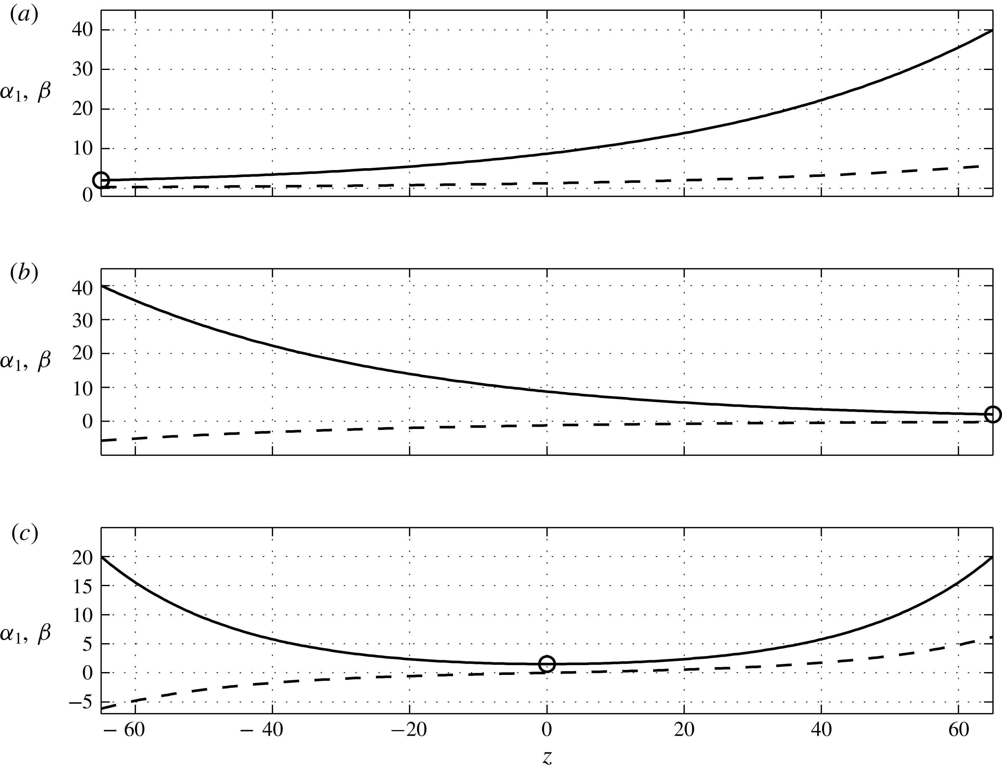
Three possible base flow variations of the axial Reynolds number $\unicode[STIX]{x1D6FD}(z)$ (solid lines) and radial Reynolds number $\unicode[STIX]{x1D6FC}_{1}(z)$ (dashed lines). (a) Results obtained when $\unicode[STIX]{x1D6FD}_{inlet}=2$ , $\unicode[STIX]{x1D6FD}_{outlet}=40$ and $\unicode[STIX]{x1D70E}=5\times 10^{-5}$ . The axial base flow $\unicode[STIX]{x1D6FD}(z)$ increases monotonically as fluid is injected along the membrane. The circle at the inlet marks the most unstable simple turning point as defined in § 2.2. (b) Results obtained when $\unicode[STIX]{x1D6FD}_{inlet}=40$ , $\unicode[STIX]{x1D6FD}_{outlet}=2$ and $\unicode[STIX]{x1D70E}=5\times 10^{-5}$ . The axial base flow $\unicode[STIX]{x1D6FD}(z)$ decreases monotonically as fluid is extracted along the membrane. The circle at the outlet marks the most unstable simple turning point as defined in § 2.2. (c) Results obtained when $\unicode[STIX]{x1D6FD}_{inlet}=20$ , $\unicode[STIX]{x1D6FD}_{outlet}=20$ and $\unicode[STIX]{x1D70E}=2.3\times 10^{-4}$ . The base flow $\unicode[STIX]{x1D6FD}(z)$ undergoes cross-flow reversal as $\unicode[STIX]{x1D6FC}_{1}(z)$ transitions from extraction to injection at $z=0$ . The circle at the centre marks the most unstable double turning point as defined in § 2.2.

The constants $A_{1}$ and $A_{2}$ in (2.5) and (2.7) are selected so as to consider three different types of base flows over a finite axial length, as shown in figure 2. Panels (a–c) all show an increase along the axial direction of the radial Reynolds number on the inner cylinder $\unicode[STIX]{x1D6FC}_{1}(z)$ (dashed line). This occurs due to the axial pressure drop driving the mean axial flow. Figure 2(a) demonstrates an ‘injection’ configuration in which the axial Reynolds number $\unicode[STIX]{x1D6FD}(z)$ (solid line) increases monotonically with $z$ because fluid is entering the annulus from the membrane along the entire axial length $L$ of the domain. Figure 2(b) demonstrates an ‘extraction’ configuration in which $\unicode[STIX]{x1D6FD}(z)$ decreases monotonically with $z$ due to the fact that fluid is leaving the annulus through the membrane along the entire axial length. Finally, figure 2(c) shows ‘cross-flow reversal’ in which the transmembrane flow transitions from extraction to injection.

2.2 Global modes and their selection mechanisms

We now proceed to analytically address the centrifugal instabilities as global modes. The velocity and pressure fields are decomposed as $[\boldsymbol{V},P]=[\boldsymbol{V}_{b},P_{b}]+[\boldsymbol{V}_{p},P_{p}]$ , where $[\boldsymbol{V}_{b}(r,z),P_{b}(r,z)]$ is the base flow presented in § 2.1 and appendix A, and $[\boldsymbol{V}_{p}(r,\unicode[STIX]{x1D703},z,t),P_{p}(r,\unicode[STIX]{x1D703},z,t)]$ is a small time-dependent perturbation. Linearizing the problem (2.3)–(2.4) about the base flow $[\boldsymbol{V}_{b},P_{b}]$ produces an autonomous system of partial differential equations admitting synchronized solutions, i.e. solutions presenting a common, complex, temporal frequency $\unicode[STIX]{x1D714}^{glob}$ such that $[\boldsymbol{V}_{p},P_{p}]=[\boldsymbol{V}_{p}^{glob}(r,\unicode[STIX]{x1D703},z),P_{p}^{glob}(r,\unicode[STIX]{x1D703},z)]\exp (-\text{i}\unicode[STIX]{x1D714}^{glob}t)$ . Though the spatial shape functions $[\boldsymbol{V}_{p}^{glob},P_{p}^{glob}]$ can be obtained by solving a multi-dimensional eigenproblem numerically, we leverage the slow axial variation of $\boldsymbol{V}_{b}$ to reduce the numerical cost to a one-dimensional eigenproblem. Based on the weak $z$ -dependence of $\boldsymbol{V}_{b}(r,z)$ , the instabilities are expressed in the form of the Wentzel–Kramers–Brillouin (WKB) ansatz of a wavepacket:

(2.8)

$$\begin{eqnarray}[\boldsymbol{V}_{p},P_{p}]=[\boldsymbol{v}_{p}^{glob}(r,z),p_{p}^{glob}(r,z)]\exp (\text{i}\unicode[STIX]{x1D713})\quad \text{with}~\unicode[STIX]{x1D713}=\int _{z_{0}}^{z}k(z^{\prime })\,\text{d}z^{\prime }+n\unicode[STIX]{x1D703}-\unicode[STIX]{x1D714}^{glob}t.\end{eqnarray}$$

With this framework, the shape functions $[\boldsymbol{v}_{p}^{glob}(r,z),p_{p}^{glob}(r,z)]$ and the local axial wavenumber $k(z)$ are slowly varying functions of $z$ or, equivalently, functions of the slow variable $\unicode[STIX]{x1D700}z$ . Injecting ansatz (2.8) into (2.3)–(2.4) linearized about the base flow $[\boldsymbol{V}_{b},P_{b}]$ leads one to expand $\unicode[STIX]{x1D714}^{glob}$ and $[\boldsymbol{v}_{p}^{glob},p_{p}^{glob}]$ in powers of $\unicode[STIX]{x1D700}$ and solve a hierarchy of systems of ordinary differential equations.

The leading order ( $\unicode[STIX]{x1D700}^{0}$ ) of the WKB expansion satisfies a local generalized eigenvalue problem

(2.9)

$$\begin{eqnarray}\unicode[STIX]{x1D63C}(k(z),n,\boldsymbol{V}_{b,0}(r,z))[\boldsymbol{v}_{p}^{loc},p_{p}^{loc}]=\unicode[STIX]{x1D714}^{loc}\unicode[STIX]{x1D63D}[\boldsymbol{v}_{p}^{loc},p_{p}^{loc}],\end{eqnarray}$$

where the superscripts on eigenvector $[\boldsymbol{v}_{p}^{loc},p_{p}^{loc}]$ and eigenvalue $\unicode[STIX]{x1D714}^{loc}$ stress that (2.9) depends on the local base flow as discussed below. The operator $\unicode[STIX]{x1D63C}$ is a $r$ -differential operator, parametrized by the axial coordinate $z$ through the wavenumber $k(z)$ and the base flow $\boldsymbol{V}_{b,0}(r,z)$ , the leading order $\unicode[STIX]{x1D700}^{0}$ of the base flow $\boldsymbol{V}_{b}(r,z)$ . To include axial variations at order $\unicode[STIX]{x1D700}^{0}$ , the base flow reported in appendix A must be slightly modified, so that the axial Reynolds number $\unicode[STIX]{x1D6FD}(z)$ , given by (2.5), is considered as order $\unicode[STIX]{x1D700}^{0}$ instead of $\unicode[STIX]{x1D700}^{1}$ . Referring to the expressions in appendix A, this produces a leading-order base flow that is identical to axially invariant TCP flow, composed of the axial velocity $W_{b}=\unicode[STIX]{x1D6FD}(z)w_{b}(r)$ , and the leading order of the azimuthal velocity, $\mathit{Ta}v_{b,0}(r)$ . Consequently, problem (2.9) amounts to the stability of axially invariant TCP flow with the parameter $\unicode[STIX]{x1D6FD}$ set to $\unicode[STIX]{x1D6FD}(z)$ .

As the convective/absolute stability of this flow is well studied (Recktenwald, Lücke & Müller Reference Recktenwald, Lücke and Müller1993; Martinand et al. Reference Martinand, Serre and Lueptow2009; Altmeyer et al. Reference Altmeyer, Hoffmann and Lücke2011), it is only summarized in appendix B and results relevant for the global mode analysis in § 3 briefly presented. Figure 3 shows the results, in the form of the critical Taylor numbers and critical frequencies, of the local convective/absolute stability problem (B 2), as a function of $\unicode[STIX]{x1D6FD}$ , for $\unicode[STIX]{x1D702}$ set to 0.85. Beyond their respective critical conditions, figure 3 also sheds light on some differences and similarities between convective and absolute instabilities. Whereas absolute critical modes are always travelling toroidal vortices ( $n_{crit}^{abs}=0$ ), convective critical modes become helical vortices for axial Reynolds numbers above $\unicode[STIX]{x1D6FD}=13.8$ . The critical frequency is a growing function of the axial Reynolds number $\unicode[STIX]{x1D6FD}$ for both convective and absolute instabilities. For axisymmetric vortices, absolute and convective instabilities exhibit very similar frequencies. It is therefore difficult to discriminate between convective and absolute toroidal instabilities on the basis of their temporal frequencies.

Figure 3.

Local linear stability results for the critical convective (solid curves) and absolute (dashed curves) modes of instability, as functions of the axial Reynolds number $\unicode[STIX]{x1D6FD}$ , for radius ratio $\unicode[STIX]{x1D702}=0.85$ . (a) Critical Taylor numbers $\mathit{Ta}_{crit}^{conv}$ and $\mathit{Ta}_{crit}^{abs}$ . (b) Critical frequencies $\unicode[STIX]{x1D714}_{crit}^{conv}$ and $\unicode[STIX]{x1D714}_{crit}^{abs}$ . Digits in (a) indicate the azimuthal wavenumbers of the critical convective modes $n_{crit}^{conv}$ .

As the local stability problem (2.9) is parametrized by the axial coordinate $z$ , its solution provides no selection criterion for a global mode frequency $\unicode[STIX]{x1D714}^{glob}$ per se. A selection criterion is usually related to specific axial location(s) from which the wavepacket can propagate both down- and upstream, i.e. to a ‘turning point’ $z_{t.p.}$ where the group velocity vanishes:

(2.10)

$$\begin{eqnarray}\frac{\unicode[STIX]{x2202}\unicode[STIX]{x1D714}}{\unicode[STIX]{x2202}k}(z_{t.p.})=0.\end{eqnarray}$$

Hereinafter, the $(z_{t.p.})$ -dependence means that the group velocity is computed from the resolution of the local stability problem (B 2) where the $\unicode[STIX]{x1D6FD}$ is set to $\unicode[STIX]{x1D6FD}(z_{t.p.})$ . Condition (2.10) can be satisfied by an absolute mode that is unstable if the system is locally above the critical conditions for absolute instabilities. A turning point then acts as a wavemaker if it imposes the temporal frequency of the local absolute mode, i.e. $\unicode[STIX]{x1D714}^{abs}(z_{t.p.})$ to the rest of the domain. Critical conditions for the global mode, $\mathit{Ta}_{crit}^{glob}$ , can be then deduced from the growth rate of the absolute mode at the turning point, i.e. the imaginary part of $\unicode[STIX]{x1D714}^{abs}(z_{t.p.})$ .

Several analytical selection criteria for identifying wavemakers are available in the literature. They begin by identifying the axial location of a turning point. We implement two linear selection criteria introduced in Monkewitz et al. (Reference Monkewitz, Huerre and Chomaz1993) and extended in Healey (Reference Healey2010). Both criteria consider a turning point located where the flow is locally the most unstable, i.e. where $\text{Im}(\unicode[STIX]{x1D714}^{abs}(z))$ is maximum. Elaborating on figure 3(a), the growth rate of the critical absolute instabilities is a decreasing function of the axial Reynolds number $\unicode[STIX]{x1D6FD}$ : $\unicode[STIX]{x2202}_{\unicode[STIX]{x1D6FD}}\text{Im}(\unicode[STIX]{x1D714}_{crit}^{abs})=-\unicode[STIX]{x2202}_{\mathit{Ta}}\text{Im}(\unicode[STIX]{x1D714}_{crit}^{abs})/\unicode[STIX]{x2202}_{\mathit{Ta}}\unicode[STIX]{x1D6FD}_{crit}^{abs}<0$ . A local maximum of the growth rate $\text{Im}(\unicode[STIX]{x1D714}^{abs}(z))$ therefore corresponds to a local minimum of $\unicode[STIX]{x1D6FD}(z)$ .

The first selection criterion (Monkewitz et al. Reference Monkewitz, Huerre and Chomaz1993) addresses cases where an island of absolute instability is surrounded by a sea of stability, up- and downstream. Though this criterion assumes an infinite axial domain, it also applies to finite axial configurations in which the inlet is locally stable and the outlet is either locally stable or convectively unstable. The axial flow shown in figure 2(c) presents a minimum of $\unicode[STIX]{x1D6FD}(z)$ located within the fluid domain, constituting a potentially unstable ‘double turning point’. The second selection criterion addresses cases of semi-infinite axial extent that present a maximum absolute instability at the inlet or outlet, as in Monkewitz et al. (Reference Monkewitz, Huerre and Chomaz1993) and Healey (Reference Healey2010), respectively. Though this criterion assumes a semi-infinite axial extent, it also applies for systems of finite axial extent in which the outlet or the inlet are locally stable or convectively unstable. Figure 2 demonstrates base flows that present minimums of $\unicode[STIX]{x1D6FD}(z)$ at the inlet (panel a) or the outlet (panel b). These constitute potentially unstable ‘single turning points’. A linear selection criterion therefore leads to critical conditions in term of a critical Taylor number $\mathit{Ta}_{crit}^{glob}$ , together with characteristics of the global mode at these critical conditions, such as the critical frequency $\unicode[STIX]{x1D714}_{crit}^{glob}$ .

2.2.1 Linear selection by a double turning point

Based on the local stability problem at a double turning point $z_{d.t.p.}$ , where the flow is locally the most unstable, the local growth rate also satisfies:

(2.11a,b )

$$\begin{eqnarray}\frac{\unicode[STIX]{x2202}\text{Im}(\unicode[STIX]{x1D714}^{abs})}{\unicode[STIX]{x2202}z}(z_{d.t.p.})=0\quad \text{and}\quad \frac{\unicode[STIX]{x2202}^{2}\text{Im}(\unicode[STIX]{x1D714}^{abs})}{\unicode[STIX]{x2202}z^{2}}(z_{d.t.p.})<0,\end{eqnarray}$$

in addition to condition (2.10). As the $z$ -dependence of the dispersion relation amounts to the axial variations of the axial Reynolds number $\unicode[STIX]{x1D6FD}$ , condition (2.11) requires:

(2.12a,b )

$$\begin{eqnarray}\frac{\text{d}\unicode[STIX]{x1D6FD}}{\text{d}z}(z_{d.t.p.})=0\quad \text{and}\quad \frac{\text{d}^{2}\unicode[STIX]{x1D6FD}}{\text{d}z^{2}}(z_{d.t.p.})>0.\end{eqnarray}$$

This condition is achieved in the case of cross-flow reversal, as illustrated in figure 2(c), where $z_{d.t.p.}$ is indicated by a circle.

At leading order, the global mode frequency imposed by a double turning point is $\unicode[STIX]{x1D714}^{loc}=\unicode[STIX]{x1D714}^{abs}(z_{d.t.p.})$ , computed by solving the local stability problem (B 2) for the most unstable absolute instability, with $\unicode[STIX]{x1D6FD}$ set to $\unicode[STIX]{x1D6FD}(z_{d.t.p.})$ . A global mode governed by a double turning point should thus be observed as the Taylor number overcomes the critical absolute Taylor number at the double turning point:

(2.13)

$$\begin{eqnarray}\mathit{Ta}_{crit}^{loc}=\mathit{Ta}_{crit}^{abs}(z_{d.t.p.}).\end{eqnarray}$$

The global mode is characterized by the real frequency:

(2.14)

$$\begin{eqnarray}\unicode[STIX]{x1D714}_{crit}^{loc}=\unicode[STIX]{x1D714}_{crit}^{abs}(z_{d.t.p.}).\end{eqnarray}$$

Following (4.21a) in Monkewitz et al. (Reference Monkewitz, Huerre and Chomaz1993), matching the perturbation around this double turning point to the perturbation in the rest of the domain mathematically imposes a small correction to the frequency in the form:

(2.15)

$$\begin{eqnarray}\displaystyle \unicode[STIX]{x1D714}^{glob} & = & \displaystyle \unicode[STIX]{x1D714}^{loc}+\text{i}\frac{1}{2}\left.\frac{\unicode[STIX]{x2202}^{2}\unicode[STIX]{x1D714}}{\unicode[STIX]{x2202}k\unicode[STIX]{x2202}z}\right|^{abs}\pm \frac{1}{2}\left(\left.\frac{\unicode[STIX]{x2202}^{2}\unicode[STIX]{x1D714}}{\unicode[STIX]{x2202}k^{2}}\right|^{abs}\left.\frac{\unicode[STIX]{x2202}^{2}\unicode[STIX]{x1D714}}{\unicode[STIX]{x2202}z^{2}}\right|^{abs}-\left(\left.\frac{\unicode[STIX]{x2202}^{2}\unicode[STIX]{x1D714}}{\unicode[STIX]{x2202}k\unicode[STIX]{x2202}z}\right|^{abs}\right)^{2}\right)^{1/2}\nonumber\\ \displaystyle & = & \displaystyle \unicode[STIX]{x1D714}^{loc}\pm \frac{1}{2}\frac{\text{d}^{2}\unicode[STIX]{x1D6FD}}{\text{d}z^{2}}^{1/2}\left(\left.\frac{\unicode[STIX]{x2202}^{2}\unicode[STIX]{x1D714}}{\unicode[STIX]{x2202}k^{2}}\right|^{abs}\left.\frac{\unicode[STIX]{x2202}\unicode[STIX]{x1D714}}{\unicode[STIX]{x2202}\unicode[STIX]{x1D6FD}}\right|^{abs}\right)^{1/2}.\end{eqnarray}$$

Though the $(z_{d.t.p.})$ -dependences are dropped for convenience in (2.15), all quantities inferred from the local stability problem and $\unicode[STIX]{x1D6FD}(z)$ are computed at $z_{d.t.p.}$ . Equation (4.21a) in Monkewitz et al. (Reference Monkewitz, Huerre and Chomaz1993) also includes a term due to the corrections to the base flow at order $\unicode[STIX]{x1D700}^{1}$ . This term involves here the radial velocity $U_{b}=\text{d}\unicode[STIX]{x1D6FD}/\text{d}zu_{b}(r)$ and the correction to the azimuthal velocity $\text{d}\unicode[STIX]{x1D6FD}/\text{d}zv_{b,1}(r)$ . These components being proportional to $\text{d}\unicode[STIX]{x1D6FD}/\text{d}z$ , they vanish at the double turning point. The frequency correction in (2.15) is complex, and the sign in the expression is chosen so that $\text{Im}(\unicode[STIX]{x1D714}^{glob})<\text{Im}(\unicode[STIX]{x1D714}^{loc})$ , i.e. so that this correction is stabilizing. This stabilizing effect increases the critical Taylor number above which such a global mode can be observed, compared to the leading-order critical value (2.13):

(2.16)

$$\begin{eqnarray}\mathit{Ta}_{crit}^{glob}=\mathit{Ta}_{crit}^{loc}-\frac{1}{2}\frac{\text{d}^{2}\unicode[STIX]{x1D6FD}}{\text{d}z^{2}}^{1/2}\frac{\displaystyle \text{Im}\left(\pm \left(\left.\frac{\unicode[STIX]{x2202}^{2}\unicode[STIX]{x1D714}}{\unicode[STIX]{x2202}k^{2}}\right|_{crit}^{abs}\left.\frac{\unicode[STIX]{x2202}\unicode[STIX]{x1D714}}{\unicode[STIX]{x2202}\unicode[STIX]{x1D6FD}}\right|_{crit}^{abs}\right)^{1/2}\right)}{\displaystyle \text{Im}\left(\left.\frac{\unicode[STIX]{x2202}\unicode[STIX]{x1D714}}{\unicode[STIX]{x2202}\mathit{Ta}}\right|_{crit}^{abs}\right)}.\end{eqnarray}$$

Moreover, this global mode presents a corrected real critical frequency

(2.17)

$$\begin{eqnarray}\displaystyle \unicode[STIX]{x1D714}_{crit}^{glob} & = & \displaystyle \unicode[STIX]{x1D714}_{crit}^{loc}\nonumber\\ \displaystyle & & \displaystyle \pm \,\frac{1}{2}\frac{\text{d}^{2}\unicode[STIX]{x1D6FD}}{\text{d}z^{2}}^{1/2}\text{Re}\left(\left(\!\left.\frac{\unicode[STIX]{x2202}^{2}\unicode[STIX]{x1D714}}{\unicode[STIX]{x2202}k^{2}}\right|_{crit}^{abs}\left.\frac{\unicode[STIX]{x2202}\unicode[STIX]{x1D714}}{\unicode[STIX]{x2202}\unicode[STIX]{x1D6FD}}\right|_{crit}^{abs}\right)^{\!1/2}\right)+\text{Re}\left(\!\left.\frac{\unicode[STIX]{x2202}\unicode[STIX]{x1D714}}{\unicode[STIX]{x2202}\mathit{Ta}}\right|_{crit}^{abs}\right)\!(\mathit{Ta}_{crit}^{glob}-\mathit{Ta}_{crit}^{abs}).\;\qquad \;\end{eqnarray}$$

Beyond the axial variations of its local wavevector imposed by the dispersion relation with $\unicode[STIX]{x1D714}$ set to $\unicode[STIX]{x1D714}_{crit}^{glob}$ , the axial variation of the amplitude of the global mode is obtained in the vicinity of $z_{d.t.p.}$ as a hypergeometric function, matched up- and downstream to WKB expansions (2.8). As the perturbation travels downstream, it gains energy as long as it lies in a locally unstable domain. The linear global mode is thus expected to reach its maximum amplitude on the downstream boundary between the convectively unstable and the stable domains.

A nonlinear extension of global modes developing from a double turning point has been proposed (see Pier & Huerre Reference Pier and Huerre1996; Pier et al. Reference Pier, Huerre and Chomaz2001), yielding a correction to the frequency and the amplitude at saturation of the instability. This extension, nevertheless, is based on the nonlinear dispersion relation and has not been implemented here.

2.2.2 Linear selection by a simple turning point

For base flows without cross-flow reversal, the maximum of the local growth rate, and the corresponding turning point, is expected to occur at the axial boundary of the domain where $\unicode[STIX]{x1D6FD}(z)$ is minimum. Figure 2(a) demonstrates that in cases of fluid injection the turning point (marked with a circle) is located at the inlet. Figure 2(b) demonstrates that in cases of fluid extraction the turning point is located at the outlet. In the case of fluid injection (extraction), the simple turning point is located at the inlet (outlet), $z_{s.t.p}=z_{inlet}$ ( $z_{s.t.p}=z_{outlet}$ ), as illustrated in figure 2(a) (injection) and figure 2(b) (extraction), where $z_{s.t.p.}$ are indicated by circles.

At leading order, the frequency of a global mode set by a simple turning point is $\unicode[STIX]{x1D714}^{loc}=\unicode[STIX]{x1D714}^{abs}(z_{s.t.p.})$ , computed by solving the local stability problem (B 2) for the most unstable absolute instability with $\unicode[STIX]{x1D6FD}$ set to $\unicode[STIX]{x1D6FD}(z_{s.t.p.})$ . An instability governed by such a turning point should thus be observed as the Taylor number overcomes the critical absolute Taylor number at the simple turning point:

(2.18)

$$\begin{eqnarray}\mathit{Ta}_{crit}^{loc}=\mathit{Ta}_{crit}^{abs}(z_{s.t.p.}).\end{eqnarray}$$

The global mode is characterized by the real frequency:

(2.19)

$$\begin{eqnarray}\unicode[STIX]{x1D714}_{crit}^{loc}=\unicode[STIX]{x1D714}_{crit}^{abs}(z_{s.t.p.}).\end{eqnarray}$$

Following (5.17b) in Monkewitz et al. (Reference Monkewitz, Huerre and Chomaz1993), and developing on (2.8) in Healey (Reference Healey2010), matching the perturbation around this turning point to vanishing boundary conditions for the velocity of the global mode, at the inlet (injection) or at the outlet (extraction), imposes a correction to this frequency:

(2.20)

$$\begin{eqnarray}\unicode[STIX]{x1D714}^{glob}=\unicode[STIX]{x1D714}^{loc}-\frac{a_{0}}{\sqrt[3]{2}}\left(\left(\left.\frac{\unicode[STIX]{x2202}\unicode[STIX]{x1D714}}{\unicode[STIX]{x2202}\unicode[STIX]{x1D6FD}}\right|^{abs}\right)^{2}\left.\frac{\unicode[STIX]{x2202}^{2}\unicode[STIX]{x1D714}}{\unicode[STIX]{x2202}k^{2}}\right|^{abs}\right)^{1/3}\frac{\text{d}\unicode[STIX]{x1D6FD}}{\text{d}z}^{2/3},\end{eqnarray}$$

where $a_{0}\approx -2.3381$ is the first zero of the Airy function. Again, though the $(z_{s.t.p.})$ -dependences are dropped for convenience in (2.20), all quantities inferred from the local stability problem and $\unicode[STIX]{x1D6FD}(z)$ are to be computed at $z_{s.t.p.}$ . The frequency correction is complex and, together with choosing $(\text{d}\unicode[STIX]{x1D6FD}/\text{d}z)^{2/3}$ real, the cube root in (2.20) is chosen so that $\text{Im}(\unicode[STIX]{x1D714}^{glob})<\text{Im}(\unicode[STIX]{x1D714}^{loc})$ , i.e. so that this correction is stabilizing. This stabilizing effect increases the critical Taylor number above which such a global mode can be observed, compared to the leading-order critical value (2.18):

(2.21)

$$\begin{eqnarray}\mathit{Ta}_{crit}^{glob}=\mathit{Ta}_{crit}^{loc}+\frac{\displaystyle \text{Im}\left(\frac{a_{0}}{\sqrt[3]{2}}\left(\left(\left.\frac{\unicode[STIX]{x2202}\unicode[STIX]{x1D714}}{\unicode[STIX]{x2202}\unicode[STIX]{x1D6FD}}\right|_{crit}^{abs}\right)^{2}\left.\frac{\unicode[STIX]{x2202}^{2}\unicode[STIX]{x1D714}}{\unicode[STIX]{x2202}k^{2}}\right|_{crit}^{abs}\right)^{1/3}\frac{\text{d}\unicode[STIX]{x1D6FD}}{\text{d}z}^{2/3}\right)}{\displaystyle \text{Im}\left(\left.\frac{\unicode[STIX]{x2202}\unicode[STIX]{x1D714}}{\unicode[STIX]{x2202}\mathit{Ta}}\right|_{crit}^{abs}\right)}.\end{eqnarray}$$

Moreover, this global mode presents a corrected real critical frequency

(2.22)

$$\begin{eqnarray}\displaystyle \unicode[STIX]{x1D714}_{crit}^{glob} & = & \displaystyle \unicode[STIX]{x1D714}_{crit}^{loc}\nonumber\\ \displaystyle & & \displaystyle -\,\frac{a_{0}}{\sqrt[3]{2}}\frac{\text{d}\unicode[STIX]{x1D6FD}}{\text{d}z}^{2/3}\text{Re}\left(\left(\left(\left.\!\frac{\unicode[STIX]{x2202}\unicode[STIX]{x1D714}}{\unicode[STIX]{x2202}\unicode[STIX]{x1D6FD}}\right|_{crit}^{abs}\right)^{\!2}\left.\frac{\unicode[STIX]{x2202}^{2}\unicode[STIX]{x1D714}}{\unicode[STIX]{x2202}k^{2}}\right|_{crit}^{abs}\right)^{\!1/3}\right)+\text{Re}\left(\left.\!\frac{\unicode[STIX]{x2202}\unicode[STIX]{x1D714}}{\unicode[STIX]{x2202}\mathit{Ta}}\right|_{crit}^{abs}\right)\!(\mathit{Ta}_{crit}^{glob}-\mathit{Ta}_{crit}^{abs}).\nonumber\\ \displaystyle & & \displaystyle\end{eqnarray}$$

Beyond the axial variations of its local wavevector imposed by the dispersion relation with $\unicode[STIX]{x1D714}$ set to $\unicode[STIX]{x1D714}_{crit}^{glob}$ , the axial variation of the amplitude of the global mode is obtained in the vicinity of $z_{s.t.p.}$ as an Airy function, matched down- (injection) or upstream (extraction) to a WKB expansion (2.8). With $z_{s.t.p.}$ located at the inlet, as the perturbation travels downstream, it gains energy as long as it lies in a locally unstable domain. The linear global mode is thus expected to reach its maximum amplitude on the downstream boundary between the convectively unstable and the stable domains. With $z_{s.t.p.}$ at the outlet, the maximum amplitude of the linear global mode is at the outlet.

Even though the exact nature of the outlet boundary condition is only a second-order effect in the present selection criterion, experimental or numerical outlet conditions usually differ from imposing vanishing Dirichlet conditions for the velocity and pressure fields of the perturbation at the outlet boundary, conditions upon which the analytical approach of Healey (Reference Healey2010) is based. This could hamper comparisons between this theoretical construction and experimental set-ups or numerical simulations.

A nonlinear extension of global modes developing from a single turning point at the inlet has been proposed (see Couairon & Chomaz Reference Couairon and Chomaz1997; Chomaz & Couairon Reference Chomaz and Couairon1999), yielding a correction to the frequency and the length over which the amplitude of the instability reaches saturation. As for nonlinear double turning points, this extension is based on the nonlinear dispersion relation and has not been implemented here.

2.2.3 Nonlinear selection by the upstream convective/absolute boundary

The nonlinear selection criterion developed by Pier et al. (Reference Pier, Huerre, Chomaz and Couairon1998, Reference Pier, Huerre and Chomaz2001) is based on the front-forming dynamics of the nonlinear wavepacket. At the convective/absolute boundary, where the local stability evolves from convectively unstable to absolutely unstable as one moves downstream, the amplitude of the global mode is expected to present a steep front that acts as a wavemaker. This front matches an upstream region where the small perturbation is governed by linear dynamics to a downstream region where the perturbation is substantial and governed by nonlinear dynamics. The location of this front, and the selected complex frequency, are actually outcomes of the local linear stability problem and of the existence of a turning point satisfying (2.10) at this boundary. This selection mechanism allows to consider Taylor numbers above the critical conditions $\mathit{Ta}_{crit}^{glob}$ , as increasing $\mathit{Ta}$ results in moving the boundary upstream. Using this selection criterion thus leads to the global frequency, as a function of the Taylor number $\unicode[STIX]{x1D714}_{front}^{glob}(\mathit{Ta})$ .

At arbitrary Taylor number $\mathit{Ta}$ , the location of the convective/absolute boundary $z_{c/a}$ is found by solving the local stability problem (B 2) with $\unicode[STIX]{x1D6FD}$ set such that $\mathit{Ta}=\mathit{Ta}_{crit}^{abs}$ . The location $z_{c/a}$ is then found so that $\unicode[STIX]{x1D6FD}(z_{c/a})=\unicode[STIX]{x1D6FD}$ , and is a function of the Taylor number $\mathit{Ta}$ . Such a location requires

(2.23)

$$\begin{eqnarray}\frac{\text{d}\unicode[STIX]{x1D6FD}}{\text{d}z}(z_{c/a})<0,\end{eqnarray}$$

and can be obtained in the case of fluid extraction and cross-flow reversal.

At leading order, the frequency of the global mode based on this front, located at convective/absolute boundary $z_{c/a}$ , is then:

(2.24)

$$\begin{eqnarray}\unicode[STIX]{x1D714}_{front}^{loc}=\unicode[STIX]{x1D714}_{crit}^{abs}(z_{c/a}),\end{eqnarray}$$

computed from the resolution of the local stability problem (B 2) for the most unstable absolute instability with $\unicode[STIX]{x1D6FD}$ set to $\unicode[STIX]{x1D6FD}(z_{c/a})$ . Following (70) in Pier et al. (Reference Pier, Huerre and Chomaz2001), matching the linear perturbation upstream of the front to the nonlinear perturbation downstream of the front introduces a correction to the leading-order frequency (2.24):

(2.25)

$$\begin{eqnarray}\displaystyle \unicode[STIX]{x1D714}_{front}^{glob}=\displaystyle \unicode[STIX]{x1D714}_{front}^{loc}+a_{0}\frac{\text{d}\unicode[STIX]{x1D6FD}}{\text{d}z}^{2/3}\frac{\displaystyle \left|\left.\frac{\unicode[STIX]{x2202}\unicode[STIX]{x1D714}}{\unicode[STIX]{x2202}\unicode[STIX]{x1D6FD}}\right|_{crit}^{abs}\right|^{2}}{\left|\left(-\frac{\displaystyle 2\left.\frac{\unicode[STIX]{x2202}\unicode[STIX]{x1D714}}{\unicode[STIX]{x2202}\unicode[STIX]{x1D6FD}}\right|_{crit}^{abs}}{\displaystyle \left.\frac{\unicode[STIX]{x2202}^{2}\unicode[STIX]{x1D714}}{\unicode[STIX]{x2202}k^{2}}\right|_{crit}^{abs}}\right)^{1/3}\right|^{2}}\frac{\text{Im}\left(\left(-\frac{\displaystyle 2\left.\frac{\unicode[STIX]{x2202}\unicode[STIX]{x1D714}}{\unicode[STIX]{x2202}\unicode[STIX]{x1D6FD}}\right|_{crit}^{abs}}{\displaystyle \left.\frac{\unicode[STIX]{x2202}^{2}\unicode[STIX]{x1D714}}{\unicode[STIX]{x2202}k^{2}}\right|_{crit}^{abs}}\right)^{1/3}\right)}{\displaystyle \text{Im}\left(\left.\frac{\unicode[STIX]{x2202}\unicode[STIX]{x1D714}}{\unicode[STIX]{x2202}\unicode[STIX]{x1D6FD}}\right|_{crit}^{abs}\right)},\end{eqnarray}$$

and moves the position of the front slightly downstream, to be located at:

(2.26)

$$\begin{eqnarray}z_{front}^{glob}=z_{c/a}+a_{0}\frac{\text{d}\unicode[STIX]{x1D6FD}}{\text{d}z}^{2/3}\frac{\displaystyle \text{Im}\left(\overline{\left.\frac{\unicode[STIX]{x2202}\unicode[STIX]{x1D714}}{\unicode[STIX]{x2202}\unicode[STIX]{x1D6FD}}\right|_{crit}^{abs}}\left(-\frac{\displaystyle 2\left.\frac{\unicode[STIX]{x2202}\unicode[STIX]{x1D714}}{\unicode[STIX]{x2202}\unicode[STIX]{x1D6FD}}\right|_{crit}^{abs}}{\displaystyle \left.\frac{\unicode[STIX]{x2202}^{2}\unicode[STIX]{x1D714}}{\unicode[STIX]{x2202}k^{2}}\right|_{crit}^{abs}}\right)^{1/3}\right)}{\displaystyle \text{Im}\left(\left.\frac{\unicode[STIX]{x2202}\unicode[STIX]{x1D714}}{\unicode[STIX]{x2202}\unicode[STIX]{x1D6FD}}\right|_{crit}^{abs}\right)\left|\left(-\frac{\displaystyle 2\left.\frac{\unicode[STIX]{x2202}\unicode[STIX]{x1D714}}{\unicode[STIX]{x2202}\unicode[STIX]{x1D6FD}}\right|_{crit}^{abs}}{\displaystyle \left.\frac{\unicode[STIX]{x2202}^{2}\unicode[STIX]{x1D714}}{\unicode[STIX]{x2202}k^{2}}\right|_{crit}^{abs}}\right)^{1/3}\right|^{2}}.\end{eqnarray}$$

Again, though the $(z_{c/a})$ -dependences are dropped for convenience in (2.25) and (2.26), all quantities inferred from the local stability problem and $\unicode[STIX]{x1D6FD}(z)$ are computed at $z_{c/a}$ . The axial evolutions of the wavevector and amplitude of the global mode are now governed by the fully nonlinear stability problem, which has not been obtained so far.

3 Global modes in direct numerical simulations

3.1 Numerical method

We perform DNS of centrifugal instabilities in a rotating filtration system using the multidomain pseudospectral method of Tilton et al. (Reference Tilton, Serre, Martinand and Lueptow2014). The governing Navier–Stokes equations are integrated in time using a second-order projection method that applies the Darcy boundary condition (2.1) on the membrane exactly at each time step. Together with boundary conditions (2.4) on the cylinders, laminar annular Taylor–Couette–Poiseuille flows are applied at inlet and outlet, prescribed by the global Taylor number $\mathit{Ta}$ and the local axial Reynolds numbers $\unicode[STIX]{x1D6FD}_{inlet}$ and $\unicode[STIX]{x1D6FD}_{outlet}$ . To accommodate these inlet and outlet boundary conditions, the membrane permeability $\unicode[STIX]{x1D70E}$ is forced smoothly to zero in buffer regions adjacent to the inlet and outlet, as illustrated in figure 4. The governing equations are discretized spatially using a multidomain spectral method using Chebyshev polynomials in the radial and axial directions, and in Fourier modes in the azimuthal direction.

Figure 4.

Sketch of the numerical domain.

Figure 5.

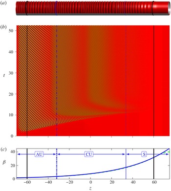
Numerical simulations for $\unicode[STIX]{x1D702}=0.85$ , $\mathit{Ta}=120$ with fluid injection. (a) Isosurface where the total azimuthal velocity is equal to one half of the velocity at the rotating inner cylinder, at final time. (b) Spatio-temporal diagram of the radial velocity at mid-gap $U(r_{mid},z,t)$ . (c) Axial Reynolds number $\unicode[STIX]{x1D6FD}(z)$ : numerical (dashed light grey, green online, curve) and analytical (solid dark grey, blue online, curve), this latter reconstructed from expression (2.5) and numerical values of the mean axial flow at the boundaries between the inlet buffer and central domain and the central domain and outlet buffer. These boundaries are shown in solid black circles (in panel a) and vertical lines. The dash-dotted dark grey (blue online) circle (in panel a) and vertical line locate the absolute/convective boundary; and the dotted dark grey (blue online) circle (in panel a) and vertical line show the convectively unstable/stable boundary. Stable regions are labelled S, convectively unstable regions are labelled CU and absolutely unstable regions are labelled AU.

Perturbations to the base flow occur from a combination of the numerical noise occurring throughout the system at all time steps and a controlled perturbation applied at the inlet on the first four azimuthal modes of the axial component of the velocity (see (52) and (53) in Tilton et al. Reference Tilton, Serre, Martinand and Lueptow2014). In all cases but figure 15(b), the controlled perturbation is smoothly ramped up and down in time, starting at the initial time step and over a short duration $5/\mathit{Ta}$ (see (54) in Tilton et al. Reference Tilton, Serre, Martinand and Lueptow2014). For figure 15(b), the controlled perturbation is continuously applied as the sum of 50 random frequencies (see (55) in Tilton et al. Reference Tilton, Serre, Martinand and Lueptow2014). Simulations used a numerical domain decomposed into two central subdomains of length $L_{central}=2\times 60$ ( $L_{central}=2\times 65$ for cross-flow reversal in § 3.2.3), bounded by an inlet buffer $L_{in}=10$ and an outlet buffer $L_{out}=15$ . All simulations are integrated in time until a saturated state is achieved.

Figure 6.

Numerical and analytical results for $\unicode[STIX]{x1D702}=0.85$ , $\mathit{Ta}=114$ , with fluid injection. (a) Solid piecewise horizontal (red online) curve: dominant frequency $\unicode[STIX]{x1D714}_{max}(z)$ , exhibiting three steps at $\unicode[STIX]{x1D714}=7.50$ , 15.01 and 30.02 (with spectral resolution $\unicode[STIX]{x0394}\unicode[STIX]{x1D714}_{fft}=0.17$ ) to be compared with the dashed dark grey (blue online) horizontal line: $\unicode[STIX]{x1D714}_{crit}^{glob}=7.40$ . The dotted dark grey (blue online) curve in panel (a) shows the local frequency $\unicode[STIX]{x1D714}^{loc}(z)$ at $\mathit{Ta}=114$ . (b) Radial velocity at mid-gap $U(r_{mid},z)$ , at final time (solid black curve), enveloped by the amplitude $\Vert U_{mid}\Vert (z)$ computed from the temporal Hilbert transform (solid, red online, curve). The solid black, dash-dotted dark grey (blue online) and dotted dark grey (blue online) vertical lines are as in figure 5.

Figure 7.

Similar to figure 6, with $\mathit{Ta}=130$ . The dominant frequency $\unicode[STIX]{x1D714}_{max}(z)$ (solid, red online, piecewise horizontal curve in panel a) exhibits four steps at $\unicode[STIX]{x1D714}=7.55$ , 15.26, 30.51 and 61.03 (with $\unicode[STIX]{x0394}\unicode[STIX]{x1D714}_{fft}=0.21$ ), to be compared with the dashed dark grey (blue online) line: $\unicode[STIX]{x1D714}_{crit}^{glob}=7.40$ .

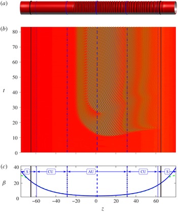
Typical results for simulations, performed at $\unicode[STIX]{x1D702}=0.85$ and $\mathit{Ta}=120$ with a short initial perturbation, are shown in figures 5 (fluid injection), 8 (fluid extraction) and 11 (cross-flow reversal). Panels (a) show snapshots, taken at the final simulation times, of the isosurfaces where the azimuthal velocity is 50 % that of the rotating cylinder, i.e., $0.5r_{1}\unicode[STIX]{x1D6FA}$ . The three configurations show the development of instabilities in the form of axisymmetric vortices. Panels (b) show spatio-temporal diagrams of the radial velocity at the mid-gap $U(r_{mid},z,t)$ . These show that in all three cases, the systems achieved saturated steady states in which vortices are present in only portions of the domains. In figures 5 and 11, the vortices tend to organize themselves in several packets, with different temporal frequencies. Following saturation, we compute these frequencies from the spatio-temporal diagrams by performing fast Fourier transforms (FFTs) in time at every axial location $z$ . Panels (a) of figures 6–7, 9–10 and 12–13 show the resulting dominant frequency $\unicode[STIX]{x1D714}_{max}(z)$ as solid (red online) piecewise horizontal lines. From the FFTs and related Hilbert transforms, we also demodulate the radial velocity at mid-gap. Panels (b) of the same figures show the resulting amplitudes $\Vert U_{mid}\Vert (z)$ in solid (red online) curves. We see that $\Vert U_{mid}\Vert (z)$ envelopes the solid black curve showing the instantaneous radial velocity at mid-gap at the final time.

Figure 8.

Similar to figure 5 ( $\unicode[STIX]{x1D702}=0.85$ and $\mathit{Ta}=120$ ), but for fluid extraction.

Figure 9.

Similar to figure 6, with $\unicode[STIX]{x1D702}=0.85$ , $\mathit{Ta}=113$ and fluid extraction. The dominant frequency $\unicode[STIX]{x1D714}_{max}(z)$ (solid piecewise horizontal, red online, curve in panel a) exhibits a single step at $\unicode[STIX]{x1D714}=7.69$ (with spectral resolution $\unicode[STIX]{x0394}\unicode[STIX]{x1D714}_{fft}=0.19$ ), to be compared with the dashed dark grey (blue online) horizontal line: $\unicode[STIX]{x1D714}_{crit}^{glob}=7.55$ and the dash-dotted light grey (green online) horizontal line: $\unicode[STIX]{x1D714}_{front}^{glob}=7.17$ . The solid black dotted and dash-dotted dark grey (blue online) vertical lines are as in figure 8. The dash-dotted light grey (green online) vertical line in panel (a) shows the modified front location $z_{front}^{glob}$ .

Figure 10.

Similar to figure 9 with $\mathit{Ta}=130$ . The dominant frequency $\unicode[STIX]{x1D714}_{max}(z)$ (solid piecewise horizontal, red online, curve in panel a) exhibits three steps at $\unicode[STIX]{x1D714}=18.45$ , 11.50 and 7.87 (with $\unicode[STIX]{x0394}\unicode[STIX]{x1D714}_{fft}=0.30$ ), to be compared with the dash-dotted horizontal dark grey (blue online) line: $\unicode[STIX]{x1D714}_{crit}^{glob}=7.55$ and the dash-dotted horizontal light grey (green online) line: $\unicode[STIX]{x1D714}_{front}^{glob}=17.91$ .

Figure 11.

As in figure 5 ( $\unicode[STIX]{x1D702}=0.85$ , $\mathit{Ta}=120$ ), for cross-flow reversal. The dashed dark grey, blue online, circle (in panel a) and vertical line locate the double turning point where the axial Reynolds number $\unicode[STIX]{x1D6FD}(z)$ is minimum.

Figure 12.

Similar to figure 6, with $\unicode[STIX]{x1D702}=0.85$ , $\mathit{Ta}=112$ and cross-flow reversal. The dominant frequency $\unicode[STIX]{x1D714}_{max}(z)$ (solid piecewise horizontal, red online, curve in panel a) exhibits two steps at $\unicode[STIX]{x1D714}=5.98$ and 11.96 (with spectral resolution $\unicode[STIX]{x0394}\unicode[STIX]{x1D714}_{fft}=0.24$ ), to be compared with the dashed dark grey (blue online) horizontal line: $\unicode[STIX]{x1D714}_{crit}^{glob}=6.04$ and the dash-dotted horizontal light grey (green online) line: $\unicode[STIX]{x1D714}_{front}^{glob}=6.00$ . The solid black, dashed, dash-dotted and dotted dark grey (blue online) vertical lines are as in figure 11. The dash-dotted light grey (green online) vertical line in panel (a) shows the modified front location $z_{front}^{glob}$ .

Figure 13.

Similar to figure 12 with $\mathit{Ta}=130$ . $\unicode[STIX]{x1D714}_{max}(z)$ (solid piecewise horizontal, red online, curve in panel a) exhibits six steps at $\unicode[STIX]{x1D714}=16.84$ , 10.32, 6.95, 13.89, 27.79 and 55.58 (with $\unicode[STIX]{x0394}\unicode[STIX]{x1D714}_{fft}=0.21$ ), to be compared with the dashed dark grey (blue online) horizontal line: $\unicode[STIX]{x1D714}_{crit}^{glob}=6.04$ and the dash-dotted light grey (green online) horizontal line: $\unicode[STIX]{x1D714}_{front}^{glob}=16.47$ .

3.2 Comparisons between numerical and analytical results

In this section, we use the global mode selection criteria presented in § 2 to analyse DNS results of systems characterized by fluid injection (figures 5–7), fluid extraction (figures 8–10) and cross-flow reversal (figures 11–13). For each case, we begin by extracting the axial variation of $\unicode[STIX]{x1D6FD}(z)$ from the DNS. To this we then fit the analytical expression (2.5) by evaluating the constants $A_{1}$ and $A_{2}$ using the mean axial flow in the DNS at the boundaries between the inlet and outlet buffers and the central subdomain. Panels (c) of figures 5 (fluid injection), 8 (fluid extraction) and 11 (cross-flow reversal) show there is excellent agreement between the DNS (dashed light grey, green online, curves) and expression (2.5) (solid dark grey, blue online, curves). The only deviation occurs in the inlet/outlet buffers (marked by solid vertical black lines in figures 5–13) where the permeability $\unicode[STIX]{x1D70E}$ of the DNS is smoothly set to zero.

Linear selection criteria are based on turning points located at minima of the axial Reynolds number $\unicode[STIX]{x1D6FD}(z)$ . For fluid injection (extraction), the minimum of $\unicode[STIX]{x1D6FD}(z)$ is located at the inlet (outlet), where, despite the buffer, the value obtained from expression (2.5) only minutely differs from the mean axial flow in the DNS. For cross-flow reversal, the location and value of the minimum of $\unicode[STIX]{x1D6FD}(z)$ are found from expression (2.5). As the permeability $\unicode[STIX]{x1D70E}$ does not appear in the local stability problem (B 2), the presence of the inlet/outlet buffers does not impact the local linear analysis of the perturbations, beyond setting $\unicode[STIX]{x1D6FD}(z)$ . The whole analysis is therefore based on the knowledge of the radius ratio $\unicode[STIX]{x1D702}$ , the permeability $\unicode[STIX]{x1D70E}$ , the mean axial flow at two locations and the Taylor number, together with resolutions of the local convective/absolute stability problem (B 2).

Boundaries where the flow transitions from stable to convectively unstable and from convectively unstable to absolutely unstable are found by solving the axially invariant stability problem (B 2) with $\mathit{Ta}$ as in the DNS, and $\unicode[STIX]{x1D6FD}$ so as to be at critical conditions for convective or absolute instabilities. Boundaries are then found as $z$ such that $\unicode[STIX]{x1D6FD}(z)$ in (2.5) is equal to the critical $\unicode[STIX]{x1D6FD}$ . In figures 5–13, stable regions are labelled convectively unstable regions are labelled and absolutely unstable regions are labelled When relevant, a double turning point is indicated by a dashed dark grey (blue online) vertical line, a boundary between a stable and convectively unstable domain by a dotted dark grey (blue online) vertical line and a boundary between a convectively and an absolutely unstable domain by a dash-dotted dark grey (blue online) vertical line in figures 5–13.

3.2.1 Fluid injection: maximum instability at the inlet

We begin by considering systems with fluid injection along the full length of the membrane. As demonstrated in figures 2(a) and 5(c), fluid injection causes the axial Reynolds number, $\unicode[STIX]{x1D6FD}(z)$ , to increase monotonically with $z$ , such that the local stability increases as fluid moves downstream. In the DNS, we impose fluid injection by applying $\unicode[STIX]{x1D6FD}_{inlet}=2$ and $\unicode[STIX]{x1D6FD}_{outlet}=40$ , for a permeability $\unicode[STIX]{x1D70E}=5\times 10^{-5}$ and $L_{central}=120$ . Simulations are repeated for $\mathit{Ta}=112$ , 114, 115, 120, 130, 140 and 150.

Figure 5 shows DNS results for $\mathit{Ta}=120$ . Panels (a,b) demonstrate that an axisymmetric instability develops and propagates from the inlet until it reaches a saturated state in which vortices are present over most of the domain, except near the outlet. From the spatio-temporal diagram in figure 5(b), we observe that the saturated state is characterized by vortices organized in several packets with different frequencies.

For fluid injection cases, our global mode analysis predicts a linear selection mechanism based on a simple turning point located at the inlet $z_{inlet}$ , as addressed in § 2.2.2. At leading order, based on the values of $\unicode[STIX]{x1D702}=0.85$ and $\unicode[STIX]{x1D6FD}_{inlet}=1.88$ , condition (2.18) and the resolution of the local stability problem (B 2) for absolute instability, with $\unicode[STIX]{x1D6FD}$ set to $\unicode[STIX]{x1D6FD}_{inlet}$ leads to a critical value $\mathit{Ta}_{crit}^{loc}=111.2$ , above which a global mode becomes unstable. Equation (2.19) predicts a corresponding critical frequency $\unicode[STIX]{x1D714}_{crit}^{loc}=6.87$ . Taking the corrections at the next order into account, expressions (2.21) and (2.22) slightly shift these values to $\mathit{Ta}_{crit}^{glob}=112.7$ , above which a global mode with frequency $\unicode[STIX]{x1D714}_{crit}^{glob}=7.40$ becomes unstable. The corrected critical Taylor number $\mathit{Ta}_{crit}^{glob}$ is in agreement with the DNS, which shows no instability at $\mathit{Ta}=112$ and an instability at $\mathit{Ta}=114$ .

Figure 6 shows the axial variations of the wavepacket in the DNS slightly above the critical conditions, at Taylor number $\mathit{Ta}=114$ . Figure 7 further departs from these critical conditions at $\mathit{Ta}=130$ . Global instabilities originating at the inlet occur in both cases. Near the inlet, these modes have the frequencies $\unicode[STIX]{x1D714}=7.50$ for $\mathit{Ta}=114$ and $\unicode[STIX]{x1D714}=7.55$ for $\mathit{Ta}=130$ . This is in agreement with the linear selection mechanism governed by a simple turning point at the inlet, leading to $\unicode[STIX]{x1D714}_{crit}^{glob}=7.40$ at critical conditions, as mentioned above. Nonlinear effects are expected in the dynamics of the instability, because the Taylor number departs from its critical value for a global mode, $\mathit{Ta}_{crit}^{glob}$ , in both DNS. The asymmetry between the inward ( $U(r_{mid},z,t_{final})<0$ ) and outward ( $U(r_{mid},z,t_{final})>0$ ) phases of the radial velocity observed in figures 6(b) and 7(b) tends to confirm the existence of noticeable nonlinearities that could also impact the frequency of the instability in the DNS. Such a modified frequency could be obtained using the nonlinear extension of semi-infinite global modes proposed in Couairon & Chomaz (Reference Couairon and Chomaz1997). The frequency, as measured in the leading subpacket of the DNS, nevertheless remains very close to the result of the linear selection mechanism.

Moving downstream from the inlet, the local dominant frequencies of the wavepackets in the DNS, $\unicode[STIX]{x1D714}_{max}(z)$ shown in figures 6(a) and 7(a) exhibit abrupt changes in a sequence of step-ups that are not accounted for by the global mode analysis. As indicated by the values in the captions of figures 6 and 7, these frequency jumps correspond to frequency doublings and occur until the wavepacket enters the locally stable domain and diminishes. Comparing the frequency jumps in figures 6(a) and 7(a) with the Hilbert transform in figures 6(b) and 7(b), we observe that the perturbation amplitude decreases as it approaches a frequency jump, and then increases downstream from the jump. These results suggest that the frequency jumps allow perturbations to resettle to more natural frequencies. This interpretation is supported by noting that the jumps occur both in the locally absolutely and convectively unstable regions, which suggests that the jumps are related to the local convective behaviour of the stability problem. The dotted dark grey (blue online) curves in figures 6(a) and 7(a) show the frequency $\unicode[STIX]{x1D714}^{loc}(z)$ of the most unstable axisymmetric convective mode obtained for the local axial Reynolds number $\unicode[STIX]{x1D6FD}(z)$ and the respective Taylor numbers. We see that frequency doublings occur at locations such that the local frequency coarsely adapts to $\unicode[STIX]{x1D714}^{loc}(z)$ . This feature will be further addressed in § 4.1.

3.2.2 Fluid extraction: maximum instability at the outlet

Next, we consider systems in which fluid is extracted along the full length of the membrane, as in figures 2(b) and 8(c). Fluid extraction causes $\unicode[STIX]{x1D6FD}(z)$ and the local stability of the flow to decrease monotonically as fluid moves downstream. In the DNS, we impose fluid extraction by applying $\unicode[STIX]{x1D6FD}_{inlet}=40$ and $\unicode[STIX]{x1D6FD}_{outlet}=2$ , for a permeability $\unicode[STIX]{x1D70E}=5\times 10^{-5}$ and $L_{central}=120$ . Simulations are repeated for $\mathit{Ta}=111$ , 113, 115, 120, 130 and 140.

Figure 8 shows DNS results for $\mathit{Ta}=120$ . We observe in figure 8(b) that an axisymmetric instability originates at the outlet. A wavepacket then propagates upstream until it reaches a steady state, within the region where the flow is locally absolutely unstable (downstream of the dash-dotted dark grey, blue online, vertical line). The spatio-temporal diagram in figure 8(b) shows that the steady wavepacket includes two subpackets, with different temporal frequencies.

For fluid extraction cases, our global mode analysis predicts a linear selection criterion based on the simple turning point at $z_{outlet}$ , described in § 2.2.2. For the values $\unicode[STIX]{x1D702}=0.85$ and $\unicode[STIX]{x1D6FD}_{outlet}=1.90$ , condition (2.18) predicts a critical value $\mathit{Ta}_{crit}^{loc}=111.4$ , above which a global mode becomes unstable. Equation (2.19) predicts the critical frequency $\unicode[STIX]{x1D714}_{crit}^{loc}=7.04$ . Considering the corrections at the next order, expressions (2.21) and (2.22) slightly shift these values to $\mathit{Ta}_{crit}^{glob}=112.3$ , above which a global mode with frequency $\unicode[STIX]{x1D714}_{crit}^{glob}=7.55$ becomes unstable. This linear critical condition $\mathit{Ta}_{crit}^{glob}$ is in agreement with DNS, which shows no instability at $\mathit{Ta}=111$ and an instability at $\mathit{Ta}=113$ .

In this configuration, global modes can also be governed by the nonlinear front-forming mechanism described in § 2.2.3. This possibility arises because the flow transitions from convectively unstable to absolutely unstable, at the axial locations $z_{c/a}$ indicated by the dash-dotted dark grey (blue online) vertical lines in figures 8, 9 and 10. At leading order, this mechanism selects the frequency $\unicode[STIX]{x1D714}_{front}^{loc}$ as the critical absolute frequency at $z_{c/a}$ , as given by (2.24). Implementing the next-order correction leads to the corrected frequency $\unicode[STIX]{x1D714}_{front}^{glob}$ computed from (2.25). This also shifts the front slightly downstream from $z_{c/a}$ to $z_{front}^{glob}$ , according to (2.26). Both the modified front location and selected frequency are then functions of the Taylor number and are shown in dash-dotted light grey (green online) vertical and horizontal lines, respectively, in figures 9 and 10.

Slightly above the critical conditions, at Taylor number $\mathit{Ta}=113$ (figure 9), the very good agreement between the linear frequency $\unicode[STIX]{x1D714}_{crit}^{glob}=7.55$ and the numerical result $\unicode[STIX]{x1D714}=7.69$ , together with the propagation of the perturbation upstream of the modified front location $z_{front}^{glob}$ , suggest that linear dynamics prevail for these weakly supercritical conditions.

Increasing the Taylor number further from critical conditions, to $\mathit{Ta}=130$ (figure 10), together with unshown results at $\mathit{Ta}=115$ , 120 and 140 exhibits the role of the nonlinear front-forming mechanism in the selection and dynamics of the global mode. The upstream edge of the perturbation in figure 10(b) almost exactly collapses on $z_{front}^{glob}$ (the dash-dotted light grey, green online, vertical line in figure 10 a) as given by (2.26). The frequency $\unicode[STIX]{x1D714}_{max}(z)=18.49$ of the leading subpacket agrees very well with $\unicode[STIX]{x1D714}_{front}^{glob}=17.91$ (the dash-dotted light grey, green online, horizontal line in figure 10 a) as given by (2.25).

Whereas the DNS at Taylor number $\mathit{Ta}=113$ in figure 9 shows a synchronized global mode, the DNS at $\mathit{Ta}=130$ in figure 10 shows that the local dominant frequency of the perturbation, $\unicode[STIX]{x1D714}_{max}(z)$ in figure 10(a), changes along the axial direction. This change takes the form of two successive jumps to smaller frequencies as fluid travels downstream across the wavepacket. As in § 3.2.1, this change is again associated with a ‘bump’ in the Hilbert transform shown in figure 10(b). This suggests again that the frequency jumps allow perturbations to resettle to more natural frequencies, depicted as the dotted (blue online) curves which show the frequency $\unicode[STIX]{x1D714}^{loc}(z)$ of the most unstable axisymmetric absolute mode obtained for the local axial Reynolds number $\unicode[STIX]{x1D6FD}(z)$ and the Taylor number of the DNS. Frequencies observed in figure 10 and for similar cases at $\mathit{Ta}=120$ and 140 suggests that the frequency downstream of the step-down is about two-thirds of the frequency upstream of the step-down. Section 4.1 will discuss these step-downs further.

3.2.3 Cross-flow reversal: maximum instability within the domain

Our final configuration considers systems with cross-flow reversal, as in figures 2(c) and 11(c). The axial Reynolds number first decreases with $z$ , then increases after the transmembrane flow reverses. This set-up exhibits a maximum of local instability where $\unicode[STIX]{x1D6FD}=\unicode[STIX]{x1D6FD}_{min}$ is a minimum. We impose cross-flow reversal in the DNS by applying $\unicode[STIX]{x1D6FD}_{inlet}=\unicode[STIX]{x1D6FD}_{outlet}=31.2$ , with a permeability $\unicode[STIX]{x1D70E}=2.3\times 10^{-4}$ and $L_{central}=130$ . Simulations are repeated for $\mathit{Ta}=110$ , 112, 115, 120, 130 and 140.

Figure 11 shows DNS results for $\mathit{Ta}=120$ . An axisymmetric instability develops in the form of a wavepacket originating slightly downstream from the location of $\unicode[STIX]{x1D6FD}_{min}$ (the dashed vertical dark grey, blue online, line), as seen in figure 11(b). This wavepacket propagates both down- and upstream until its trailing edge reaches the downstream stable domain (the dotted vertical dark grey, blue online, line on the right), where the instability diminishes, and its leading edge gets pinned downstream of the convective/absolute boundary (the dash-dotted vertical dark grey, blue online, line on the left). Figures 11(b,c) show that the steady wavepacket is again composed of several subpackets with different temporal frequencies.

A region of local absolute instability can exist around the location of $\unicode[STIX]{x1D6FD}_{min}$ . This location, where $\unicode[STIX]{x1D6FD}$ is minimum and the flow locally the most unstable, constitutes a double turning point. At leading order, from the minimum axial Reynolds number $\unicode[STIX]{x1D6FD}_{min}=1.61$ , the linear selection mechanism driven by the double turning point produces a critical Taylor number (2.13) $\mathit{Ta}_{crit}^{loc}=110.5$ and a critical frequency (2.14) $\unicode[STIX]{x1D714}_{crit}^{loc}=5.95$ . Including next-order corrections (2.16) and (2.17) shifts these slightly to $\mathit{Ta}_{crit}^{glob}=110.9$ and $\unicode[STIX]{x1D714}_{crit}^{glob}=6.04$ . The threshold for the instabilities in the DNS is in agreement with these analytical values. No instability is observed at $\mathit{Ta}=110$ , whereas increasing the Taylor number to $\mathit{Ta}=112$ exhibits an instability, as seen in figure 12.

Owing to the existence of the upstream convective/absolute boundary $z_{c/a}$ , the selection by the front-forming mechanism, described in § 2.2.3, may also occur, in a similar fashion to the cases of fluid extraction. As in § 3.2.2, both the modified front location, as given by (2.26), and selected frequency, as given by (2.25), are then functions of the Taylor number and are shown in dash-dotted light grey (green online) vertical and horizontal lines, respectively, in figures 12 and 13.

Slightly above the critical conditions, it is difficult to discern the selection mechanism of the global mode from the numerical simulation at $\mathit{Ta}=112$ in figure 12. The associated frequencies $\unicode[STIX]{x1D714}_{front}^{glob}=6.00$ by the nonlinear front and $\unicode[STIX]{x1D714}_{crit}^{glob}=6.04$ by the linear double turning point are nearly identical when $\mathit{Ta}=112$ , and are both close to the observed value $\unicode[STIX]{x1D714}=5.98$ for the leading subpacket. The fact that this subpacket does not exhibit a clear front could suggest a linear global mode, selected by the double turning point. The amplitude of such a linear global mode should grow until it reaches the downstream boundary between convectively unstable and stable domains, but in our case, such a growth is hampered by the local detuning and the frequency jump.

Increasing the Taylor number to $\mathit{Ta}=130$ in figure 13, together with unshown similar DNS at $\mathit{Ta}=115$ , 120 and 140, shows that the leading subpacket of the instability tends to be governed by the nonlinear front-forming mechanism, with this subpacket pinned on the shifted location $z_{front}^{glob}$ (the dash-dotted light grey, green online, vertical line in (a)) and the frequency of the subpacket $\unicode[STIX]{x1D714}=16.84$ closely matching the analytical value $\unicode[STIX]{x1D714}_{front}^{glob}=16.47$ (the dash-dotted light grey, green online, horizontal line in (a)) and clearly departing from $\unicode[STIX]{x1D714}_{crit}^{glob}=6.04$ .

As in §§ 3.2.1 and 3.2.2, the wavepackets at $\mathit{Ta}=112$ and 130 exhibit jumps in the dominant temporal frequency, $\unicode[STIX]{x1D714}_{max}(z)$ in (a), as fluid travels downstream. These jumps are similar to those observed in cases of fluid extraction, with step-downs upstream of the cross-flow reversal, and fluid injection, with step-ups downstream of the cross-flow reversal. As for fluid injection, figures 12 and 13, together with unshown results at $\mathit{Ta}=115$ , 120 and 140, show that step-ups consist of frequency doublings between the successive frequencies. In a fashion similar to fluid extraction, step-downs observed in figure 13 tend to follow a two-thirds ratio between the successive frequencies, though this is not as rigorous as the frequency doublings of the step-ups, and the lowest frequency $\unicode[STIX]{x1D714}=6.95$ is close to the frequency selected by a double turning point at the minimum of $\unicode[STIX]{x1D6FD}$ , $\unicode[STIX]{x1D714}_{crit}^{glob}=6.04$ . Those jumps are further addressed in the next section.

4 Discussion

4.1 The frequency jumps and the subpackets

For almost all cases, our DNS exhibit instabilities composed of several subpackets, oscillating at different temporal frequencies that occur in sequences of step-ups or step-downs. Step-ups are observed in regions of fluid injection as in the simulations of § 3.2.1, and in regions downstream of cross-flow reversal in § 3.2.3. Step-downs are observed in regions of fluid extraction, as in the simulations of § 3.2.2 and in regions upstream of cross-flow reversal in § 3.2.3. To investigate the dynamics of the subpackets and frequency jumps observed in our DNS, we consider the case of cross-flow reversal shown in figure 11 for $\mathit{Ta}=120$ . This set-up simultaneously presents step-ups and step-downs of the frequency. Further information can be obtained from figure 14, which shows the complete Fourier transform in time of the instability, upon which the computation of $\unicode[STIX]{x1D714}_{max}(z)$ is based, as a function of the axial coordinate $z$ .

Figure 14.

Frequency spectrum of the radial velocity at mid-gap obtained for cross-flow reversal at $\unicode[STIX]{x1D702}=0.85$ and $\mathit{Ta}=120$ , as in figure 11, as a function of the axial coordinate $z$ . The dash-dotted (green online) vertical line shows the location of the front $z_{front}^{glob}$ . The dashed (blue online) vertical line shows the location of the double turning point. The dotted (blue online) curve the local most amplified frequency $\unicode[STIX]{x1D714}^{loc}(z)$ .

Figure 15.

Numerical simulations for $\unicode[STIX]{x1D702}=0.85$ , $\mathit{Ta}=130$ with fluid extraction and the inlet locally convectively unstable. Radial velocity at mid-gap $U(r_{mid},z)$ , at final time (solid black curve) and amplitude computed from the temporal Hilbert transform (solid red curve). The perturbation at the inlet is at initial time (a) or a continuous random noise (b).

As seen in figure 14, as well as in figures 6–7 and 12–13, step-ups clearly consist of successive frequency doublings. These frequency doublings occur irrespective of whether the upstream subpacket with the lowest frequency was imposed by a linear turning point, as in § 3.2.1, or if it resulted from a sequence of step-downs upstream, as in the cross-flow reversal cases of § 3.2.3. This suggests that the frequency doubling is governed by some local dynamics. In figure 14, for example, the step-up between the two subpackets pulsating at frequencies $\unicode[STIX]{x1D714}_{2}$ and $2\unicode[STIX]{x1D714}_{2}$ occurs due to the local amplification in the subpacket downstream of the step-up of the first harmonic ( $2\unicode[STIX]{x1D714}_{2}$ ) of the frequency ( $\unicode[STIX]{x1D714}_{2}$ ) of the subpacket upstream of the step-up. The first harmonic ( $2\unicode[STIX]{x1D714}_{2}$ ) is fed by nonlinear dynamics and can be already observed in the subpacket upstream of the step-up. The frequency step-up occurs where this first harmonic is locally amplified by the mechanism of the centrifugal instability. This is shown by examining the local frequency $\unicode[STIX]{x1D714}^{loc}(z)$ , the dotted, blue online, curves in figures 14. Similar curves are also depicted in figures 6, 7, 12 and 13. This local frequency consists, in the domains where fluid injection occur and step-ups occur, of the frequency of the most unstable axisymmetric convective mode obtained at the local value of the axial Reynolds number $\unicode[STIX]{x1D6FD}(z)$ and the Taylor number of the DNS. The FFT depicted in figure 14 shows that, in the region of fluid injection, the maximum amplitudes of the successive harmonics are located along this curve of local frequency. As seen in figures 6, 7 and 12, in cases of fluid injection and cross-flow reversal close to the critical conditions, the instabilities consist in sequences of step-ups. It seems then legitimate to consider the complete wavepacket as a global mode: the leading subpacket subdues the successive downstream subpackets and, moreover, subpackets are synchronized, as harmonics are synchronized to their fundamental.

While step-ups can be explained in terms of local dynamics, a physical interpretation for the step-downs is more elusive. Step-downs occur when the leading subpacket is governed by the nonlinear front-forming mechanism at the convective/absolute boundary. In these cases, a linear turning point is also present downstream of the front, where the axial Reynolds number $\unicode[STIX]{x1D6FD}$ is minimum. In the simulations shown in figures 8, 10, 11, 13 and 14, the leading subpacket pulsates at the frequency $\unicode[STIX]{x1D714}_{front}^{glob}$ selected by the front (labelled $\unicode[STIX]{x1D714}_{1}$ in figure 14). The leading subpacket is superseded by a subpacket pulsating at a frequency close to $\unicode[STIX]{x1D714}_{crit}^{glob}$ selected by the linear turning point (labelled $\unicode[STIX]{x1D714}_{2}$ in figure 14). Furthermore, step-downs tend to follow a two-third ratio between the successive frequencies, though this ratio is not as rigorous as the frequency doublings observed in the step-ups. The step-down in figure 14 shows that the spatial overlap between the two subpackets involved, i.e. the $z$ -range where both frequencies are noticeably present, is limited. It is therefore not clear if, across a step-down, the upstream subpacket drives the downstream subpacket. This motivates us to compare the local maximum frequency $\unicode[STIX]{x1D714}_{max}(z)$ in regions where step-downs occur to a local frequency $\unicode[STIX]{x1D714}^{loc}(z)$ defined as the frequency of the most unstable axisymmetric absolute mode, obtained at the local axial Reynolds number $\unicode[STIX]{x1D6FD}(z)$ and the Taylor number of the DNS. This local frequency is shown as a dotted curve (blue online) in figures 10, 13 and 14. We observe that a new subpacket develops after a step-down where its frequency becomes the locally most unstable. In figure 14, the local frequency $\unicode[STIX]{x1D714}(z)$ of the DNS is compared to the analytical result $\unicode[STIX]{x1D714}^{loc}(z)$ . This latter is the frequency of the most unstable axisymmetric absolute mode where extraction and step-downs occur, while it is the frequency of the most unstable axisymmetric convective mode where injection and step-ups occur. This choice reflects the hypotheses that the perturbation downstream of a step-up is excited by the perturbation upstream, while the perturbation downstream of a step-down seems to arise irrespective of the perturbation upstream. Figure 3(b) suggests that convective and absolute frequencies weakly differ. Comparing the value of $\unicode[STIX]{x1D714}(z)$ to the local convective or absolute frequencies thus hardly discriminates between convective and absolute local dynamics of the perturbation.

Figure 16.

Numerical simulation for $\unicode[STIX]{x1D702}=0.85$ , $\mathit{Ta}=160$ with fluid injection: isosurface where the total azimuthal velocity is equal to one half of the velocity at the rotating inner cylinder, at final time. The whole domain is unstable and the dash-dotted (blue online) circle shows the absolute/convective boundary.

Though we found no convincing mechanisms that clearly explain the selection of the frequency drop in step-downs, we report some possibilities. First, we note that step-downs cannot be unambiguously explained by a downstream subpacket governed by a linear turning point superseding an upstream subpacket governed by the nonlinear front-forming mechanism. Figure 13, for instance, exhibits two successive step-downs involving three subpackets, one downstream of the front, one near the double turning point, and an intermediate one, the dynamics of which is unclear. A second hypothesis is motivated by the observation that successive frequencies in a step-down (labelled $\unicode[STIX]{x1D714}_{1}$ and $\unicode[STIX]{x1D714}_{2}$ in figure 14) are in a ratio close to two-thirds. This ratio suggest that the first harmonic ( $2\unicode[STIX]{x1D714}_{1}$ ) of the upstream subpacket excites the downstream subpacket via its second harmonic ( $3\unicode[STIX]{x1D714}_{2}$ ). Unfortunately, this ratio is only loosely matched and figure 14 reveals that this common harmonic $2\unicode[STIX]{x1D714}_{1}\approx 3\unicode[STIX]{x1D714}_{2}$ is weak. Third, a step-down could suggest that the locally most unstable absolute mode occurs along another branch of the dispersion relation. But the frequency of such a new branch would not conform to $\unicode[STIX]{x1D714}^{loc}(z)$ . Moreover, to date, no physically acceptable extra solution branches of absolute modes have been found for the dispersion relation. We cannot rule out, however, that an acceptable solution could exist, because finding extra pinch points in the complex $k$ -plane is difficult without an analytical expression for the dispersion relation. Finally, a step-down could be the symptom of a secondary instability. However, secondary instabilities in Taylor–Couette systems usually take the form of vortices presenting a waviness in the azimuthal direction, and the frequency of the subpacket downstream of a step-down would again not conform to the local frequency $\unicode[STIX]{x1D714}^{loc}(z)$ but to a different dispersion relation. Moreover, wavy vortices resulting from a secondary instability mechanism are observed in our DNS at higher Taylor numbers (see figure 16). Though we incline towards considering that the dynamics underlying the step-downs are intrinsic, i.e. the feature does not depend on external factors, they remain an open question. Related to these unsettled dynamics, to identify the whole wavepacket as a global mode is debatable.

4.2 The selection of the leading wavepackets

Besides the frequency jumps that cannot be explained in terms of global modes, the analysis presented § 2.2 leads to reliable and interesting results, summarized here. The thresholds in terms of $\mathit{Ta}_{crit}$ , beyond which instabilities develop in the DNS in § 3, agree with the analytical expressions based on a linear turning point, whether a simple turning point, as developed in § 2.2.2, in the case of fluid injection shown in § 3.2.1 and fluid extraction shown in § 3.2.2, or a double turning point, as developed in § 2.2.1, in the case of cross-flow reversal shown in § 3.2.3. The agreement is already satisfying with the leading order of the critical Taylor number $\mathit{Ta}_{crit}^{loc}$ as given by (2.13) and (2.18) and further improved when corrected to $\mathit{Ta}_{crit}^{glob}$ as given by (2.16) and (2.21). Concerning the frequency selection, the instabilities observed in the DNS are almost always composed of stacks of several subpackets of waves oscillating at different frequencies. Nevertheless, the leading subpackets always exhibit a frequency related to a global mode selection criterion. The linear selection by a simple turning point at the inlet (2.19) works accurately in the case of fluid injection, even when the Taylor number substantially departs from its critical value, and its dynamics downstream are clearly nonlinear, and without requiring to proceed to the next order (2.22). The linear selection by a simple turning point at the outlet (2.19) works accurately in the case of fluid extraction for Taylor numbers close to the critical conditions, as in figure 9, where, moreover, the instability is fully synchronized. The linear selection by a double turning point located where the axial Reynolds number $\unicode[STIX]{x1D6FD}(z)$ is minimum (2.14) works accurately in the case of cross-flow reversal for Taylor numbers close to the critical conditions, as in figure 12. For fluid extraction and cross-flow reversal, proceeding to the next orders (2.22) and (2.17) slightly improves those results.

As the Taylor number departs from the critical conditions, as in figures 10 and 13, the nonlinear selection by the front-forming mechanism accurately predicts the frequency and the location of the front of the leading subpacket in cases of fluid extraction and cross-flow reversal. This agreement, however, requires the corrected expressions (2.25) and (2.26). This mechanism is fully nonlinear, and the agreement between the DNS and the analysis actually improves as the Taylor number departs from its critical condition As the Taylor number increases, the front approaches to the absolute/convective boundary $z_{c/a}$ and the frequency approaches the leading-order expression (2.24).

The location and extension of the vortices in the domain can also be explained by the local analysis. In the case of fluid injection, the vortices develop between the inlet and the downstream boundary between the locally convectively unstable and stable regions (the dark grey, blue online, dashed vertical lines between the and regions). Entering the locally stable region they decayand vanish. In the case of fluid extraction, assuming that the front-forming mechanism selects the leading subpacket, the vortices develop between the upstream boundary between the locally convectively unstable and absolutely unstable regions (the dark grey, blue online, dashed vertical lines between the and regions) and the outlet. In the case of cross-flow reversal, assuming again that the leading subpacket is selected by the front-forming mechanism, the vortices develop between the upstream boundary between the convectively and absolutely unstable regions (the dark grey, blue online, dashed vertical lines between the and regions) and the downstream boundary between the locally convectively unstable and stable regions (the dark grey, blue online, dashed vertical lines between the and regions). Entering the locally stable region they decay and vanish.

4.3 How robust are the global modes?

In the DNS, the manner in which the flow is perturbed impacts the development of the vortices. In § 3, part of the perturbation is controlled as initial and/or boundary conditions, in the form of an initial non-axisymmetric perturbation of the axial component of the inlet velocity. The perturbation also includes numerical noise. Though very limited within the numerical subdomains of the multidomain simulations, some noticeable noise is expected at the boundaries between the subdomains, such as those between the inlet and outlet buffer and the central subdomain. Based on these different perturbations, we extrapolate that the initial perturbation at the inlet triggers the vortices in the case of fluid injection in § 3.2.1. The noise at the outlet triggers the vortices in the case of fluid extraction in § 3.2.2. The numerical noise in the whole domain triggers the vortices in the case of cross-flow reversal in § 3.2.3. The low level of this noise explains the longer time required to observe the instability in figure 11, compared to figures 5 and 8.

Different initial and/or boundary conditions could potentially lead to the selection of flow structures different from those we observed. Whereas the dynamics of the vortices observed in § 3 are based on local absolute instability, we now consider the possibility to observe structures driven by convective instabilities, in a fashion similar to the ‘convective route’ proposed to explain the transition to turbulence in the boundary layer over a rotating disk (see Imayama, Alfredsson & Lingwood Reference Imayama, Alfredsson and Lingwood2016, and references therein on this topic). In our case, these convective modes are conceived of as a response to a forcing in the form of a non-axisymmetric continuous random noise on the axial component of the velocity at the inlet, instead of an initial pulse. In the case of fluid extraction and cross-flow reversal, as shown in figures 8–10 and 11–13, respectively, the inlet is located in a locally stable domain, isolating the dynamics of the vortices from the perturbations at the inlet. We confirmed that changing the perturbation at the inlet from an initial pulse to a continuous random noise had no impact on the instabilities. In the case of fluid injection, as shown in figures 5–7, the minimum axial Reynolds number $\unicode[STIX]{x1D6FD}_{inlet}=2$ at the inlet implies that the location is convectively unstable as soon as $\mathit{Ta}>\mathit{Ta}_{crit}^{conv}\approx 108.5$ . Changing the perturbation at the inlet from an initial pulse to a continuous random noise results in identical steady wavepackets, similarly decomposed into sets of subpackets oscillating at the same frequencies $\unicode[STIX]{x1D714}_{max}(z)$ . The initially forced and continuously forced cases only differ by the fact that, in the latter case, the global mode rises from a substantial background noise resulting from the forcing of convective instabilities. The convective modes are therefore present in the flow, but the dynamics of the global mode prevail.

The possibility of triggering convective instabilities is further addressed in the case of fluid extraction at $\mathit{Ta}=130$ , by imposing a lower axial Reynolds number at the inlet $\unicode[STIX]{x1D6FD}_{inlet}=20$ , so that the inlet is now locally convectively unstable and by changing the inlet condition from an initial pulse to a continuous random noise. Figure 15 shows the results of these numerical simulations, with an initial perturbation (figure 15 a) or with a continuous random noise (figure 15 b) at the inlet. Whereas an initial perturbation evolves towards a leading subpacket governed by the front-forming mechanism, similar to the case shown in figure 10, a continuous noise leads to a more complex final steady wavepacket, the dynamics of which are hardly intelligible at this point, that could consist of convective instabilities upstream of the wavepacket. Despite these different upstream dynamics, the two downstream-most subpackets in both cases are of comparable axial extensions and frequencies, with $\unicode[STIX]{x1D714}=11.90$ and 8.28 for an initial perturbation (figure 15 a) and $\unicode[STIX]{x1D714}=12.18$ and 8.30 for a continuous noise (figure 15 b), probably denoting similar downstream dynamics related to the frequency step-downs addressed in § 4.1.

To investigate the sensitivity of the global modes to the numerical treatment of the DNS outlet conditions, we repeated all simulations shown in the current using a ‘sponge layer’ that attenuates perturbations in a near-outlet region (see Tilton et al. Reference Tilton, Serre, Martinand and Lueptow2014, for details). The results were qualitatively similar, except in cases of fluid extraction for which the sponge layer prevented the outlet from acting as a wavemaker. In this DNS, the flow was found to directly transition at $\mathit{Ta}=117$ to a global mode governed by a front forming at the boundary between the convectively unstable and absolutely unstable domains. Modifications of the outlet are known to impact the dynamics of instabilities in rotating-disk boundary layers (Pier Reference Pier2013; Appelquist et al. Reference Appelquist, Alfredsson, Schlatter and Lingwood2016), a configuration where the local instability increases with the radius, in a fashion similar to the increase of the instability along the axis in TCP with fluid extraction. The impact of the nature of the outlet on the instability in TCP flow would require a substantial and thorough study.

Another aspect of the robustness of these axisymmetric global modes is their stability with respect to azimuthal waviness. Axisymmetric Taylor vortices, stationary or travelling, are expected to acquire some azimuthal waviness as the Taylor number is increased (see Lueptow, Docter & Min Reference Lueptow, Docter and Min1992, for experimental results). In a Taylor–Couette flow without axial and radial through-flows, wavy vortices are expected above $\mathit{Ta}_{crit}^{wavy}\approx 120$ , for $\unicode[STIX]{x1D702}=0.85$ . In an axially varying configuration of fluid injection, these wavy vortices are observed in the numerical simulation at Taylor numbers $\mathit{Ta}=160$ , shown in figure 16. In the configurations of fluid extraction and cross-flow reversal, these wavy vortices have not been observed at $\mathit{Ta}=150$ , and no DNS at higher Taylor numbers are available so far. This discrepancy in the critical conditions for the occurrence of the azimuthal waviness could be accounted for by the finite axial extension of the vortex stack, more limited in the cases of fluid extraction and cross-flow reversal, that could hamper the azimuthal waviness, though this is only speculative.

5 Conclusions and outlook

We investigated hydrodynamic instabilities developing in an open Taylor–Couette cell with a permeable inner cylinder. Our methodology considered both global mode theory and DNS using high-order spectral methods. The study was motivated by applications to membrane separations and by elucidating the physics of instabilities developing over spatially varying flows in open systems. The global mode analysis proved challenging because the selection criteria available in the literature have seen little application to the full three-dimensional Navier–Stokes equations (see § 2.2). The numerical simulations were also challenging due to the membrane Darcy conditions on the permeable cylinder and the high aspect ratio domains (see § 3.1 and Tilton et al. Reference Tilton, Serre, Martinand and Lueptow2014). Our results nevertheless show that a global mode analysis based on the local linear dispersion relation successfully explains the critical conditions and locations of the instabilities observed in the DNS (see § 4.2). However, our DNS also clearly and reproducibly demonstrates a new feature of global modes to which we found no previous record in the literature. Specifically, the DNS produced global modes composed of stacked subpackets that are each synchronized at specific frequencies related to the spatial evolution of the most unstable local mode (see § 3.2). Cases in which the frequency steps up as one moves downstream between two subpackets can be explained by the local amplification of nonlinearly driven harmonics. A physical explanation for cases in which the frequency steps down, however, remains elusive (see § 4.1). We expect this new result will motivate future numerical and theoretical work to confirm and explain similar behaviours in other open systems with global modes.

As a final point and outlook, we consider how the mechanics of these instabilities could improve the design of rotating filtration devices. The set-up of such devices is similar to the case of fluid extraction, shown in § 3.2.2. The efficiency of rotating filtration is based on the idea that centrifugal instabilities, in the form of vortices, developing in the gap between the cylinders, will promote the mixing of the substance (whether a solute or a suspension) and thereby reduce the accumulation of the filtered retentate near the semi-permeable membrane surface. This reduces membrane fouling and improves performances. Crucial to the efficiency of rotating filtration devices is the transport and mixing of the solute or suspension by these vortices. These transport and mixing properties depend on the radial shape functions, temporal frequencies, wavenumbers and amplitude of the vortices in a complex fashion which is a current research topic for axially invariant configurations.

Figure 17.

Local linear stability results, as functions of the radius ratio $\unicode[STIX]{x1D702}$ and axial Reynolds number $\unicode[STIX]{x1D6FD}$ . (a) Convective critical Taylor number $\mathit{Ta}_{crit}^{conv}$ . (b) Absolute critical Taylor number $\mathit{Ta}_{crit}^{abs}$ . The colourscale of the surfaces corresponds to the critical azimuthal wavenumbers $n_{crit}^{conv}$ and $n_{crit}^{abs}$ . Solid (blue online) curve in (a) and dashed (blue online) curve in (b) show the specific results for convective and absolute, respectively, critical conditions at $\unicode[STIX]{x1D702}=0.85$ , as in figure 3.

Owing to the large number of physical and geometrical parameters, a parametric study of the flow and related transport and mixing in axially varying set-ups remains a tremendous task, if addressed experimentally or numerically. Analytical approaches can offer a way to reduce this task. Together with local convective/absolute stability analyses, the analytical framework of global modes helps foresee some aspects of the dynamics of the vortices, such as their critical conditions, frequencies and wavenumbers, and in the case of global modes, their axial location and extension. These characteristics are determined by controlled parameters such as the solvent viscosity, the permeability and rotation rate of the inner membrane, the inlet feed rate of the device and the working pressure inside the inner cylinder. By setting the base flow and performing a local linear stability analysis as presented in appendix B, the flow configuration is amenable to parametric studies.

Present DNS and analyses in § 3 have covered cases with $\unicode[STIX]{x1D702}=0.85$ . To illustrate the interest of a parametric study, figure 17 shows the effect of varying the radius ratio $\unicode[STIX]{x1D702}$ on the convective (figure 17 a) and absolute (figure 17 b) critical Taylor numbers, $\mathit{Ta}_{crit}^{conv}$ and $\mathit{Ta}_{crit}^{abs}$ , for the centrifugal instabilities, parametrized by the axial Reynolds number $\unicode[STIX]{x1D6FD}$ . Results for convective instabilities are reproduced from Martinand, Serre & Lueptow (Reference Martinand, Serre and Lueptow2017). By favouring the occurrence of vortices, moderate radius ratios $(\unicode[STIX]{x1D702}\sim 0.5)$ could increase the efficiency of filtration devices. Besides the critical Taylor numbers, the critical azimuthal wavenumbers $n_{crit}^{conv}$ and $n_{crit}^{abs}$ are also indicated in figure 17 by the colourscale; non-zero values denoting the selection of helical travelling vortices instead of toroidal ones. Depending on their respective efficiencies for mixing and transport, which remain to be assessed, fine tuning the physical parameters to select toroidal or helical vortices could be of practical interest for filtration. Figure 17(b) shows that for most of the radius ratios, the critical absolute instabilities remain toroidal. Helical absolute vortices, though, can be selected in a narrow band of the $\unicode[STIX]{x1D702}-\unicode[STIX]{x1D6FD}$ space, where $\unicode[STIX]{x1D702}$ is close to unity, i.e. in narrow gaps, where right-handed helical modes ( $n_{crit}^{abs}=-1$ ) are selected. In contrast, convective instabilities of figure 17(a) are found to select left-handed helical modes with azimuthal wavenumbers up to $n_{crit}^{conv}=22$ as $\unicode[STIX]{x1D6FD}$ increases over the same range. From the aspect of the azimuthal wavenumber, one might conclude that favouring convective instabilities instead of absolute ones present some interest.

Besides the selection of convective, absolute or global modes, DNS presented in § 3.2.2 show that the stack of vortices decomposes into several subpackets, with different temporal frequencies, axial wavenumbers and phase speeds and, consequently, different transport properties. Understanding and predicting the frequency jumps would be of clear practical interest, either to account for them in models of rotating filtration or to design systems that avoid them. We are currently working along these lines. Moreover, predicting the amplitude at saturation of the vortices remains a complex and open question. This amplitude varies in the axial direction, is impacted by the frequency jumps, and results from nonlinear dynamics that have not been address to date.

Appendix A. Axially varying base flow

As explained in Tilton et al. (Reference Tilton, Martinand, Serre and Lueptow2010), a base flow for the axially varying configuration obtained when the rotating inner cylinder is permeable while the stationary outer one is impermeable is obtained by an asymptotic expansion. This expansion requires one to assume that both the non-dimensional permeability $\sqrt{\unicode[STIX]{x1D70E}}$ and the pressure drop along the axial direction $\unicode[STIX]{x0394}P/\unicode[STIX]{x0394}z$ , primarily related to the axial flow, are small. The axially varying base flow is then obtained as an asymptotic expansion up to the second order in $\unicode[STIX]{x1D700}=\sqrt{\unicode[STIX]{x1D70E}}$ :

(A 1a-c )

$$\begin{eqnarray}U_{b}(r,z)=\displaystyle \frac{\text{d}\unicode[STIX]{x1D6FD}}{\text{d}z}u_{b}(r),\quad V_{b}(r,z)=\displaystyle \mathit{Ta}v_{b,0}(r)+\frac{\text{d}\unicode[STIX]{x1D6FD}}{\text{d}z}v_{b,1}(r)\quad \text{and}\quad W_{b}(r,z)=\displaystyle \unicode[STIX]{x1D6FD}(z)w_{b}(r),\end{eqnarray}$$

with the varying axial Reynolds number $\unicode[STIX]{x1D6FD}(z)$ as given in (2.5). According to the asymptotic expansion, the axial Reynolds number $\unicode[STIX]{x1D6FD}(z)$ is first order in $\unicode[STIX]{x1D700}$ , so that $U_{b}(r,z)$ is second order in $\unicode[STIX]{x1D700}$ , the first term in $V_{b}(r,z)$ is zeroth order while the second one is second order, and $W_{b}(r,z)$ is first order.

The radial shape functions in (A 1) read as

(A 2)

$$\begin{eqnarray}\displaystyle & \displaystyle v_{b,0}(r)=\displaystyle \frac{r_{1}r_{2}}{r_{2}^{2}-r_{1}^{2}}\left(\frac{r_{2}}{r}-\frac{r}{r_{2}}\right), & \displaystyle\end{eqnarray}$$

(A 3)

$$\begin{eqnarray}\displaystyle & \displaystyle w_{b}(r)=\displaystyle 2\frac{r_{2}^{2}\ln (r/r_{1})+r_{1}^{2}\ln (r_{2}/r)-r^{2}\ln (r_{2}/r_{1})}{(r_{1}^{2}+r_{2}^{2})\ln (r_{2}/r_{1})-r_{2}^{2}+r_{1}^{2}}, & \displaystyle\end{eqnarray}$$

(A 4)

$$\begin{eqnarray}\displaystyle & \displaystyle u_{b}(r)=\frac{1}{16\ln \unicode[STIX]{x1D702}}\left[\frac{C}{r}+2Ar\ln r+(2B-A)r+(\ln \unicode[STIX]{x1D702})r^{3}\right] & \displaystyle\end{eqnarray}$$

and

(A 5)

$$\begin{eqnarray}v_{b,1}(r)=\frac{r_{1}}{128A\ln \unicode[STIX]{x1D702}}\left[Er+\frac{F}{r}+8Cr\ln r+4Ar^{3}\ln r+(4B-5A)r^{3}+\frac{2}{3}(\ln \unicode[STIX]{x1D702})r^{5}\right]\!,\end{eqnarray}$$

where $A=r_{2}^{2}-r_{1}^{2}$ , $B=r_{1}^{2}\ln r_{2}-r_{2}^{2}\ln r_{1}$ , $C=Ar_{2}^{2}+r_{2}^{4}\ln \unicode[STIX]{x1D702}$ ,

(A 6)

$$\begin{eqnarray}\displaystyle & \displaystyle D=\frac{r_{1}^{2}r_{2}^{2}}{2A^{2}}(\unicode[STIX]{x1D702}^{2}+\unicode[STIX]{x1D702}^{-2}-4\ln r_{1}), & \displaystyle\end{eqnarray}$$

(A 7)

$$\begin{eqnarray}\displaystyle & \displaystyle E=-8\frac{C}{A}(r_{2}^{2}\ln r_{2}-r_{1}^{2}\ln r_{1})+\frac{10\ln \unicode[STIX]{x1D702}}{3}(r_{1}^{4}+r_{1}^{2}r_{2}^{2}+r_{2}^{4})+5(r_{2}^{4}-r_{1}^{4}) & \displaystyle\end{eqnarray}$$

and

(A 8)

$$\begin{eqnarray}F=-r_{1}^{2}r_{2}^{2}\left[8\frac{C}{A}\ln \unicode[STIX]{x1D702}+\frac{10\ln \unicode[STIX]{x1D702}}{3}(r_{1}^{2}+r_{2}^{2})+5A\right]\!.\end{eqnarray}$$

Since the pressure field of the base flow is not required for the stability analysis, it is not included here.

Appendix B. Local convective/absolute stability analysis

The local linear convective/absolute stability analysis is similar to that in Martinand et al. (Reference Martinand, Serre and Lueptow2009), and is only summarized here. The velocity and pressure fields are decomposed as $[\boldsymbol{V},P]=[\boldsymbol{V}_{b}^{inv},P_{b}^{inv}]+[\boldsymbol{V}_{p}^{inv},P_{p}^{inv}]$ , where $\boldsymbol{V}_{b}^{inv}(r)=(0,\mathit{Ta}v_{b,0}(r),\unicode[STIX]{x1D6FD}w_{b}(r))^{t}$ is the axially invariant TCP base flow, quantified by Taylor number $\mathit{Ta}$ and constant axial Reynolds number $\unicode[STIX]{x1D6FD}$ , and $[\boldsymbol{V}_{p}^{inv}(r,\unicode[STIX]{x1D703},z,t),P_{p}^{inv}(r,\unicode[STIX]{x1D703},z,t)]$ is a small time-dependent perturbation. Equations (2.3) and (2.4) are linearized about the base flow $\boldsymbol{V}_{b}^{inv}$ , and the perturbation is sought as

(B 1)

$$\begin{eqnarray}[\boldsymbol{V}_{p}^{inv},P_{p}^{inv}]=[\boldsymbol{v}_{p}(r),p_{p}(r)]\exp (\text{i}\unicode[STIX]{x1D713})\quad \text{with}~\unicode[STIX]{x1D713}=kz+n\unicode[STIX]{x1D703}-\unicode[STIX]{x1D714}t,\end{eqnarray}$$

where $\unicode[STIX]{x1D714}$ is the temporal frequency, $k$ the axial wavenumber, and $n$ the azimuthal wavenumber. This yields an eigensystem of $r$ -differential equations satisfied by the radial shape functions $[\boldsymbol{v}_{p}(r),p_{p}(r)]$ , written in condensed form as:

(B 2)

$$\begin{eqnarray}\unicode[STIX]{x1D63C}(k,n,\boldsymbol{V}_{b}^{inv}(r))[\boldsymbol{v}_{p},p_{p}]=\unicode[STIX]{x1D714}\unicode[STIX]{x1D63D}[\boldsymbol{v}_{p},p_{p}],\end{eqnarray}$$

for which $[\boldsymbol{v}_{p}(r),p_{p}(r)]$ is an eigenvector and $\unicode[STIX]{x1D714}$ the associated eigenvalue. Operators $\unicode[STIX]{x1D63C}$ and $\unicode[STIX]{x1D63D}$ can be obtained in appendix B of Martinand et al. (Reference Martinand, Serre and Lueptow2017). System (B 2) is solved for a given set of parameters $(\mathit{Ta},\unicode[STIX]{x1D6FD},\unicode[STIX]{x1D702},k,n)$ using a Chebyshev spectral method. The solvability conditions of the set of systems of differential equations obtained by differentiating (B 2) with respect to $k$ , $n$ and the parameters $\mathit{Ta}$ and $\unicode[STIX]{x1D6FD}$ lead to the several partial derivatives of the complex frequency $\unicode[STIX]{x1D714}$ required by the convective/absolute stability analysis and the global mode selection criteria (besides the axial group velocity $\unicode[STIX]{x2202}_{k}\unicode[STIX]{x1D714}$ , $\unicode[STIX]{x2202}_{n}\unicode[STIX]{x1D714}$ , $\unicode[STIX]{x2202}_{\mathit{Ta}}\unicode[STIX]{x1D714}$ , $\unicode[STIX]{x2202}_{\unicode[STIX]{x1D6FD}}\unicode[STIX]{x1D714}$ , $\unicode[STIX]{x2202}_{k}^{2}\unicode[STIX]{x1D714}$ , $\unicode[STIX]{x2202}_{n}^{2}\unicode[STIX]{x1D714}$ and $\unicode[STIX]{x2202}_{k}\unicode[STIX]{x2202}_{n}\unicode[STIX]{x1D714}$ are also used in the analysis), and the corresponding partial derivatives of the eigenvector. As detailed in Martinand et al. (Reference Martinand, Serre and Lueptow2009), critical conditions $(k_{crit}^{conv},n_{crit}^{conv},\mathit{Ta}_{crit}^{conv})$ for the most unstable convective mode $([\boldsymbol{v}_{crit}^{conv},p_{crit}^{conv}],\unicode[STIX]{x1D714}_{crit}^{conv})$ are found by imposing $\text{Im}(\unicode[STIX]{x1D714})=0$ and $\text{Im}(\unicode[STIX]{x2202}_{k}\unicode[STIX]{x1D714})=0$ , with $k$ real and $n$ integer. Critical conditions $(k_{crit}^{abs},n_{crit}^{abs},\mathit{Ta}_{crit}^{abs})$ for the most unstable absolute mode $([\boldsymbol{v}_{crit}^{abs},p_{crit}^{abs}],\unicode[STIX]{x1D714}_{crit}^{abs})$ are found by imposing $\text{Im}(\unicode[STIX]{x1D714})=0$ and $\unicode[STIX]{x2202}_{k}\unicode[STIX]{x1D714}=0$ , with $k$ complex and $n$ integer. Those critical conditions and modes are found as functions of the other parameters $\unicode[STIX]{x1D6FD}$ and $\unicode[STIX]{x1D702}$ , as shown in figures 3 and 17.

References

Altmeyer, S., Hoffmann, Ch. & Lücke, M. 2011 Islands of instability for growth of spiral vortices in the Taylor–Couette system with and without axial through flow. Phys. Rev. E 84, 046308.Google Scholar

Appelquist, E., Alfredsson, P., Schlatter, P. H. & Lingwood, R. J. 2016 On the global nonlinear instability of the rotating-disk flow over a finite domain. J. Fluid Mech. 803, 332–355.Google Scholar

Appelquist, E., Schlatter, P. H., Alfredsson, P. & Lingwood, R. J. 2015 Global linear instability of the rotating-disk flow investigated through simulations. J. Fluid Mech. 765, 612–631.Google Scholar

Babcock, K. L., Ahlers, G. & Cannell, D. S. 1991 Noise-sustained structure in Taylor–Couette flow with through-flow. Phys. Rev. Lett. 67, 3388–3391.Google Scholar

Babcock, K. L., Ahlers, G. & Cannell, D. S. 1994 Noise amplification in open Taylor–Couette flow. Phys. Rev. E 50 (5), 3670–3692.Google Scholar

Beaudoin, G. & Jaffrin, M. Y. 1989 Plasma filtration in Couette flow membrane devices. Artif. Organs 13 (1), 43–51.Google Scholar

Büchel, P., Lücke, M., Roth, D. & Schmitz, R. 1996 Pattern selection in the absolutely unstable regime as a nonlinear eigenvalue problem: Taylor vortices in axial flow. Phys. Rev. E 53 (5), 4764–4776.Google Scholar

Carrière, Ph. & Monkewitz, P. A. 2001 Transverse-roll global modes in a Rayleigh–Bénard–Poiseuille convection. Eur. J. Mech. (B/Fluids) 20, 751–770.Google Scholar

Chomaz, J.-M. 2005 Global instabilities in spatially developing flows: non-normality and nonlinearity. Annu. Rev. Fluid Mech. 37, 357–392.Google Scholar

Chomaz, J.-M. & Couairon, A. 1999 Against the wind. Phys. Fluids 11 (10), 2977–2983.Google Scholar

Chung, K. C. & Astill, K. N. 1977 Hydrodynamic instability of viscous flow between rotating coaxial cylinders with fully developed axial flow. J. Fluid Mech. 81, 641–655.Google Scholar

Cotrell, D. L. & Pearlstein, A. J. 2004 The connection between centrifugal instability and Tollmien–Schlichting-like instability for spiral Poiseuille flow. J. Fluid Mech. 509, 331–351.Google Scholar

Couairon, A. & Chomaz, J.-M. 1997 Absolute and convective instabilities, front velocities and global modes in nonlinear systems. Physica D 108, 236–276.Google Scholar

Dee, G. & Langer, J. 1983 Propagating pattern selection. Phys. Rev. Lett. 50, 383–386.Google Scholar

DiPrima, R. C. 1960 The stability of a viscous fluid between rotating cylinders with an axial flow. J. Fluid Mech. 9, 621–631.Google Scholar

Donnelly, R. J. & Fultz, D. 1960 Experiments on the stability of spiral flow between rotating cylinders. Proc. Natl Acad. Sci. USA 46, 1150–1154.Google Scholar

Grandjean, E. & Monkewitz, P. A. 2009 Experimental investigation into localized instabilities of mixed Rayleigh–Bénard–Poiseuille convection. J. Fluid Mech. 640, 401–419.Google Scholar

Hallström, B. & Lopez-Leiva, M. 1978 Decription of a rotating ultrafiltration module. Desalination 24 (1–3), 273–279.Google Scholar

Healey, J. J. 2010 Model for unstable global modes in rotating-disk boundary layer. J. Fluid Mech. 663, 148–159.Google Scholar

Huerre, P. 2000 Open shear flow instabilities. In Perspectives in Fluid Dynamics (ed. Batchelor, G. K., Moffatt, H. K. & Worster, M. G.), pp. 159–229. Cambridge University Press.Google Scholar

Huerre, P. & Monkewitz, P. A. 1985 Absolute and convective instabilities in free shear layers. J. Fluid Mech. 159, 151–168.Google Scholar

Huerre, P. & Monkewitz, P. A. 1990 Local and global instabilities in spatially developing flows. Annu. Rev. Fluid Mech. 22, 473–537.Google Scholar

Imayama, S., Alfredsson, P. H. & Lingwood, R. J. 2016 Experimental study of rotating-disk boudary-layer flow with surface roughness. J. Fluid Mech. 786, 5–28.Google Scholar

Johnson, E. C. & Lueptow, R. M. 1997 Hydrodynamic stability of flow between rotating porous cylinders with radial and axial flow. Phys. Fluids 9 (12), 3687–3696.Google Scholar

Koshmieder, E. L. 1993 Bénard Cells and Taylor Vortices. Cambridge University Press.Google Scholar

Lee, S. & Lueptow, R. M. 2004 Rotating membrane filtration and rotating reverse osmosis. J. Chem. Engng Japan 37 (4), 471–482.Google Scholar

Lueptow, R. M., Docter, A. & Min, K. 1992 Stability of axial flow in an annulus with a rotating inner cylinder. Phys. Fluids A 4 (11), 2446–2455.Google Scholar

Martinand, D., Carrière, Ph. & Monkewitz, P. A. 2006 Three-dimensional global instability modes associated with a localized hot spot in Rayleigh–Bénard–Poiseuille convection. J. Fluid Mech. 551, 275–301.Google Scholar

Martinand, D., Serre, E. & Lueptow, R. M. 2009 Absolute and convective instability of cylindrical Couette flow with axial and radial flows. Phys. Fluids 21, 104102.Google Scholar

Martinand, D., Serre, E. & Lueptow, R. M. 2017 Weakly nonlinear analysis of cylindrical Couette flow with axial and radial flows. J. Fluid Mech. 824, 438–476.Google Scholar

Meseguer, A. & Marques, F. 2002 On the competition between centrifugal and shear instability in spiral Poiseuille flow. J. Fluid Mech. 455, 129–148.Google Scholar

Monkewitz, P. A., Huerre, P. & Chomaz, J.-M. 1993 Global linear stability analysis of weakly non-parallel shear flows. J. Fluid Mech. 288, 1–20.Google Scholar

Nicolas, X. 2002 Bibliographical review on the Poiseuille–Rayleigh–Bénard flows: the mixed convection flows in horizontal rectangular ducts heated from below. Intl J. Therm. Sci. 41 (10), 961–1016.Google Scholar

Pier, B. 2003 Finite-amplitude crossflow vortices, secondary instability and transition in the rotating-disk boundary layer. J. Fluid Mech. 487, 315–343.Google Scholar

Pier, B. 2013 Transition near the edge of a rotating disk. J. Fluid Mech. 737, R1.Google Scholar

Pier, B. & Huerre, P. 1996 Fully nonlinear global modes in spatially developing media. Physica D 97, 206–222.Google Scholar

Pier, B., Huerre, P. & Chomaz, J.-M. 2001 Bifurcation to fully nonlinear synchronized structures in slowly varying media. Physica D 148, 49–96.Google Scholar

Pier, B., Huerre, P., Chomaz, J.-M. & Couairon, A. 1998 Steep nonlinear global modes in spatially developing media. Phys. Fluids 10, 2433–2435.Google Scholar

Provansal, M., Mathis, C. & Boyer, L. 1987 Bénard–von Kármán instability: transient and forced regimes. J. Fluid Mech. 182, 1–22.Google Scholar

Rayleigh, Lord 1916 On convection currents in a horizontal layer of fluid when the higher temperature is on the under side. Phil. Mag. 32, 529–546.Google Scholar

Recktenwald, A., Lücke, M. & Müller, H. W. 1993 Taylor vortex formation in axial through-flow: linear and weakly nonlinear analysis. Phys. Rev. E 48 (6), 4444–4454.Google Scholar

van Saarloos, W. & Hohenberg, P. 1992 Fronts, pulses, sources and sinks in generalized complex Ginzburg–Landau equations. Physica D 56, 303–367.Google Scholar

Schwille, J. A., Mitra, D. & Lueptow, R. M. 2002 Design parameters for rotating filtration. J. Membr. Sci. 204 (1–2), 53–65.Google Scholar

Soward, A. M. & Jones, C. A. 1983 The linear stability of the flow in the narrow gap between two concentric rotating spheres. Q. J. Mech. Appl. Math. 36, 19–42.Google Scholar

Taylor, G. I. 1923 Stability of a viscous liquid contained between two rotating cylinders. Phil. Trans. R. Soc. Lond. A 223, 289–343.Google Scholar

Theofilis, V. 2003 Advances in global linear instability analysis of non-parallel and three-dimensional flows. Prog. Aerosp. Sci. 39, 289–315.Google Scholar

Tilton, N., Martinand, D., Serre, E. & Lueptow, R. M. 2010 Pressure-driven radial flow in a Taylor–Couette cell. J. Fluid Mech. 660, 527–537.Google Scholar

Tilton, N., Serre, E., Martinand, D. & Lueptow, R. M. 2014 A 3D pseudospectral algorithm for fluid flows with permeable walls. Application to filtration. Comput. Fluids 93, 129–145.Google Scholar

Figure 1.(a) Radial and axial velocities of the laminar base flow for the axially varying problem in a meridional plane. The outer cylinder is impermeable while fluid flows across the inner permeable cylinder, according to Darcy’s law, leading to a base flow varying along the axial direction. Panel (b) shows the azimuthal velocity of the base flow in an equatorial plane.

Figure 2.Three possible base flow variations of the axial Reynolds number $\unicode[STIX]{x1D6FD}(z)$ (solid lines) and radial Reynolds number $\unicode[STIX]{x1D6FC}_{1}(z)$ (dashed lines). (a) Results obtained when $\unicode[STIX]{x1D6FD}_{inlet}=2$, $\unicode[STIX]{x1D6FD}_{outlet}=40$ and $\unicode[STIX]{x1D70E}=5\times 10^{-5}$. The axial base flow $\unicode[STIX]{x1D6FD}(z)$ increases monotonically as fluid is injected along the membrane. The circle at the inlet marks the most unstable simple turning point as defined in § 2.2. (b) Results obtained when $\unicode[STIX]{x1D6FD}_{inlet}=40$, $\unicode[STIX]{x1D6FD}_{outlet}=2$ and $\unicode[STIX]{x1D70E}=5\times 10^{-5}$. The axial base flow $\unicode[STIX]{x1D6FD}(z)$ decreases monotonically as fluid is extracted along the membrane. The circle at the outlet marks the most unstable simple turning point as defined in § 2.2. (c) Results obtained when $\unicode[STIX]{x1D6FD}_{inlet}=20$, $\unicode[STIX]{x1D6FD}_{outlet}=20$ and $\unicode[STIX]{x1D70E}=2.3\times 10^{-4}$. The base flow $\unicode[STIX]{x1D6FD}(z)$ undergoes cross-flow reversal as $\unicode[STIX]{x1D6FC}_{1}(z)$ transitions from extraction to injection at $z=0$. The circle at the centre marks the most unstable double turning point as defined in § 2.2.

Figure 3.Local linear stability results for the critical convective (solid curves) and absolute (dashed curves) modes of instability, as functions of the axial Reynolds number $\unicode[STIX]{x1D6FD}$, for radius ratio $\unicode[STIX]{x1D702}=0.85$. (a) Critical Taylor numbers $\mathit{Ta}_{crit}^{conv}$ and $\mathit{Ta}_{crit}^{abs}$. (b) Critical frequencies $\unicode[STIX]{x1D714}_{crit}^{conv}$ and $\unicode[STIX]{x1D714}_{crit}^{abs}$. Digits in (a) indicate the azimuthal wavenumbers of the critical convective modes $n_{crit}^{conv}$.

Figure 4.Sketch of the numerical domain.

Figure 5.Numerical simulations for $\unicode[STIX]{x1D702}=0.85$, $\mathit{Ta}=120$ with fluid injection. (a) Isosurface where the total azimuthal velocity is equal to one half of the velocity at the rotating inner cylinder, at final time. (b) Spatio-temporal diagram of the radial velocity at mid-gap $U(r_{mid},z,t)$. (c) Axial Reynolds number $\unicode[STIX]{x1D6FD}(z)$: numerical (dashed light grey, green online, curve) and analytical (solid dark grey, blue online, curve), this latter reconstructed from expression (2.5) and numerical values of the mean axial flow at the boundaries between the inlet buffer and central domain and the central domain and outlet buffer. These boundaries are shown in solid black circles (in panel a) and vertical lines. The dash-dotted dark grey (blue online) circle (in panel a) and vertical line locate the absolute/convective boundary; and the dotted dark grey (blue online) circle (in panel a) and vertical line show the convectively unstable/stable boundary. Stable regions are labelled S, convectively unstable regions are labelled CU and absolutely unstable regions are labelled AU.

Figure 6.Numerical and analytical results for $\unicode[STIX]{x1D702}=0.85$, $\mathit{Ta}=114$, with fluid injection. (a) Solid piecewise horizontal (red online) curve: dominant frequency $\unicode[STIX]{x1D714}_{max}(z)$, exhibiting three steps at $\unicode[STIX]{x1D714}=7.50$, 15.01 and 30.02 (with spectral resolution $\unicode[STIX]{x0394}\unicode[STIX]{x1D714}_{fft}=0.17$) to be compared with the dashed dark grey (blue online) horizontal line: $\unicode[STIX]{x1D714}_{crit}^{glob}=7.40$. The dotted dark grey (blue online) curve in panel (a) shows the local frequency $\unicode[STIX]{x1D714}^{loc}(z)$ at $\mathit{Ta}=114$. (b) Radial velocity at mid-gap $U(r_{mid},z)$, at final time (solid black curve), enveloped by the amplitude $\Vert U_{mid}\Vert (z)$ computed from the temporal Hilbert transform (solid, red online, curve). The solid black, dash-dotted dark grey (blue online) and dotted dark grey (blue online) vertical lines are as in figure 5.

Figure 7.Similar to figure 6, with $\mathit{Ta}=130$. The dominant frequency $\unicode[STIX]{x1D714}_{max}(z)$ (solid, red online, piecewise horizontal curve in panel a) exhibits four steps at $\unicode[STIX]{x1D714}=7.55$, 15.26, 30.51 and 61.03 (with $\unicode[STIX]{x0394}\unicode[STIX]{x1D714}_{fft}=0.21$), to be compared with the dashed dark grey (blue online) line: $\unicode[STIX]{x1D714}_{crit}^{glob}=7.40$.

Figure 8.Similar to figure 5 ($\unicode[STIX]{x1D702}=0.85$ and $\mathit{Ta}=120$), but for fluid extraction.

Figure 9.Similar to figure 6, with $\unicode[STIX]{x1D702}=0.85$, $\mathit{Ta}=113$ and fluid extraction. The dominant frequency $\unicode[STIX]{x1D714}_{max}(z)$ (solid piecewise horizontal, red online, curve in panel a) exhibits a single step at $\unicode[STIX]{x1D714}=7.69$ (with spectral resolution $\unicode[STIX]{x0394}\unicode[STIX]{x1D714}_{fft}=0.19$), to be compared with the dashed dark grey (blue online) horizontal line: $\unicode[STIX]{x1D714}_{crit}^{glob}=7.55$ and the dash-dotted light grey (green online) horizontal line: $\unicode[STIX]{x1D714}_{front}^{glob}=7.17$. The solid black dotted and dash-dotted dark grey (blue online) vertical lines are as in figure 8. The dash-dotted light grey (green online) vertical line in panel (a) shows the modified front location $z_{front}^{glob}$.

Figure 10.Similar to figure 9 with $\mathit{Ta}=130$. The dominant frequency $\unicode[STIX]{x1D714}_{max}(z)$ (solid piecewise horizontal, red online, curve in panel a) exhibits three steps at $\unicode[STIX]{x1D714}=18.45$, 11.50 and 7.87 (with $\unicode[STIX]{x0394}\unicode[STIX]{x1D714}_{fft}=0.30$), to be compared with the dash-dotted horizontal dark grey (blue online) line: $\unicode[STIX]{x1D714}_{crit}^{glob}=7.55$ and the dash-dotted horizontal light grey (green online) line: $\unicode[STIX]{x1D714}_{front}^{glob}=17.91$.

Figure 11.As in figure 5 ($\unicode[STIX]{x1D702}=0.85$, $\mathit{Ta}=120$), for cross-flow reversal. The dashed dark grey, blue online, circle (in panel a) and vertical line locate the double turning point where the axial Reynolds number $\unicode[STIX]{x1D6FD}(z)$ is minimum.

Figure 12.Similar to figure 6, with $\unicode[STIX]{x1D702}=0.85$, $\mathit{Ta}=112$ and cross-flow reversal. The dominant frequency $\unicode[STIX]{x1D714}_{max}(z)$ (solid piecewise horizontal, red online, curve in panel a) exhibits two steps at $\unicode[STIX]{x1D714}=5.98$ and 11.96 (with spectral resolution $\unicode[STIX]{x0394}\unicode[STIX]{x1D714}_{fft}=0.24$), to be compared with the dashed dark grey (blue online) horizontal line: $\unicode[STIX]{x1D714}_{crit}^{glob}=6.04$ and the dash-dotted horizontal light grey (green online) line: $\unicode[STIX]{x1D714}_{front}^{glob}=6.00$. The solid black, dashed, dash-dotted and dotted dark grey (blue online) vertical lines are as in figure 11. The dash-dotted light grey (green online) vertical line in panel (a) shows the modified front location $z_{front}^{glob}$.

Figure 13.Similar to figure 12 with $\mathit{Ta}=130$. $\unicode[STIX]{x1D714}_{max}(z)$ (solid piecewise horizontal, red online, curve in panel a) exhibits six steps at $\unicode[STIX]{x1D714}=16.84$, 10.32, 6.95, 13.89, 27.79 and 55.58 (with $\unicode[STIX]{x0394}\unicode[STIX]{x1D714}_{fft}=0.21$), to be compared with the dashed dark grey (blue online) horizontal line: $\unicode[STIX]{x1D714}_{crit}^{glob}=6.04$ and the dash-dotted light grey (green online) horizontal line: $\unicode[STIX]{x1D714}_{front}^{glob}=16.47$.

Figure 14.Frequency spectrum of the radial velocity at mid-gap obtained for cross-flow reversal at $\unicode[STIX]{x1D702}=0.85$ and $\mathit{Ta}=120$, as in figure 11, as a function of the axial coordinate $z$. The dash-dotted (green online) vertical line shows the location of the front $z_{front}^{glob}$. The dashed (blue online) vertical line shows the location of the double turning point. The dotted (blue online) curve the local most amplified frequency $\unicode[STIX]{x1D714}^{loc}(z)$.

Figure 15.Numerical simulations for $\unicode[STIX]{x1D702}=0.85$, $\mathit{Ta}=130$ with fluid extraction and the inlet locally convectively unstable. Radial velocity at mid-gap $U(r_{mid},z)$, at final time (solid black curve) and amplitude computed from the temporal Hilbert transform (solid red curve). The perturbation at the inlet is at initial time (a) or a continuous random noise (b).

Figure 16.Numerical simulation for $\unicode[STIX]{x1D702}=0.85$, $\mathit{Ta}=160$ with fluid injection: isosurface where the total azimuthal velocity is equal to one half of the velocity at the rotating inner cylinder, at final time. The whole domain is unstable and the dash-dotted (blue online) circle shows the absolute/convective boundary.

Figure 17.Local linear stability results, as functions of the radius ratio $\unicode[STIX]{x1D702}$ and axial Reynolds number $\unicode[STIX]{x1D6FD}$. (a) Convective critical Taylor number $\mathit{Ta}_{crit}^{conv}$. (b) Absolute critical Taylor number $\mathit{Ta}_{crit}^{abs}$. The colourscale of the surfaces corresponds to the critical azimuthal wavenumbers $n_{crit}^{conv}$ and $n_{crit}^{abs}$. Solid (blue online) curve in (a) and dashed (blue online) curve in (b) show the specific results for convective and absolute, respectively, critical conditions at $\unicode[STIX]{x1D702}=0.85$, as in figure 3.

Article contents

Taylor–Couette–Poiseuille flow with a weakly permeable inner cylinder: absolute instabilities and selection of global modes

Abstract

JFM classification

Information

1 Introduction

2 Global modes in axially varying Taylor–Couette–Poiseuille flow

2.1 Base flow

2.2 Global modes and their selection mechanisms

2.2.1 Linear selection by a double turning point

2.2.2 Linear selection by a simple turning point

2.2.3 Nonlinear selection by the upstream convective/absolute boundary

3 Global modes in direct numerical simulations

3.1 Numerical method

3.2 Comparisons between numerical and analytical results

3.2.1 Fluid injection: maximum instability at the inlet

3.2.2 Fluid extraction: maximum instability at the outlet

3.2.3 Cross-flow reversal: maximum instability within the domain

4 Discussion

4.1 The frequency jumps and the subpackets

4.2 The selection of the leading wavepackets

4.3 How robust are the global modes?

5 Conclusions and outlook

Appendix A. Axially varying base flow

Appendix B. Local convective/absolute stability analysis

References

Save article to Kindle

Save article to Dropbox

Save article to Google Drive

Reply to: Submit a response

Your details

You have entered the maximum number of contributors

Conflicting interests