1 Introduction
Since the work of Rayleigh (Reference Rayleigh1878), it has been known that capillary jets are unstable to linear perturbations of wavelength longer than that of the circumference of the jet. This instability, referred to as the Plateau–Rayleigh instability, causes a capillary jet to break into droplets, and removes the possibility of the existence of steady solitary wave solutions. The steady solutions that do exist, that is periodic waves with wavelength shorter than the circumference of the jet, were computed numerically by Vanden-Broeck, Miloh & Spivack (Reference Vanden-Broeck, Miloh and Spivack1998). These waves, similar to the two-dimensional capillary waves found analytically by Crapper (Reference Crapper1957) for the case of infinite depth and Kinnersley (Reference Kinnersley1976) for finite depth, form overhanging structures as the amplitude increases, until finally a limiting configuration with a trapped bubble is formed. Alternatively, the solution branches can terminate on a non-trivial static configuration, where there is no motion in the fluid.
Ferrofluids are fluids containing nanoparticles of ferromagnetic material coated in molecular surfactant, resulting in the fluid having superparamagnetic behaviour. Ferrofluids are used in a variety of industrial applications, such as measuring the acceleration and inclination of oil drills, and sealing pump shafts (Raj, Moskowitz & Casciari Reference Raj, Moskowitz and Casciari1995). Since the analytic work and experiments of Bashtovoi & Krakov (Reference Bashtovoi and Krakov1978) and Arkhipenko et al. (Reference Arkhipenko, Barkov, Bashtovoi and Krakov1980), it has been known that magnetic fields can stabilise the Plateau–Rayleigh instability when considering a column of ferrofluid. This is done by coating a copper wire with ferrofluid and passing a current through the wire, inducing an azimuthal magnetic field. The buoyancy effects are suppressed by surrounding the ferrofluid in a non-magnetisable fluid of equal density. The problem is characterised by a magnetic Bond number
 $B$
, defined in § 2, which comes from a ratio of magnetic to capillary forces. Arkhipenko et al. (Reference Arkhipenko, Barkov, Bashtovoi and Krakov1980) show that when
 $B>1$
, the Rayleigh–Plateau instability is stabilised for all wavelengths. This formulation is of particular interest since it allows for axisymmetric solitary wave solutions. The axisymmetry makes the mathematical treatment of the problem significantly easier than that of a fully three-dimensional model, due to both the reduction in the number of free spatial variables, and the existence of a Stokes streamfunction (Batchelor Reference Batchelor1994, § 2.2).
In this paper, we consider two models. In the first model, named the one-layer model, we assume the surrounding non-magnetisable fluid has negligible density. In the second model, named the two-layer model, we consider a surrounding fluid of density equal to that of the ferrofluid. It is helpful to draw comparisons between the models discussed in this paper and the classical problem of two-dimensional gravity–capillary free-surface and interfacial waves. It is found there are many similarities, and some interesting differences, between these dispersive water wave systems. Reviews of two-dimensional gravity–capillary waves can be found in Dias & Kharif (Reference Dias and Kharif1999) and Vanden-Broeck (Reference Vanden-Broeck2010). We note that our model allows for variable density ratios of the two fluids. However, a ratio of unity is of particular interest since, as stated above, gravity free regimes can be experimentally realised this way. This was done recently by Bourdin, Bacri & Falcon (Reference Bourdin, Bacri and Falcon2010), where axisymmetric periodic and solitary waves were observed.
So far most analytic and numerical work on the problem has considered only the one-layer model. Under the assumption that the radius of the copper wire (denoted
 $d$
) is negligible, Rannacher & Engel (Reference Rannacher and Engel2006) derived a Korteweg–de Vries (KdV) equation to describe weakly nonlinear solitary waves. Like the KdV equation for gravity–capillary waves, it is found that for some critical values of the parameters, the coefficient of the dispersive term changes sign (Korteweg & de Vries Reference Korteweg and de Vries1895; Benjamin Reference Benjamin1982; Hunter & Vanden-Broeck Reference Hunter and Vanden-Broeck1983). For the ferromagnetic problem, this occurs at
 $B=B_{2}$
. However, unlike gravity–capillary waves, there is also a change in sign of the coefficient of the nonlinear term at
 $B=B_{1}<B_{2}$
. The implication is that the KdV equation predicts depression solitary waves in the region
 $B\in (B_{1},B_{2})$
, and elevation waves for
 $B\in (1,B_{1})$
and
 $B>B_{2}$
.
Blyth & Părău (Reference Blyth and Părău2014) (referred to as BP throughout) performed a numerical investigation of solitary wave solutions to the one-layer model in the fully nonlinear regime for arbitrary values of
 $d$
. They found that, for
 $1<B<B_{1}(d)$
, solitary waves bifurcating from zero amplitude are elevation waves, while for
 $B_{1}(d)<B<B_{2}(d)$
these solutions are depression waves. This is in good agreement with Rannacher & Engel’s KdV equation, who found
 $B_{1}=3/2$
and
 $B_{2}=9$
when
 $d=0$
. Time dependant computations on solutions of this type are considered by Guyenne & Părău (Reference Guyenne and Părău2016). Furthermore, BP also found branches of depression solitary waves bifurcating from non-zero amplitude for
 $1<B<B_{1}$
, and likewise elevation solitary waves bifurcating from non-zero amplitude for
 $B_{1}<B\leqslant 2$
. This is rather surprising, since such bifurcations have not been found for two-dimensional gravity–capillary waves.
For
 $B<B_{2}$
, the linear dispersion relation
 $c(k)$
is monotonic increasing, where
 $c$
is the wave speed and
 $k$
the wavenumber. When
 $B>B_{2}$
, a minimum appears. BP found no pure solitary waves (waves with monotonic decay in the far field) in this regime. They instead found solitary wave packets, which bifurcate from the minimum of the dispersion relation. These waves are described at small amplitude by a nonlinear Schrödinger equation, recently derived by Groves & Nilsson (Reference Groves and Nilsson2018) for the one-layer model under the assumption that
 $d=0$
. Groves and Nilsson also proved the existence of a variety of solitary wave solutions for this model. When there is a minimum, as well as solitary wave packets, one also expects to find generalised solitary waves. These are solitary waves characterised by a wave train of ripples in the far field. Such solutions have been found for gravity–capillary waves (for example, Hunter & Vanden-Broeck Reference Hunter and Vanden-Broeck1983). In this paper, we compute numerically solutions of this type for the ferrofluid jet. It is found that, for all parameter values tested, the far field of the solution is never flat along the branches of generalised solitary waves. This is checked by showing that the values of the curvature of the streamlines are non-zero in the far field. This was found to be the case for two-dimensional gravity–capillary waves in the numerical investigation of Champneys, Vanden-Broeck & Lord (Reference Champneys, Vanden-Broeck and Lord2002), and for hydroelastic waves by Gao & Vanden-Broeck (Reference Gao and Vanden-Broeck2014). Since no pure solitary waves are found when
 $B>B_{2}$
, the KdV equation does not accurately predict the behaviour of nonlinear solutions in this regime.
In this paper, we extend the numerical investigation of BP by computing generalised solitary waves and periodic waves for the one-layer model. Furthermore, we adapt the numerical method to allow for two flow domains, and compute solutions for the two-layer model. Steady periodic, solitary and generalised solitary wave solutions are found.
The paper is organised as follows. In § 2, we formulate the problem. In § 3, we derive the linear dispersion relation for the problem. In § 4, we describe the numerical method used to compute solutions. In § 5, the range of possible static solutions (
 $c=0$
) is discussed. In § 6, the results of the numerical investigation are presented. Section 7 is a conclusion to the paper.
2 Formulation
We consider an axisymmetric column of ferrofluid with constant density
 $\unicode[STIX]{x1D70C}_{1}$
and magnetic susceptibility
 $\unicode[STIX]{x1D712}_{1}$
, coating a copper rod of radius
 $d$
. We choose the cylindrical coordinate system
 $(x,r)$
such that
 $x$
points along the rod, and
 $r$
is the radial coordinate. The ferrofluid is surrounded by a non-magnetisable fluid (
 $\unicode[STIX]{x1D712}_{2}=0$
) of density
 $\unicode[STIX]{x1D70C}_{2}\leqslant \unicode[STIX]{x1D70C}_{1}$
(we do not consider values of
 $\unicode[STIX]{x1D70C}_{2}>\unicode[STIX]{x1D70C}_{1}$
to avoid the Rayleigh–Taylor instability). The interface is given by
 $r=\unicode[STIX]{x1D702}(x,t)$
, the mean radius of which is denoted
 $R$
. Denote the velocity fields in the ferrofluid and surrounding fluid as
 $\boldsymbol{u}_{1}=(u_{1},v_{1})$
and
 $\boldsymbol{u}_{2}=(u_{2},v_{2})$
in
 $(x,r)$
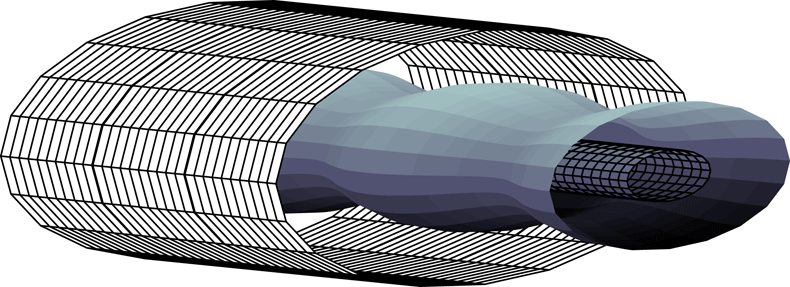
respectively. The system is contained inside a fixed cylindrical container of radius
 $D$
(see figures 1 and 2). We note that in the experiments of Arkhipenko et al. (Reference Arkhipenko, Barkov, Bashtovoi and Krakov1980) and Bourdin et al. (Reference Bourdin, Bacri and Falcon2010), the fluids were contained in a rectangular box. However, since axisymmetric interfaces were witnessed, the box must have been of a sufficient size to not destroy the axisymmetry of the problem. Therefore, comparison between the experiments and the model in this paper can be made by considering large values of
 $D$
.
A current
 $I$
is passed through the copper wire. This induces a purely azimuthal magnetic field, given by
 $$\begin{eqnarray}\boldsymbol{H}=\unicode[STIX]{x1D707}_{0}I/(2\unicode[STIX]{x03C0}r)\boldsymbol{e}_{\unicode[STIX]{x1D703}},\end{eqnarray}$$
where
 $\unicode[STIX]{x1D707}_{0}$
is the magnetic permeability in a vacuum, and
 $e_{\unicode[STIX]{x1D703}}$
is the unit vector in the clockwise azimuthal direction. We assume the linear magnetisation law, such that the magnetisation
 $\boldsymbol{M}$
satisfies
 $\boldsymbol{M}=\unicode[STIX]{x1D712}\boldsymbol{H}$
. The assumption of an axisymmetric interface results in the decoupling of the magnetic problem from the hydrodynamic problem (Rannacher & Engel Reference Rannacher and Engel2006). Continuity of pressure (Rosensweig Reference Rosensweig1985, § 5.1) on the interface is given by
 $$\begin{eqnarray}P_{1}=P_{2}+T\unicode[STIX]{x1D705}-\frac{\unicode[STIX]{x1D707}_{0}}{2}\unicode[STIX]{x1D712}^{2}(\boldsymbol{H}\boldsymbol{\cdot }\hat{\boldsymbol{n}}).\end{eqnarray}$$
Here,
 $P_{1}$
and
 $P_{2}$
are the pressures in the ferrofluid and outer fluid respectively,
 $T$
the surface tension, and
 $\unicode[STIX]{x1D705}$
the mean curvature, given by
 $$\begin{eqnarray}\unicode[STIX]{x1D705}=\frac{1}{\unicode[STIX]{x1D702}}\left(1+\left(\frac{\unicode[STIX]{x2202}\unicode[STIX]{x1D702}}{\unicode[STIX]{x2202}x}\right)^{2}\right)^{-1/2}-\frac{\unicode[STIX]{x2202}^{2}\unicode[STIX]{x1D702}}{\unicode[STIX]{x2202}x^{2}}\left(1+\left(\frac{\unicode[STIX]{x2202}\unicode[STIX]{x1D702}}{\unicode[STIX]{x2202}x}\right)^{2}\right)^{-3/2}.\end{eqnarray}$$
Note that since
 $\boldsymbol{H}$
is azimuthal, the pressure jump associated with the magnetic field is zero.
Formulation in cylindrical coordinates.

Three-dimensional visualisation of the problem.

We consider a wave of unchanging form with wavelength
 $\unicode[STIX]{x1D706}$
and celerity
 $c$
. Under the assumption that the flows in either region are irrotational and incompressible, both velocity fields can be written in terms of a velocity potential
 $\boldsymbol{u}_{1,2}=\unicode[STIX]{x1D735}\unicode[STIX]{x1D719}_{1,2}$
, where
 $\unicode[STIX]{x1D719}_{1}$
and
 $\unicode[STIX]{x1D719}_{2}$
satisfy the axisymmetric Laplace equation, given by
 $$\begin{eqnarray}\unicode[STIX]{x1D6FB}^{2}\unicode[STIX]{x1D719}_{i}=\frac{\unicode[STIX]{x2202}^{2}\unicode[STIX]{x1D719}_{i}}{\unicode[STIX]{x2202}r^{2}}+\frac{1}{r}\frac{\unicode[STIX]{x2202}\unicode[STIX]{x1D719}_{i}}{\unicode[STIX]{x2202}r}+\frac{\unicode[STIX]{x2202}^{2}\unicode[STIX]{x1D719}_{i}}{\unicode[STIX]{x2202}z^{2}}=0,\quad i=1,2,\end{eqnarray}$$
in their respective flow domains. We assume the wave is symmetric about the point
 $\unicode[STIX]{x1D719}_{1}=\unicode[STIX]{x1D719}_{2}=0$
. We require no normal flow through the rod and outer cylinder, that is
 $$\begin{eqnarray}\displaystyle & \displaystyle \frac{\unicode[STIX]{x2202}\unicode[STIX]{x1D719}_{1}}{\unicode[STIX]{x2202}r}=0\quad \text{for}~r=d, & \displaystyle\end{eqnarray}$$
 $$\begin{eqnarray}\displaystyle & \displaystyle \frac{\unicode[STIX]{x2202}\unicode[STIX]{x1D719}_{2}}{\unicode[STIX]{x2202}r}=0\quad \text{for}~r=D. & \displaystyle\end{eqnarray}$$
The Bernoulli principle (Rosensweig Reference Rosensweig1985, § 5.2) satisfied on the interface gives
 $$\begin{eqnarray}\frac{\unicode[STIX]{x2202}\unicode[STIX]{x1D719}_{1}}{\unicode[STIX]{x2202}t}-\unicode[STIX]{x1D70C}\frac{\unicode[STIX]{x2202}\unicode[STIX]{x1D719}_{2}}{\unicode[STIX]{x2202}t}+\frac{1}{2}(q_{1}^{2}-\unicode[STIX]{x1D70C}q_{2}^{2})+\frac{1}{\unicode[STIX]{x1D70C}_{1}}(P_{1}-P_{2})-\frac{\unicode[STIX]{x1D707}_{0}\unicode[STIX]{x1D712}_{1}I^{2}}{4\unicode[STIX]{x03C0}^{2}\unicode[STIX]{x1D70C}_{1}}\frac{1}{2r^{2}}={\hat{C}},\end{eqnarray}$$
where
 $q_{i}=|\unicode[STIX]{x1D735}\unicode[STIX]{x1D719}_{i}|$
,
 $\unicode[STIX]{x1D70C}=\unicode[STIX]{x1D70C}_{2}/\unicode[STIX]{x1D70C}_{1}$
and
 ${\hat{C}}$
is the Bernoulli constant. We take
 $R$
as the reference length and
 $\sqrt{T/(R\unicode[STIX]{x1D70C}_{1})}$
as the reference velocity. Making use of (2.2), we find that the non-dimensionalised Bernoulli equation is
 $$\begin{eqnarray}\frac{\unicode[STIX]{x2202}\unicode[STIX]{x1D719}_{1}}{\unicode[STIX]{x2202}t}-\unicode[STIX]{x1D70C}\frac{\unicode[STIX]{x2202}\unicode[STIX]{x1D719}_{2}}{\unicode[STIX]{x2202}t}+\frac{1}{2}(q_{1}^{2}-\unicode[STIX]{x1D70C}q_{2}^{2})+\unicode[STIX]{x1D705}-\frac{B}{2r^{2}}=C,\end{eqnarray}$$
where the magnetic Bond number
 $B$
is defined as
 $$\begin{eqnarray}B=\frac{\unicode[STIX]{x1D707}_{0}\unicode[STIX]{x1D712}_{1}I^{2}}{4\unicode[STIX]{x03C0}^{2}RT}.\end{eqnarray}$$
The magnetic Bond number is a ratio of magnetic to surface tension forces. It is shown in § 3 that the stability of linear perturbations is determined by
 $B$
. Finally, the kinematic boundary condition on the interface is given by
 $$\begin{eqnarray}\frac{\unicode[STIX]{x2202}\unicode[STIX]{x1D702}}{\unicode[STIX]{x2202}t}+\frac{\unicode[STIX]{x2202}\unicode[STIX]{x1D702}}{\unicode[STIX]{x2202}x}\frac{\unicode[STIX]{x2202}\unicode[STIX]{x1D719}_{i}}{\unicode[STIX]{x2202}x}=\frac{\unicode[STIX]{x2202}\unicode[STIX]{x1D719}_{i}}{\unicode[STIX]{x2202}r},\quad i=1,2.\end{eqnarray}$$
Note that for solitary waves with a flat far field, instead of fixing the mean of
 $\unicode[STIX]{x1D702}$
to unity, we fix
 $\unicode[STIX]{x1D702}$
in the far field to be unity. This choice of scaling gives rise to the far-field condition
 $$\begin{eqnarray}\unicode[STIX]{x1D702}\rightarrow 1,\quad \text{as}~x\rightarrow \pm \infty .\end{eqnarray}$$
It is left to solve the governing equation (2.4) for
 $\unicode[STIX]{x1D719}_{1}$
and
 $\unicode[STIX]{x1D719}_{2}$
in their respective flow domains, subject to boundary conditions, (2.5), (2.6), (2.8) and (2.10). We consider two values of
 $\unicode[STIX]{x1D70C}$
, that is
 $\unicode[STIX]{x1D70C}=0$
(one-layer model) and
 $\unicode[STIX]{x1D70C}=1$
(two-layer model). For the one-layer model, we ignore the outer boundary
 $r=D$
. This removes the requirement to solve for
 $\unicode[STIX]{x1D719}_{2}$
, since the equations concerning just
 $\unicode[STIX]{x1D719}_{1}$
form a closed system (no
 $\unicode[STIX]{x1D719}_{2}$
terms are present in (2.8) when
 $\unicode[STIX]{x1D70C}=0$
).
In the following section, we derive the linear dispersion relation for the system.
3 Linear theory
Consider a small perturbation to the uniform stream of the form
 $$\begin{eqnarray}\unicode[STIX]{x1D719}_{1}=\unicode[STIX]{x1D716}\mathop{\sum }_{m=1}^{\infty }F_{m}(r)\text{e}^{\text{i}mk(x-ct)},\quad \unicode[STIX]{x1D719}_{2}=\unicode[STIX]{x1D716}\mathop{\sum }_{m=1}^{\infty }G_{m}(r)\text{e}^{\text{i}mk(x-ct)},\end{eqnarray}$$
where
 $|\unicode[STIX]{x1D716}|\ll 1$
, and
 $F_{m}$
and
 $G_{m}$
are unknown functions of
 $r$
. Note that if
 $c^{2}>0$
, the solution is stable, while if
 $c^{2}<0$
, the amplitude grows exponentially in time and the solution is unstable. Ignoring terms of
 $O(\unicode[STIX]{x1D716}^{2})$
, and solving the linearised system, one finds the equation for the free surface,
 $$\begin{eqnarray}\unicode[STIX]{x1D702}=1+C_{1}\unicode[STIX]{x1D716}\left(\text{I}_{1}(k)-\frac{\text{I}_{1}(kd)}{\text{K}_{1}(kd)}\text{K}_{1}(k)\right)\text{e}^{\text{i}k(x-ct)}.\end{eqnarray}$$
Here,
 $\text{I}_{n}$
and
 $\text{K}_{n}$
are the modified Bessel functions of the first and second kind of order
 $n$
, and
 $C_{1}$
is an arbitrary constant. Equation (3.2) is a linear perturbation of wavenumber
 $k$
, travelling at speed
 $c$
. Furthermore, we recover the linear dispersion relation
 $$\begin{eqnarray}c^{2}=\frac{1}{\displaystyle k\left(\frac{m_{2}^{d}}{m_{1}^{d}}-\unicode[STIX]{x1D70C}\frac{m_{2}^{D}}{m_{1}^{D}}\right)}(k^{2}-1+B),\end{eqnarray}$$
where
 $$\begin{eqnarray}m_{1}^{d}=\text{I}_{1}(k)\text{K}_{1}(kd)-\text{K}_{1}(k)\text{I}_{1}(kd),\quad m_{2}^{d}=\text{I}_{0}(k)\text{K}_{1}(kd)+\text{I}_{1}(kd)\text{K}_{0}(k).\end{eqnarray}$$
Replacing all instances of
 $d$
with
 $D$
in the above equations gives
 $m_{1}^{D}$
and
 $m_{2}^{D}$
. If it is the case that
 $c(k)=c(nk)$
for some positive integer
 $n\geqslant 2$
, then the leading-order solution is given by
 $$\begin{eqnarray}\displaystyle \unicode[STIX]{x1D702} & = & \displaystyle 1+\unicode[STIX]{x1D716}C_{1}\left(\text{I}_{1}(k)-\frac{\text{I}_{1}(kd)}{\text{K}_{1}(kd)}\text{K}_{1}(k)\right)\text{e}^{\text{i}k(x-ct)}\nonumber\\ \displaystyle & & \displaystyle +\,\unicode[STIX]{x1D716}C_{n}\left(\text{I}_{1}(nk)-\frac{\text{I}_{1}(nkd)}{\text{K}_{1}(nkd)}\text{K}_{1}(nk)\right)\text{e}^{\text{i}nk(x-ct)}.\end{eqnarray}$$
This phenomenon is called Wilton ripples, and is only possible when a minimum occurs in the dispersion relation (corresponding to
 $B>B_{2}$
). A similar property is seen in gravity–capillary waves, and was originally derived by Wilton (Reference Wilton1915). One finds at higher order a solvability condition for
 $C_{n}$
. However, the algebra quickly becomes complicated, and instead these solutions are recovered via fully nonlinear computations, as seen in § 6.
Since
 $d<1<D$
and
 $0\leqslant \unicode[STIX]{x1D70C}\leqslant 1$
, the denominator in (3.3) is always positive, meaning that the stability of the solution depends on
 $k$
and
 $B$
. We find that solutions with wavenumber
 $k$
are stable if
 $$\begin{eqnarray}k^{2}>1-B.\end{eqnarray}$$
This is true for all
 $k$
if
 $B>1$
. Note that we recover the stability condition found by Rayleigh (Reference Rayleigh1878) by taking
 $B=0$
(that all solutions with
 $k<1$
are unstable).
The right-hand side of (3.3) tends to infinity as
 $k\rightarrow \infty$
. Hence, whether the dispersion curve has a minimum or not can be determined by considering the gradient of
 $c^{2}$
for small
 $k$
. A negative gradient for small
 $k$
corresponds to the existence of a minimum. Denoting the dispersion relation when
 $\unicode[STIX]{x1D70C}=0$
as
 $c_{\unicode[STIX]{x1D70C}}$
, we find that
 $$\begin{eqnarray}c_{\unicode[STIX]{x1D70C}}^{2}=\frac{1}{k}\left(\frac{m_{1}^{d}}{m_{2}^{d}}\right)(k^{2}-1+B).\end{eqnarray}$$
Taking a small
 $k$
expansion of the above equation, and differentiating with respect to
 $k$
, one gets
 $$\begin{eqnarray}2c_{\unicode[STIX]{x1D70C}}\frac{\text{d}c_{\unicode[STIX]{x1D70C}}}{\text{d}k}\approx \frac{1}{8}[(-1+4d^{2}-3d^{2}+4d^{4}\log d)(B-1)+8(1-d^{2})]k+O(k^{3}).\end{eqnarray}$$
Hence, there exists a minimum in
 $c_{\unicode[STIX]{x1D70C}}(k)$
given that the coefficient of
 $k$
in the above equation is negative. This is the case if
 $B>B_{2}$
, where
 $B_{2}$
has the following dependence on
 $d$
:
 $$\begin{eqnarray}B_{2}(d)=1+\frac{8(1-d^{2})}{1-4d^{2}+3d^{4}-4d^{4}\log d}.\end{eqnarray}$$
This expression is in agreement with (3.5) in the paper of BP. We see in § 6 that the characteristics of the solution space changes upon the existence of a minimum.
When
 $\unicode[STIX]{x1D70C}=1$
, we now expect
 $B_{2}$
to have dependence on both
 $d$
and
 $D$
. In the case when
 $D\rightarrow \infty$
, BP demonstrated that
 $B_{2}=1$
. For a finite value of
 $D$
, one can follow the same argument given above for
 $c_{\unicode[STIX]{x1D70C}}$
to find that
 $$\begin{eqnarray}B_{2}(d,D)=1-\frac{E}{F},\end{eqnarray}$$
where
 $$\begin{eqnarray}\displaystyle E & = & \displaystyle \frac{\frac{1}{2}(1-d^{2})(D^{2}-1)}{(D^{2}-1)+(1-d^{2})},\end{eqnarray}$$
 $$\begin{eqnarray}\displaystyle F & = & \displaystyle \frac{1}{8(D^{2}-d^{2})^{2}} [(D^{2}-1)(1-d^{2})(D-d)(D+d)+2d^{4}(D^{2}-1)^{2}\log d\nonumber\\ \displaystyle & & \displaystyle -\,2D^{4}(d^{2}-1)^{2}\log D].\end{eqnarray}$$
We will find it useful to denote the value of
 $c$
at
 $k=0$
as
 $c_{0}$
, and the minimum value of
 $c$
occurring at
 $k=k_{m}$
to be denoted
 $c_{m}$
. When
 $B<B_{2}$
,
 $c_{0}=c_{m}$
. In the following section, we describe the numerical method used to solve the fully nonlinear problem.
4 Numerical scheme
We consider a wave of wavelength
 $\unicode[STIX]{x1D706}$
travelling with unchanging form at a constant speed
 $c$
. We remove time dependence by taking a frame of reference travelling with the wave. We will use a finite difference scheme originally proposed by Woods (Reference Woods1951) for axisymmetric flows, and later independently formulated by Jeppson (Reference Jeppson1970). The method has since been used by a variety of authors for axisymmetric capillary waves (Vanden-Broeck et al.
Reference Vanden-Broeck, Miloh and Spivack1998) under the effect of electric (Grandison et al.
Reference Grandison, Vanden-Broeck, Papageorgiou, Miloh and Spivak2008) or magnetic (BP) fields, and the rise of Taylor bubbles in a tube (Doak & Vanden-Broeck Reference Doak and Vanden-Broeck2018). We will first describe the method used to find solutions to the two-layer model. This involves adapting the finite difference scheme to allow for two computational domains, as described below. Following this, we state the simplifications made to the method to solve the one-layer problem.
The idea is to solve the problem by finding the physical variable
 $r$
in the two potential spaces
 $(\unicode[STIX]{x1D719}_{1},\unicode[STIX]{x1D713}_{1})$
and
 $(\unicode[STIX]{x1D719}_{2},\unicode[STIX]{x1D713}_{2})$
, where
 $\unicode[STIX]{x1D713}_{1}$
and
 $\unicode[STIX]{x1D713}_{2}$
are the Stokes streamfunctions, defined by
 $$\begin{eqnarray}u_{i}=\frac{1}{r}\frac{\unicode[STIX]{x2202}\unicode[STIX]{x1D713}_{i}}{\unicode[STIX]{x2202}r},\quad v_{i}=-\frac{1}{r}\frac{\unicode[STIX]{x2202}\unicode[STIX]{x1D713}_{i}}{\unicode[STIX]{x2202}x},\quad i=1,2.\end{eqnarray}$$
Lines given by
 $\unicode[STIX]{x1D713}_{i}=$
constant are everywhere parallel to the velocity vector
 $\boldsymbol{u}_{i}$
, and are orthogonal to lines of constant
 $\unicode[STIX]{x1D719}_{i}$
. However, it is interesting to note that the Stokes streamfunction, unlike it’s two-dimensional counterpart, does not satisfy the Laplace equation. Therefore, the powerful tools of complex analysis are unavailable to us here, since the mapping from the
 $(x,r)$
space to the
 $(\unicode[STIX]{x1D719},\unicode[STIX]{x1D713})$
space is not conformal. Without loss of generality, we choose to define
 $\unicode[STIX]{x1D713}_{1}=d^{2}c/2=Q_{d}$
on
 $r=d$
,
 $\unicode[STIX]{x1D713}_{1}=\unicode[STIX]{x1D713}_{2}=Q$
on the interface, and
 $\unicode[STIX]{x1D713}_{2}=Q_{D}$
on
 $r=D$
. We note that, in the case of a flat free surface (uniform stream solution),
 $Q=c/2$
and
 $Q_{D}=cD^{2}/2$
. Integrating (4.1) with
 $u_{i}=c$
and
 $v_{i}=0$
, the uniform stream solution is found to be
 $$\begin{eqnarray}r=\left\{\begin{array}{@{}ll@{}}\displaystyle \sqrt{\frac{2\unicode[STIX]{x1D713}_{1}}{c}},\quad & \text{if }Q_{d}\leqslant \unicode[STIX]{x1D713}_{1}\leqslant Q,\\ \displaystyle \sqrt{\frac{2\unicode[STIX]{x1D713}_{2}}{c}},\quad & \text{if }Q<\unicode[STIX]{x1D713}_{2}\leqslant Q_{D}.\end{array}\right.\end{eqnarray}$$
This encourages the coordinate transformations
 $\unicode[STIX]{x1D713}_{1}=t^{2}$
and
 $\unicode[STIX]{x1D713}_{2}=s^{2}$
to better distribute streamlines between the interface and the boundaries. This choice of transformation means that taking equally spaced points in the discretisation of
 $t$
and
 $s$
results in equally spaced streamlines in the computation of the uniform stream solution. Seeking a periodic wave of wavelength
 $\unicode[STIX]{x1D706}$
, symmetric about
 $\unicode[STIX]{x1D719}_{1}=\unicode[STIX]{x1D719}_{2}=0$
, the ferrofluid and surrounding fluid flow domains are mapped onto the rectangular domains
 $\unicode[STIX]{x1D6FA}_{1}$
and
 $\unicode[STIX]{x1D6FA}_{2}$
respectively, where
 $$\begin{eqnarray}\displaystyle \unicode[STIX]{x1D6FA}_{1} & = & \displaystyle \{\unicode[STIX]{x1D719}_{1}\in [-c\unicode[STIX]{x1D706}/2,0],t\in [Q_{d}^{1/2},Q^{1/2}]\},\end{eqnarray}$$
 $$\begin{eqnarray}\displaystyle \unicode[STIX]{x1D6FA}_{2} & = & \displaystyle \{\unicode[STIX]{x1D719}_{2}\in [-c\unicode[STIX]{x1D706}/2,0],s\in [Q^{1/2},Q_{D}^{1/2}]\}.\end{eqnarray}$$
The two flow domains in potential space. The interface between the two fluids is in bold, and corresponds to the same streamline in physical space.

Here, we only consider the flow domains over half a wavelength, making use of the assumed symmetry. The flow domain in the potential space is shown in figure 3. Seeking
 $r$
as a function of the independent variables
 $(\unicode[STIX]{x1D719}_{1},\unicode[STIX]{x1D713}_{1})$
in
 $\unicode[STIX]{x1D6FA}_{1}$
and
 $(\unicode[STIX]{x1D719}_{2},\unicode[STIX]{x1D713}_{2})$
in
 $\unicode[STIX]{x1D6FA}_{2}$
, we find that (2.4) under the mapping becomes
 $$\begin{eqnarray}r^{3}\frac{\unicode[STIX]{x2202}^{2}r}{\unicode[STIX]{x2202}\unicode[STIX]{x1D713}_{i}^{2}}+r\frac{\unicode[STIX]{x2202}^{2}r}{\unicode[STIX]{x2202}\unicode[STIX]{x1D719}_{i}^{2}}+r^{2}\left(\frac{\unicode[STIX]{x2202}r}{\unicode[STIX]{x2202}\unicode[STIX]{x1D713}_{i}}\right)^{2}-\left(\frac{\unicode[STIX]{x2202}r}{\unicode[STIX]{x2202}\unicode[STIX]{x1D719}_{i}}\right)^{2}=0.\end{eqnarray}$$
Furthermore, one can express
 $q_{i}=|\unicode[STIX]{x1D735}\unicode[STIX]{x1D719}_{i}|$
and the mean curvature
 $\unicode[STIX]{x1D705}$
evaluated on the interface as functions of
 $\unicode[STIX]{x1D719}_{i}$
, using the identities
 $$\begin{eqnarray}\displaystyle & \displaystyle q_{i}(\unicode[STIX]{x1D719}_{i})=(u_{i}^{2}+v_{i}^{2})^{1/2}=\left(\left(\frac{\unicode[STIX]{x2202}r}{\unicode[STIX]{x2202}\unicode[STIX]{x1D719}_{i}}\right)^{2}+r^{2}\left(\frac{\unicode[STIX]{x2202}r}{\unicode[STIX]{x2202}\unicode[STIX]{x1D713}_{i}}\right)^{2}\right)^{1/2}, & \displaystyle\end{eqnarray}$$
 $$\begin{eqnarray}\displaystyle & \displaystyle \unicode[STIX]{x1D705}_{i}(\unicode[STIX]{x1D719}_{i})=-q_{i}^{3}\left(r\frac{\unicode[STIX]{x2202}r}{\unicode[STIX]{x2202}\unicode[STIX]{x1D713}_{i}}\frac{\unicode[STIX]{x2202}^{2}r}{\unicode[STIX]{x2202}\unicode[STIX]{x1D719}_{i}^{2}}-\left(\frac{\unicode[STIX]{x2202}r}{\unicode[STIX]{x2202}\unicode[STIX]{x1D719}_{i}}\right)^{2}\frac{\unicode[STIX]{x2202}r}{\unicode[STIX]{x2202}\unicode[STIX]{x1D713}_{i}}-r\frac{\unicode[STIX]{x2202}r}{\unicode[STIX]{x2202}\unicode[STIX]{x1D719}_{i}}\frac{\unicode[STIX]{x2202}^{2}r}{\unicode[STIX]{x2202}\unicode[STIX]{x1D719}_{i}\unicode[STIX]{x1D713}_{i}}\right)+\frac{\unicode[STIX]{x2202}r}{\unicode[STIX]{x2202}\unicode[STIX]{x1D713}_{i}}q_{i}. & \displaystyle\end{eqnarray}$$
Note that
 $\unicode[STIX]{x1D705}_{1}$
here denotes the mean curvature as a function of
 $\unicode[STIX]{x1D719}_{1}$
, and likewise for
 $\unicode[STIX]{x1D705}_{2}$
. These functions correspond to the same curve in physical space (the interface), and hence have the same value at given points along the interface, but are different functions due to the discontinuity in tangential velocities across the interface. We discretise
 $\unicode[STIX]{x1D6FA}_{1}$
and
 $\unicode[STIX]{x1D6FA}_{2}$
into equidistant points with
 $M$
points in
 $\unicode[STIX]{x1D719}_{1}$
and
 $\unicode[STIX]{x1D719}_{2}$
,
 $N$
points in
 $t$
and
 $P$
points in
 $s$
as follows
 $$\begin{eqnarray}\displaystyle & \displaystyle \unicode[STIX]{x1D719}_{1_{i}}=\unicode[STIX]{x1D719}_{2_{i}}=-\frac{c\unicode[STIX]{x1D706}}{2(M-1)}(M-i)\quad i=1,\ldots ,M, & \displaystyle\end{eqnarray}$$
 $$\begin{eqnarray}\displaystyle & \displaystyle t_{j}=Q_{d}^{1/2}+(Q^{1/2}-Q_{d}^{1/2})\frac{j-1}{N-1}\quad j=1,\ldots ,N, & \displaystyle\end{eqnarray}$$
 $$\begin{eqnarray}\displaystyle & \displaystyle s_{j}=Q^{1/2}+(Q_{D}^{1/2}-Q^{1/2})\frac{j-1}{P-1}\quad j=1,\ldots ,P. & \displaystyle\end{eqnarray}$$
We satisfy the governing equation (4.5) at the interior nodes of
 $\unicode[STIX]{x1D6FA}_{1}$
and
 $\unicode[STIX]{x1D6FA}_{2}$
, finding the values of derivatives with finite difference approximations. We use second-order central differences, making use of the symmetry by imposing
 $\unicode[STIX]{x2202}r/\unicode[STIX]{x2202}\unicode[STIX]{x1D719}_{i}=0$
at
 $\unicode[STIX]{x1D719}_{i}=0$
and
 $\unicode[STIX]{x1D719}_{i}=-c\unicode[STIX]{x1D706}/2$
(for
 $i=1,2$
). On the interface, we use second-order backwards differences to compute derivatives with respect to
 $t$
, and forward differences for derivatives with respect to
 $s$
. Derivatives with respect to
 $\unicode[STIX]{x1D713}_{1}$
are given in terms of derivatives with respect to
 $t$
via the identities
 $$\begin{eqnarray}\displaystyle \frac{\unicode[STIX]{x2202}}{\unicode[STIX]{x2202}\unicode[STIX]{x1D713}_{1}} & = & \displaystyle \frac{1}{2t}\frac{\unicode[STIX]{x2202}}{\unicode[STIX]{x2202}t},\end{eqnarray}$$
 $$\begin{eqnarray}\displaystyle \frac{\unicode[STIX]{x2202}^{2}}{\unicode[STIX]{x2202}\unicode[STIX]{x1D713}_{1}^{2}} & = & \displaystyle \frac{1}{4t^{2}}\left(\frac{\unicode[STIX]{x2202}^{2}}{\unicode[STIX]{x2202}t^{2}}-\frac{1}{t}\frac{\unicode[STIX]{x2202}}{\unicode[STIX]{x2202}t}\right).\end{eqnarray}$$
The same is done for
 $\unicode[STIX]{x1D713}_{2}$
and
 $s$
. Equations (2.5) and (2.6) can be written as
 $$\begin{eqnarray}r(\unicode[STIX]{x1D719}_{1},Q_{d})=d,\quad r(\unicode[STIX]{x1D719}_{2},Q_{D})=D,\end{eqnarray}$$
respectively. Finally, we satisfy the dynamic boundary condition (2.8) on the interface in both
 $\unicode[STIX]{x1D6FA}_{1}$
and
 $\unicode[STIX]{x1D6FA}_{2}$
. For example, consider (2.8) satisfied in
 $\unicode[STIX]{x1D6FA}_{1}$
. Making use of (4.6), this gives
 $$\begin{eqnarray}\frac{1}{2}\left(\left[\left(\frac{\unicode[STIX]{x2202}r}{\unicode[STIX]{x2202}\unicode[STIX]{x1D719}_{1}}\right)^{2}+r^{2}\left(\frac{\unicode[STIX]{x2202}r}{\unicode[STIX]{x2202}\unicode[STIX]{x1D713}_{1}}\right)^{2}\right]-\unicode[STIX]{x1D70C}\left[\left(\frac{\unicode[STIX]{x2202}r}{\unicode[STIX]{x2202}\unicode[STIX]{x1D719}_{2}}\right)^{2}+r^{2}\left(\frac{\unicode[STIX]{x2202}r}{\unicode[STIX]{x2202}\unicode[STIX]{x1D713}_{2}}\right)^{2}\right]\right)+\unicode[STIX]{x1D705}_{1}-\frac{B}{2r^{2}}=C,\end{eqnarray}$$
where
 $\unicode[STIX]{x1D705}_{1}$
is computed using (4.7). Note that the time-dependant term is removed due to the moving frame of reference. We see that we require
 $\unicode[STIX]{x2202}r/\unicode[STIX]{x2202}\unicode[STIX]{x1D719}_{2}$
and
 $\unicode[STIX]{x2202}r/\unicode[STIX]{x2202}\unicode[STIX]{x1D713}_{2}$
as functions of
 $\unicode[STIX]{x1D719}_{1}$
on the interface to solve this equation in
 $\unicode[STIX]{x1D6FA}_{1}$
. Similarly, we require
 $\unicode[STIX]{x2202}r/\unicode[STIX]{x2202}\unicode[STIX]{x1D719}_{1}$
and
 $\unicode[STIX]{x2202}r/\unicode[STIX]{x2202}\unicode[STIX]{x1D713}_{1}$
as functions of
 $\unicode[STIX]{x1D719}_{2}$
to solve it in
 $\unicode[STIX]{x1D6FA}_{2}$
. This is done by integrating the identities
 $$\begin{eqnarray}\frac{\unicode[STIX]{x2202}x}{\unicode[STIX]{x2202}\unicode[STIX]{x1D719}_{i}}=r\frac{\unicode[STIX]{x2202}r}{\unicode[STIX]{x2202}\unicode[STIX]{x1D713}_{i}},\quad i=1,2,\end{eqnarray}$$
on the interface to find
 $x$
as a function of
 $\unicode[STIX]{x1D719}_{1}$
in
 $\unicode[STIX]{x1D6FA}_{1}$
, and
 $x$
as a function of
 $\unicode[STIX]{x1D719}_{2}$
in
 $\unicode[STIX]{x1D6FA}_{2}$
. We then interpolate in
 $x$
to find
 $\unicode[STIX]{x1D719}_{2}$
as a function of
 $\unicode[STIX]{x1D719}_{1}$
, since the interface is the same in either domain. An unfortunate consequence of the interpolation procedure is that it requires the interface
 $\unicode[STIX]{x1D702}$
to be a single valued function of
 $x$
, meaning the method will not work for overhanging waves.
Fixing a value of
 $B$
, the system above provides
 $M(P+N)$
equations for
 $M(P+N)+4$
unknowns (
 $r$
at each mesh point,
 $C,c,Q$
and
 $Q_{D}$
). We obtain three additional equations by fixing the amplitude
 $A$
of the wave,
 $$\begin{eqnarray}A=r(0,Q)-r(-c\unicode[STIX]{x1D706}/2,Q),\end{eqnarray}$$
and the wavelength
 $\unicode[STIX]{x1D706}$
,
 $$\begin{eqnarray}\unicode[STIX]{x1D706}=\left[\int _{-c\unicode[STIX]{x1D706}}^{0}rr_{\unicode[STIX]{x1D713}_{1}}\,\text{d}\unicode[STIX]{x1D719}_{1}\right]_{\unicode[STIX]{x1D713}_{1}=Q},\quad \unicode[STIX]{x1D706}=\left[\int _{-c\unicode[STIX]{x1D706}}^{0}rr_{\unicode[STIX]{x1D713}_{2}}\,\text{d}\unicode[STIX]{x1D719}_{2}\right]_{\unicode[STIX]{x1D713}_{2}=Q}.\end{eqnarray}$$
Finally, we fix the mean displacement of the interface (
 $R=1$
) by writing
 $$\begin{eqnarray}\left[\int _{-\unicode[STIX]{x1D706}c/2}^{0}(r-1)rr_{\unicode[STIX]{x1D713}_{1}}\,\text{d}\unicode[STIX]{x1D719}_{1}\right]_{\unicode[STIX]{x1D713}_{1}=Q}=0.\end{eqnarray}$$
In some instances, it is convenient to fix instead the speed
 $c$
and allow the amplitude
 $A$
to be an unknown. The discrete system of
 $M(P+N)+4$
equations for
 $M(P+N)+4$
unknowns can be solved numerically via Newton’s method. We terminate the iterations in Newton’s method once the
 $L^{\infty }$
-norm of the residuals is of order
 $10^{-11}$
.
When considering pure solitary waves, the far-field condition (2.11) is equivalent to demanding
 $r$
tends to the uniform stream solution (4.2) as
 $\unicode[STIX]{x1D719}_{i}\rightarrow \pm \infty$
. Furthermore, the far-field condition fixes the Bernoulli constant
 $C=(1-\unicode[STIX]{x1D70C})c^{2}/2+1-B/2$
(see (2.8)) and the fluxes
 $Q=c/2$
and
 $Q_{D}=cD^{2}/2$
. In such circumstances, we replace the governing equation (4.5) with (4.2) at the mesh points
 $\unicode[STIX]{x1D719}_{1_{1}}=\unicode[STIX]{x1D719}_{2_{1}}=-c\unicode[STIX]{x1D706}/2$
. Again, we obtain
 $M(N+P)$
equations from the field equation and boundary conditions. We obtain an additional equation by fixing the amplitude of the wave, which for solitary waves we choose to be the value of
 $r$
on the interface at the point of symmetry. This results in
 $M(P+N)+1$
equations for the
 $M(P+N)+1$
unknowns (
 $r$
at each mesh point, and
 $c$
). We must take
 $\unicode[STIX]{x1D706}$
large enough such that the solution becomes identical within graphical accuracy to further increase in
 $\unicode[STIX]{x1D706}$
. This is common practise when computing solitary waves (for example, see Byatt-Smith & Longuet-Higgins (Reference Byatt-Smith and Longuet-Higgins1976)), since computationally we cannot solve for infinitely large domains.
The numerical scheme described above is used to find solutions for the two-layer model. When finding solutions for the one-layer problem, we do not need to solve for values of
 $r$
in the domain
 $\unicode[STIX]{x1D6FA}_{2}$
, or the value
 $Q_{D}$
. For example, for one-layer periodic waves, there are
 $MN+3$
unknowns (
 $r$
at each mesh point in
 $\unicode[STIX]{x1D6FA}_{1}$
,
 $C,c$
, and
 $Q$
). We solve the field equation (4.5) at interior nodes of
 $\unicode[STIX]{x1D6FA}_{1}$
. Furthermore, we satisfy (4.14) with
 $\unicode[STIX]{x1D70C}=0$
on
 $\unicode[STIX]{x1D713}_{1}=Q$
, as well as (4.13a
), (4.16), (4.17a
) and (4.18). This results in a closed discrete system of
 $MN+3$
equations for
 $MN+3$
unknowns. Furthermore, since we do not require values from
 $\unicode[STIX]{x1D6FA}_{2}$
to solve (4.14) in
 $\unicode[STIX]{x1D6FA}_{1}$
, we no longer need to interpolate values in
 $x$
, as is done in the two-layer problem. This allows us to compute overhanging solutions for the one-layer model.
Typical mesh sizes for periodic waves are
 $M=200$
, and
 $N$
and
 $P$
are chosen such that differences in
 $t$
are approximately equal to differences in
 $s$
. For example, with
 $d=0.5$
and
 $D=2$
, we took
 $N=30$
and
 $P=60$
. For solitary waves, larger values of
 $M$
are considered. Meshes of this size are possible due to the sparsity of the Jacobian matrix. Furthermore, for more extreme profiles, it can be useful to perform the coordinate transforms
 $\unicode[STIX]{x1D719}=-c\unicode[STIX]{x1D706}(1-\unicode[STIX]{x1D6FC}^{2})/2$
or
 $\unicode[STIX]{x1D719}=-c\unicode[STIX]{x1D706}\unicode[STIX]{x1D6FC}^{2}/2$
on either
 $\unicode[STIX]{x1D719}_{1}$
or
 $\unicode[STIX]{x1D719}_{2}$
(or both), and then take equally spaced points in
 $\unicode[STIX]{x1D6FC}\in [0,1]$
. The first transformation condenses points close to
 $\unicode[STIX]{x1D719}=-c\unicode[STIX]{x1D706}/2$
, while the second condenses points near
 $\unicode[STIX]{x1D719}=0$
. The transformation is chosen such that the distribution of points is more uniform. There are less points in areas of small velocities if equally spaced points in
 $\unicode[STIX]{x1D719}$
are used.
In the following section, we discuss the possible static configurations of the problem.
5 Static profiles
It is helpful to discuss static configurations of this problem (
 $c=0$
), since many of the dynamic solution branches terminate on static profiles. Setting all time derivatives and velocities to zero in (2.8), it is left to find
 $\unicode[STIX]{x1D702}$
that satisfies
 $$\begin{eqnarray}\unicode[STIX]{x1D705}-\frac{B}{2\unicode[STIX]{x1D702}^{2}}=C,\end{eqnarray}$$
where
 $\unicode[STIX]{x1D705}$
is the mean curvature. BP solved (5.1) by parameterising the problem in terms of arclength
 $s$
, and expressing it as a two-dimensional system for the unknowns
 $\unicode[STIX]{x1D702}$
and
 $\unicode[STIX]{x1D6FC}$
, where
 $\unicode[STIX]{x1D6FC}=\tan \unicode[STIX]{x1D702}_{x}$
. We repeat their findings below for the sake of completeness. They found that the energy,
 $E$
, given by
 $$\begin{eqnarray}E=\unicode[STIX]{x1D702}\cos \unicode[STIX]{x1D6FC}-\frac{C}{2}\unicode[STIX]{x1D702}^{2}-\frac{B}{2}\log \unicode[STIX]{x1D702},\end{eqnarray}$$
is a conserved quantity. Curves of constant
 $E$
correspond to trajectories in the
 $(\unicode[STIX]{x1D6FC},\unicode[STIX]{x1D702})$
plane. Full details can be found in § 4 of BP. There are four possible fixed points of the system, given by
 $$\begin{eqnarray}(2n\unicode[STIX]{x03C0},\unicode[STIX]{x1D6FD}_{+}),\quad (2n\unicode[STIX]{x03C0},\unicode[STIX]{x1D6FD}_{-}),\quad ((2n+1)\unicode[STIX]{x03C0},\unicode[STIX]{x1D6FE}_{+}),\quad ((2n+1)\unicode[STIX]{x03C0},\unicode[STIX]{x1D6FE}_{-}),\end{eqnarray}$$
where
 $$\begin{eqnarray}\unicode[STIX]{x1D6FD}_{\pm }=\frac{1\pm \sqrt{1-2CB}}{2C},\quad \unicode[STIX]{x1D6FE}_{\pm }=\frac{-1\pm \sqrt{1-2CB}}{2C}.\end{eqnarray}$$
Since we only consider solutions with
 $\unicode[STIX]{x1D702}\geqslant 0$
, assuming
 $B>0$
, the existence of these fixed points can be broken down into three cases. In the first case, when
 $C<0$
, we find that the fixed point
 $(2n\unicode[STIX]{x03C0},\unicode[STIX]{x1D6FD}_{-})$
is a saddle point, and the fixed point
 $((2n+1)\unicode[STIX]{x03C0},\unicode[STIX]{x1D6FE}_{-})$
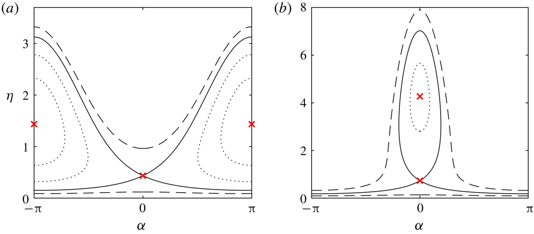
is a centre. The other two fixed points are unphysical, and are ignored. Figure 4(a) shows trajectories in the
 $(\unicode[STIX]{x1D6FC},\unicode[STIX]{x1D702})$
space. The heteroclinic orbits (solid lines) connecting the saddle points at
 $(2n\unicode[STIX]{x03C0},\unicode[STIX]{x1D6FD}_{-})$
and
 $(2(n+1)\unicode[STIX]{x03C0},\unicode[STIX]{x1D6FD}_{-})$
correspond to solitary waves with radial displacement
 $\unicode[STIX]{x1D6FD}_{-}$
in the far field. As expected, when
 $C=1-B/2$
, this value is unity. These solutions self-intersect, and are hence unphysical. The circular orbits (dotted lines) contained inside the heteroclinic orbits correspond to smooth periodic profiles, while the
 $2\unicode[STIX]{x03C0}$
periodic curves (dashed lines) correspond to self-intersecting periodic profiles.
Curves of constant
 $E$
in the
 $(\unicode[STIX]{x1D6FC},\unicode[STIX]{x1D702})$
plane. Both panels are for
 $B=1.25$
. (a) Has
 $C=-1$
, while (b) has
 $C=0.2$
. The critical points are labelled with crosses. The solid lines correspond to heteroclinic and homoclinic orbits, the dotted lines circular orbits and dashed lines
 $2\unicode[STIX]{x03C0}$
periodic curves.

Next, when
 $0<C<1/2B$
, we find that the fixed point
 $(2n\unicode[STIX]{x03C0},\unicode[STIX]{x1D6FD}_{-})$
is again a saddle point, and the fixed point
 $(2n\unicode[STIX]{x03C0},\unicode[STIX]{x1D6FD}_{+})$
is a centre. Figure 4(b) is an example of the
 $(\unicode[STIX]{x1D6FC},\unicode[STIX]{x1D702})$
space. The homoclinic orbit connecting the saddle point to itself corresponds to a smooth elevation solitary wave profile. The heteroclinic orbits connecting the saddle points are again self-intersecting solitary waves. Circular orbits correspond to smooth periodic profiles, and
 $2\unicode[STIX]{x03C0}$
periodic curves are self-intersecting periodic solutions. Finally, when
 $C>1/(2B)$
, there are no physical fixed points, and all trajectories are
 $2\unicode[STIX]{x03C0}$
periodic curves in the
 $(\unicode[STIX]{x1D6FC},\unicode[STIX]{x1D702})$
space, corresponding to self intersecting periodic profiles.
All of the solutions described above are one-dimensional profiles that satisfy (5.1) and
 $\unicode[STIX]{x1D702}\geqslant 0$
with
 $c=0$
. We integrate for values of
 $x$
along the curve of constant
 $E$
via the integral
 $$\begin{eqnarray}x=\int _{E=\text{const.}}\cot \unicode[STIX]{x1D6FC}\,\text{d}\unicode[STIX]{x1D702},\end{eqnarray}$$
to obtain the profile in the
 $(x,\unicode[STIX]{x1D702})$
space. This integral is evaluated numerically using the trapezoidal rule.
The solutions do not take into consideration any boundaries at
 $r=d$
and
 $r=D$
. It is of interest to note that we can interpret the profiles even if they intersect a boundary: the solutions can be seen as profiles which touch a boundary. We then consider the profile up to the point of contact, where the solution is reflected. This is demonstrated in figure 5, where two examples of a static profile (dashed curves) crossing a boundary (dotted curve) from above and below (a and b respectively) are interpreted this way. We only consider the portion of the profile satisfying
 $d\leqslant \unicode[STIX]{x1D702}\leqslant D$
. In (a), the dashed profile self-intersects, and is hence not physical without the inclusion of a boundary. The dashed profile of (b) is a static elevation solitary wave, and is a valid solution without the boundary. We note that these modified solutions disregard the complicated physical properties of contact angles (for example, see Batchelor Reference Batchelor1994, § 1.9). Despite this, the solutions are still of importance to consider, since many dynamic solution branches approach such static limiting configurations, as shown in § 6.
The dashed curves are profiles of static configurations. In (a), this static solution corresponds to a
 $2\unicode[STIX]{x03C0}$
periodic curve in the
 $(\unicode[STIX]{x1D6FC},\unicode[STIX]{x1D702})$
space, while in (b), it corresponds to a homoclinic orbit. The dotted curves we take as boundaries below (a) or above (b) the profile. The black curves show the modified solution, taken by reflecting the relevant part of the dashed profile.

In the next section, we discuss the results of the numerical procedure discussed in § 4 for non-static solutions, and how they relate to the static solutions discussed above.
6 Results
A thorough numerical investigation was performed by BP on the one-layer model for solitary waves. In this paper, we find new results for periodic and generalised solitary waves. We will repeat a discussion of the results of BP, since it will help to explain the solution space of the two-layer model, where there are many similarities. We differentiate between two distinct cases, when there does not exist a minimum in the dispersion curve (
 $B<B_{2}$
) and when there does exist a minimum (
 $B>B_{2}$
), describing the solution space in each instance. Below, we first consider
 $B<B_{2}$
.
6.1
 $B<B_{2}$

6.1.1 One layer
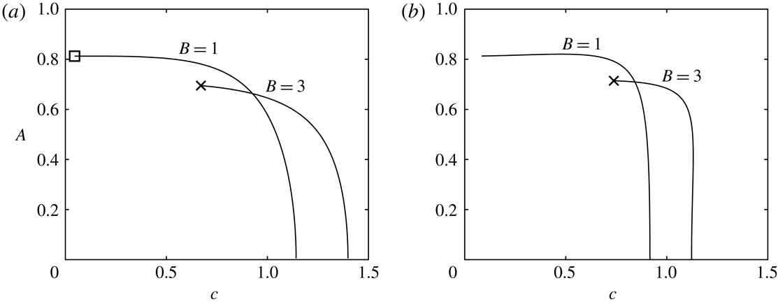
We begin by considering the solution space for the one-layer model. Using a linear solution (3.2) as an initial guess in the Newton iterations, we are able to use the numerical method described in § 4 to compute periodic solutions. Once on a solution branch, we can use the method of continuation to compute larger amplitude solutions. In figure 6(a), we show some solution branches for periodic waves for the one-layer model. These branches have the value
 $d=1.5/3.8$
, which is the value of
 $d$
used in the experiments of Bourdin et al. (Reference Bourdin, Bacri and Falcon2010). We computed branches for a variety of parameter values to determine the effect the parameters have on the solutions. Our findings are presented below.
Periodic solution branches with
 $\unicode[STIX]{x1D706}=\unicode[STIX]{x03C0}$
and
 $d=1.5/3.8$
. (a) Shows one-layer solution branches, while (b) is for two-layer solution branches with
 $D=2$
. In both cases, the
 $B=1$
branch terminates on a static profile which touches the bottom boundary
 $r=d$
. The
 $B=3$
branch for
 $\unicode[STIX]{x1D70C}=0$
overturns and ultimately forms a trapped bubble. The limiting configuration of the
 $B=3$
branch for
 $\unicode[STIX]{x1D70C}=1$
is unknown.

The solution branches terminate in a variety of ways. It can be the case that, given
 $B$
and
 $d$
are sufficiently small, the solution branch terminates on a smooth static profile. These static solutions were computed for
 $B=0$
by Vanden-Broeck et al. (Reference Vanden-Broeck, Miloh and Spivack1998). We cannot use the numerical scheme described in § 4 to compute the static profiles, since the method assumes the existence of a velocity field. However, one can continue along the solution branches up to small values of
 $c$
. We can then extrapolate to find an approximate value of the Bernoulli constant
 $C$
for
 $c=0$
. This allows us to find the set of static configurations in the
 $(\unicode[STIX]{x1D6FC},\unicode[STIX]{x1D702})$
space associated with the given Bernoulli constant, as described in § 5. Comparisons can then be made with the small
 $c$
profile and the static profile obtained by integrating along the curve of constant energy
 $E$
, where
 $E$
can be obtained by evaluating (5.2) at some mesh point on the interface of the small
 $c$
solution. Periodic smooth static profiles are orbits in the
 $(\unicode[STIX]{x1D6FC},\unicode[STIX]{x1D702})$
space. Figure 7(a) is a comparison between a one-layer solution with parameter values
 $B=0.05$
,
 $\unicode[STIX]{x1D706}=4$
,
 $d=0$
and
 $c=0.02$
, and the static profile obtained by integrating along the corresponding trajectory in the
 $(\unicode[STIX]{x1D6FC},\unicode[STIX]{x1D702})$
space (the
 $(\unicode[STIX]{x1D6FC},\unicode[STIX]{x1D702})$
space is shown in figure 7
b). The agreement between the two profiles obtained via different methods provides a check on our numerical method, and demonstrates that the solution branches can terminate on static profiles. These smooth static configurations only occur for small values of
 $B$
. For example, with the parameter values of the solution shown in figure 7, but with
 $B=0.1$
, it is found that the solution branch instead terminates on a static profile which touches the bottom boundary. This is described below.
(a) Shows a comparison between a one-layer solution found for
 $c=0.02$
(solid curve) and a smooth static profile (crosses). Only half a wavelength is shown. The solution has parameter values
 $d=0$
,
 $B=0.05$
and
 $\unicode[STIX]{x1D706}=4$
. (b) Shows the trajectories in the
 $(\unicode[STIX]{x1D6FC},\unicode[STIX]{x1D702})$
space. The dashed curve is the solution given by the crosses in (a). In (b), the cross is a saddle point and the circle a centre.

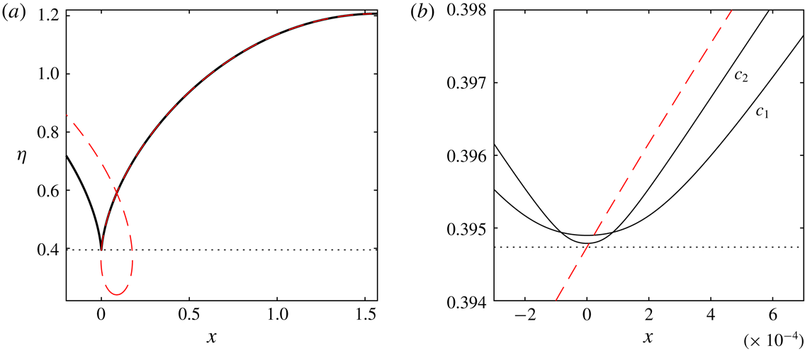
(a) Is a comparison between the solution corresponding to the square in figure 6(a) (given by the solid curve) and its corresponding
 $c=0$
solution (dashed curve). (b) Shows a blow up of the behaviour close to the point of contact for solutions with phase speeds
 $c=c_{1}=0.08$
and
 $c=c_{2}=0.05$
.

As mentioned in § 5, static profiles can be interpreted as solutions which touch a boundary. It is found that this configuration is a limiting case for many solution branches. Consider one-layer periodic solutions for varying values of
 $d$
. For a fixed
 $B$
, if
 $d$
is large enough, as we continue along a solution branch, the value of
 $c$
decreases as the solution forms a profile which gets very close to the boundary
 $r=d$
. A branch which terminates in such a manner is the
 $B=1$
branch from figure 6(a). The final solution computed along the branch (shown by the square in the figure) is a solution for
 $c=0.05$
. Figure 8(a) shows the profile of this solution. Computing a static profile with the same value of
 $C$
and
 $E$
results in a self-intersecting profile, shown by the dashed curve in the figure. The static profile agrees well with the
 $c=0.05$
solutions up to where the static solution intersects the boundary. Figure 8(b) shows a blow up of this region. The two solid curves are solutions with the phase speeds
 $c=c_{1}=0.08$
and
 $c=c_{2}=0.05$
. The image shows that as the speed is decreased further, the agreement between the curves and the static profile becomes stronger, and the thickness of the layer of fluid at the point of intersection continues to decrease. This provides numerical evidence that as
 $c\rightarrow 0$
, the dynamic profile approaches a static solution which touches the bottom boundary.
The final possible limiting configuration of one-layer periodic solution branches are profiles with a trapped bubble. Such branches occur for larger values of
 $B$
than the branches which terminate in static solutions. The
 $B=3$
branch of figure 6(a) is one such example, and the profile of the limiting configuration solution (corresponding to the cross in figure 6
a) is shown in figure 9. This limiting configuration has been found to occur for two-dimensional capillary and gravity–capillary waves, as found by Crapper (Reference Crapper1957), Kinnersley (Reference Kinnersley1976) and Hunter & Vanden-Broeck (Reference Hunter and Vanden-Broeck1983). Such solutions were also found for axisymmetric capillary waves (
 $B=0$
) by Vanden-Broeck et al. (Reference Vanden-Broeck, Miloh and Spivack1998). Continuing along the branch past the trapped bubble solutions, we find solutions with self-intersecting interfaces. Such solutions are not physically valid. It may be possible to extend the solution branch by allowing the pressure inside the bubble to vary, as was done by Vanden-Broeck & Keller (Reference Vanden-Broeck and Keller1980) for two-dimensional capillary waves. However, difficulties are experienced, since this introduces a discontinuity in (4.14), and hence in the derivatives of
 $r$
, which in turn would require a more sophisticated treatment in a finite difference scheme. This possible extension is beyond the scope of this paper. These intricate overturning solutions require a larger number of mesh points to retain accuracy. Consider the
 $B=3$
branch of figure 6(a). Fixing the phase speed to
 $c=0.7$
and allowing the amplitude to vary, table 1 shows the amplitude of the
 $c=0.7$
solution for different values of
 $M$
and
 $N$
. The table demonstrates the convergence of the numerical method for these extreme overhanging solutions.
Periodic solution corresponding to the cross in figure 6(a). (a) Shows one wavelength of the solution. (b) Is a blow up of the trapped bubble.

Values of the amplitude
 $A$
for the one-layer solution with parameter values
 $B=3$
,
 $d=1.5/3.8$
and
 $c=0.7$
for different mesh sizes. Issues with memory (the size of the Jacobian used in Newton’s method becomes very large) deny the possibility of computing a solution with
 $N=200$
and
 $M=300$
.

In § 3, we saw that when
 $B>1$
, all wavelengths are stabilised. This allows for the existence of pure solitary waves. Starting from small amplitude, as we increase
 $\unicode[STIX]{x1D706}$
, the waves form longer troughs and shorter crests. In the limit
 $\unicode[STIX]{x1D706}\rightarrow \infty$
, the solutions approach a solitary wave with a flat far field. These solitary wave branches bifurcate from the uniform stream at
 $c_{0}$
. Assuming
 $d=0$
, Rannacher & Engel (Reference Rannacher and Engel2006) obtained a KdV equation which approximates such solutions for small amplitude. Fully nonlinear computations of the solutions with arbitrary
 $d$
were done by BP. They found that, in agreement with the KdV equation, there exists critical values
 $B_{1}(d)$
and
 $B_{2}(d)$
such that when
 $B<B_{1}$
, the solitary waves are of elevation, while if
 $B_{1}<B<B_{2}$
, the solutions are depression waves. These waves get broader as the amplitude goes to zero, making it computationally impossible to compute the branches all the way to the bifurcation point.
As well as the solitary waves bifurcating from the uniform stream, BP found solitary waves solutions which bifurcate from finite amplitude. For
 $1<B<B_{1}$
, these branches are waves of depression. The amplitude from which these solution branches bifurcate decreases as
 $B$
increases up to
 $B_{1}$
. Meanwhile, for
 $B_{1}<B<2$
, the finite amplitude bifurcating branches are elevation solitary waves. The amplitude at which these branches bifurcates decreases as
 $B$
approaches
 $B_{1}$
from above. It would appear that the bifurcating amplitude of these two branches approaches zero as
 $B$
tends to
 $B_{1}$
. This is further supported by the analysis of Groves & Nilsson (Reference Groves and Nilsson2018), who for
 $d=0$
derived a cubic KdV equation (see (1.4)–(1.5) in their paper) for the model when
 $B$
is close to
 $B_{1}$
. The equation predicts both elevation and depression waves exist in this region, both of which bifurcate from zero amplitude. The numerical results of the present paper suggest that this is also true for non-zero values of
 $d$
, although difficulties in computing solution branches up to the point of bifurcation due to wave broadening deny conclusive numerical evidence.
The existence of the finite amplitude bifurcating pure solitary waves is in stark contrast with the gravity–capillary problem, where such solutions have not been observed. Continuing the branches beyond the bifurcation point into large amplitudes, BP found that depression waves terminate in either static profiles which touch the bottom boundary, or overturning waves with a trapped bubble, while elevation solitary wave branches terminate in smooth static configurations. This is similar to the periodic limiting configurations. The only difference occurs for the nonlinearly bifurcating
 $B=2$
solitary wave branch, which was found to increase indefinitely in amplitude. We can gain some insight as to why this is the case by considering the static configurations. Smooth static elevation solitary waves correspond to the homoclinic orbit connecting the saddle point to itself in figure 4(a). Taking
 $C=1-B/2$
, there does not exist such orbits when
 $C\leqslant 0$
(i.e.
 $B\geqslant 2$
). Therefore, there is no limiting static configuration for the
 $B=2$
elevation branch, offering a possible explanation as to why the
 $B=2$
branch has this unique behaviour, and why elevation branches do not exist for larger values of
 $B$
.
6.1.2 Two layers
Next, we shall discuss the solution space for the two-layer model when the dispersion relation is monotonic increasing. Again, starting from linear solutions, we can use the method of continuation to compute periodic solution branches. Some periodic solution branches are shown in figure 6(b). These branches have the same parameter values as the one-layer periodic branches of figure 6(a), except for a density ratio of unity between the two fluids (since it is the two-layer model), and an additional outer boundary at
 $r=D$
, where
 $D=2$
. The
 $B=1$
branch, as with the one-layer
 $B=1$
branch, terminates on a static profile which touches the boundary
 $r=d$
. Decreasing the value of
 $D$
, one finds the solution branches can also terminate on static profiles which touch the upper boundary. For example, for the
 $B=1$
branch discussed above, taking the same parameter values but changing
 $D$
to
 $D=1.3$
results in such a limiting configuration.
Periodic solution corresponding to the cross in figure 6(b). Two wavelengths are shown. Streamlines in the ferrofluid are the black curves, while streamlines in the second fluid are the dashed curves. Not all streamlines have been plotted. This is the largest amplitude solution computed on this solution branch. The branch could not be computed further due to difficulties with overturning.

Next, consider the
 $B=3$
branch. Due to the similarities between the one-layer and two-layer models for the
 $B=1$
model, one may expect this solution branch to form overturning solutions, and eventually form a trapped bubble. Unfortunately, as mentioned earlier, the numerical method described in § 4 cannot compute overturning solutions for the two-layer model. This is due to the interpolation procedure for values on the interface being performed in the
 $x$
variable, for which overturning solutions are not single valued. One may be tempted to instead interpolate in the
 $r$
variable, for which these solutions are single valued. However, the code is extremely sensitive to this method and fails to converge. We have computed the
 $B=3$
branch from figure 6(b) as far as computationally possible with the method. The profile of this solution is shown in figure 10. We believe the solution will overturn as one continues along the branch. However, a new numerical treatment of the problem will be required to investigate these solutions. Overturning two-dimensional gravity–capillary internal waves have been found in the recent numerical and analytical investigations of Akers et al. (Reference Akers, Ambrose, Pond and Wright2016).
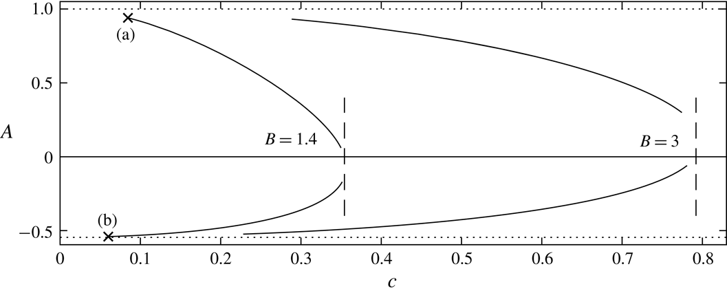
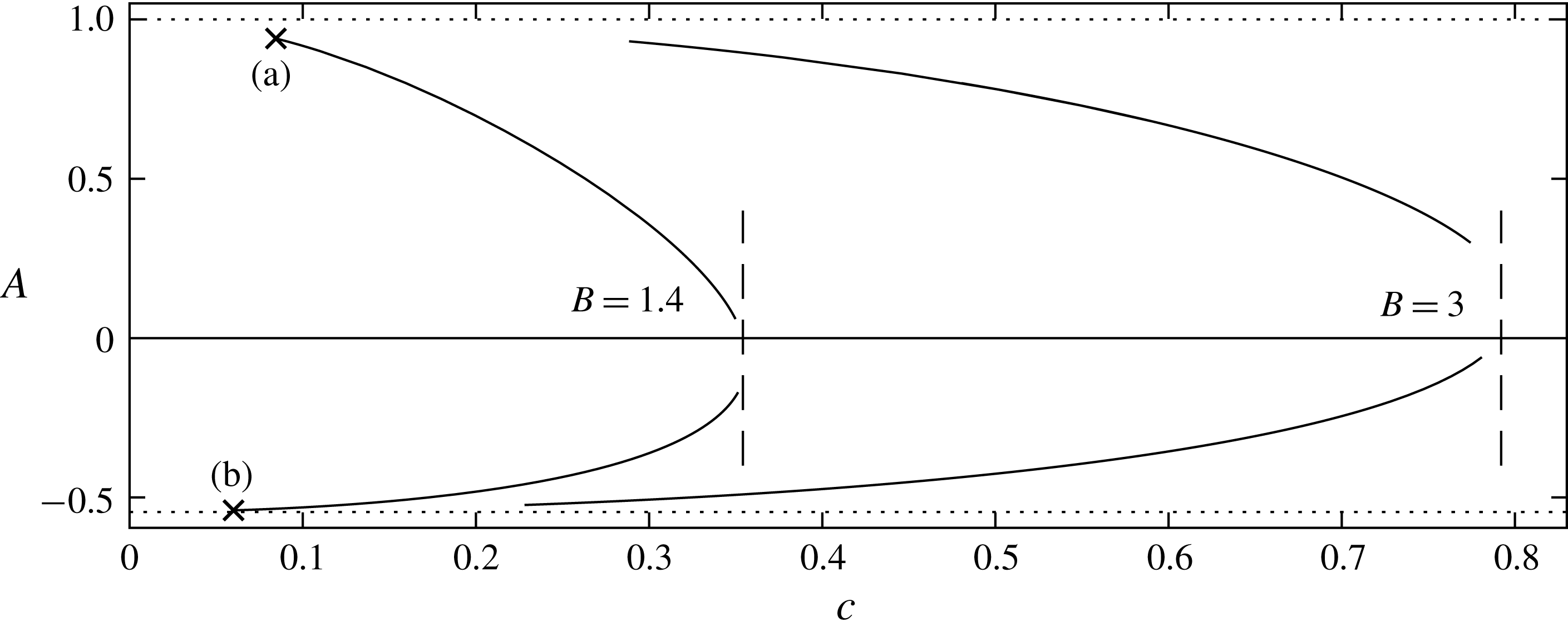
Two-layer pure solitary wave branches with
 $d=1.5/3.3$
and
 $D=2$
for
 $B=1.4$
and
 $B=3$
. The dashed curves show the value of
 $c_{0}$
for the two choices of
 $B$
, while the dotted curves correspond to the maximum possible value of the amplitude, where the profile touches a boundary. The points (a)–(b) refer to the solutions shown in figure 12.
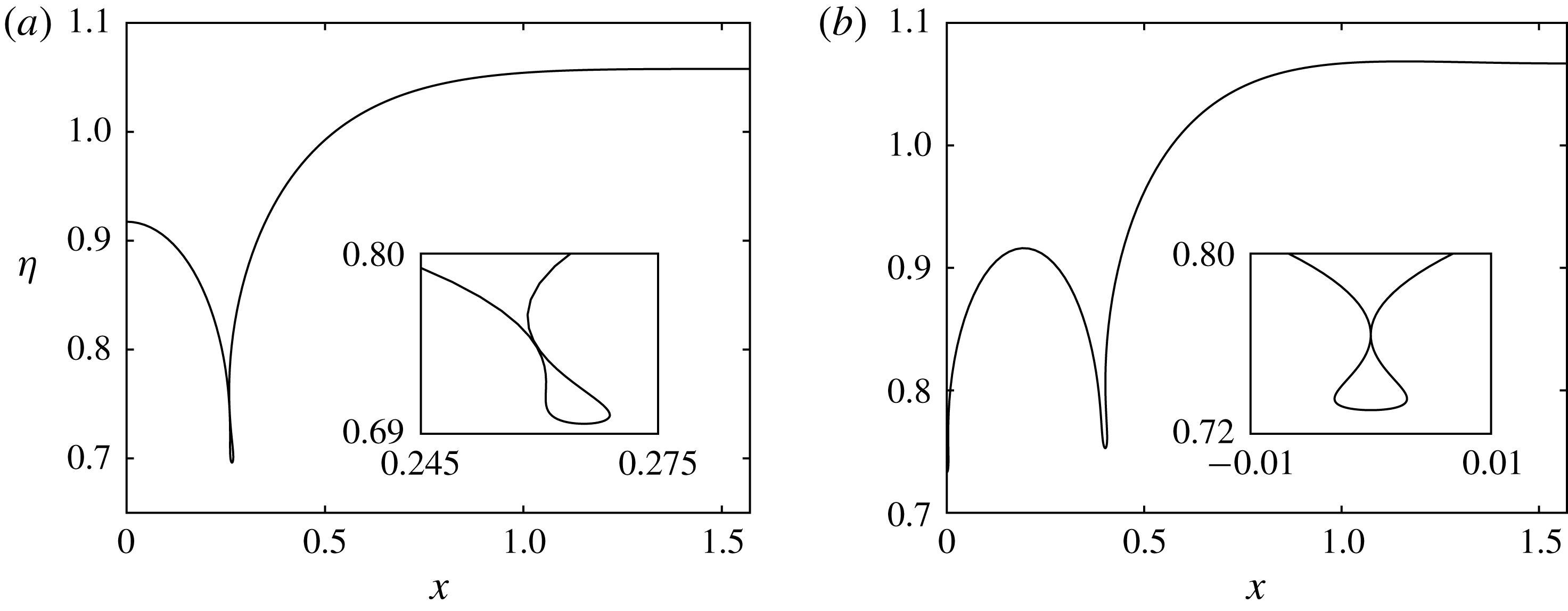
Profiles corresponding to the points (a) and (b) in figure 11. They approach static profiles which touch
 $r=D$
and
 $r=d$
respectively. The dotted curves are static profiles which the solutions approach as
 $c\rightarrow 0$
.

For
 $B>1$
, we again expect to see pure solitary waves. Some solution branches for
 $d=1.5/3.3$
and
 $D=2$
are shown in figure 11. It can be seen that for
 $B=1.4$
, the elevation branch bifurcates from zero amplitude, while the depression branch bifurcates from non-zero amplitude. The roles are reversed for
 $B=3$
, implying
 $B_{1}\in (1.4,3)$
for the given values of
 $d$
and
 $D$
. Due to the existence of the upper boundary
 $r=D$
, the elevation branches can now terminate on static profiles which touch the boundary. This is shown in figure 12(a), where an elevation solitary wave for
 $c=0.1$
is shown to be in good agreement with a static profile that crosses
 $r=2$
. This new limiting configuration means that, unlike for the one-layer model, there now exists pure elevation solitary waves (bifurcating from finite amplitude) for values of
 $B>2$
. One does not have to consider the case when there is no upper boundary for two-layer pure solitary wave solutions, since BP showed that when
 $D\rightarrow \infty$
, there exists a minimum in the dispersion curve for
 $B>1$
, removing the possibility of pure solitary waves (it can be seen from (3.10)–(3.12) that
 $B_{2}\rightarrow 1$
as
 $D\rightarrow \infty$
).
A description of the solution space when there exists a minimum is presented in the following section.
6.2
$B>B_{2}$

As stated previously, if
 $B>B_{2}$
, then a minimum occurs in the dispersion relation. We will discuss the results for the one-layer and two-layer models simultaneously, since the solution spaces in this regime are qualitatively similar. The only difference occurs for overhanging solutions, where our inability to compute overhanging solutions for the two-layer model means the limiting configurations of some two-layer solution branches remain unknown. This is discussed below.
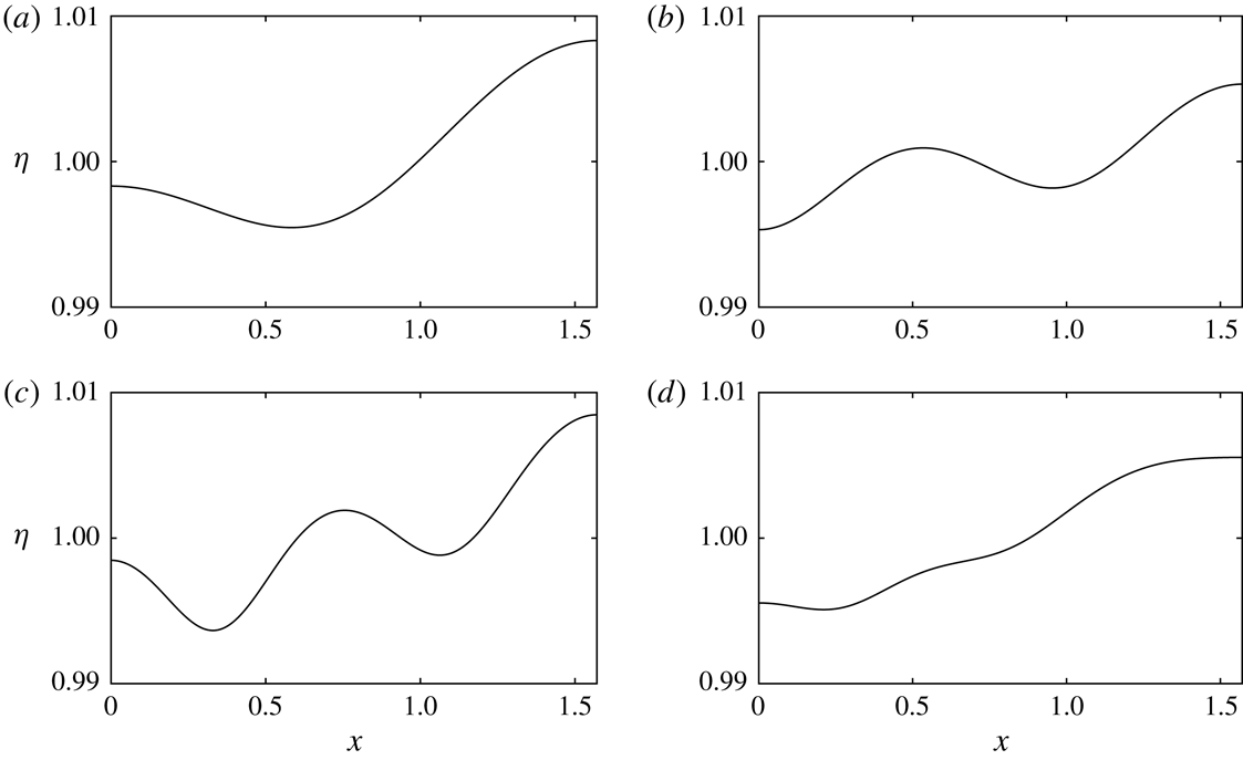
One-layer solutions exhibiting higher mode resonance for
 $\unicode[STIX]{x1D706}=\unicode[STIX]{x03C0}$
and
 $d=0$
. Only half a wavelength is shown. The values of
 $B$
are
 $B=16.4$
,
 $B=21.7$
,
 $B=27.2$
and
 $B=32.8$
while the values of
 $n$
in (3.5) are
 $n=2,3,4,5$
for (a), (b), (c) and (d) respectively.

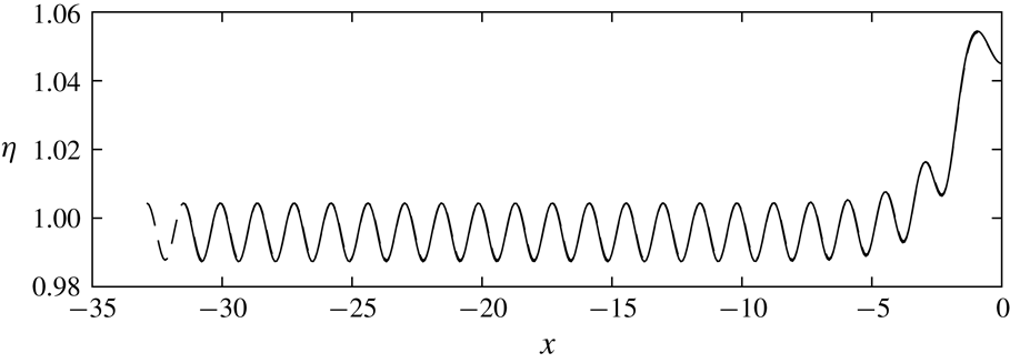
Two one-layer long wave solutions with parameter values
 $B=13$
,
 $d=0$
,
 $c=12.5$
and
 $\unicode[STIX]{x1D702}(0)=1.045$
, and wavelengths
 $\unicode[STIX]{x1D706}=65.8$
(solid curve) and
 $\unicode[STIX]{x1D706}=71.1$
(dashed curve). It can be seen that the two profiles almost perfectly overlap, where the longer solution has an additional periodic wave in the tail.

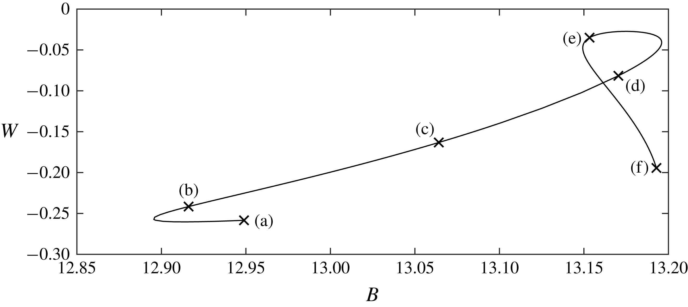
Generalised solitary wave branch for
 $\unicode[STIX]{x1D702}(0)=1.045$
and
 $\unicode[STIX]{x1D706}=63$
. Some profiles corresponding to points on the branch are shown in figure 17.

When there is a minimum in the dispersion curve, we see periodic solutions exhibiting higher mode resonance, as described by (3.5). These solutions exist for integer values of
 $n>1$
when
 $c(k)=c(nk)$
, where
 $c$
is given by (3.3). Fixing a value of
 $k$
and
 $n$
, we can find a value of
 $B$
such that this equality is satisfied. Using these parameter values, we are able to compute solutions with Wilton ripples, as shown in figure 13 for
 $n=2,3,4,5$
. These solutions are for the one-layer model. One can continue these branches of solutions into highly nonlinear regimes by further increase of the amplitude. They form interesting profiles, where the depression of each ripple begins to overturn (see figure 14). They terminate once one of the overhanging structures forms a trapped bubble. These results can be repeated for the two-layer problem, although as before we are unable to extend solution branches beyond the point of overturning.
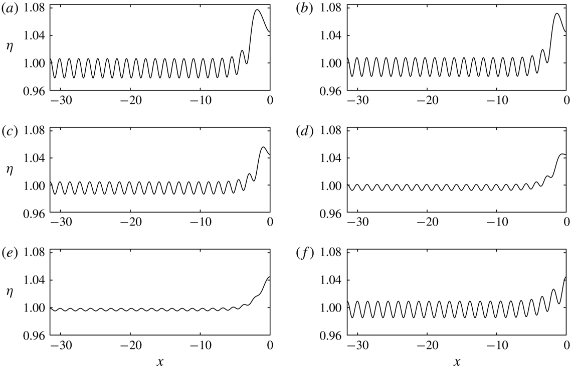
Generalised solitary waves corresponding to points (a)–(f) in figure 16. Only half a wavelength is shown.


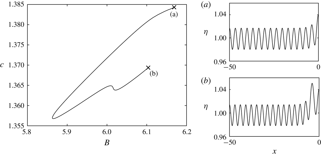
Two-layer generalised solitary wave branch for
 $d=1.5/3.3$
,
 $D=3$
,
 $\unicode[STIX]{x1D702}(0)=1.04$
and
 $\unicode[STIX]{x1D706}=100$
. Two profiles corresponding to points (a) and (b) are shown. Only half the solution is shown in (a) and (b).

Increasing the wavelength of periodic solutions when
 $c(k)$
has a minimum results in a larger central peak or trough, and a train of smaller amplitude waves in the far field. Denote the wavelength of the far-field waves as
 $\hat{\unicode[STIX]{x1D706}}$
. Increasing the wavelength of the solution by
 $\hat{\unicode[STIX]{x1D706}}$
results in two almost overlapping solutions, where the longer wave has one additional linear wave in the far-field. This is demonstrated in figure 15. One can easily add more waves to the far field, limited only by computational storage. These solutions are finite wavelength approximations of generalised solitary waves. As one would expect,
 $\hat{\unicode[STIX]{x1D706}}$
is found to be the finite valued wavelength which gives
 $c(\hat{\unicode[STIX]{x1D706}})=c_{0}$
. These waves were computed by Vanden-Broeck (Reference Vanden-Broeck1991) and Champneys et al. (Reference Champneys, Vanden-Broeck and Lord2002) for gravity–capillary waves. We present a generalised solitary wave solution branch for the one-layer problem in figure 16, and the corresponding profiles in figure 17. We fixed
 $\unicode[STIX]{x1D702}(x=0)=1.045$
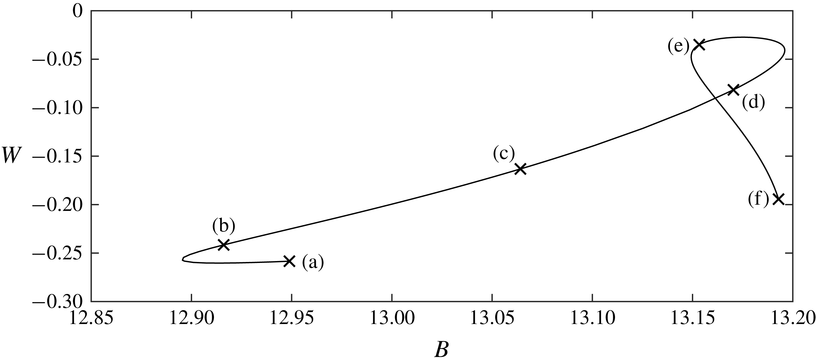
, and vary the speed of the wave. Due to the imposed symmetry, and since these solutions are finite wavelength approximations of generalised solitary waves, the far-field wave train ends in either a peak or a trough. We can see in figure 17 (by looking at the leftmost point of the profile) that in this case it is a peak. As with gravity–capillary waves, the branches start and end on solutions with larger amplitude far-field waves. For solutions in between the ends of the branch, the amplitude of the waves in the far field is smaller (see figure 17). No solutions with a flat far field were found. This is shown numerically in figure 18, where the reciprocal of the radius of curvature of the free surface, given by
 $$\begin{eqnarray}W=\frac{\unicode[STIX]{x1D702}_{xx}}{(1+\unicode[STIX]{x1D702}_{x}^{2})^{1/2}},\end{eqnarray}$$
is shown to be strictly negative when evaluated at the furthest mesh point in the far field for all solutions on the branch. The KdV equation of Rannacher & Engel (Reference Rannacher and Engel2006) predicts pure elevation solitary waves in this region, and hence fails to accurately describe fully nonlinear solutions when
 $B>B_{2}$
. Generalised solitary wave branches with the same behaviour were found for the two-layer problem, where one such branch is presented in figure 19.
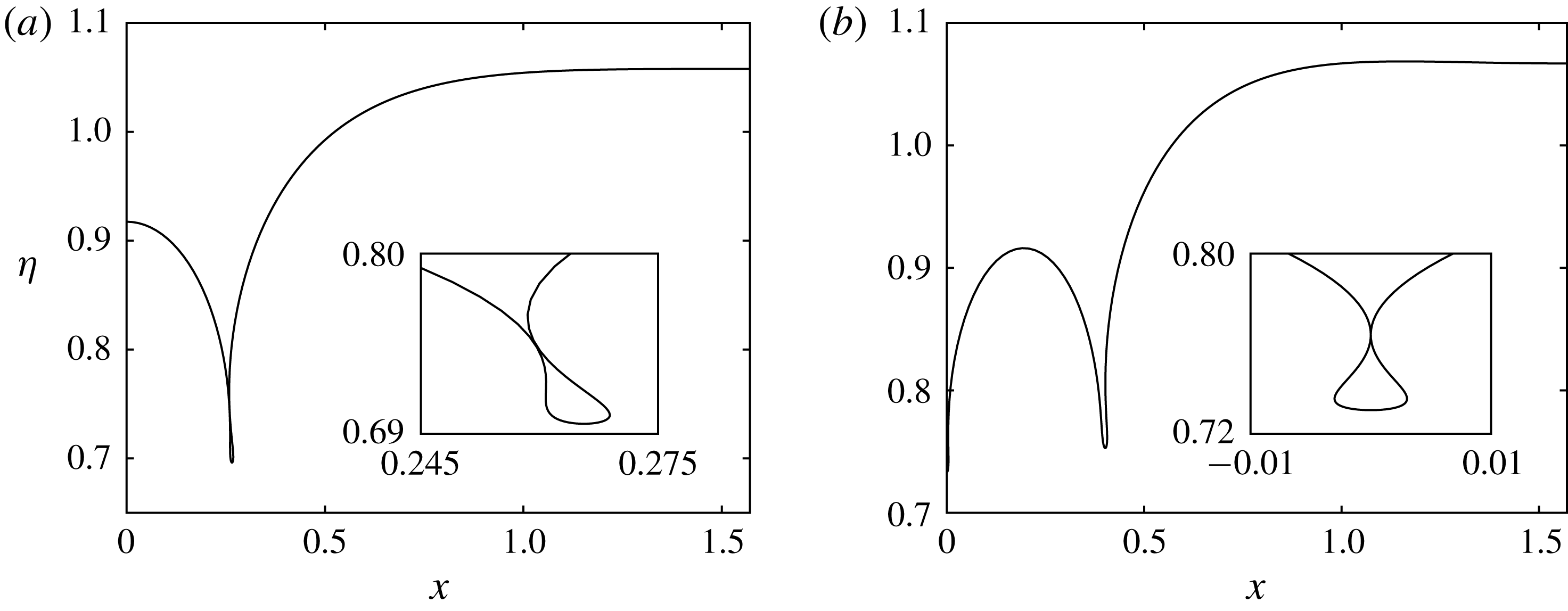
One-layer solitary wave packets for
 $d=1.5/3.3$
,
 $B=20$
. (a) Is the limiting configuration of the depression branch and (b) the furthest point computed on the elevation branch. The inset of (a) shows the trapped bubble.

Although there do not exist pure solitary waves bifurcating from zero amplitude at
 $c_{0}$
, there do exist branches of solitary wave packets bifurcating from a linear wave train of wavenumber
 $k_{m}$
at
 $c_{m}$
. Use of the chain rule shows that at the minimum of the dispersion relation, the group velocity of linear waves is equal to the phase velocity. This allows the existence of solitary wave packets (Akylas Reference Akylas1993), in particular one depression branch and one elevation branch. At small amplitudes, these waves are described by a nonlinear Schrödinger equation, as derived for the one-layer model (assuming
 $d=0$
) by Groves & Nilsson (Reference Groves and Nilsson2018). Fully nonlinear solutions for the one-layer problem were computed numerically by BP. They found that as one increases the amplitude along the depression branch, the solutions begin to overturn, forming a trapped bubble. Repeating the numerical scheme for variable parameter values, we found the overturned bubble does not have to occur at the point of symmetry, but can also appear at some other point in the profile, as seen in figure 20(a). For no parameter values tested did the solution branches approach a static configuration. This is in agreement with § 5, where the range of static solutions found did not include solitary waves with decaying oscillating tails.
Two-layer solitary wave packets with amplitude
 $A=-0.1$
, for
 $d=1.5/3.3$
,
 $B=8.3$
and
 $D=2$
(dotted curve),
 $D=4$
(dashed curve) and
 $D=8$
(solid curve). Only one half of the profile is shown. The dashed and solid curves almost overlap.

BP conjecture that the elevation branches overturn and form trapped bubbles as well, although they note care must be taken since this conjecture was mistakenly made by Vanden-Broeck & Dias (Reference Vanden-Broeck and Dias1992) for two-dimensional gravity–capillary elevation solitary wave packets. The more accurate computations of Dias, Menace & Vanden-Broeck (Reference Dias, Menace and Vanden-Broeck1996) demonstrated that these solution branches actually turn around and form many loops in the
 $(c,\unicode[STIX]{x1D702})$
space. Figure 20(b) shows a solution from the elevation branch, computed as far along the branch as possible. Both solutions where computed with
 $N=30$
and
 $M=900$
. These solutions also exist for the two-layer model. This is expected, since the same phenomenon occurs for two-dimensional internal gravity–capillary waves (Laget & Dias Reference Laget and Dias1997). In figure 21, we show a two-layer depression solitary wave packet, with varying values of
 $D$
. As
 $D$
gets larger, the variation in the profiles becomes small. It follows that one could approximate the case of a surrounding fluid of infinite radius (
 $D\rightarrow \infty$
) by taking a suitably large value of
 $D$
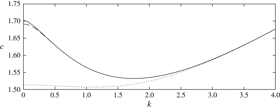
. This is further confirmed by considering the dispersion relation (3.3) for various values of
 $D$
, as shown in figure 22. It can be seen that the dispersion relations for
 $D=8$
and
 $D\rightarrow \infty$
are very similar, the largest difference occurring at
 $k\rightarrow 0$
(the long wave speed).
Two-layer dispersion relation, given by (3.3), with
 $d=1.5/3.3$
,
 $B=8.3$
and
 $D=2$
(dotted curve),
 $D=8$
(dashed curve) and
 $D\rightarrow \infty$
(solid curve).

There are difficulties with comparing the two-layer numerical results of this paper with the experimental data of Bourdin et al. (Reference Bourdin, Bacri and Falcon2010), as was discussed in BP. For completeness, we highlight the key points here. Bourdin et al. coated a copper wire of radius 1.5 mm with a ferrofluid jet of radius 3.8 mm when creating periodic waves, and 3.3 mm when creating solitary waves. The ferrofluid was surrounded in freeon of almost equal density, and the whole system was contained in a cuboid container with a
 $40~\text{mm}\times 40~\text{mm}$
side and 30 mm length. The fact that axisymmetric profiles were witnessed in a cuboid container implies that the effects of the container were negligible. Hence, to compare our model with these experimental results, we wish to consider the case of a surrounding fluid of infinite radius. As shown above, this can be approximated by considering a large value of
 $D$
. Bourdin et al. observed pure solitary waves: a depression wave for magnetic Bond number
 $B=8.1$
and a wave of elevation for
 $B=10.5$
. As noted by BP, and confirmed by the results in this paper, one would expect to see solitary wave packets or generalised solitary waves for such parameter values, due to the occurrence of minimum in the dispersion curve. This is at odds with the pure elevation and depression solitary waves witnessed by Bourdin et al. However, we suspect the inclusion of the effects of the second fluid are not negligible. Evidence for this was given by BP, who showed that the agreement between the experimental and theoretical dispersion curve improved when taking the second fluid to have equal as opposed to negligible density. It would be of interest to see further experimental results on the problem.
7 Conclusion
In conclusion, we have presented a numerical model capable of finding stable travelling wave solutions on a ferrofluid jet, where the surrounding fluid is assumed to be of zero density or equal density to that of the ferrofluid. The results from the classical problem of two-dimensional gravity–capillary waves have helped predict the behaviour of the solution space for various parameter values. The importance of the existence of a minimum in the linear dispersion relation has been demonstrated, and periodic, solitary and generalised solitary waves have been found for both models. The stability of the solutions is as of yet unknown, and would require a time dependent numerical scheme to find out, as done by Guyenne & Părău (Reference Guyenne and Părău2016) for pure solitary waves on the one-layer model. As well as time dependent models, it would be interesting to see if symmetry breaking bifurcations can be found with the numerical scheme described in this paper (by removing the imposed symmetry condition), as has been found by Gao, Wang & Vanden-Broeck (Reference Gao, Wang and Vanden-Broeck2017) for gravity–capillary waves.
Acknowledgements
A.D. was supported under grant EP/M507970/1. J.-M.V.-B. was supported in part under grant EP/N018559/1. The authors would like to thank the ESI (Erwin Schrödinger Institute) for financial support during the ‘Nonlinear water waves – an interdisciplinary interface’ workshop.