Candidate quality differences can produce significant changes in the nature of political competition. The equilibrium properties of spatial competition between two candidates who differ in quality have been analyzed theoretically and the aim of this paper is to test them using experimental data. The main properties are that higher-quality candidates tend to choose more moderate locations and that uncertainty about the median voter helps lower-quality candidates. We find that all the main qualitative properties of this equilibrium are clearly observed in the data obtained from laboratory experiments. Moreover, the results are robust across subject pools and experimental context.
Candidate quality is widely considered to be a critical variable in electoral competition.1
For example, most studies of the incumbency advantage in congressional elections identify challenger quality as a critical factor. See, e.g., Jacobson and Kernell (1981), Krasno (1994), and Squire (1992). Incumbency itself can also be viewed as an indicator of quality.
It affects the decisions of politicians to run for office, campaign fund-raising and advertising, voter behavior, election outcomes, and, ultimately, policy outcomes. While direct measurement of candidate quality is often elusive, few doubt its importance in electoral politics. Quality differences between two candidates can arise for many reasons, including charisma, officeholding experience, incumbency, advertising, scandal, and other nonpolicy dimensions that can affect the relative attractiveness of two candidates. Political scientists have demonstrated over several decades of careful empirical research the importance of these and other image factors, or the “valence dimension,” as it is referred to in numerous articles and books.
2 See, e.g., Kiewiet (1983), Kiewiet and Zheng (1993), and Stokes (1963).
It is obvious that, all else constant, high-quality candidates will fare better than low-quality candidates. What is less obvious, but equally important, is that quality differences produce significant changes in the nature of political competition. Recent papers by Ansolobehere and Snyder (2000), Aragones and Palfrey (2002), and Groseclose (2001) report a number of theoretical results about the equilibrium properties of spatial competition between two candidates who differ in quality.3
There are also some earlier theoretical papers that studied other kinds of asymmetry, such as incumbency and partisanship, e.g., Adams (1999), Bernhardt and Ingberman (1985), Ingberman (1992), and Londregan and Romer (1993).
The results are striking and suggest that the indirect equilibrium effects of candidate quality differentials may be even more important in determining candidate policies and election outcomes than the direct effects of producing more votes for one candidate than the other.
4 Using a different approach, Banks and Kiewiet (1989) show that candidate quality differentials can have important and surprising equilibrium effects on the entry of challengers in congressional elections. Dasgupta and Williams (2002) study information aggregation through polls in a principal-agent model with incomplete voter information about candidate quality. They report experimental results supporting their rational expectations hypothesis.
The main insight about spatial competition if the candidates differ in quality (or along some other valence dimension) is that the better candidate has an incentive to copy the policies of the inferior candidate, or at least move in that direction, while the disadvantaged candidate has the opposite incentive, to move away from the advantaged candidate. Theoretically, the advantaged candidate will win all the votes if the two candidates choose sufficiently similar policies. Thus, in the standard Downsian model where candidates are purely office-motivated, the disadvantaged candidate must mix in order not to be predictable. However, in order for mixing to be an equilibrium strategy for the disadvantaged candidate, the advantaged candidate also must be mixing.5
An equilibrium in mixed strategies is guaranteed to exist (Aragones and Palfrey 2002), and has intuitive properties. A pure strategy equilibrium may exist if candidates obtain utility from winning policies as well as from holding office, under certain conditions. Groseclose (2001) studies the properties of stable pure strategy equilibria, under the maintained assumption that they exist, but does characterize conditions for existence. He presents an example suggesting that existence is especially problematic for small to intermediate values of the quality advantage and if officeholding is the primary motivation of candidates. The properties of pure strategy equilibria are similar to those of mixed equilibria.
This implies the first of three key properties of equilibrium in these models: The equilibrium makes statistical predictions, not point predictions. If both candidates have complete information and symmetric beliefs about voters, then the equilibrium is generally in mixed strategies. If candidates have private information with continuous types, then this mixed equilibrium can be “purified.” That is, there will exist an equilibrium in pure strategies, where the equilibrium locations of candidates will vary with this private information. Moreover, both the pure and the mixed strategies produce distributions of location decisions that share similar statistical properties (Aragones and Palfrey 2004).
The second key property is that the distribution of location decisions of the two candidates will be different from each other, and the differences are systematic. We call this the quality divergence hypothesis. The main difference between the two candidate locations is that the distribution of locations of the better candidate is concentrated in the center of the policy space (i.e., the expected location of the median voter), while the location of the disadvantaged candidate tends toward the extremes. That is, better candidates tend to choose more moderate locations. Groseclose (2001) notes that this is consistent with two regularities that have been identified in empirical studies of congressional elections. One is the lack of support for the marginality hypothesis, documented in Fiorina (1973). That is, Fiorina finds that incumbents who are in marginal districts tend to moderate less than incumbents from safe districts. This is clearly consistent with the quality divergence hypothesis. Second, a recent paper by Ansolobehere, Snyder, and Stewart (2001) compares the spatial locations of three categories of candidates: (1) incumbents seeking reelection, (2) candidates for open seats, and (3) challengers running against an incumbent. They find that incumbents are the most moderate, followed by open seat candidates, and that challengers adopt the most extreme positions. To the extent that quality correlates across these three categories as expected, then this provides further corroboration of the quality divergence hypothesis.
The third property is that the two candidates' equilibrium distributions of locations varies systematically with the degree of uncertainty about the median voter. Uncertainty helps the disadvantaged candidate, who chooses more moderate locations as a strategic response to greater uncertainty. This implies that the quality divergence effect is weakest when there is a lot of uncertainty or if the electorate is highly polarized, and the effect is strongest when there is little uncertainty or a high degree of consensus in the electorate. We call this the polarization hypothesis.
Because the nature of equilibrium is very subtle in these asymmetric spatial competition games, and because the equilibrium (with complete information) is mixed, one cannot help but be skeptical about whether the features of the theoretical equilibrium might actually occur in practice. While the evidence put forth by Groseclose (2001) is consistent with the quality divergence hypothesis, that evidence could be explained by other theories. For example, the correlation between incumbency (i.e., electoral success) and moderation is also consistent with the standard Downsian model or the more general models by Calvert (1985) and Wittman (1983), which include policy motivations. Thus, the evidence is suggestive that the theory may be on the right track but does not provide a conclusive test of the model. Unfortunately, the kind of field data one would need to test these predictions is simply not available, due to the difficulty of obtaining reliable and accurate measurement of the “quality” variable, the degree of uncertainty or polarization in the electorate, and the location of candidates, and because the statistical nature of predictions would require a large number of observations. We believe that direct testing of the theory is needed.
With this in mind, we designed and conducted laboratory experiments to test directly both the quality divergence hypothesis and the polarization hypothesis. By doing so, we hope to find out if the basic predictions of the theory are accurate and, if not, what sort of modification of the theory might be required. This paper reports and analyzes the data from those experiments.
There are three main findings. First, all of the qualitative predictions from the equilibrium theory were clearly observed in the data. Both the quality divergence hypothesis and the polarization hypothesis are strongly supported by the data. Location decisions were statistical, the advantaged candidates located more centrally on average, and all of the comparative static predictions of changes in the distribution of voters were observed. In particular, when the distribution of voters was more polarized, there was less divergence. Second, the results are robust across subject pools and experimental contexts. We used two subject pools, one from California, USA, and the second from Barcelona, Spain. While the subjects were university students in both cases, they were from much different backgrounds both culturally and politically. The results are virtually identical in the two datasets. Most of the experimental sessions were conducted in a context-free setting, as is standard practice in controlled game theory experiments. In addition, we conducted one session where subjects played the role of vote maximizing candidates in a sequence of two-candidate elections. In each election, they selected policies. The number of votes they received was a (commonly known) function of their policy and the policy of the opposing candidate. This function was constructed to be the same as the “point” payoffs in the abstract setting. Subjects earned money in direct proportion to the number of votes they received.6
Alternatively, we could have explained these payoffs as the probability of winning, with identical equilibrium predictions. We opted for the vote maximization model because it is simpler to explain.
Third, while the main hypothesis were clearly supported, the exact distribution of location choices was somewhat different from the quantitative predictions of the theory in systematic and surprising ways. There were two noteworthy differences: (a) Both candidates showed a bias toward centrist locations, relative to the theoretical predictions; and (b) the disadvantaged candidate's location distribution was less responsive to changes in uncertainty than predicted by the theory.
In order to account for these anomalies, we consider an extension of Nash equilibrium theory that allows for a limited amount of bounded rationality. This approach, called Quantal Response Equilibrium (QRE; McKelvey and Palfrey 1995, 1996), is based on two principles. The first principle is that players of any game respond continuously, but imperfectly, to the incentive structure of the game. While they do not optimize perfectly, they will choose on average better strategies more often than worse strategies. The second principle is that players are aware that other players are also imperfect and take this into account when choosing their actions.
This boundedly rational version of Nash equilibrium often leads to surprising and unintuitive predictions about behavior in games and provides a statistical model for data analysis. Recently this model has been used in a number of political science applications, spanning empirical studies, experimental studies, and theoretical modeling. For example, Signorino (1999) has applied it in a model of international conflict, Guarnaschelli, McKelvey, and Palfrey (2000) apply it to jury decision making, and McKelvey and Patty (2002) use it as a basis for a theoretical model of candidate competition with probabilistic voting. To analyze our data using this approach, we fit the data to the Logit version of QRE. We find that the simplest one-parameter version of that model provides an excellent fit to the data and accounts for the two unexpected findings.
THE MODEL
We begin with a synopsis of the model and basic results of Aragones and Palfrey (2002). The reader is referred to that paper for details. The policy space is one-dimensional and consists of the set of n>1 equally spaced points on the [0, 1] interval.7
This is just a discrete version of the standard spatial model.
There are two candidates,
A and
D, who are referred to as the advantaged candidate and the disadvantaged candidate, respectively. Each candidate's objective is to maximize the probability of winning the election.
8 This is equivalent to a model of vote maximizing candidates facing a known distribution of voters.
Each voter has a utility function, with two components, a
policy component and a candidate
image component. The policy component is characterized by an ideal point in the policy space with utility of alternatives in the policy space a strictly decreasing function of the distance between the ideal point and the location of the policy, symmetric around the ideal point. We assume that there exists a unique median location. Candidates do not know the exact location of the median voter but share a common prior belief about it. This commonly shared belief is represented by a uniform distribution. The image component of a voter's utility is captured by a positive constant that is added to the utility each voter gets if
A wins the election.
9 The constant could be different for different voters. For simplicity, we have assumed that it is the same.
The image component is assumed to be small, relative to the policy component of utility.
The game takes place in two stages. In the first stage, candidates simultaneously choose positions in the policy space. In the second stage, each voter votes for the candidate whose victory would yield the higher utility.
A pure strategy equilibrium is a pair of candidate locations such that both candidates are maximizing the probability of winning given the choices of the other candidate. A mixed strategy equilibrium is a pair of probability distributions over locations such that both candidates are maximizing the probability of winning given the mixed strategy of the other candidate.
There are five main results, each of which we state without proof.10
There are some additional technical assumptions. The reader is referred to Aragones and Palfrey (2002) for formal statements and proofs of these results.
Result 1: There does not exist a pure strategy equilibrium.11
Versions of this proposition can be found in Berger, Munger, and Potthoff (2000) and Groseclose (2001). Ansolobehere and Snyder (2000) contains some related results.
Result 2: There exists an essentially unique equilibrium in mixed strategies.
Result 3: The distribution of D's equilibrium strategy is U-shaped (with a local minimum at the expected median).
Result 4: The distribution of A's equilibrium strategy is single-peaked (at the expected median).
Result 5: The probability that A wins is higher than the probability that D wins.
Summarizing, the main results are that there exists an essentially unique equilibrium in symmetric mixed strategies with no gaps. In this equilibrium, A is the more likely candidate to win. That is, A's quality advantage leads to an electoral advantage. The supports of the equilibrium mixed strategies are the same, but otherwise the two distributions of the two candidates' are much different. The better candidate is more likely to locate in the center of the policy space than at the extremes, while the opposite is true for the lower-quality candidate. The latter property follows from results 3 and 4, and we call it the quality divergence effect.
THE EQUILIBRIUM EFFECTS OF UNCERTAINTY
This paper conducts an experiment to test a number of the predictions of the theoretical model. We use a variation on this model that can be solved explicitly for arbitrary distributions of the median voter. This is important because the equilibrium strategies of the candidates are sensitive to the distribution and vary in systematic ways with the distribution. This variation, in which candidates can choose one of only three locations (left, center, right), also has the virtue of being quite simple and intuitive to explain to subjects.12
This method is also used in the Dasgupta and Williams (2002) experiment.
This is important in the laboratory context, since we use naive subjects who have had no real experience in candidate location games.
13 A completely general solution to this three-location model is given in Aragones and Palfrey (2002). We present only a synopsis of the derivation here.
Denote the three possible locations, L, C, and R, for left, center, and right, respectively, where L<C<R. The probability that the median voter is located at ideal point L is denoted α; similarly the probability of being located at ideal point C or R is denoted β and γ, respectively, with α+β+γ=1. Suppose that the utility functions of the voters are as described in the previous section, and assume that |(R−C)−(C−L)|<δ<max{(C−L), (R−C)}.14
That is, the quality advantage is large enough, so a C-location voter will vote for L, when the two candidates choose opposite extremes, but small enough that voters at D's location will vote for D unless A is also located there. If the quality advantage is outside this range, the equilibria are trivial and uninteresting.
To maintain symmetry in the problem, we assume that
. Since α+β+γ=1, this implies that
and β=1−2α, so the model is reduced to a single parameter, α, which is proportional to the variance of the distribution. Thus, we call α the uncertainty (or polarization) index.15
Formally this model is equivalent to a model in which the population distribution of the voters' ideal points is given by (α, β, γ) and each candidate maximizes the expected vote. In this context, α can also be interpreted as a measure of the polarization of the electorate. If
, the distribution of voters is bimodal, while if
, the distribution of voters is more concentrated in the center. Because the two versions of the model yield results that are formally equivalent, we use the terms uncertainty and polarization interchangeably, and both terms refer to the level of α.
When
, the distribution of the median voter's ideal point is bimodal. We refer to this as the case of high uncertainty. When
, the distribution of the median voter's ideal point is unimodal. We refer to this as the case of low uncertainty. The case of
is called the uniform case. The degree of uncertainty, low, uniform, or high, is the primary treatment variable in the experiment. Hence it is important to understand how the equilibrium varies along this dimension of uncertainty, or polarization. We explain this below.
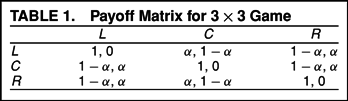
The payoff matrix for the game is given in Table 1, where A is the row player and D is the column player. The (unique) mixed equilibrium is solved in the standard way and yields the following pair of equilibrium strategies
To simplify notation, we denote the equilibrium (p*, q*), where p*=σCA and q*=σCD are the equilibrium probabilities that A and D locate in the center position, respectively. The probabilities of locating at L (or R) are therefore (1−p*)/2 and (1−q*)/2, respectively. Using this notation, the equilibrium is p*=(2−3α)/(2−α) and q*=α/(2−α).
This equilibrium solution has several interesting properties. First, note that since
, this implies that σLA≤σCA and σLD≥σCD. This implies the quality divergence hypothesis: The advantaged candidate is most likely to locate at the center, while the opposite is true for the disadvantaged candidate, who is more likely to locate on the extremes. This holds generally for all values of α.
Second, the comparative statics with respect to the uncertainty index, α, are very interesting and a bit surprising and counterintuitive. First, ∂p*/∂α<0, so that as uncertainty increases (or the electorate becomes more polarized) the advantaged candidate becomes more likely to adopt an extreme policy. Surprisingly, the opposite is true for the disadvantaged candidate. That is, ∂q*/∂α>0, implying that the disadvantaged candidate becomes more likely to adopt a centrist policy as uncertainty increases. In other words, as the polarization index increases, the advantaged candidate tends to move away from the center and the disadvantaged candidate moderates. This is {the polarization hypothesis}. In the extreme case, when
(i.e., the median is at one of the two extremes), both candidates mix uniformly over the three locations.
Finally, uncertainty benefits the weaker candidate. The equilibrium probability that D wins is given by:
The change in this equilibrium probability as α changes is found by computing the derivative of ΠD*(α), which is given by
The derivative is positive because
. Notice that if there is very little uncertainty (α close to 0), the disadvantaged candidate almost never wins. The probability D wins reaches its maximum value of
when
.
EXPERIMENTAL DESIGN AND PROCEDURES
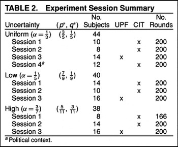
We conducted laboratory experiments using three values of α, corresponding to three levels of uncertainty. The three values were α=1/3 (uniform), α=1/5 (low uncertainty), and α=3/7 (high uncertainty). The experiments used students from the California Institute of Technology (CIT; Caltech) and Universitat Pompeu Fabra (UPF). Nine sessions were conducted, three for each value of α, of which two were carried out at CIT and one at UPF. Table 2 summarizes the information about each session. In addition, there was an additional Caltech uniform session run in a political context. The procedures are described in the next section.
Procedures
The experiments were conducted using software developed at the Hacker Social Science Experimental Laboratory at Caltech. The interface for the software presents each subject with a matrix of payoffs and keeps track of the history of previous game outcomes automatically for each subject. The matrix of payoffs was strategically equivalent to the three-location games, but constants were added to the payoffs to avoid zero outcomes and to approximately equalize the payoff magnitudes for A and D players.
Each session lasted 200 rounds, each round being one play of the game.16
The first High session was terminated after round 166 due to a computer crash.
Between eight and 16 subjects participated in each session. Total earnings were equal to the sum of all earnings over the 200 rounds. Average earnings were $20 and sessions lasted about 90 min.
17 For the experiments conducted at UPF, earnings averaged 13 Euros.
Each subject played both roles (A and D). At the beginning of the session, subjects were assigned to be either row or column players and instructions were read aloud. The game matrix was displayed in front of the room for everyone to see. It also appeared on their computer screen. In each round, row players clicked their mouse on a row to make a decision and column players clicked on a column to select their decision. After everyone had made a decision, the row/column outcome of their match was highlighted in the matrix on their screen. The screen also kept a display of the history of their play and the choices made by their past opponents. Several practice rounds were conducted in order to familiarize the subjects with the computer interface. During these practice rounds, the subjects were not allowed to make any choices on their own.
The subjects then played 100 rounds, being randomly rematched into pairs (one column player and one row player) after each round of play. After round 100, the payoff matrix was changed so that the row and column players' roles were reversed. That is, the column player's payoffs now corresponded to what a row player's payoffs had been in the first 100 rounds, and vice versa. This reversal was carefully explained to the subjects. They played 100 additional times with these reversed roles. This reversal allowed each row subject to have 100 rounds of experience as the A player and 100 rounds of experience as the D player, and the same for each column player. For all sessions except the political context session, the instructions were worded in neutral terms that would not be associated with personal political ideology. The three strategies were labeled A, B, and C. A sample copy of the instructions is given in the Appendix.
For the political context session, the subjects were told that they were adopting the role of political candidates, and they would be choosing policy platforms over a sequence of 200 elections. The number of votes they received in an election depended on their policy and the policy of the other candidate in the election. They were allowed to choose from a menu of three policies, generically called A, B, and C. The number of votes each candidate received as a function of pairs of policies (one for each candidate in the election) was determined in exactly the same way as the payoffs from the neutral uniform treatment. Subjects were paid a constant amount for each vote they received. As in the neutral context experiments, each subject played 100 times in the role of the A candidate and 100 times in the role of the D candidate. Therefore, this session was strategically identical to the other uniform treatments, the only difference being the political context.
Hypotheses
We have the following comparative static hypotheses that are derived from the theory. They are summarized below, denoting the empirical choice frequencies of center
and the treatments H, M, and L (for high, medium, and low uncertainty)
- .
- .
- for all uncertainty treatments.
This implies the following string of inequalities:
Summarizing, there are four primary hypotheses based on the Nash equilibrium model. The first hypothesis states that disadvantaged candidates will choose the center location less than one-third of the time, regardless of the level of uncertainty. The second hypothesis states that advantaged candidates will choose the center location more than one-third of the time, regardless of the level of uncertainty. Thus hypotheses 1 and 2 jointly imply the quality divergence hypothesis. The third hypothesis states that disadvantaged candidates will choose the center location more often as the level of uncertainty increases. The fourth hypothesis states that advantaged candidates will choose the center location less often as the level of uncertainty increases. Thus hypotheses 3 and 4 jointly imply the polarization hypothesis.
RESULTS
The main results of the paper have to do with the effect of the primary treatment variable (level of uncertainty) on the location decisions of the subject candidates. The key observation from the experimental results is that all four of the main hypotheses of the theory are strongly supported by the aggregate data from this experiment. The Nash equilibrium order of center choice relative frequencies,
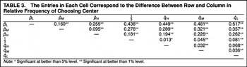
, is exactly what is found in the data. Table 3 clearly shows the support for all of these theoretical hypotheses. That table displays the differences between pairs of aggregate choice frequencies.18
For comparability reasons, the results presented include only data from the neutral context sessions. The findings from the political context session are discussed separately. However, it is important to note that none of the results change by pooling data from both contexts.
The cell entries in the table correspond to the difference in the relative frequency of center choices for two treatments (or one treatment compared with
. For example, the entry in the cell with row label
and column label
is
. Every single one of the 21 predicted differences has the correct sign, and all except one are statistically significant at better than the 1% level.
With the exception of the bimodal treatment, the aggregate fit for the A players to the quantitative prediction of Nash equilibrium was nearly perfect. The quantitative fit for the D players is not nearly as good, and the error was in the direction of overplaying the center strategy in all cases.19
Another quantitative feature of the data is that subjects do not play L and R with equal frequency. There is a small (but statistically significant) difference between R frequencies and L frequencies, for both A and D players, with R played more frequently than L.
The
A players overplayed the center strategy in two of three treatments (the exception being the
L treatment, where the difference is very small.) In addition, the
D players do not respond very strongly to the treatment effects. That is, the differences between
in the different treatments was always less than predicted by the theory. Thus, while the qualitative features of the data are very supportive of the theory, the actual magnitudes of
in the various treatments deviate somewhat from the Nash equilibrium predictions in systematic ways.
To summarize, there are seven main features of the aggregate data.
- The quality divergence hypothesis is strongly supported by the data.
- The polarization hypothesis is strongly supported by the data.
- All of the signed comparative static predictions about p and q are strongly supported by the data.
- All of these comparative static differences are statistically significant.
- The A player fits the Nash predictions much better than the D player.
- Both players tend to overplay the center strategy, and this effect is strongest for the D players.
- The response of the D players to changes in the level of uncertainty is less than predicted.
QUANTAL RESPONSE EQUILIBRIUM ANALYSIS
The strategic structure of equilibrium suggests the following possible explanation. If D players begin with uninformative prior beliefs about the choices by A players, then locating in the center is their optimal choice. The same is true for the A players. This could produce a pattern in which both players initially overplay C, then gradually adapt in the direction of their equilibrium strategy. Since in this kind of process D starts out farther away from his equilibrium strategy than A, it is not surprising that A frequencies are closer to their equilibrium values than D frequencies. What is needed to capture this idea theoretically is a model that can predict one player to be farther from Nash equilibrium than the other player.
QRE is an equilibrium model of imperfect play. A quantal response function is simply a smoothed out single-valued best response function that is monotonically increasing in expected payoffs. The quantal response functions are continuous and “statistical” in the sense that all strategies are played with positive probability. Therefore, players do not always play best responses. However, the monotone property implies that they play better strategies more frequently than worse strategies. Formally, for each player, the quantal response function maps the vector of expected payoffs of feasible actions into mixed strategy, which satisfies monotonicity and continuity properties. A QRE is a fixed point of the following composed mapping. Let σ be some (mixed) strategy profile in the game. Given σ, one can compute, for each player i and for each of player i's possible actions j, the expected payoff from playing that action, given σ, denoted Uij. Given these vectors of expected payoffs, the quantal response functions of players then yield a new mixed strategy profile,
. A QRE is a fixed point of this mapping, that is, a mixed strategy profile, σ*, with the property that
. McKelvey and Palfrey (1995) establish a number of theoretical properties of QRE points, including existence and upper hemicontinuity and a connection between QRE and Bayesian equilibrium of games with payoff disturbances.
A particularly useful parametric form of QRE is the Logit equilibrium. The Logit equilibrium arises when all players' quantal response functions are Logit functions of the expected utilities that are implied by the mixed strategies.
20 Hence the Logit equilibrium is the game theoretic extension of the standard Logit model of discrete choice that is commonly employed in empirical estimation of individual choice models. See McFadden (1976) for a survey of the Logit and related models of quantal choice.
Formally, a Logit quantal response function is given by
where λ is a parameter measuring the responsiveness of i to payoff differences between strategies. A Logit equilibrium is therefore a mixed strategy profile σ* such that
When λ=0, behavior is completely random, and the unique Logit equilibrium has every player choosing actions according to a uniform distribution. When λ→∞, the Logit equilibria converge to Nash equilibria. The Logit equilibrium correspondence for a game is the set of all Logit equilibria for the game, for each nonnegative value of λ. Because of its simple functional form, Logit equilibria are relatively easy to compute numerically and, in some cases, analytically. Gambit software (1999) was used for the calculations and figures above.
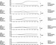
Figure 1 displays the graphs of the Logit equilibrium correspondences for each of the primary treatments. Logit equilibrium choice probabilities are on the vertical axis and λ is on the horizontal axis. Each graph has two curves, one for the probability of choosing center and a second that is the probability of choosing left (by symmetry equal to the probability of choosing right). From the graphs, one can see how the QRE captures the intuition that the A players converge more quickly to the Nash equilibrium, while the D players converge slowly. Neither converges monotonically. For intermediate values of λ, both players overplay C relative to Nash equilibrium.
The Logit equilibrium correspondence provides a structural model that permits us to fit the data to QRE using standard maximum likelihood techniques. Given a dataset consisting of n observations of A and D choices in the location game, one can construct the likelihood function as a function of the free parameter, λ, which is determined by the theoretical choice probabilities of the unique Logit equilibrium for that value of λ. The maximum likelihood estimate of λ is the value of λ at which that likelihood function is maximized. This parameter estimate in turn implies estimated equilibrium choice frequencies
using the formula above.
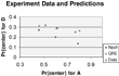
Figure 2 includes the fitted QRE-predicted choice probabilities of A and D, as well as the Nash predictions and the aggregate data. The QRE model clearly picks up the three anomalous features of the data: overplay of center by both players, the worse fit of D compared to A, and the weaker responsiveness by D to changes in uncertainty.
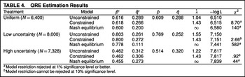
Table 4 presents the QRE estimates of the data broken down by treatment and model. Column 1 lists the three treatments, uniform, low, and high, and the number of observations of each treatment. We computed estimates for three models, which we call the unconstrained model, the constrained model, and the Nash model, respectively. The unconstrained estimates allow a separate estimate of λ for each treatment, while the constrained estimate forces
to be the same for all treatments. The Nash model computes the likelihood function using the Nash equilibrium choice probabilities, which correspond to the limit of the QRE choice probabilities when λ→∞.
Columns 3 and 4 give (
), the estimated choice probabilities under the various models. Columns 5 and 6 give (
), the empirical relative frequencies observed in the experiment.21
The data for QRE estimation include only observations from the neutral context treatment, in order to avoid confounding comparisons across the primary treatments (subject pool and distribution of voters). The estimates for those data are virtually the same as the estimates for the uniform treatment.
Column 7 gives the maximum likelihood estimate of λ, and column 8 gives minus the value of the log likelihood function for the model, evaluated at the maximum likelihood estimate of λ.
The constrained model is nested in the unconstrained model, so we use a likelihood ratio test to test for model rejection. The chi-square statistic (twice the log of the likelihood ratio) is given in the last column in Table 4. While the unconstrained model fits slightly better in all three cases, the improvement in fit is insignificant (at the 10% level) for two of the treatments (bimodal and unimodal). Only with the uniform treatment is it statistically significant (at the 1% level), but even for this case, the improvement in fit is of little real consequence, as the implied differences for choice probabilities between the two models are negligible.
The Nash equilibrium model is also (approximately) nested in the unconstrained model, so we can again use a likelihood ratio test to test for model rejection. The Nash model is easily rejected for all treatments, and the differences are statistically significant at any conventional level.
EXPERIENCE AND LEARNING
We investigate learning at a macro scale, simply asking whether aggregate behavior was different after subjects had a chance to observe the pattern of behavior of their opponents. Recall that our design used random matching, so that subjects were not trying to outguess an opponent based on observation of that opponent's play. Instead, the subjects were receiving information about he average play of the population over time. For this reason, this subsection focuses on changes in average play over the course of a session.
We divide the data into two data subsets; we call one experienced and the other inexperienced. Since subjects played 100 rounds in each candidate's role, we define inexperienced rounds to be the first 50 rounds a subject was in a particular round and define experienced rounds to be the remaining 50 rounds a subject was in that role.22
In the case of the experiment that crashed, we lost 34 rounds of experienced data.
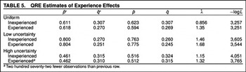
There were clear and significant trends in the data, with the experienced data being closer to Nash equilibrium and also fitting the QRE model better. Also, in all cases the estimate of
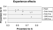
increases with experience, and the changes are significant at the 1% level or better. However, in most cases, the actual movement in the aggregate choice probabilities was not very large. Table 5 displays the estimates broken down separately by treatment and by experience level. Figure 3 compares the inexperienced and experienced data in a graph similar to Figure 2.
HETEROGENEITY, SUBJECT POOL EFFECTS, AND CONTEXT EFFECTS
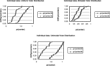
This section examines variation in choice behavior across subjects. We find evidence for heterogeneity. Even with the heterogeneity, all of the comparative statics results are still supported in the data. This is important to note because the statistical tests in the earlier section assume that all observations are independent, and therefore the significance levels are inflated. One way to adjust for this is to conduct similar tests with the individual-level data, comparing the population distribution of choice probabilities across samples, using nonparametric statistics. This is what we do here, with the pooled sample of individuals. Figure 4 shows the cumulative distributions of individual choice frequencies by treatment and by role. For example, in the uniform treatment, there were 32 subjects, so the graph shows 32 center choice frequencies for the individuals when they were A players and 32 choice frequencies for the same individuals when they were D players. Each point on the graph gives the relative frequency (of 100 moves) that a particular individual chose the center strategy in a particular rule. The points are ordered by relative frequency (not subject), so that the curves represent empirical cumulative distribution functions (CDFs) of individual choice frequencies. There is a clear ordering of these empirical CDFs as hypothesized. A second issue with heterogeneity arises because we used two separate subject pools.
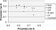
This feature of the design was implemented as a robustness check. The student populations (and culture) at UPF and CIT are different in many ways, but the theoretical model is intended to apply to both subject pools, so we do not predict a difference. Figure 5 displays the UPF and CIT data as well as the Nash predictions and the QRE estimates.
Indeed the behavior in the two subject pools is very similar, with some small quantitative differences. There is one reversal of the sign predictions, which occurs in the CIT data. That reversal is
, but the difference (−0.016) is not significant at the 5% level.
The uniform session conducted with a political context yielded results similar to those of the other uniform sessions. The relative frequencies for A and D locating in the center position were 0.652 and 0.278, respectively. This datapoint is displayed as a shaded triangle in Figure 5. To test for significant differences between this and the neutral uniform sessions, we used the Logit equilibrium as the structural model and conducted a likelihood ratio test between the constrained and the unconstrained estimates. The chi-square statistic is .88 with one degree of freedom, which is insignificant at all conventional significance levels (p≈.5).
CONCLUSIONS
The results of this laboratory experiment provide strong support for the theoretical equilibrium effects of candidate quality on policy location. The central predictions of the theory are the quality divergence hypothesis and the polarization hypothesis. That is, (1) both candidates diverge from the center, with the weaker candidate diverging more than the stronger candidate; and (2) as the distribution of voters becomes more spread out, both candidates moderate their positions. The design allowed us to test these key predictions about how endogenous variables (candidate locations) covary with candidate quality and with the distribution of voters. All of these predictions were supported by the data. Altogether, the design and the model offer 21 predicted sign differences in the observable choice frequencies by the candidates, across the three treatments. Every single one of these 21 predicted sign differences was the correct sign according to the theory, and all of these differences were statistically significant.
The quantitative predictions of the theory were also the right order of magnitude, but there were two interesting biases that were observed. First, we found that when subjects were in the role of the advantaged candidate they were more responsive to the changes in the distribution of voters than when they were in the role of the disadvantaged candidate. As a result the Nash equilibrium predictions fit the data for advantaged candidates better than the data for the disadvantaged candidates. Second, on average, subjects in both roles adopt more moderate positions than predicted by the model. We show that both of these observations can be accounted for very well by a bounded rationality version of Nash equilibrium, called quantal response equilibrium.
The experiment not only shows robustness of the model with respect to bounded rationality, but also demonstrates robustness of behavior across subject pools and with respect to experimental context. The latter is important for considerations of external validity of the results. Neither of the two secondary treatments (subject pool and context) had any effect on the qualitative conclusions of the experiment. The behavior in the two subject pools (from two different countries) was qualitatively identical and quantitatively very similar. Behavior in the political context treatment was not significantly different from behavior in the neutral context sessions. This suggests robustness of the basic game theoretic predictions of the model, at least with respect to these sorts of considerations, and this robustness leads us to be optimistic about its relevance to electoral politics.
APPENDIX: SAMPLE INSTRUCTIONS
Welcome to the SSEL Lab. Please do not do anything with the computer equipment until you are instructed to. Please put all of your personal belongings away, so we can have your complete attention. Raise your hand if you need a pencil. Feel free to adjust your chairs so they are comfortable for you.
This is an experiment in decision making, and you will be paid for your participation in cash, at the end of the experiment. Different subjects may earn different amounts. What you earn depends partly on your decisions and partly on the decisions of others.
The entire experiment will take place through computer terminals, and all interaction between you will take place through the computers. It is important that you not talk or in any way try to communicate with other subjects during the experiment.
We will start with a brief instruction period. During this instruction period, you will be given a complete description of the experiment and will be shown how to use the computers. If you have any questions during the instruction period, raise your hand and your question will be answered so everyone can hear.
During the computer instruction session, we will teach you how to use the computer by going through a practice session. We will go through this practice session very slowly and it is important that you follow instructions exactly. Do not hit any keys until you are told to do so, and when you are told to enter information, type exactly what you are told to type. You are not paid for the practice session.
We will first pass out the practice experiment record sheet, on which you will record all of the results from this experiment. Please record your name, the date, and your Social Security number on the bottom of the sheet. Note that you have been assigned a color, either Red or Blue. The color is written on top of the record sheet.
[PASS OUT RECORD SHEETS]
[WAIT FOR SUBJECTS TO RECORD INFORMATION]
[START PLDK SERVER PROGRAM ON SERVER, IF NOT DONE ALREADY]
Please click on the ICON that says “PLDK client.” When the computer prompts you for your name, type your full name, your Social Security number, and click on your color. Then click OK to confirm. If you have any questions about how to do this, please raise your hand.
[WAIT FOR SUBJECTS TO LOG ON]
You now see the experiment screen. You have each been assigned to be either a RED subject or a BLUE subject in this experiment. Your color as well as your subject ID number is shown in the banner at the top of the screen. Please record your subject ID number on your record sheet.
[WAIT FOR SUBJECTS TO RECORD INFORMATION]
Each of you has been matched by the computer with a subject of the opposite color. If you are a BLUE subject, you are matched with one of the other RED subjects. If you are a RED subject, you are matched with one of the BLUE subjects.
In the upper left part of the screen, you see a table.
[SHOW TABLE ON OVERHEAD PROJECTOR]
Will all subjects now move the mouse into the table and click it. If you are a RED subject, one of the rows will be highlighted. If you are a BLUE subject, one of the columns will be highlighted.
Each of you is asked to make a choice, but please do not do so at this time. If you are a RED subject, on the left of the screen you are asked to please choose a row. If you are a BLUE subject, you are asked to please choose a column. The outcome, and your payoff, is determined by the cell in the table that is chosen. In each cell of the table, the first number is the payoff for the RED subject, and the second number is the payoff to the BLUE subject.
[GO THROUGH A COUPLE CELLS IN OVERHEAD TABLE TO EXPLAIN]
[WAIT FOR SUBJECTS TO HIGHLIGHT ROW OR COLUMN]
Will all RED subjects now please choose “B” and all BLUE subjects please choose “A” by clicking the mouse button now while the arrow is pointing to the appropriate row or column. After you have made your choice, you are given a chance to confirm your decision. If it is not correct, please change it. When it is correct, please confirm by clicking on “confirm” now.
[WAIT FOR SUBJECTS TO CHOOSE AND CONFIRM CHOICE]
[WALK AROUND ROOM TO CHECK]
After all subjects have confirmed their choices, the match is over and you are shown the choice of the blue subject you were matched with. The outcome of the round, BA, is now highlighted in purple on everybody's screen. Your earnings are determined by the entries in the highlighted cell of the table that was selected. So the payoff to a RED subject for the first match is 6 points and the payoff to a BLUE subject is 14 points. You are not being paid for the practice session, but if this were the real experiment, then the payoff you have recorded would be money you have earned from the first match, in points.
We will now proceed to the second practice match. Each match is the same except you are matched with a new subject of the opposite color. Note that the decisions and payoffs of the first match are recorded in the experiment history at the right side of the screen. The outcomes of all of the previous matches will be recorded at the right side of the screen throughout the experiment so that you can refer back to previous rounds whenever you like.
[HIT KEY TO START SECOND ROUND]
For the second match, each of you have now been rematched with a new subject of the opposite color. All RED subjects again choose “B” and confirm. All BLUE subjects choose “C” by clicking on the right column.
[WAIT FOR SUBJECTS TO CHOOSE AND CONFIRM CHOICE]
The payoff to a RED subject for this practice round is 8 points and the payoff to a BLUE subject is 12 points. This concludes the second round. Notice that the results are again recorded in the history screen. Note also that the history screen keeps track of the number of times you have chosen each row or column, and of the average payoff you received from each row or column. For example, the red subject has chosen “A” twice. The first time she received 6, and the second time 8 points. So the average is 7.
[DO FOUR MORE ROUNDS, CHOOSING (BA), (CC), (BB), (CA)]
[HIT KEY TO END PRACTICE SESSION]
This concludes the practice session. The computer screen now indicates your total points that you earned in the practice session. This is multiplied by the exchange rate to get your money Payoff. Since this is a practice session, the exchange rate is zero. In the actual experiment, the exchange rate is 0.01, so that each point is worth one cent.
[WAIT FOR SUBJECTS TO RECORD OUTCOME AND CLICK “OK”]
Part 1
The actual experiment consists of two parts. Each part will last for 100 matches. When the first part is over, we will give you some additional instructions before the second part begins. Each match will proceed as in the first practice match, except you will be paid one cent for each point. The table will have three rows and three columns, the row and column labels will be the same as the practice, and the payoffs in the table will be the same as in the practice. Also, just like in the practice round, you will be randomly rematched with a new subject of the opposite color after each match.
The total amount you earn in this first part of the experiment is equal to the sum of your earnings in all 100 matches. You will be paid in cash at the end of the experiment. No other participant will be told how much money you earned in the experiment. You need not tell any other participants how much you earned. Are there any questions before we begin the experiment?
O.K., then we will now begin with the actual experiment.
Please lower your chairs to the lowest position, and pull out the dividers as far as they will go. This ensures your privacy and the privacy of the others in the experiment. We will now begin match number 1.
[START EXPERIMENT]
[AFTER FIRST MATCH ANNOUNCE:]
The first real match of the experiment is over. There will be 99 more matches in Part 1. Remember that you are randomly rematched with a new subject after every single match. After match 100 has finished, please record your total payoffs on your record sheet and then wait for the instructions for the second part of the experiment.
Part 2
This is the second and final part of the experiment. The amount of money you earn in this part will be added to the amount you earned in Part 1 to determine your total money earnings for the whole experiment. Just as in Part 1, each point is worth one cent. This part of the experiment is similar to the first part, except the payoff table has been changed in a very specific way.
[SHOW NEW TABLE ON OVERHEAD PROJECTOR NEXT TO OLD TABLE]
This is a payoff table that reverses the roles of Blue and Red. That is, Blue's payoffs are the same as Reds payoffs were in Part 1, and Red's payoffs are the same as Blue's payoffs were in Part 1. For example, suppose that Blue chooses A and Red chooses B. Then Blue gets 6 and Red gets 14. Now compare this to the payoffs in the first table, when Red chose A and Blue chose B.
[PUT UP COMBINED SLIDE WITH BOTH PAYOFFS]
Then Red got 6 and Blue got 14. If you look carefully at the new table, you will notice that it is derived from the old one by transposing it (that is, flipping it around the diagonal) and reversing the Red and Blue payoffs.
[ILLUSTRATE HOW THIS TRANSPOSITION WORKS USING OVERHEADS]
Are there any questions before we begin?
O.K., then we will now begin the second part. The second part will also have 100 matches. Remember that you are randomly rematched with a new subject after every single match. After match 100 has finished, please record your Part 2 total payoffs on your record sheet and then wait for instructions for how to be paid. We ask you to refrain from talking with each other, not only during the matches, but also while you are waiting to be paid. Thank you in advance for your cooperation.
[BEGIN SECOND PART]
[END AFTER MATCH 100]
The experiment is now over. Please record your Part 2 money earnings and add them to your Part 1 money earnings. Enter this sum in the row labeled Total Earnings. You will be paid this amount of money in the next room. We will pay you one at a time, beginning with subject number 1. We ask you not to talk with each other or use the computer equipment while you are waiting to be paid. Subject number 1, will you please come with us to the next room. Please collect your belongings and bring them and your record sheet with you. You will be leaving from the outside door in the next room.
Aragones acknowledges financial support from the Spanish Ministry of Science and Technology, Grant SEC2000-1186 and CREA. Palfrey acknowledges financial support from the National Science Foundation, Grants SES-0079301 and SES-0094800, and from the Hacker Social Science Experimental Laboratory at Caltech. The paper has also benefited from suggestions by three anonymous referees, the editor, and seminar audiences at Caltech, Columbia University, New York University, Princeton University, ITAM, GREQAM, the 2001 meeting of the American Political Science Association, the University of Malaga, and Universitat Pompeu Fabra.






Comments
No Comments have been published for this article.