


1. Introduction
Recent evidence suggests that the dynamics of Greenland glaciers are highly sensitive to external forcing. In response to the loss of its floating ice tongue, Greenland’s largest outlet glacier, Jakobshavn Isbræ, doubled in speed while retreating, thinning and increasing its calving rate (Reference JoughinJoughin and others, 2008). Helheim Glacier also experienced similar dynamic thinning and increases in speed along its main trunk, in response to retreat of the ice front (Reference Howat, Joughin, Tulaczyk and GogineniHowat and others, 2005). During the acceleration, the annual mass loss nearly doubled in 2004, but within a 2 year period (2006) decreased to near-previous rates, likely due to stabilization of flow near the terminus (Reference Howat, Joughin and ScambosHowat and others, 2007). The results suggest that ice dynamics, manifested in flow speed, glacier thickness adjustments and calving, are closely linked, with the ability to vary rapidly. Furthermore, grounded ice is likely sensitive to changes occurring at the terminus.
If ice dynamics can change rapidly in response to a warming climate, such changes may be directly related to ice/ocean interactions. Some of these changes may be driven by long-term oceanic warming present in the waters surrounding Greenland; one notable observation indicates an incursion of warm water around 1997 offshore of Jakobshavn Isbræ, which may have contributed to calving of its floating ice tongue and doubling in speed (Reference Holland, Thomas, de Young, Ribergaard and LyberthHolland and others, 2008). Further evidence from within fjords in southeast Greenland suggests that wind-driven exchange at the continental shelf drives subtropical waters into fjords, creating a circulation which brings warmer waters into fjords and increases melting at the terminus (Reference StraneoStraneo and others, 2010). Local fjord-scale tidal pumping can be another important heat delivery mechanism to consider (Reference Mortensen, Lennert, Bendtsen and RysgaardMortensen and others, 2011). A pervasive presence of warmer waters near the Greenland coast and throughout the Arctic may drive the observed reduction of sea-ice extent in the Arctic in the last decade (Reference Serreze, Holland and StroeveSerreze and others, 2007).
The decreasing summer extent of sea ice on the Greenland margin also suggests decreased sea-ice strength within fjords. At glaciated margins, landfast sea ice traps calved icebergs near the fronts of the glaciers, creating a compacted mixture of sea and calf ice. The term ice melange has been used to describe related ice conditions in various oceanographic settings (Reference Rignot and MacAyealRignot and MacAyeal, 1998; Reference Amundson, Fahnestock, Truffer, Brown, Lüthi and MotykaAmundson and others, 2010). This study focuses on a major outlet glacier in west-central Greenland, Store Gletscher, where the melange thickness may vary by hundreds of meters, depending on iceberg concentration. The melange is further strengthened in the winter by freezing and formation of sea ice in interstitial gaps between icebergs, before eventual break-up in spring. In this area, the ice melange reaches its peak extent in late April and disappears rapidly in May (Reference Howat, Box, Ahn, Herrington and McFaddenHowat and others, 2010). Plausibly, the ice melange strengthens seasonally, as sea ice grows, and bonds ice fragments with sea ice in the fjord, complicating attempts to generalize its rheology.
In fjords, the presence of an ice melange has oceanographic implications, such as preventing atmosphere–ocean heat and momentum exchange, which influences wind-driven mixing. Thus ice melange may provide a significant mechanical link between ocean conditions and glacier dynamics. Plausibly, the ice melange exerts some back-stress upon the glacier. Reference Amundson, Fahnestock, Truffer, Brown, Lüthi and MotykaAmundson and others (2010) infer that the ice melange is responsible for the seasonal cessation of calving at Jakobshavn Isbræ. Other observations suggest that the disappearance of multi-year landfast sea ice can lead to rapid calving at Greenland glaciers (Reference Reeh, Thomsen, Higgins and WeidickReeh and others, 2001). If climatic trends continue towards decreasing sea-ice concentrations and earlier break-up of sea ice at the Greenland margin, longer and less-obstructed calving seasons may persist and drive accelerated glacier flow and retreat.
To identify rapid changes in glacier behavior, we monitor changes in glacier flow speed using GPS and photogrammetry. The increasing use of high-rate, precise positioning has allowed the identification of tidal variations in velocity at ice streams (Reference Anandakrishnan, Voigt, Alley and KingAnandakrishnan and others, 2003; Reference Bindschadler, King, Alley, Anandakrishnan and PadmanBindschadler and others, 2003; Reference GudmundssonGudmundsson, 2007) and Greenland outlet glaciers (de Juan and others, 2010). Typically, ocean tides impart relatively small stresses on the order of tens of kPa. Therefore, the sensitivity of glaciers to small stress fluctuations may provide unique insight into flow characteristics, such as boundary conditions at the base.
These rapid changes in ice flow dynamics at the terminus are closely related to calving dynamics, so this study also includes observations of the relationship between loss of grounded ice to calving and the transient speed. The ever-changing terminus position is the balance between ice speed and calving rate (Reference Meier and PostMeier and Post, 1987). The key difficulty in understanding calving requires coupling physical mechanisms operating at different timescales; ice near the terminus cracks and cleaves away from termini in abrupt instants, while the glacier may change thickness or velocity, changing its terminus position on sub-daily to decadal timescales (e.g. Reference Howat, Box, Ahn, Herrington and McFaddenHowat and others, 2010), sometimes synchronous with changes in calving. A better understanding of calving dynamics would allow its parameterization in ice-sheet models and improve our understanding of future responses of marine ice sheets and glaciers to climate forcing.
In this study, we examine the influence of three glacier terminus processes on the sub-daily variations in the dynamics of Store Gletscher: (1) the break-up of the ice melange; (2) fluctuating oceanic tides; and (3) calving. We observe ice flow speeds near the terminus and 16km up-glacier and compare the sub-daily oscillations with tidal stage and the presence/absence of the ice melange. We develop a method of quantifying calving activity and compare it to the ice flow speed observations. The observations indicate that forcing at the terminus from these factors influences ice flow speeds further up-glacier, though quantifying the direct influence of any single mechanism in isolation proves limited.
2. Experiment Description and Measurement Techniques
A spring/summer 2008 field campaign was carried out at Store Gletscher, an outlet glacier that terminates in a ~70 km long fjord within the Uummannaq District on the central coast of West Greenland (Fig. 1). Store Gletscher has displayed no multi-year change in front position exceeding ~1.5 km in at least 40 years (Reference Weidick, Williams and FerrignoWeidick, 1995, p. C41). It does display a relatively small ±200mseasonal oscillation in front position (Reference Howat, Box, Ahn, Herrington and McFaddenHowat and others, 2010), likely due to growth and decay of a ~200m section of floating tongue. The advance typically occurs rapidly in April and May, reversing to a similarly brief period of rapid retreat once the melange clears. Average melt-season speeds remained stable between 2000 and 2009, with typically small (<10%) variation during the melt season, except for 2002 and 2005 when speed decreased 20–40% in midsummer. The glacier terminus widens toward the front to 5.2 km and flows 11–15md–1 at the front (Reference Ahn and BoxAhn and Box, 2010). A dual-frequency GPS receiver recording at 1 Hz was located on the ice ~16 km upstream of the terminus. An automatic weather station (AWS) was situated beside the on-ice GPS station. Air temperatures were recorded at heights of 1.5–2.0m using a fine-wire thermocouple sensor that is insensitive to solar heating. On-ice wind-speed measurements were made with an ultrasonic anemometer situated 0.5 m above the temperature sensor. Four medium-period (response is linear with ground velocity for periods from ~0.03 to 30 s) seismometers were located near the terminus on bedrock. A tide gauge was installed beside an island 9 km southwest of the terminus. Air temperatures presented in this paper were collected from the on-ice station. Time-lapse cameras, capturing images at 15 min intervals, were positioned on the north (one camera) and south side (two cameras) of the fjord, though only data from one of the south time-lapse cameras are utilized quantitatively in this study (Fig. 1). The other cameras provided the timing of changes in sea-ice state. In order to obtain near-terminus speed estimates from the repeat photos, we implemented the Multi-Image/Multi-Chip matching procedure (Reference Ahn and HowatAhn and Howat, 2011) applied to single-camera oblique photogrammetry of glaciers (Reference Ahn and BoxAhn and Box, 2010).
Location of the field site at Store Gletscher, with symbols denoting seismometers (red triangle), on-ice GPS station and co-located AWS (green inverted triangle, blue circle), time-lapse camera (yellow cross) and a tide gauge (blue circle).

3. Observations
3.1. Ice melange break-up
The time-lapse photos indicate the glacier calving front stabilizing and the glacier growing in length throughout the winter months and into spring. This seasonal ice melange rapidly disintegrates and clears within a few days in late May or early June in this region. Wind gusts above 25ms–1 observed on day 149 (28 May) contributed to the Store Gletscher ice melange break-up. The time-lapse photos indicate large bonded icebergs remobilizing and floating away from the terminus.
After the melange mobilizes, the fjord remains blanketed with an unbonded mixture of smaller bergs and brash ice (Fig. 2a). A small area of open water adjacent to the glacier front appears and persists at the southern terminus beginning on day 160 (8 June). This polynya has been observed in past years (Reference Weidick, Williams and FerrignoWeidick, 1995), and is a result of seasonal melt. The ice-front polynya continues to grow until around day 169 (17 June) when nearly the entire front of the terminus is clear of ice, with plumes of brown, sediment-rich water. While polynyas can also form at the front of Antarctic ice shelves due to cycling of warm oceanic waters beneath the shelf (Reference Mankoff, Jacobs, Tulaczyk and StammerjohnMankoff and others, 2012), the presence of brown, turbid water is indicative of meltwater plume originating at the glacier bed.
(a) A set of time-lapse images taken at ~7 day intervals showing the evolution of the terminus region. (b, c) The corresponding ice-speed records from (b) the on-ice GPS station, ~16km from the terminus, and (c) photogrammetry, near the terminus. The gray shaded region indicates break-up of the ice melange, as observed in the time-lapse images. (d, e) The period between days 145 and 160 is emphasized for (d) the on-ice GPS and (e) the near-terminus region.

3.2. Ice-Speed Observations
We use the oblique photogrammetric method (Reference Ahn and BoxAhn and Box, 2010) to estimate flow speeds near the terminus. Average errors are on the order of 0.5 md–1, evident as the amplitude of noise within the speed solutions. Speeds measured at the terminus are illustrated in Figure 2c and e. Figure 2c indicates that near-terminus speeds include peaks at semidiurnal and diurnal periods, though these solutions are noisy. In Figure 2d and e, we zoom in the period when the ice melange breaks up and the period immediately following it. Examination of both speed records indicates changes closely following the ice melange break-up around day 149 (28 May). After the break-up, the near-terminus ice undergoes an increase in speed of 14% (1.5md–1) over ~2 days (Fig. 2e).
The GPS data were post-processed in kinematic mode using the GAMIT/TRACK software package, to obtain differential positions relative to a bedrock station we deployed temporarily. In order to obtain reliable velocity estimates from the 1Hz position data, we smooth each position (Cartesian earth-centered, earth-fixed coordinates: x, y and z) using a 1 hour running mean and remove all points greater than 1σ from the running mean. Such a cut-off is necessary for high-sample rate data. The data are then down-sampled to 5 min medians, in order to increase computational efficiency, and a first-degree loess filter is applied with a 6 hour window. Figure 2b shows the along-flow horizontal speed.
The GPS record shows little variability until day 148 (27 May), with the exception of several, discrete speed-up events lasting several hours. A dense ice melange filled the fjord and air temperatures were below freezing for most of this period, and supraglacial meltwater accumulation was not visible on the ice surface. Between days 148 and 152 (27 and 31 May), the speed decreased ~15% as the melange cleared, exposing patches of open water. This clearing coincided with a sustained high-wind (30 min averages of 10ms–1 with 24ms–1 gusts observed at the on-ice AWS situated beside the GPS site) event lasting all of day 148 (27 May), when we observed large, tabular icebergs moving away from the front. During this period, speeds near the terminus increased ~1.5md–1, plausibly in response to loss of buttressing.
Following the ice melange break-up, the ice speed 16 km upstream from the terminus begins to undergo large diurnal and smaller semi-diurnal fluctuations. In order to evaluate the periodicity on the GPS record, we first perform a fast Fourier transform on the entire length of the flow speed record, which clearly identifies peaks at ~12 and ~24 hours (Fig. 3c). A spectrogram of the GPS flow-speed record highlights the timing of the presence of semi-diurnal and diurnal oscillations. A 6 day moving window evaluated at 1 hour increments produces the time series illustrated in Figure 3a. Warm colors (red) in Figure 3a indicate greater signal power at those periods. After the ice melange breaks up, dominant signals in the GPS data appear at both semidiurnal (~12 hour) and diurnal (~24 hour) periods. The semi-diurnal signal continues until day 156 (5 June), when it returns to background noise levels, then reappears on days 159–170 (7–18 June) through to the end of the record. The diurnal signal is strongest during days 150–159 (29 May to 7 June) and 164–170 (12–18 June). For the near-terminus estimate of speed, positive speed fluctuations occur at similar periods (Fig. 2b; 4 hour image pair data), though amplitudes of the speed increases in Figure 2e are artificial due to errors on the order of 0.5 md–1.
(a) Spectrogram of the ice speed observed at the GPS station, ~16km from the terminus. (b) The speed record for reference. After about day 150 (break-up of the melange), the ice speed is more strongly periodic about semi-diurnal (~12 hours) and diurnal (~24 hours) periods, which correspond to ocean tides. (c) The spectra of the entire speed record over the period of observation, exhibiting peaks at the same semi-diurnal (~12 hour) and diurnal (~24 hour) periods.

Large-amplitude ice-flow-speed fluctuations observed at the GPS station, during days 152–160 (31 May to 8 June), occur at low tides (Fig. 4a and b). However, the speed peaks also coincide with maximum daily air temperature (Fig. 4c). During this period, air temperatures over the ice were 0–5˚C during sunlit periods, with nights below freezing temperatures. Thus, meltwater production will have ceased each night, likely contributing to the strong diurnal periodicity of the speed increases. In a simple model of glacier response to climate, high air temperature enhances surface melting, increases meltwater that pressurizes the basal interface, and likely drives accelerated ice flow. In considering the effect of air temperature influencing ice dynamics, it should be noted that the air temperature likely increases toward sea level. Therefore, our on-ice measurement point may be considered a minimum air temperature, compared to those occurring down-glacier towards the terminus. While speed response to peak air temperatures or maximum solar insolation may lag air-temperature maxima by 7–8 hours (Reference Walters and DunlapWalters and Dunlap, 1987), we find nearly zero time lag for ice speed (Fig. 4). Such a small lag might be expected for temperature-driven speed increases because the GPS station is located immediately adjacent to a large supraglacial lake (the dark feature a few km northwest of the GPS station in Fig. 1). The air temperature exhibits diurnal peaks in its spectra, and not the semi-diurnal peaks observed in the GPS, time-lapse camera and tide-gauge data.
Measurements during days 140–170 of (a) ice flow speed, from the on-ice GPS stations ~16km from the terminus, (b) measured tide in the fjord and (c) air temperature measured at an AWS co-located with the GPS station.

The clear diurnal variation in speed and coherence with the air-temperature record suggests the development of a hydrologic connection between the surface and the bed. A diurnal oscillation of similar amplitude was also observed on Columbia Glacier, Alaska, USA (Reference Kamb, Engelhardt, Fahnestock, Humphrey, Meier and StoneKamb and others, 1994; Reference MeierMeier and others, 1994). This variation in motion, in-phase with air temperature, is consistent with observations of alpine glaciers, where a lag is attributed to thermal inertia of the surface and the time needed for water to flow from the source area to the glacier water table (Reference Mair, Nienow, Sharp, Wohlleben and WillisMair and others, 2002). During the period of strong diurnal periodicity (days 152–160 (31 May to 8 June)), no meltwater plume is visible at the ocean surface near the front, suggesting that drainage was relatively inefficient. The diurnal variation in meltwater penetration to the bed will then induce a cyclical perturbation to the basal water storage, causing sliding (Reference Kamb, Engelhardt, Fahnestock, Humphrey, Meier and StoneKamb and others, 1994). The peak daily amplitude in speed decreased after peaking on day 153 (1 June), disappearing after day 159 (7 June), despite the fact that air temperatures remained above freezing. This indicates a progressively decreasing influence of diurnal variations in surface meltwater input to the bed on local basal water pressure and sliding. This decrease could be due to increasing efficiency of the basal drainage system. Such a mechanism would result from the formation of a tunnelized drainage system, in which sliding becomes decoupled from basal water discharge (Reference RöthlisbergerRöthlisberger, 1972).
Due to the timing of our observations, it is impossible to explicitly isolate and identify periodic forcing contributors (low tide and high air temperature) that oscillate at nearly the same period and whose phase is nearly coherent. However, the presence of semi-diurnal periodicity in the speed record and not in the air-temperature data suggests that ocean tides influence the glacier flow dynamics. In addition to the periodic tidal and meltwater forcing of ice flow speed described above, in the following we consider the correlation between calving and flow-speed increases, by first developing a seismically determined time series for calving activity.
3.3. Seismic identification of calving
Various studies identify calving and glacier-related processes occurring across a broad spectrum of frequency. At Columbia Glacier, Reference O’Neel, Marshall, McNamara and PfefferO’Neel and others (2007) find peak iceberg calving energy, within 1–3 Hz, shifting to ~10 Hz after retreating into a deeper area (Reference Walter, O’Neel, McNamara, Pfeffer, Bassis and FrickerWalter and others, 2010). Seismicity observed for glaciers over a range of ice-thermal conditions (temperate, polar, etc.) may generate seismic radiation over a range of observable frequencies, including ~200 Hz (Reference Anandakrishnan and BentleyAnandakrishnan and Bentley, 1993), 6–35 Hz (Reference West, Larsen, Truffer, O’Neel and LeBlancWest and others, 2010) and 30–60 s (Reference Ekström, Nettles and AbersEkström and others, 2003; Reference Wiens, Anandakrishnan, Winberry and KingWiens and others, 2008; Reference Walter, Brodsky, Tulaczyk, Schwartz and PetterssonWalter and others, 2011). The large range of observations may be due to differences in equipment quality and distance from the source, though more likely due to the characterization of a variety of phenomena and, by extension, a variety of source mechanics. For example, Greenland glacial earthquakes have been described as occurring nearly synchronously with large calving events (Reference Tsai, Rice and FahnestockTsai and others, 2008), while similar events occur as basal sliding events on Whillans Ice Stream, West Antarctica (Reference Bindschadler, King, Alley, Anandakrishnan and PadmanBindschadler and others, 2003; Reference Wiens, Anandakrishnan, Winberry and KingWiens and others, 2008; Reference Walter, Brodsky, Tulaczyk, Schwartz and PetterssonWalter and others, 2011).
We develop a method of identifying bursts of calving activity within our seismic record, by first focusing on the nature of seismicity from a single calving event. The 15 min photos indicate a number of large, isolated calving events (e.g. Fig. 5a). Figure 5b illustrates the seismic record during the period spanning the two images for the east component of the southern seismic station, co-located with the camera. We compute the velocity spectra of two 100 s portions of the seismic record (Fig. 5c). The spectrum for the signal is generally fairly broadband, with a possible peak around ~1 Hz. Given the observation that the seismic signal is of significantly greater amplitude over a broad range of frequencies extending from ~0.3 Hz to the Nyquist frequency, we use the signal in this range to distinguish potential calving events. Computing the velocity spectra in 80 s windows with 50% overlap for all the stations in the network and stacking them produces the spectrogram in Figure 6a.
(a) Pair of time-lapse photos indicating a calving event occurring in the left third of the frame. (b) The east component seismic record from a station co-located with the time-lapse camera. We compute spectra for windows of 100 s during two periods, shown as signal and noise. (c) The spectra indicate increased energy above noise levels from ~0.3 Hz to the Nyquist frequency.

(a) Plot of the computed spectrogram for the stacked east components of the four stations within the network. Based on examination of the time-lapse photographs, calving events occur during vertical streaks of color above 5 Hz. To limit the amount of noise in a calving activity time series, we choose a frequency band between 7 and 20 Hz. We sum the energy within this band, take the logarithm and smooth the time series using a 1000-point window running average, in order to obtain the calving time series (b).

After identifying the largest calving events from the time-lapse photos, we find that the calving events occur synchronously with the concentrations of energy clearly visible as vertical bands in Figure 6a. The largest calving events in the time-lapse photos occur within one or two frames, constraining their duration to be 15–30 min. This is in contrast to the duration of calving activity in the seismic record, which can be on the order of hours. The difference in durations is possibly due to small fracture events (on the order of meters), which are recorded seismically but are not visible due to obstructions below the resolution of the camera. In order to avoid noise clearly visible in Figure 6a just below 5 Hz, we sum the cumulative energy within the 7–20 Hz band, take the logarithm, and smooth over a 1000-point running average (Fig. 6b). The peaks in the time series indicate discontinuous periods of intense calving activity.
The timing of the ice melange break-up is clearly visible near the beginning of the calving activity record (Fig. 7a) and abruptly ceases around day 150 (29 May), coinciding with the clearing of the ice melange. Especially around day 154 (2 June) and continuing through day 160 (8 June), some larger peaks in calving appear to be coherent with peaks in speed. With a moving 2 day sample interval, we find positive correlations during days 150–165 (29 May–13 June) (Fig. 7c) that indicate coherence between calving activity and ice-speed increases, which are more common after the ice melange break-up. Close examination of the calving record indicates that during days 154–156, near-terminus ice flow speeds lead calving activity by several hours. Due to the limited period of observations, we are hesitant to conclude causation, yet this timing suggests that speed increases near the terminus can cause calving. Such a hypothesis could be the subject of future study.
(a) The calving activity record from Figure 6b, which is the cumulative seismic energy of the east–west component in 7–20 Hz band for the four seismometers. For comparison, we also show (b) the GPS ice-speed record ~16km from the terminus. The gray shaded region indicates the ice melange break-up. Following a brief period of relative quiescence, peaks in the calving activity record and speed perturbations appear to be coherent during some days. We compute (c) a zero-lag correlation coefficient as a function of time, using a 2 day moving window. Positive correlations suggest periods when calving and speed perturbations are coherent.

4. Discussion
We have thus far presented evidence of external forcing of glacier dynamics by two oceanic mechanisms at the ice front, ocean tides and the absence/presence of the ice melange, and one internal glacial mechanism, calving. Meltwater production also likely perturbs ice flow speed, clearly manifested by strong diurnal speed increases following the ice melange break-up (Fig. 4).We reiterate that due to the nearly coherent phase of our observations, we cannot explicitly evaluate the contribution that each forcing makes to the flow speed. What follows are order-of-magnitude estimations of the expected flow speed increase in response to tides and the buttressing stress that restrains glacier flow when the melange is present. We observe semi-diurnal periodicity in the ice flow speed at the GPS station, which is indicative of tidal forcing. In Section 4.1 we use longitudinal coupling theory (Reference Echelmeyer and KambEchelmeyer and Kamb, 1986) to evaluate the expected amplitude of ice flow speed changes from a 2 m change in tide height. In Section 4.2, we quantify the ability of the ice melange to resist ice flow, by calculating the buttressing stress. This calculation relies upon the observation of a ‘ramped’ step-change in ice flow speed observed near the terminus, coincident with the removal of the ice melange. In Section 4.3, we give further context to the observational link between ice flow speed and calving.
4.1. Longitudinal coupling of ice flow by ocean tidal forcing
We begin our consideration of the oceanic mechanical perturbation of ice flow by predicting the glacier ice speed change in response to tides. A seminal paper by Reference Echelmeyer and KambEchelmeyer and Kamb (1986) introduced a rigorous analysis of longitudinal coupling of flow within a glacier. In addition to the typical force balance of a glacier, which can include the driving stress, lateral shear stress (wall stress) and basal shear stress terms, the longitudinal stress determines how the glacier responds to actions such as stretching. Reference WaltersWalters (1989) extended the longitudinal coupling theory to predict the flow response to a hydrostatic stress change due to tides at the terminus of Columbia Glacier. In the Appendix, we summarize some of the steps taken by Reference WaltersWalters (1989) to arrive at a solution for the flow speed increase from a tide change:

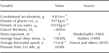
where u 1 is the perturbation velocity, p T is the pressure variation due to the 2 m tide level change (~20 kPa), η is the average effective viscosity, x is distance along-flow and L is the longitudinal coupling length-scale. For Eqn (1), we use the range of average effective viscosities from 0.5 to 2.0 bar a (1.58×10¹³ to 6.32×10¹³ Pa s), as found in Reference Echelmeyer and KambEchelmeyer and Kamb (1986). We determine the coupling length, L, via Eqn (A7). Other assumed values used for solving Eqn (1) are shown in Table 1 and the Appendix.
In addition to showing the predicted speed perturbations by tidal forcing in Figure 8, we also calculate the range in amplitudes of speed perturbations ~16 km up-glacier during the period 29 May–8 June (days 150–160). As illustrated in Figure 8, the predicted values for a 2 m tide lie within the range of observed speed perturbations for the m= 3 stress exponent. However, the maximum observed speed perturbations are nearly double the predicted speed perturbations from tidal forcing alone. Therefore, we hypothesize that the presence of meltwater also contributes significantly to the observed speed perturbations, especially during days 150– 160 (29 May–8 June). The amplitudes of the diurnal speed perturbations appear to decay during this period and later become less diurnally periodic, as the melt season continues. Coincidentally, the reduction in coherence between air temperature and diurnal speed perturbations (Fig. 4) coincides with the appearance of the polynya at the ice front on day 160 (8 June). Therefore, one plausible explanation is that when efficient drainage pathways develop, they lose their ability to pressurize the glacier bed.
Expected ice-speed perturbations, for a range of viscosities and stress exponents and their propagation along-flow, given a 2 m change in the tide at the terminus. The range in perturbation amplitudes for days 150–160 for the diurnal speed increases from on-ice GPS (Fig. 2d) is shown, and fits speed perturbation solutions for the stress exponent m =3.

Recent modeling results suggest that ice flow coupling can extend as much as 15–20km longitudinally inland from speed increases at the Greenland ice margin (Reference Price, Payne, Catania and NeumannPrice and others, 2008). We calculate coupling lengths, L, for various stress exponents and a range of potential effective viscosities of ice (Table 2). With a stress exponent of m= 3, we calculate a longitudinal coupling length, L, of 10–20km over the range of viscosities used (Table 2). This is a factor of 17–33 (L/H i) times the presumed thickness of the glacier near the terminus, H i (600 m). Reference Echelmeyer and KambEchelmeyer and Kamb (1986) suggest that glaciers in surge (e.g. the surging behavior exhibited at Variegated Glacier, Alaska) may reach values of L=H i ~12. Such a discrepancy may be reconciled by the fact that the Reference Echelmeyer and KambEchelmeyer and Kamb (1986) longitudinal coupling analysis does not account for basal sliding, which is plausibly a large component of the observed positive speed peaks.
Values computed for longitudinal coupling length, L, and velocity perturbation at the terminus, u 1(x 0), for a range of viscosities. The range of viscosities was chosen based on the original work (Reference Echelmeyer and KambEchelmeyer and Kamb, 1986; Fig. 3)

4.2. Ice melange buttressing stress from near-terminus ice flow speed increase
Here we use Eqn (1) to quantitatively estimate the strength of the ice melange. The melange strength likely continually evolves over winter and also may be dependent upon the amount of calved icebergs and their thicknesses within the fjord. However, the coincidence of the increase in speed observed at the front and clearing of the melange (Fig. 2), without substantial retreat of the ice front, suggests that melange directly resists ice flow.
Equation (1), at the limit of x = 0, reduces to an expression relating a velocity perturbation to a change in stress at the terminus front. If we rearrange this equation and assume that the pressure is derived from the presence/absence of the ice melange, we have

where the pressure due to the presence of the ice melange, p melange, is proportional to the velocity perturbation observed at the terminus, u 1(x 0), multiplied by the average effective viscosity, η, divided by the longitudinal coupling length, L. The along-flow length scale, L, is necessary because we are evaluating the longitudinal ice flow response to the removal of the ice melange buttressing effect at the terminus. The ice melange pressure, p melange, is conceptually equivalent to glacier buttressing or back-stress exerted by the melange. In evaluating the ice melange buttressing stress, we use the observed ~1.5md–1 increase in near-terminus ice speed as the value for u 1(x 0), as seen in Figure 2c (from photogrammetry dataset). We use the same range of effective viscosities as discussed in Section 4.1. With the stress exponent m= 3, we calculate buttressing stresses in the range 28–56 kPa. Thus, for a range of effective viscosities, we conclude that the winter sea-ice melange provides an effective back-stress, p melange, upon the glacier of ~30–60 kPa. The ice melange buttressing stress is not much larger than that induced by the range of tides observed at the terminus (20 kPa).
One way to quantify the relative significance of the melange buttressing stress is to compare the value to Store Gletscher’s driving stress. Driving stress is equal to ρgH i sin α, where α is the estimated surface slope and the other variables are the same as before. From the examination of satellite imagery, we estimate a change in slope of ~400m over ~10 km, or ~0.04. From these values, we calculate a driving stress of ~200 kPa. Our range of calculated melange buttressing stress (~30–60 kPa) is an order of magnitude less than the driving stress. The ice melange buttressing stress can be considered an additional seasonal resisting force and may be similar in magnitude to the basal drag resistance. These values for the seasonal buttressing back-stress are consistent with a few recent studies. First, when modeling the influence of the seasonal ice melange on calving, Reference Nick, Van der Veen, Vieli and BennNick and others (2010) used a value of 20 kPa for the back-stress imposed by the melange. Also, Reference Van der Veen, Plummer and StearnsVan der Veen and others (2011) directly applied a force-balance scheme to estimate a change of 150 kPa in back-stress, due to the loss of the floating ice tongue at Jakobshavn Isbræ from 1995 to 2005.
4.3. Calving and ice speed
The ice melange disintegration and associated calving are present in the record, starting on day 145 (24 May) and ceasing by day 150 (29 May). A short period of relative quiescence is observed until around day 154 (2 June) when calving continues periodically through the observation period. From day 154 to day 160 (2–8 June), peaks in calving are better correlated with peaks in flow speed (Fig. 7c). Near-terminus ice-flow-speed increases appear to lead calving activity by several hours during days 154–156, though accurately identifying timing is significantly hindered by smoothing of the calving activity time series and a noisy photogrammetry dataset. We merely point out that the calving and ice-speed increases are clustered in time, an observation made at other Greenland outlet glaciers (Reference NettlesNettles and others, 2008).
A correlation between calving and ice flow speed may be expected, as glacier velocity probably has important controls on calving. For ice shelves, Reference AlleyAlley and others (2008) show calving rate linearly correlates with a normalized stretching rate. Another model for calving productivity involves crevasse-depth criteria (Reference Benn, Warren and MottramBenn and others, 2007), where the calving margin is defined as the point where the crevasse depth equals the glacier freeboard. Therefore, if longitudinal stretching occurs under positive speed increases, then crevasse depth increases, promoting calving. Though a feedback between the two is expected, the identification of a causal link between calving and ice flow speed requires denser along-flow speed observations and a calving activity time series whose amplitude correlates with calved ice volume.
5. Summary and Conclusions
We have examined a number of short-term (sub-daily) variations in the flow dynamics of a major West Greenland ice-sheet tidewater outlet glacier. We obtained data from seismometers, GPS, time-lapse cameras and an on-ice automatic meteorological station. We observe two modes of oceanic forcing upon the glacier horizontal speed, the presence/absence of ice melange and ocean tides. Acceleration near the terminus of ~1.5md–1 (14%) over a 2 day period occurs after the winter sea-ice melange disintegrates and drifts away. Based on this ‘ramped’ step-change in speed, we determine that when the melange is present, it provides a ~30–60 kPa back-stress upon the glacier terminus, in the direction opposite ice flow. After the melange breaks up, we observe a synchronicity between flow speed, minimum ocean tidal range, and surface air temperature.
We find that the GPS ice-flow-speed time series includes both semi-diurnal and diurnal peaks; semi-diurnal peaks can only be caused by tides and are evidence that tides can influence flow at least ~16 km from the terminus. Further, we find that predicted speed increases match our observations of speed increases during this period, though only near the minimum range of GPS fluctuations. The discrepancy between observed and predicted speed perturbations, via the tidal range input to the longitudinal stress balance, suggests that melting likely contributes to the observed accelerated flow. The glacier likely undergoes a rapid flow response to melt lubrication via basal pressurization that exists for ~10 days. The drainage efficiency seems to increase to the point that basal pressurization is abruptly lost, followed by no correlation between horizontal speed and surface melting. The flow regime instead becomes characterized by a sustained correlation with semi-diurnal forcing from the tidal stage. Thus, we find evidence of an evolution in the relative importance of melt and tidal forcing, with further investigations planned for future field seasons.
Lastly, we show that calving and ice flow speed observed ~16 km upstream from the terminus appear to be manifested in nearly synchronous perturbations after the melange has been removed. The buttressing effect of the melange plausibly reduces longitudinal stretching, and its removal signals a period of increased susceptibility to calving.
Acknowledgements
We thank Jason Amundson and an anonymous reviewer for thorough and insightful reviews, which greatly improved the manuscript. Francis Nimmo and Eric Rignot are also thanked for enlightening discussions regarding the strength of ice melange. J.I.W. is funded by a NASA Graduate Earth and Space Science Fellowship. A University of California Institute of Geophysics and Planetary Geophysics Mini-Grant to J.I.W., a Special Research Grant from the UCSC Committee on Research to S.T., and a supplement to NASA grant NNX08AD31G-05 to S.T. provided partial support for field logistics. Funding for the GPS, time-lapse camera equipment and partial field logistics was made possible by an OSU Climate Water Carbon Initiative grant managed by Doug Alsdorf. Field logistics were also partially supported by NASA and the US National Science Foundation. We thank Dan Sampson for technical assistance prior to fieldwork, and Tristan Rhodes for assisting in preparing equipment. Uummannaq Polar Institute, managed by Ole Jorgen Hammeken and Ann Andreassen, assisted the field team.
Appendix: Longitudinal Coupling of Ice Flow Modulated by Tidal Stresses
In order to better understand external forcing at the terminus and its effect upon the glacier, we must first sum all the relevant stresses contributing to glacier flow. We follow the convention common in glaciology where stresses are geometrically corrected so that they are contact-area normalized. We assume that the sum of the driving stress, τ d, minus the longitudinal stress, τ L, and basal shear stress (basal drag), τ b, balances. Thus,

In order to evaluate the ice-flow-speed response to tides and compare with our observations of semi-diurnal and diurnal speed oscillations, we choose a relationship of velocity to basal shear stress and effective pressure. We employ a commonly used power-law sliding relation after Reference BindschadlerBindschadler (1983),

where u is horizontal velocity, k is an empirical constant and m is a locally determined exponent, either 1 or 3, best-fit with a value of 3 for most glaciers (Reference BindschadlerBindschadler, 1983). Effective pressure, p e, in Eqn (A2) is the ice overburden minus water pressure at the terminus and is positive for grounded ice. We assume, informed by the camera observations, that the glacier is grounded at the bed once the winter break-up has occurred. In this case, the effective pressure is thus always greater than zero, and is given by

where h w is the depth of the fjord at the terminus.
At this point, we follow the derivation of Reference WaltersWalters (1989), which is an application and extension of the derivation for longitudinal coupling by Reference Echelmeyer and KambEchelmeyer and Kamb (1986). For brevity, we do not repeat all the steps involved in this derivation. In introducing the derivation, we define our reference frame, where ice flows in the x direction. The force balance from Eqn (A1) becomes

The first term on the left-hand side (LHS) is the gravitational driving stress of the glacier. The second term on the LHS describes the longitudinal stress component of the force-balance equation. As most of the motion is dominated by sliding, ice rheology is further simplified, by assuming that a depth-averaged viscosity or effective viscosity, η, is sufficient. In addition, our assumption averages over along-flow length scales, and the average viscosity term is valid assuming du/dx does not significantly change along-flow, such as if there were no large variations in slope or thickness. Satellite imagery does indicate an undulating topographic variation in slope, likely also manifested as undulations in the basal topography. Significant variations of basal topography pose several complications in applying the assumptions for Eqn (A4) (Reference Echelmeyer and KambEchelmeyer and Kamb, 1986) and, as a result, our later predictions may be poor.
In order to further simplify Eqn (A4), Reference WaltersWalters (1989) uses perturbation analysis, where velocity, u, and effective pressure, p e, are expanded in terms of a mean plus a small perturbation. Expanding Eqn (A4) and collecting terms on the order of only the small perturbations results in

where x is distance along-flow, u
1 is the perturbation velocity, u is the average flow speed, η is the average effective viscosity, p
1 is the perturbation effective pressure, p
0 is the average effective pressure and τ
0 is the average basal shear stress. If we assume that H
i and η are relatively constant along-flow and  then Eqn (A5) reduces to

The longitudinal coupling length, L, is derived by Reference Echelmeyer and KambEchelmeyer and Kamb (1986) and is shown below, where m is the stress exponent, H i is the thickness of ~600 m, τ 0 is the average basal shear stress (150 kPa from Reference WaltersWalters, 1989) and u is the average flow speed near the terminus, or 11md–1 (Howat and others, 2010):

If basal water-pressure fluctuations are neglected (p 1 = 0), a solution to Eqn (A6) can be found that is an exponential function, which predicts the decay of near-terminus velocity perturbations as they propagate up-glacier.

Equation (A8) predicts horizontal speed perturbations as a function of distance from the terminus, where u 1 is the perturbation velocity and p T is the pressure variation due to the 2 m tide level change (~20 kPa).



