





Highlights
What is already known?
Previously described models have enabled the inclusion of both individual participant data (IPD) and aggregate data simultaneously in a network meta-analysis (NMA).
What is new?
We describe extensions to IPD and aggregate data NMA models that enable the estimation of component effects within the interventions. In addition, we further extend the models to adjust for covariates at the study-level and individual-level.
Potential impact for RSM readers
The proposed models could benefit those conducting evidence syntheses to inform economic decision models and future trial design. By incorporating more of the available evidence, they have the potential to enhance the evaluation of complex health interventions and support personalised, evidence-based recommendations for healthcare decision-making.
1. Background
Network meta-analysis (NMA) is a powerful tool in evidence-based research, allowing the comparison of multiple interventions by combining direct head-to-head evidence with indirect evidence.Reference Higgins and Green 1 However, in recent years, component NMA (CNMA) has emerged as an extension to NMA that can estimate the effects of individual components and their combinations within complex interventions. CNMA was originally developed in a Bayesian settingReference Welton, Caldwell, Adamopoulos and Vedhara 2 and later in a frequentist setting.Reference Rücker, Petropoulou and Schwarzer 3 There are several benefits of CNMA that make it desirable to researchers and decision makers, which have resulted in its increased application in recent years.Reference Pompoli, Furukawa, Efthimiou, Imai, Tajika and Salanti 4 – Reference Hartmann-Boyce, Ordóñez-Mena and Livingstone-Banks 13 Often, within an evidence synthesis, the included studies have not directly compared every combination of components as there are too many component combination options. CNMA overcomes the need to obtain direct study evidence for every component and possible component combination. The results provide useful evidence-based predictions for intervention effectiveness which can inform future research targeting the most cost-effective multicomponent interventions. CNMA can also provide more precise intervention effect estimates than NMA because the models use evidence of components across study arms, which is especially useful for sparse networks of evidence.Reference Thorlund and Mills 14 Additionally, CNMA can connect disconnected networks when there are common components.Reference Rücker, Schmitz and Schwarzer 15
Individual participant data (IPD) NMA is recognised as the gold standard for evidence synthesis of medical interventions.Reference Stewart, Riley and Tierney 16 IPD-NMA offers numerous advantages over traditional NMA of aggregate data: directly synthesising the raw study data rather than relying on published summary measures can provide more precise effect estimates, improve methodological consistency across studies, and address challenges with including covariate effects and aggregation bias due to confounding or effect modification.Reference Greenland and Morgenstern 17 , Reference Tierney, Riley, Smith, Clarke and Stewart 18 However, collecting sufficient IPD for evidence synthesis is laborious and it is unlikely that IPD will be available for every study identified from a systematic review.Reference Nevitt, Marson, Davie, Reynolds, Williams and Smith 19
The benefits of IPD, balanced with the difficulties in obtaining the data, led to the development of the meta-analytic methods that include both IPD, where it is available, and aggregate data, where it is not. Bayesian shared parameter models that jointly estimate the effects of an intervention across IPD and aggregate data were originally proposed by Jackson et al.Reference Jackson, Best and Richardson 20 and Sutton et al.,Reference Sutton, Kendrick and Coupland 21 and later extended to a multiple intervention NMA context by Saramago et al.Reference Saramago, Sutton, Cooper and Manca 22 An alternative method for combining IPD and aggregate data in an NMA is multi-level network meta-regression.Reference Phillippo, Dias and Ades 23 Multi-level network meta-regression uses a different approach to shared parameter models, by defining an individual-level regression model and then integrating over the covariate distribution to form the likelihood.Reference Phillippo, Dias and Ades 23 Meta-analytic methods that utilise IPD have been shown to have greater power to identify covariate–intervention interactions compared to methods that only use aggregate study-level data.Reference Lambert, Sutton, Abrams and Jones 24 As well as their ability to include all of the available data, these models are beneficial as they have been shown to improve the uncertainty in the effect estimates.Reference Lambert, Sutton, Abrams and Jones 24 They can also reduce inconsistencies within networks and estimate intervention subgroup effects to guide more personalised decision making.Reference Saramago, Sutton, Cooper and Manca 22
Freeman et al.Reference Freeman, Scott, Powell, Johnston, Sutton and Cooper 25 extended CNMA by including aggregate covariate data but this method is limited to use for study-level covariates and did not include IPD. Hence, inclusion of individual-level covariates that have been aggregated (e.g., mean age of participants in the studies) using this model would be subject to aggregation bias. Including IPD, where it is available, into a CNMA context is a useful extension to CNMA that addresses issues with aggregation bias in the context of incomplete IPD. Efthimiou et al.Reference Efthimiou, Seo and Karyotaki 26 proposed continuous outcome CNMA models for aggregate data and IPD in a Bayesian setting. Their models utilised stochastic search variable selection (SSVS) and Bayesian least absolute shrinkage and selection operator (LASSO) to identify prominent interactions between components.
In this article, we develop models to estimate the component effects of complex interventions using a mixture of IPD and aggregate data, using a Bayesian approach. We build on existing methods to include the estimates of component effects and use shared parameters to synthesise the different types of data. We also extend the methods to adjust for covariate effects, including the separation of within- and between-study interactions. The methods are applied to an example assessing the effectiveness of complex, multicomponent public health interventions for preventing poisonings in children at home. We describe the dataset from the motivating example, followed by a description of the Bayesian methodology, and then the results of the application. The discussion considers benefits and limitations of the methods and recommendations for future research.
2. Motivating example
In this article, we use an example from the Keeping Children Safe programme that aimed to promote home safety practices to prevent childhood accidents at home.Reference Kendrick, Ablewhite and Achana 27 We consider the data from a Cochrane review conducted as part of this programme on improving the safe storage of cleaning products to prevent childhood poisonings. In the review, the eligibility criteria included households, mothers, caregivers, and families as the study ‘participants’ and the interventions aimed to promote the safe storage of cleaning products as a surrogate outcome for the prevention of poisonings in children. Further information on the Keeping Children Safe programme is available in Kendrick et al.Reference Kendrick, Ablewhite and Achana 27
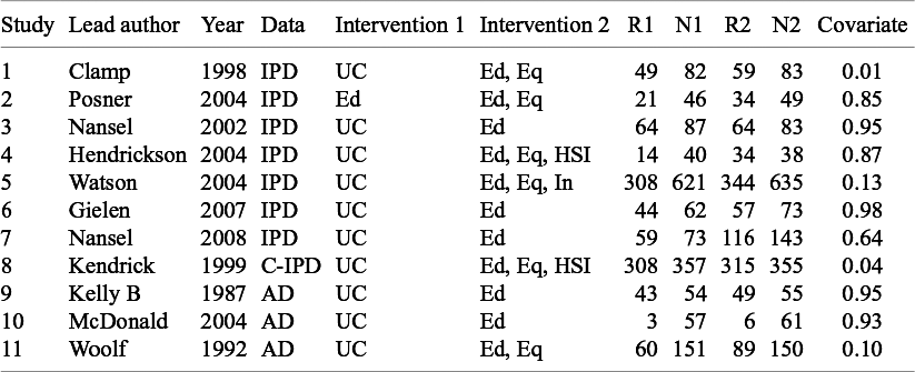
Table 1 summarises the original dataset for the outcome of safe storage of cleaning products used in this article. Data were available from 11 studies, including 3,355 participants. The table also shows the type of data available for each study in the dataset, including seven (64%) studies with IPD available, one (9%) cluster randomised study with IPD available, and three (27%) studies with only aggregate data available. IPD and cluster-IPD provide the binary outcome status for each participant (safely stored cleaning products or not after receiving the intervention), and the aggregate data provide the number of participants who achieved the outcome status in each study arm. Table 1 also presents the number of participants that safely stored cleaning products and the total number of participants in each trial arm. The covariate used in this analysis is the proportion of participants from ethnic groups other than the reference category (white ethnicity), which ranges from 0.01 to 0.98. We acknowledge that this broad categorisation does not follow ideal equity/equality, diversity, and inclusion (EDI) guidance. However, it reflects the motivating dataset and illustrates how the proposed methods can be used to address equity considerations by enabling the estimation of intervention effects within participant subgroups, which would not be possible using aggregate data only. We discuss the implications of this covariate choice and the associated EDI considerations further in Section 5.
Summary data from studies assessing interventions for promoting the safe storage of cleaning products to prevent childhood poisonings

Table 1 Long description
The table consists of 11 columns: Study, Lead author, Year, Data, Intervention 1, Intervention 2, R 1, N 1, R 2, N 2, and Covariate.
* Study 1: Clamp, 1998, I P D, U C, Ed and Eq, R 1 is 49, N 1 is 82, R 2 is 59, N 2 is 83, Covariate 0.01.
* Study 2: Posner, 2004, I P D, Ed, Ed and Eq, R 1 is 21, N 1 is 46, R 2 is 34, N 2 is 49, Covariate 0.85.
* Study 3: Nansel, 2002, I P D, U C, Ed, R 1 is 64, N 1 is 87, R 2 is 64, N 2 is 83, Covariate 0.95.
* Study 4: Hendrickson, 2004, I P D, U C, Ed and Eq and H S I, R 1 is 14, N 1 is 40, R 2 is 34, N 2 is 38, Covariate 0.87.
* Study 5: Watson, 2004, I P D, U C, Ed and Eq and In, R 1 is 308, N 1 is 621, R 2 is 344, N 2 is 635, Covariate 0.13.
* Study 6: Gielen, 2007, I P D, U C, Ed, R 1 is 44, N 1 is 62, R 2 is 57, N 2 is 73, Covariate 0.98.
* Study 7: Nansel, 2008, I P D, U C, Ed, R 1 is 59, N 1 is 73, R 2 is 116, N 2 is 143, Covariate 0.64.
* Study 8: Kendrick, 1999, C minus I P D, U C, Ed and Eq and H S I, R 1 is 308, N 1 is 357, R 2 is 315, N 2 is 355, Covariate 0.04.
* Study 9: Kelly B, 1987, A D, U C, Ed, R 1 is 43, N 1 is 54, R 2 is 49, N 2 is 55, Covariate 0.95.
* Study 10: McDonald, 2004, A D, U C, Ed, R 1 is 3, N 1 is 57, R 2 is 6, N 2 is 61, Covariate 0.93.
* Study 11: Woolf, 1992, A D, U C, Ed and Eq, R 1 is 60, N 1 is 151, R 2 is 89, N 2 is 150, Covariate 0.10.
Abbreviations: I P D is individual participant data, C minus I P D is clustered I P D, A D is aggregate data, U C is usual care, Ed is education, Eq is equipment, H S I is home safety inspection, In is installation, R is number of safe storers, N is total participants, and covariate is the proportion of non-white participants.
Note: IPD: individual participant data, C-IPD: clustered IPD, AD: aggregate data, UC: usual care, Ed: education, Eq: free or low-cost equipment, HSI: home safety inspection, In: installation of safety equipment, R: number of participants in study arm that safely stored their cleaning products, N: total number of participants in study arm, and covariate: the proportion of participants from ethnic groups other than the reference category (white ethnicity).
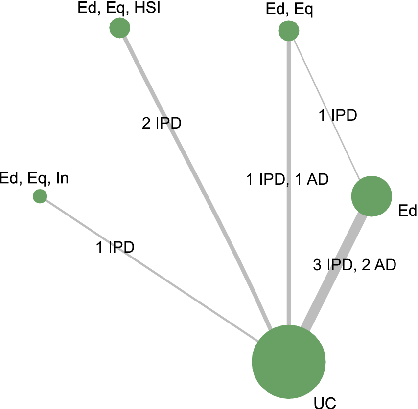
Figure 1 presents the network structure in terms of the study evidence available for each intervention comparison. The network consisted of six interventions that were made up of five components: usual care (UC), education, free or low-cost equipment, home safety inspection, and installation of safety equipment. Most studies compared interventions with UC; however, two studies included direct head-to-head comparisons between interventions.
Network plot of studies assessing interventions for promoting the safe storage of cleaning products to prevent childhood poisonings.
Note: IPD: individual participant data, AD: aggregate data, UC: usual care, Ed: education, Eq: free or low-cost equipment, HSI: home safety inspection, and In: installation of safety equipment.

Figure 1 Long description
A network plot with green circular nodes of varying sizes connected by gray lines of varying thicknesses.
* The largest node at the bottom is labeled U C.
* Moving clockwise from the far left, a small node labeled Ed, Eq, In is connected to U C by a thin line labeled 1 I P D.
* At the top left, a medium-small node labeled Ed, Eq, H S I is connected to U C by a medium-thickness line labeled 2 I P D.
* At the top center, a medium-small node labeled Ed, Eq is connected to U C by a medium-thickness line labeled 1 I P D, 1 A D. This node also has a very thin line labeled 1 I P D connecting it to the Ed node on the right.
* On the right, a medium-large node labeled Ed is connected to the U C anchor by the thickest line in the plot, labeled 3 I P D, 2 A D.
3. Methods
In this section, we describe Bayesian CNMA methods for synthesising evidence of complex interventions. The models described here use the generalised linear modelling framework for NMA models from the NICE Technical Support Document 2, which includes adjustments for multiarm trials and allows different choices of link functions for various outcome measures.Reference Dias, Welton, Sutton and Ades 28 We start by describing the CNMA models by Welton et al.Reference Welton, Caldwell, Adamopoulos and Vedhara 2 and Freeman et al.Reference Freeman, Scott, Powell, Johnston, Sutton and Cooper 25 for synthesising aggregate data, with and without covariate adjustment, followed by the novel CNMA models, including IPD, cluster-IPD, and aggregate data simultaneously, with and without covariate adjustment. The models use arm-based parametrisation and focus on binary outcomes, as this is relevant for the motivating example.
3.1. Model A: CNMA of aggregate data
We start by describing the CNMA model by Welton et al.Reference Welton, Caldwell, Adamopoulos and Vedhara
2
For studies where aggregate data are available, the number of participants that achieved the outcome in intervention j in study k,
$r_{jk}$
 , is assumed to follow a binomial distribution:

where
$n_{jk}$
 and
$p_{jk}$
 are the number of participants and the probability of the outcome in each study arm, respectively. The
$logit$
 link function transforms the probabilities to take values on the linear predictor scale, to enable additivity of intervention effects:

where
$\delta _{jk}$
 is the study-specific effect of intervention j compared to the intervention in the control arm of study k,
$b_k$
 . The indicator term,
$I_{{j\neq b_k}}$
 , is equal to 1 if
$j \neq b_k$
 , and equal to 0 if
$j=b_k$
 . Therefore, the
$\delta _{jk}$
 term is removed when estimating the effects of the study-specific control arm (denoted
$j=b_k$
 ) of each study and
$\mu _k$
 is the log-odds of an event in the control arm. The study-specific intervention random effects are assumed to follow a normal distribution with means equal to the difference in the underlying intervention effects (as defined by the consistency equations):

where
$d_{j}$
 is the underlying effect of intervention j compared to the reference intervention (denoted
$j=1$
 ) in the network (
$d_{1}=0$
 ) and
$\tau ^2$
 is the between-study heterogeneity. In the motivating example, the reference intervention is UC. Suppose that the interventions in the network are made up of
$nc$
 components,
$c_1,\ldots ,c_{nc}$
 . The additive main effects model assumes that the intervention effects are equal to the sum of the component effects within each intervention. In other words, the effect of intervention j compared to the network reference intervention
$j=1$
 is

where
$I_{j\ni c_{q}}$
 is equal to
$1$
 , if intervention j contains component q, and
$0$
 otherwise. Throughout this article, the reference intervention (denoted
$j=1$
 ) is UC, which we treat as an anchor component but only include the ‘active’ components in the count,
$nc$
 . Therefore, the component effects,
$d_{c_q}$
 , are the relative effects of component q versus UC and represent the effect of adding component q to UC. The component effects can be exchangeable, if there is clinical reasoning for this, but are modelled as independent throughout the rest of this article.
This additive model can also be extended to include terms for every pairwise combination of the components. This allows interventions with a particular pair of components to have synergistic or antagonistic effects (i.e., pairs of the components can have a larger or smaller effect than the sum of their effects). Additionally, inclusion of the full interaction effects would assume that every combination of components is independent and is equivalent to an NMA model.Reference Welton, Caldwell, Adamopoulos and Vedhara 2
3.2. Model B: CNMA of aggregate data with study-level covariate adjustment
CNMA was extended by Freeman et al. to include interactions between aggregate study-level covariates and intervention effectsReference Freeman, Scott, Powell, Johnston, Sutton and Cooper 25 :

where
$X_k$
 is the study-specific aggregated covariate and
$\beta ^B_{j}$
 are the covariate–intervention interactions. A random intervention effects model assumes that
$\delta _{jk} \sim N((d_{j}-d_{b_{k}}), \tau ^2)$
 and the underlying intervention effects are defined analogously to Equation (3.4) as the sum of component effects at the baseline covariate value and can be extended to include component interactions. In the same way that the intervention effects can be modelled in terms of their component effects, the covariate–intervention interactions can also be modelled in this way. For interventions made up of
$nc$
 components, the covariate–intervention interactions are assumed to be the sum of the covariate–component interaction effects,
$b_{1q}$
 for
$q=1,\ldots ,nc$
 , within each intervention:

The covariate–component interaction regression coefficients can be expressed as common, exchangeable, or independent. However, assuming the covariate–component interaction to be common would impose an assumption that as the number of components in the interventions increases, the effect of the covariate increases (e.g., if the covariate–component effects are common and
$b^W_{c_{q}}=b$
 where
$q=1,\ldots ,nc$
 , the component–intervention interactions would be equal to
$\beta ^W_{j}=nc_j \times b$
 ). This means that the covariate–component interactions will moderate the relative effects for interventions with differing numbers of components. For the motivating example in this article, they are assumed to be exchangeable. Alternatively, covariate–intervention interactions can be assumed to be independent, but the number of parameters is likely to restrict its applicability in practice.
3.3. Model C: CNMA of IPD and aggregate data
The following models were extended from Saramago et al.Reference Saramago, Sutton, Cooper and Manca 22 by defining the intervention effects and the covariate–intervention interactions in terms of their component effects, similar to the CNMA model by Welton et al. (Model A).Reference Welton, Caldwell, Adamopoulos and Vedhara 2 The model is structured in five parts. Parts 1–3 incorporate three types of data: individually allocated IPD, cluster-allocated IPD, and aggregate data. Part 4 combines the estimates of the first three parts using a shared parameter framework and Part 5 defines the component effects. This section presents the model without the inclusion of covariates.
3.3.1. Part 1: Model for IPD of individually allocated studies
Let the binary outcome for each participant, i, of each individually allocated study,
$Y_{ijk}$
 , come from a Bernoulli distribution with the probability of the event occurring
$p_{ijk}$
 :

The log-odds of an event are modelled by the following equation:

In the above equation,
$\mu ^{IPD}_{k}$
 is the log-odds of an event in the control arm of study k, denoted
$b_k$
 .
$\delta _{jk}$
 is the study-specific log-odds ratio comparing intervention j to the intervention in the control arm of study k.
$I_{j \neq b_k}$
 represents the intervention indicator, which equals
$0$
 for participants in the control arm,
$b_k$
 , and
$1$
 for participants in intervention arms.
3.3.2. Part 2: Model for IPD of cluster-allocated IPD studies
Let the binary outcome for participants in each cluster (denoted m) of the cluster-allocated studies,
$Y_{imjk}$
 , come from a Bernoulli distribution with the probability of the event occurring
$p_{imjk}$
 :

The log-odds of the event are modelled by

where
$\mu ^{c.IPD}_{mk}$
 is the log-odds of an event in the
$m^{th}$
 cluster of the control arm (
$b_k$
 ) of cluster-allocated study k, which are assumed to be exchangeable across clusters for each study, with mean
$\theta _k$
 and variance
$\tau .c_{k}^2$
 :

3.3.3. Part 3: Model for aggregate data studies
For studies where only aggregate data are available, the likelihood is modelled equivalently to Equation (3.1). This model and the following models throughout this article assume that the cluster-allocated studies that only have aggregate data available have made pre-model data adjustments to appropriately adjust for the clustering.
The log-odds are modelled as in Equation (3.2):

where
$\mu ^{AD}_k$
 is the log-odds of an event in the control arm of study k.
3.3.4. Part 4: Shared parameters across data types
The intervention effects are assumed to be exchangeable using a normal distribution across the IPD and aggregate data, with mean values that follow from the consistency assumptions as the difference in the basic parameters,
$d_j$
 :

where
$\tau ^2$
 is the between-study heterogeneity in the intervention effects.
3.3.5. Part 5: Defining component effects
Part 5 of the model defines the underlying intervention effects,
$d_{j}$
 , in Equation (3.13) in terms of their component effects relative to UC, as in Equation (3.4). Given there are
$nc$
 components and assuming an additive main component effects model:

where
$I_{j\ni c_{q}}$
 is an indicator variable that equals 1 when intervention j contains the component
$c_{q}$
 , for
$q=1,\ldots ,nc$
 , and is equal to 0 otherwise.
3.4. Model D: CNMA of IPD and aggregate data with study-level covariate adjustment
In this model, Parts 1 and 2 adjust for a study-level covariate by including a between-study interaction. Part 3 models the aggregate data and study-level covariate–intervention interaction analogously to Model B.
3.4.1. Part 1: Model for IPD of individually allocated IPD studies
For studies where IPD are available, the likelihood is equivalent to Equation (3.7) in Model C. However, the linear predictor includes two additional terms to incorporate the covariate:

In the above equation,
$\mu ^{IPD}_{k}$
 is the log-odds of an event in the control arm of study k at the baseline covariate value,
$x_{ik}$
 is the covariate value for individual i in study k, and
$\bar {x}_k$
 is the mean covariate value in study k.
$\delta _{jk}$
 is the study-specific log-odds ratio comparing intervention j to the intervention in the control arm of study k, denoted
$b_k$
 .
$\beta ^0_{k}$
 denotes the study-specific individual-level additive effect of a unit increase in the covariate,
$x_{ik}$
 , on the log-odds of the event in the control arm of study k.
$\beta ^B_{jk}$
 models the between-study covariate–intervention interaction.
$I_{j \neq b_k}$
 represents the intervention indicator, which equals
$0$
 for participants in the control arm, and
$1$
 for participants in the intervention arms.
3.4.2. Part 2: Model for IPD of cluster-allocated studies
For studies where IPD are available for cluster-allocated studies, the likelihoods are modelled equivalently to Equation (3.9) in Model C. However, as in Part 1, two additional terms in the linear predictor incorporate the covariate:

where
$\mu ^{c.IPD}_{k}$
 is the log-odds of an event in the control arm of cluster-allocated study k at the baseline covariate value,
$x_{imk}$
 is the covariate value for individual i in cluster m of study
$k,$
 and
$\bar {x}_k$
 is the mean covariate value in study k. The control arm log-odds are assumed to be exchangeable across clusters, as in Equation (3.11).
3.4.3. Part 3: Model for aggregate data studies
For studies where only aggregate data are available, the likelihood is equivalent to Equation (3.1).
The log-odds are modelled as

where
$\mu ^{AD}_k$
 is the log-odds of an event in the control arm of study k at the baseline covariate value.
$X_k$
 is the study-specific aggregated covariate value in study k.
3.4.4. Part 4: Shared parameters across data types
The intervention effects are assumed to be exchangeable using a normal distribution across the IPD and aggregate data, with mean values that follow the consistency assumptions as the difference in the basic parameters:

where
$\tau ^2$
 is the between-study heterogeneity in the intervention effects.
3.4.5. Part 5: Defining component effects
Part 5 of the model defines the intervention effects and between-study covariate–intervention interaction effects,
$d_{j}$
 and
$\beta ^B_{j}$
 , in Equation (3.18) in terms of their component effects. Given there are
$nc$
 components and assuming an additive main component effects model:


where
$I_{j\ni c_{q}}$
 is an indicator variable that equals 1 when the intervention j contains the component
$c_{q}$
 , for
$q=1,\ldots ,nc$
 , and is equal to 0 otherwise.
$d_{c_{q}}$
 are the component effects at the baseline covariate value and
$b^B_{c_{q}}$
 are the between-study covariate–component interactions. The covariate–component interactions are assumed to be exchangeable throughout this article.
3.5. Model E: CNMA of IPD and aggregate data with individual-level and study-level covariate adjustment
This model includes covariate adjustment with the separation of individual- and study-level covariate–intervention interactions to address aggregation bias. Parts 1 and 2 model the IPD, which can capture the within-study covariate–intervention interactions as well as the between-study covariate–intervention interactions, by partitioning the variability of the covariate–intervention interactions into the two estimates, as originally proposed by Riley and Steyerberg.Reference Riley and Steyerberg 29 Part 3, which models the aggregate data, can only inform the estimation of the between-study covariate–intervention interactions.
3.5.1. Part 1: Model for IPD of individually allocated studies
For studies where IPD are available, the likelihood is modelled equivalent to Equation (3.7) in Model D. However, to extend Model C, a within-study covariate–intervention interaction term is included:

In the above equation,
$\beta ^W_{j}$
 models the within-study covariate–intervention interaction and
$\beta ^B_{j}$
 models the between-study covariate–intervention interaction. The within-study association is modelled by centring the individual covariate,
$x_{ik}$
 , about the study mean covariate value,
$\bar {x}_k$
 . All other parameters are defined as in Model D.
3.5.2. Part 2: Model for IPD of cluster-allocated studies
For studies where IPD are available for cluster-allocated studies, the likelihoods are modelled equivalently to Equation (3.9) in Model C. However, as in Part 1, an additional term in the linear predictor incorporates the within-study covariate–intervention interaction:

where, as in Part 1, within-study association,
$\beta ^W_{j}$
 , is modelled by centring the individual covariate,
$x_{ik}$
 , about the study mean covariate value,
$\bar {x}_k$
 . The control arm log-odds are assumed to be exchangeable across clusters, as in Equation (3.11). All other parameters are defined as in Model D.
3.5.3. Part 3: Model for aggregate data studies
For studies where only aggregate data are available, the likelihood is equivalent to Equation (3.1). Aggregate data in this form cannot inform within-study association. Therefore, the log-odds are modelled equivalently to Model D with equivalent parameter definitions but are repeated here for completeness:

3.5.4. Part 4: Shared parameters across data types
The intervention effects and covariate–intervention interaction effects are assumed to be exchangeable using a normal distribution across the IPD and aggregated data, with mean values that follow the consistency assumptions as the differences in the basic parameters:

where
$\tau ^2$
 is the between-study heterogeneity in the intervention effects.
3.5.5. Part 5: Defining component effects
Part 5 of the model defines
$d_{j}$
 ,
$\beta ^B_{j}$
 , and
$\beta ^W_{j}$
 , in Equation (3.24), for each intervention j in terms of their component effects. Given there are
$nc$
 components across all interventions and assuming an additive main component effects model:


where
$I_{j\ni c_{q}}$
 is an indicator variable that equals 1 when the intervention j contains the component
$c_{q}$
 and is equal to 0 otherwise.
$d_{c_{q}}$
 are the component effects at the baseline covariate,
$b^B_{c_{q}}$
 are the between-study covariate–component interactions, and
$b^W_{c_{q}}$
 are the individual-level (within-study) covariate–component interactions. The aggregation bias at the component level can be assessed by calculating the posterior distributions of
$b_{diff,c_q}=b^B_{c_{q}}-b^W_{c_{q}}$
 for each component
$c_q$
 . If there is no evidence of aggregation bias, then the individual,
$b^W_{c_{q}}$
 , and study-level covariate–component interactions,
$b^B_{c_{q}}$
 , are similar and can be combined in the first two parts of this model, which can improve the power to estimate the interactions.
3.6. Implementation and software
All of the models were fitted in WinBUGS 1.4.3 through the R package, R2WinBUGS.Reference Spiegelhalter, Thomas, Best and Lunn 30 , Reference Sturtz, Ligges and Gelman 31 The WinBUGS code used for Models D and E is available at https://github.com/elleshasmith/winbugs-code-ipd-cnma.git. Posterior estimates were based on 50,000 burn-in and 50,000 sample iterations, and vague prior distributions were used and checked for sensitivity to initial values and prior distributions. Details on the prior distributions and initial values used to run the models can be found in Appendix A of the Supplementary Material. Autocorrelation plots, history, and density plots were visually assessed to identify signs of non-convergence. The network plot (Figure 1) was created using the BUGSnet package in R.Reference Béliveau, Boyne, Slater, Brenner and Arora 32
4. Results
The results of applying the methods described to the Keeping Children Safe dataset for the safe storage of cleaning products to prevent childhood poisonings outcome are presented in Figure 2 for the component combination effects and Figure 3 for the covariate–intervention interaction effects. All of the results are reported as odds ratios (OR) with their corresponding 95% credible intervals (CrIs), relative to the reference intervention UC. There was no evidence of non-convergence, although autocorrelation was high for some parameters (Appendix B of the Supplementary Material). However, sensitivity analyses showed that conclusions were robust to increasing the sample length, the choice of initial values, and prior distributions (example results in Appendix C of the Supplementary Material).
Results of applying the five models to the motivating example for the component combination effects relative to usual care, reported as odds ratios and their relative 95% credible intervals. Notation: IPD: individual participant data, AD: aggregate data, UC: usual care, Ed: education, Eq: free or low-cost equipment, HSI: home safety inspection, In: installation of safety equipment, ILA: individual-level adjustment, and SLA: study-level adjustment.

Figure 2 Long description
The X-axis represents the Log odds ratio and 95 percent credible interval (truncated at minus 5), ranging from minus 5 to 5 with a vertical dashed red line at 0. The Y-axis lists 15 component combinations from top to bottom: Ed; Eq; H S I; In; Ed, Eq; Ed, H S I; Ed, In; Eq, H S I; Eq, In; H S I, In; Ed, Eq, H S I; Ed, Eq, In; Ed, H S I, In; Eq, H S I, In; and Ed, Eq, H S I, In.
Each category contains five colored dots with horizontal whiskers representing different models:
- Model A: C N M A (purple)
- Model B: C N M A S L A (blue)
- Model C: C N M A with I P D (green)
- Model D: C N M A with I P D S L A (olive)
- Model E: C N M A with I P D S L A and I L A (red)
General trends show that Model A (purple) and Model B (blue) often have wider credible intervals compared to models incorporating I P D (C, D, and E). Most estimates cluster around the null line (0), though combinations involving Ed and Eq tend to shift slightly positive, while single components like In show slightly negative log odds ratios across all models.
Covariate–intervention interaction results for Models B, D, and E. Notation: IPD: individual participant data, AD: aggregate data, UC: usual care, Ed: education, Eq: free or low-cost equipment, HSI: home safety inspection, In: installation of safety equipment, ILA: individual-level adjustment, and SLA: study-level adjustment.

Figure 3 Long description
A multi-panel figure consisting of two forest plots, labeled a and b.
Panel a, titled Between-study covariate-intervention interaction estimates, relative to usual care. The x-axis represents the Log odds ratio and 95 percent credible interval, ranging from minus 5 to 5, with a vertical dashed line at 0. The y-axis lists 14 component combinations: Ed; Eq; H S I; In; Ed, Eq; Ed, H S I; Ed, In; Eq, H S I; Eq, In; H S I, In; Ed, Eq, H S I; Ed, Eq, In; Ed, H S I, In; Eq, H S I, In; and Ed, Eq, H S I, In. A legend identifies three models: Model B (C N M A S L A) in blue, Model D (C N M A with I P D S L A) in green, and Model E (C N M A with I P D S L A and I L A) in red. For each y-axis category, three horizontal lines with central dots represent the estimates. Most estimates for Model B are positive (right of 0), while Models D and E show more variability, often centered closer to 0 or negative for single components like Ed and In, but becoming more positive for complex combinations like Ed, Eq, H S I, In.
Panel b, titled Within-study covariate-intervention interaction estimates, relative to usual care. It uses the same x-axis and y-axis categories as panel a. The legend identifies only Model E (C N M A with I P D S L A and I L A) in red. The data points and error bars are generally centered closer to the 0 line compared to panel a, with wider credible intervals. Single components like Ed and H S I show negative log odds ratios, while combinations like Eq, In and Eq, H S I, In show positive log odds ratios.
Additivity was assessed by comparing model fit using the deviance information criterion (DIC) between a standard NMA model and the additive CNMA model.Reference Rücker, Petropoulou and Schwarzer 3 , Reference Veroniki, Wolfe and Hutton 33 The additive CNMA model yielded a slightly lower DIC compared with a standard NMA model, indicating a similar fit to the observed data (Appendix D of the Supplementary Material). The small difference in DIC (approximately 1.4) suggests that the assumption of additivity does not compromise model fit and is therefore likely to be reasonable in this analysis.
4.1. Models without covariates (Models A and C)
For Model A, there was little evidence that the individual components or combinations of components are effective at improving the safe storage of cleaning products. There was evidence that the education, equipment, and home safety inspection (Ed, Eq, HSI) component combination was effective at promoting the safe storage of cleaning products, compared to UC, with an odds ratio of 3.28 (95% CrI: 0.98, 15.29) but the CrI crosses the point of no effect.
Including IPD in the CNMA model (Model C), for studies where it was available, produced similar median posterior effect estimates to the aggregate data results but slightly reduced the widths of the CrIs for the component and component combination effect estimates. The CrI of the effect estimate for the education, equipment, and home safety inspection (Ed, Eq, HSI) component combination no longer crossed the point of no effect (OR: 3.35, 95% CrI: 1.00, 15.18), providing improved evidence that this combination is effective at promoting the safe storage of cleaning products, compared to UC.
Including the available IPD marginally reduced the between-study variance from 0.51 (95% CrI: 0.05, 2.88) in Model A to 0.49 (95% CrI: 0.05, 2.94) in Model C, but the uncertainty in this estimate slightly increased.
4.2. Methods with covariate adjustment (Models B, D, and E)
After including the ethnicity covariate in the CNMA model as aggregate outcome and covariate data (Model B), the education, equipment, and home safety inspection (Ed, Eq, HSI) component combination effect estimate showed no evidence of promoting the safe storage of cleaning products, compared to UC, in the baseline covariate group (in a white population). However, there was evidence of a covariate interaction with this component combination (OR: 16.83, 95% CrI: 2.96, 123.70, Figure 3). This interaction estimate implies that for every 10% increase in the proportion of individuals from ethnic groups other than the reference category (white ethnicity) in a study population, the odds ratio comparing the safe storage of cleaning products in the education, equipment, and home safety inspection (Ed, Eq, HSI) component combination, relative to UC, increases by 32%.Footnote 1 Compared to models without covariate adjustment, the between-study heterogeneity of the intervention effects reduced to 0.04 (95% CrI: 0.00, 0.97) and the uncertainty in the estimate also improved. However, the between-study heterogeneity of the covariate–component interactions was high and very uncertain, estimated as 4.65 (95% CrI: 0.01, 81.28).
The inclusion of the available IPD into the study-level adjustment model (Model D) increased the uncertainty of the effect estimates and there was little evidence that the individual components or combinations of components are effective at improving the safe storage of cleaning products in the baseline covariate group (in a white population). There was also little evidence of covariate–component interaction effects. Additionally, the between-study heterogeneity was larger than for the model including the covariate as aggregate data at 0.17 (95% CrI: 0.00, 2.37). However, the inclusion of IPD reduced the between-study heterogeneity of the covariate–component interactions, estimated as 1.46 (95% CrI: 0.14, 6.63).
Model E results demonstrated no evidence that individual components or combinations of components are effective at improving the safe storage of cleaning products in the baseline covariate group (in a white population). There was also no evidence of individual-level covariate–component combination interactions. However, notice that, at the study level, there is evidence of an interaction between the covariate and the education, equipment, and home safety inspection (Ed, Eq, HSI) component combination, with the odds ratio estimated as 19.57 (95% CrI: 3.50, 138.70). This result implies that for every 10% increase in the study proportion of individuals from ethnic groups other than the reference category (white ethnicity) in a population, the odds ratio comparing the safe storage of cleaning products in the education, equipment, and home safety inspection (Ed, Eq, HSI) component combination, relative to UC, increases by 35%.Footnote 2 However, this association should be interpreted with caution, as study-level covariates are susceptible to confounding by other between-study differences. The between-study heterogeneity of the intervention effects was estimated to be 0.03 (95% CrI: 0.00, 0.72) and heterogeneity parameters for the within- and between-study covariate–component interactions were 1.85 (95% CrI: 0.07, 8.60) and 1.88 (95% CrI: 0.01, 47.71), respectively.
5. Discussion
In this article, we develop CNMA methods that incorporate IPD, where it is available, and aggregate data, where IPD is not available, to evaluate the effectiveness of components and combinations of components within complex interventions. We also extend the models to adjust for individual-level covariates, by separating out the within-study and between-study interaction effects to address aggregation bias. The methods were applied to a dataset of 11 studies, of which eight had IPD available, from a Cochrane systematic review evaluating the effectiveness of complex home safety practices for promoting the safe storage of cleaning products to prevent childhood poisonings.
In comparison to previous literature, the models presented here are designed to simultaneously combine the multiple data types to maximise use of all available evidence, while addressing aggregation bias in the covariate–intervention interactions. Efthimiou et al. focused on component interaction selection methods but do not address aggregation bias or separate out individual- and study-level estimates. In addition, this article explicitly defines a binary outcome model, detailing the likelihood and link function and separately synthesises IPD of cluster-allocated RCTs to adjust for similarity of individuals within clusters.
5.1. Strengths and limitations
The additivity assumption of CNMA models facilitates the estimation of the effects of components and combinations of components that are within the connected network of evidence. Application of the CNMA models presented in this article to the motivating example demonstrates this beneficial feature, since the effects of all combinations of the home safety practices are reported, rather than only the combinations in the direct study evidence. CNMA methodology has the potential to reduce research waste by directing future research to combinations of intervention components that have the potential to be the most effective.
Although the additivity assumption is a useful characteristic of CNMA models, it is important in practice to assess whether this assumption is reasonable when the models are applied to real data. This assumption can be examined by comparing model fit statistics, such as the DIC and residual deviance, between the additive CNMA model and more flexible specifications that relax additivity (e.g., interaction models or NMA).Reference Rücker, Petropoulou and Schwarzer 3 In practice, interaction terms should be specified based on clinical or biological plausibility, focusing on combinations where synergistic or antagonistic effects are expected.Reference Veroniki, Wolfe and Hutton 33 It is generally recommended to include a limited number of pre-specified interactions and to assess their contribution to model fit. In our analysis, the DIC values were similar between the standard NMA and additive CNMA models, suggesting that the additivity assumption was not strongly violated. Evaluating this assumption in applied analyses helps to ensure the validity of the component and component combination effect estimates.
This article focused on binary outcomes, as appropriate for the motivating example. However, a key strength of the proposed methods is that they naturally extend to other types of data by utilising the generalised linear framework described in the NICE Technical Support Document 2. Replacing the binomial/Bernoulli distributions and logit links with an appropriate family of distributions and link function allows the models to be applied to other outcome types. This flexibility means that the models are readily applicable across diverse datasets and clinical areas.
The motivating example enabled the comparison of CNMA methods with aggregate data alone with methods including IPD for studies where it was available. For the models without adjustment for the covariate (Models A and C), the inclusion of IPD reduced the between-study heterogeneity and the size of the CrIs of the component-combination effects. This was also observed for estimates of the effects of study-level covariate–component combination interactions (Models B and D). The finding, that the inclusion of IPD can improve the precision of effect estimates, aligns with the existing literature, which describes this effect theoretically and demonstrates it through simulation and applied examples in various pairwise and NMA models.Reference Lambert, Sutton, Abrams and Jones 24 , Reference Leahy, O’Leary and Afdhal 34 – Reference Riley, Dias and Donegan 38
This article proposes a range of methods that demonstrate the benefits and limitations of the available methods in situations where a mixture of IPD and aggregate data are available. Prior to the development of methods that incorporate IPD, covariate–intervention interactions were often estimated using aggregate data alone (Model B). Whilst this method is appropriate for inclusion of study-level covariates, for individual-level covariates this method was found to be subject to aggregation bias. In the motivating example, this is demonstrated as Model B showed evidence of an interaction between ethnicity and effectiveness of the education, free equipment, and home safety installation. A common but incorrect interpretation of this effect would conclude that the intervention is more effective for individuals from ethnic groups other than the reference category (white ethnicity). The estimated effect could be the result of aggregation bias, due to confounding or effect modification. Models that incorporate IPD but only estimate the between-study covariate–intervention (Model D) are also subject to aggregation bias.Reference Fisher, Carpenter, Morris, Freeman and Tierney 39 Interpreting study-level interactions as individual-level ones could cause misleading conclusions that feed into healthcare decision making, resulting in inefficient allocation or waste of resources and worsening health inequities. The benefit of Model E is that it addresses aggregation bias by separating out the between-study and within-study interactions. Application of Model E to the motivating example demonstrated evidence of aggregation bias as there was no evidence of an interaction between ethnicity and the effectiveness of the education, free equipment, and home safety installation but there was evidence of an interaction at the study-level. The uncertainty in the effect estimates is high, indicating that there are currently not enough studies in this motivating example dataset to estimate individual-level interactions. However, this model has the potential to be extremely useful for decision making and healthcare allocation as it can identify covariates that affect the component combination effects and, therefore, identify which combinations of components have the potential to work best for which subgroups of individuals. These findings have the potential to guide future research studies, reduce health inequities, and reduce research waste.
NMA of IPD is considered the gold standard for evidence synthesis to inform healthcare decision making. However, the literature demonstrates how difficult it is to obtain IPD for every study identified from a review. A review from 2017 showed that this was not improving.Reference Nevitt, Marson, Davie, Reynolds, Williams and Smith 19 However, recent changes such as the requirement to provide data sharing or data availability statements in publications and new repositories for sharing data means that this may have changed since these reviews.Reference Taichman, Sahni and Pinborg 40 , Reference Jiao, Li and Fang 41 Despite this, a benefit of the models proposed in this article is that there is no requirement to obtain IPD for every study, as the studies without IPD are incorporated as aggregate data, which contributes to the between-study covariate–component interaction effect estimates and is an efficient use of all the available data.
Although the inclusion of IPD is often expected to increase precision, in some comparisons, we observed wider CrIs after incorporating IPD. This may reflect increased model complexity, as IPD models typically estimate additional parameters, leading to greater uncertainty. In addition, combining IPD with aggregate data may reveal heterogeneity or inconsistencies between the IPD and aggregate data, which can inflate posterior uncertainty. Finally, IPD models allow a more flexible representation of variability within and between studies, which can better capture heterogeneity and may result in wider, but more appropriate, CrIs.
The methods in this article were proposed in a Bayesian setting, which offers a flexible approach to model development, allows the inclusion of external information from previous studies or expert opinions through prior distributions, and the ability to obtain direct probability statements.Reference Spiegelhalter, Abrams and Myles 42 These characteristics are all beneficial in the context of decision making. However, the methods are statistically complex and the use of Bayesian implementation adds another dimension of complexity which could prove to be a major barrier to their future implementation.
When applying CNMA models, we followed the common approach of assigning independent priors to component effects. An implication of the additive structure of the CNMA models is that the prior variances for the multicomponent interventions increase with the number of components it contains. Since the variance of a sum of independent component effects is the sum of their variances, the models imply that multicomponent interventions have larger prior uncertainty, which can translate into wider posterior CrIs when data are sparse. This reflects the structural properties of the model rather than true differences in the underlying evidence base, which can hinder interpretation. Modelling options to mitigate this issue include scaling the prior variances by the number of components, re-parametrising the model so that the variance priors are placed on the intervention effects and the component effects are modelled as fixed-effect parameters, or introducing a multivariate normal prior distribution on the component effects with a correlation structure. Future work could explore these alternative models for variance priors to assess whether the increased model flexibility improves precision and interpretability.
Statistical methodology development should include an assessment for EDI if real-life datasets are used in its development or the methods may be applied to healthcare data in the future.Reference Smith, Akroyd and Barnes 43 As previously discussed, aggregation bias can exacerbate inequalities, when using inappropriate methodology (such as Models B and D) to draw conclusions about individual-level covariates, such as ethnicity, if the conclusions inform healthcare decision making or allocation of resources. Comparatively, Model E estimates both study-level and individual-level interaction effects, which addresses aggregation bias and, if applied appropriately, has the potential to identify which interventions work best for whom, therefore reducing health inequalities by drawing on personalised medicine principles. However, as the motivating example in this article has shown and previous paragraphs in this discussion highlight, there are characteristics of these models that need further investigation and application should be cautious, particularly when evidence is limited.
Regarding the motivating example, the purpose of the dataset and including ethnicity as a covariate was to demonstrate key characteristics of the models and highlight the implications of using these models in future evidence synthesis of health interventions. Considerations and recommendations for the use of ethnicity as quantitative variables in medical research is discussed in the literature, but the rationale for this decision in this article is solely illustrative.Reference Ross, Hart-Johnson, Santen and Zaidi 44 The use of this dataset and the results of the analyses are not meant to inform clinical decision making.
5.2. Further research
Future research could conduct a simulation study to investigate the impact of IPD on the estimates and assess the generalisability of the methods proposed in this article. Varying the level of IPD can help to assess what proportion is required to improve the precision of effect estimates for individual-level interactions. This additional information could be used to assess whether it is worth spending the additional time and effort obtaining IPD to improve estimation of intervention effects, particularly in sub-populations, before commissioning further research.
This manuscript focuses on the methodological development and applied analysis. To support transparency and reproducibility, the model code is provided on GitHub (https://github.com/elleshasmith/winbugs-code-ipd-cnma.git). However, an R package implementing these models would greatly improve accessibility. Developing such software is a priority for future work and would support wider adoption of these methods.
6. Conclusion
In this article, we propose CNMA methods that simultaneously synthesise the IPD, where it is available, with aggregate data, where IPD is not available. This approach addresses aggregation bias while allowing the incorporation of individual-level covariates and facilitates the estimation of covariate–component interaction effects at both the individual and study level, to provide more information to decision makers regarding which component combinations work best for whom. Due to the high number of parameters that are estimated by this model, the application of CNMA combining IPD and aggregated data may be most appropriate in settings where sufficient data are available. Further research is required to identify situations where application of CNMA including IPD and aggregated data could provide useful insights that meaningfully inform research design and healthcare decision making.
Acknowledgements
We thank the study team for their work on data collection and management, and Prof. Denise Kendrick, Chief Investigator, for permission to use the data.
Author contributions
Conceptualisation: E.A.S. and S.J.H.; Data curation: S.J.H.; Data visualisation: E.A.S.; Methodology: E.A.S., S.J.H., and S.C.F.; Supervision: L.J.G., S.J.H., S.C.F., and N.J.C.; Writing—original draft: E.A.S.; Writing—reviewing and editing: E.A.S., S.C.F., L.J.G., S.J.H., and N.J.C. All authors approved the final submitted draft.
Competing interest statement
E.A.S. was funded by the UK National Institute for Health and Care Research (NIHR) Doctoral Research Fellowship (Award No. DRF-2018-11-ST2-033). L.J.G. is funded by the National Institute for Health and Care Research (NIHR) Applied Research Collaboration East Midlands (ARC EM) and Leicester NIHR Biomedical Research Centre (BRC [NIHR203327]). L.J.G. is an NIHR Senior Investigator and a member of the NIHR Multiple Long-Term Conditions Cross-NIHR Collaboration. L.J.G. is supported by the British Heart Foundation Research Excellence Award (RE/24/130031). The views expressed are those of the authors and not necessarily those of the NIHR or the Department of Health and Social Care.
Data availability statement
This work uses anonymised individual participant data from the Keeping Children Safe at Home programme (Award ID: RP PG 0407 10231). The data underlying this study consist of individual participant data obtained from multiple independent studies. These data are not publicly available as they are owned by the original investigators and were shared with the authors under specific data sharing agreements and ethical approvals. Access to the data may be requested from the original data custodians. Requests for access can be directed to Prof. Denise Kendrick, University of Nottingham, who can advise on the appropriate process for contacting the relevant data contributors.
Funding statement
This study was supported/funded by the National Institute for Health and Care Research (NIHR) Applied Research Collaboration East Midlands (ARC EM) and Leicester NIHR Biomedical Research Centre (BRC).
Ethical standards
The research meets all ethical guidelines, including adherence to the legal requirements of the study country.
Supplementary material
The supplementary material for this article can be found at https://doi.org/10.1017/rsm.2026.10119.




 Open access

