


Dynamic models of elections have increasingly become an important focus of political economy and formal political science. An advantage of these models over static models is that they allow, in principle, the possibility of policy dynamics. They enable analysis of the interplay between dynamic incentives and information on the part of voters and politicians, and they permit the analysis of essentially dynamic issues such as incumbency advantage, the consequences of term limits, and the effects of re-election incentives on policy choices. And to the extent that equilibrium policies resemble the ideal policy of the median voter, these models can provide non-cooperative underpinnings for the classical median voter theorem. This article considers a framework for repeated elections, analyzed in Duggan (Reference Duggan2000), in which politicians’ preferences are private information, and voters update their prior beliefs about an office holder's type on the basis of her past policy choices; thus the model is one of pure adverse selection. In equilibrium, therefore, an office holder's policy choice reflects her short-term preference to implement desirable policy for the current period and long-term considerations of the impact on her chances for re-election; and each voter compares a relatively familiar incumbent with the prospect of an untried challenger.
The subject of analysis has naturally been on equilibria that have a stationary structure: the policy choice of a politician is a constant function of her type, and voters condition only on an office holder's current policy choice. This structure often implies that equilibria have a partitional form, with centrist politicians choosing their ideal policies and being re-elected, extremist politicians choosing their ideal policies and being removed from office, and moderate politicians pooling at a policy close to the median in order to gain re-election. The analysis of these equilibria reveals the possibility of incumbency advantage, as voter risk aversion creates some scope for a centrist politician to gain re-election by choosing a policy close (but not equal) to the median, and moderate politicians compromise in order to gain re-election. Banks and Duggan (Reference Banks and Duggan2008) show that when citizens (voters and politicians) become arbitrarily patient, politicians almost always compromise by choosing policies arbitrarily close to the median ideal policy, delivering a version of the median voter theorem based on a model of dynamic elections with private information. Adding a term limit, an office holder simply chooses her ideal policy in her last term of office, and the partition in general depends on the incumbent's tenure in office. See Duggan (Reference Duggan2000) and Banks and Duggan (Reference Banks and Duggan2008) for analysis of the model without term limits, and see Bernhardt et al. (Reference Bernhardt, Dubey and Hughson2004) for the model with term limits. Further applications include the analysis of public goods with privately observed budget constraints (Meirowitz (Reference Meirowitz2007)), parties (Bernhardt et al. (Reference Bernhardt, Campuzano, Squintani and Camara2009)), valence (Bernhardt, Camara and Squintani (Reference Bernhardt, Camara and Squintani2011)) and taxation (Camara (Reference Camaro2012)).Footnote 1
Although the focus on stationary equilibria is a natural starting point, and can be viewed as an identifying assumption to generate testable implications of the model, it is important from a theoretical perspective to understand the restrictions on behavior implicit in this refinement. To this end, I formulate a more permissive equilibrium concept, called ‘perfect Bayesian electoral equilibrium,’ which allows politicians and voters to condition on past policy and election outcomes. I establish a folk theorem for the electoral model: when politicians and voters are sufficiently patient, arbitrary paths through an arbitrarily large region of the policy space can be supported as outcomes of perfect Bayesian electoral equilibria. In fact, the theorem extends to support any incentive-compatible assignment of policy paths to types. The results do not follow from extant results on the folk theorem in the context of repeated games. For one reason, the game is not a repeated game, as voters alternate moves with politicians, and the identity of the office holder may change over time. More importantly, a politician's type is private information, so voters and future politicians cannot condition their choices on the current office holder's type; thus, the equilibrium concept must specify beliefs as well as strategies, and the appropriate concept should be consistent with the spirit of perfect Bayesian equilibrium. In fact, among other things, the refinement I propose excludes the possibility of targeting individual voters for their votes, and it imposes a stage-game dominance condition on voting strategies, so a voter votes for the incumbent if the expected discounted payoff from re-electing the incumbent is at least equal to that from electing an untried challenger.
Several more comments on the strength of this result are in order.
• I assume politicians are purely policy motivated. This assumption means that a politician cannot be punished simply by removing her from office, and it significantly complicates the problem of incentivizing desired policy choices.
• I assume the policy space is the unit interval. This assumption precludes the use of punishments involving arbitrarily bad policy choices, and it restricts the dimensionality of the space of payoff imputations and precludes the possibility of targeting punishments to particular office holder types––even if the politicians’ types were observed.
• Reinforcing the latter remark, because voters cannot observe the type of an office holder, punishment strategies in principle cannot be type specific—so they must ‘thread the needle’ by responding to deviations in a way that avoids rewarding one type while punishing another.
• Nevertheless, the folk theorem establishes that arbitrary policy paths can be supported in a strong sense: in each period, all types of office holders choose the same pre-specified policy.
• I do not exploit impatience of politicians by using an initial finite number of periods to elicit an office holder's type; instead, I construct equilibria that generate arbitrary histories from the beginning of the game.
The equilibrium construction is delicate. For a policy path that takes a constant value near one extreme of the policy space, the construction must induce an office holder from the other side of the ideological spectrum to choose that policy (which is arbitrarily close to the worst possible) over an infinite horizon. And paths that are not constant are supported by punishments that ‘splice’ these extremal equilibria together and alternate between the two extremes with appropriate frequency. The construction relies critically on differentiability of politician utility functions to address the former issue, and on strict concavity of utilities to address the second, in contrast to other folk theorem results that do not require such fine structure.
The conclusion of the analysis is that the restriction to stationary equilibria in existing work on models of repeated elections with adverse selection is substantial—and necessary for generating empirically meaningful predictions—for without some limitation on the extent of conditioning on histories (or an a priori bound on the rate of discount), almost any policy path is consistent with equilibrium. This is reminiscent of the cycling results of Plott (Reference Plott1967), McKelvey (Reference McKelvey1976, Reference McKelvey1979), and Schofield (Reference Schofield1978, Reference Schofield1983) in the multidimensional model with an empty majority core, but the current analysis holds in one dimension, and it is based on a non-cooperative equilibrium analysis that explicitly addresses the strategic incentives of politicians and voters. Closest to the current article is Duggan and Fey (Reference Duggan and Fey2006), who analyze repeated Downsian elections, in which two office-motivated parties compete in an infinite sequence of elections. In each period, the two parties simultaneously announce policy platforms, and the winning party is bound to its promise. That article considers the general multidimensional model, and Theorem 1 of the article establishes that when voters are relatively patient (discount factors greater than one-half), every policy path can be generated by a subgame perfect equilibrium. Whereas the latter result holds generally, Duggan and Fey's (2006) Theorem 2 applies when the majority core is nonempty and is perhaps most comparable to the folk theorem of this article: it establishes that when parties are relatively patient (and voters’ discount factors are positive), every policy path is generated by a subgame perfect equilibrium.
Of course, folk theorems have been proved for abstract dynamic games. Fudenberg and Maskin (Reference Fudenberg and Maskin1986) state the folk theorem for subgame perfect equilibria of discounted repeated games, and this is extended to repeated games with imperfect public monitoring by Fudenberg, Levine and Maskin (Reference Fudenberg, Levine and Maskin1994). Because voters and office holders alternate moves, however, the repeated elections model is not the simple repetition of a fixed-stage game. Wen (Reference Wen2002) proves a folk theorem in repeated ‘sequential games,’ which assumes that in each period, players play an extensive form game such that players are partitioned into groups, groups move sequentially, players within a group choose simultaneously and their feasible action sets are independent of others’ choices. The timing of moves in this framework has some similarity to the electoral model, with an office holder first choosing policy and then voters simultaneously casting ballots, but it differs in the respect that the electoral model assumes a countably infinite set of candidates, and the identity of the office holder can conceivably change every period. Dutta (Reference Dutta1995) establishes a folk theorem for stochastic games, which generalize sequential games, and Horner et al. (Reference Horner, Sugaya, Takahashi and Vieille2011) and Fudenberg and Yamamoto (Reference Fudenberg and Yamamoto2011) extend the result to games with imperfect public monitoring, but again this work assumes a finite number of players. In addition, the above articles assume finite action sets, whereas the electoral model allows office holders to choose from a convex policy space. More importantly, the above articles assume that payoff functions are complete information, precluding the possibility of adverse selection and the difficult problems it entails.Footnote 2
As perfect Bayesian electoral equilibria refine the standard concept of perfect Bayesian equilibrium, it stands that voter beliefs are updated via Bayes’ rule along the path of play, and the construction I describe in fact delivers more: even off the path of play from the initial history, voter beliefs about the type of a challenger are given by a fixed, common prior, and voters apply Bayes’ rule separately along the personal path of play of every office holder. And along the path of play from the initial history, all politician types choose the same policy (which may vary across periods), the first office holder is re-elected in every period, and voters do not revise their beliefs. But I do exploit some flexibility in specifying beliefs off the path of play: following an out-of-equilibrium policy choice, I specify that voters believe that with probability one the politician is an extreme type. An additional refinement that further restricts beliefs might preclude the construction provided here and entail some limits on policies chosen in equilibrium.Footnote 3 I leave open the question of the effect of stronger refinements on policies supported by equilibrium strategies and beliefs.
The model analyzed in this article is one of pure adverse selection. An alternative form of incomplete information is moral hazard, where voters do not observe the action of an office holder, but only some noisy signal of the action; see Ferejohn (Reference Ferejohn1986) for a model of pure moral hazard and Banks and Sundaram (Reference Banks and Sundaram1993, Reference Banks and Sundaram1998) for models that combine adverse selection and moral hazard. In such a model, punishments are necessarily conditioned on the noisy signal and equilibria take a much different form, and the possibilities for a folk theorem result would appear limited. The characterization of all perfect Bayesian equilibria (or bounds on equilibria) in moral hazard models is one that deserves attention in future research, but is outside the scope of the current article.
Electoral Model
Let X = [0,1] denote the one-dimensional policy space, let N denote the set of voters, and let M denote the countably infinite set of potential candidates. It may be that M ⊆ N, in which case N must be infinite, but this assumption is not needed for the analysis; in general, the electorate N may be finite, countably infinite, or a continuum. The set  $$$M \cup N$$$
of citizens (voters and politicians) is partitioned into a finite set T of types, denoted
 $$${{\tau }_{\rm{0}}},{{\tau }_{\rm{1}}}, \ldots, {{\tau }_n}$$$
.Footnote 4 Let
 $$$q\, = \,({{q}_{\rm{0}}},{{q}_{\rm{1}}}, \ldots, \,{{q}_n})$$$
denote the proportions of types within the set of voters. Note that the policy space is assumed to be compact, which precludes the possibility of equilibria using punishment strategies that involve policy choices at arbitrarily large (and increasing) distances from the center of the space.
The policy preferences of a type  $$$\tau $$$
citizen are represented by a utility function
 $$${{u}_\tau }:X \rightarrow \Re $$$
that is continuous and strictly concave with unique maximizer
 $$${{x}_\tau }$$$
, the ideal policy of the type
 $$$\tau $$$
citizen. Assume without loss of generality that ideal policies are ordered by type indices; that is,
 $$${{x}_{{{\tau }_0}}}\leq {{x}_{{{\tau }_1}}}\leq \ldots \leq {{x}_{{{\tau }_n}}}$$$
.Footnote 5 For simplicity, assume that the extreme types are located at the extreme points of the policy space and are uniquely defined by their ideal policies; that is,
 $$$0\, = \,{{x}_{{{\tau }_{\rm{0}}}}}\, \lt \,{{x}_{{{\tau }_{\rm{1}}}}}$$$
and
 $$${{x}_{{{\tau }_{n\,{\rm{ - }}\,1}}}}\, \lt \,{{x}_{{{\tau }_n}}}\, = \,1$$$
. Assume that the median voter type is not extremist; that is,
 $$$\max \{ {{q}_{\rm{0}}},{{q}_n}\} \, \lt \,\frac{{\rm{1}}}{{\rm{2}}}$$$
. Since utilities are continuous and concave, one-sided derivatives exist, and we let
 $$${{u^{\prime}}_\tau }({\rm{0}})$$$
and
 $$${{u^{\prime}}_\tau }(1)$$$
denote, respectively, the derivatives from the right and left at the extreme policies. Finally, assume that the first-order condition holds at the ideal policies of the extreme types; that is
 $$${{u^{\prime}}_{{{\tau }_0}}}(0)\, = \,{{u^{\prime}}_{{{\tau }_n}}}(1)\, = \,0$$$
, and note that the derivatives for all other types are non-zero; that is,
 $$${{u^{\prime}}_\tau }(0)\, \gt \,0$$$
for all
 $$$\tau \ne {{\tau }_0}$$$
, and
 $$${{u^{\prime}}_\tau }(1)\, \lt \,0$$$
for all
 $$$\tau \ne {{\tau }_n}$$$
.
Elections proceed as follows. Enumerating politicians as  $$$M\, = \,\{ {{c}_1},{{c}_2}, \ldots \} $$$
, politician c 1 holds a public office and selects a policy x 1∈X in the first period.Footnote 6 Each period t = 2, 3,… begins with an incumbent office holder, denoted it, and this politician selects a policy. Voters observe the policy choice, and an election is held between the incumbent and challenger ct in a majority rule election. Voters simultaneously select ballots from {it,ct}, and if the proportion of voters that votes for it is at least one-half, then the incumbent wins the election and becomes the incumbent in period t+1, so that it+ 1 = it. Otherwise, the challenger wins the election and becomes the incumbent in period t+1, so that it+ 1 = ct.
I assume that a politician's type is private information and is not observed by voters, whereas past policy choices are observable. Thus the environment is one of pure adverse selection, and in equilibrium voters must condition their beliefs about an office holder's type based on her past performance in office. Assume that voters’ prior beliefs are that politician types are independently and identically distributed according to the distribution  $$$p\, = \,({{p}_0}, \ldots, {{p}_n})$$$
. Thus in the period t election, when voters compare the incumbent it to the challenger ct, they condition their beliefs about it on past policy choices, and they believe ct is type
 $$${{\tau }_k}$$$
with probability pk. Assume that the extreme politician types are possible; that is,
 $$$\min \{ {{p}_0},{{p}_n}\} \, \gt \,0$$$
. Note that it may be that p ≠ q, so the distribution of politician types may differ from the distribution of types in the electorate; and in particular, it may be that p 0+pn = 1, so that policies are always chosen by extreme liberal or conservative politicians. For future use, let
 $$$\hat{p}$$$
denote the voters’ updated prior conditional on the politician's type being not equal to
 $$${{\tau }_0}$$$
; that is, for
 $$$\tau \ne {{\tau }_0}$$$
, we have
 $$${{\hat{p}}_\tau }\, = \,{{p}_\tau }/\mathop{\sum}\nolimits_{\tau ^{\prime} \ne {{\tau }_0}} {{p}_{\tau ^{\prime}}}$$$
.
Let  $$${\bf {{x}}}\, = \,({{x}_1},{{x}_2}, \ldots ) \in {{[0,1]}^\infty } $$$
denote a path of policies over time. Assume that citizens’ preferences over policy paths are given by the discounted sum of utility,
 $$\mathop{\sum}\limits_{t\, = \,{\rm{1}}}^\infty {{\delta }^{t\,{\rm{ - }}\,1}} {{u}_\tau }({{x}_t}),$$
where  $$$\delta \in [0,1)$$$
is a common discount factor. Furthermore, assume these preferences extend to distributions over policy paths via expected utility. Note that politicians are purely policy motivated and do not receive a benefit from holding office, consistent with the citizen-candidate approach to elections (Osborne and Slivinski (Reference Osborne and Slivinski1996), Besley and Coate (Reference Besley and Coate1997)). The problem of supporting policy paths in equilibrium with patient players would be much simpler if politicians’ preferences include a fixed, positive office benefit term, so the current article addresses the more difficult case of pure policy motivation.
A complete public history of length t describes the publicly observed events in the first t periods, namely, the vote tallies from previous elections and the policies selected by office holders. A partial public history of length t is a complete history of length t − 1, together with the policy choice xt of the current office holder. The initial history, denoted Ø, describes the electoral game at the beginning of Period 1. A policy strategy for politician ct is a mapping that assigns a policy choice to every complete history of length  $$$t^{\prime}\,\geq \,t\, + \,{\rm{1}}$$$
such that ct is the office holder in period t; that is,
 $$${{c}_t}\, = \,{{i}_{t\, + \,1}}\, = \, \cdots \, = \,{{i}_{t^{\prime}}}$$$
. A voting strategy for a voter assigns a ballot, it or ct, to every partial public history of length t.Footnote 7 A strategy profile, which specifies a policy strategy for every politician and a voting strategy for every voter, determines a distribution over finite (complete and partial) public histories, and therefore over infinite policy paths, beginning at the initial history. Because this is a dynamic game of asymmetric information, a description of strategically relevant details must include not only the strategies used by all citizens but also a belief assessment that specifies the beliefs of all citizens at each finite (complete or partial) history. Given such a belief assessment and an arbitrary public history, a distribution over longer public histories, and therefore over paths of policies in future periods, is determined. Note that I consider only pure strategy equilibria in this article.
The most permissive equilibrium concept consistent with dynamic incentives of citizens is that of perfect Bayesian equilibrium. This is a specification of policy strategies, voting strategies, and a belief assessment for all citizens such that (1) for every finite complete public history, the policy choice of the office holder maximizes her expected discounted payoff, (2) for every finite partial public history, the ballot of each voter maximizes her expected discounted payoff, and (3) for every finite (complete or partial) public history on the path of play from the initial node, citizens’ beliefs are determined by Bayes’ rule, given the policy strategies used by office holders and the private information (if any) held by the citizen.
In fact, the proof of the folk theorem employs an equilibrium construction that satisfies a number of additional refinements that preclude equilibrium behavior that appears especially untenable.
(a) outcome measurability: politicians and voters condition their actions only on the history of previous policy choices and election winners.
(b) Bayesian independence: at a finite, partial public history, voter beliefs about an untried challenger are given by the prior, and voters update their prior beliefs about an office holder's type conditioning only on observed policy choices of that politician.
(c) Bayesian consistency: at a finite partial public history that is off an office holder's personal path of play, and given voters’ beliefs at that history, voters update these beliefs on the basis of future policy choices using Bayes’ rule when possible.
(d) common beliefs: beliefs about an office holder's type off her personal path of play are the same for all voters.
(e) type symmetry: for every partial history, all voters of the same type cast the same ballot.
(f) weak dominance: given a partial history at which the expected discounted payoff of a voter from re-electing the incumbent is not equal to that from electing an untried challenger, the voter votes for the candidate offering the higher payoff.
(g) deferential voting: given a partial history at which the expected discounted payoff of a voter from re-electing the incumbent equals that from electing an untried challenger, the voter votes for the incumbent.
I refer to a perfect Bayesian equilibrium satisfying the above conditions as a perfect Bayesian electoral equilibrium. Some discussion of these restrictions may be warranted. I refer to the policy choice and election winner in period t as the ‘electoral outcome’ in the period, and condition (a) requires that politicians and voters condition only on past electoral outcomes. This means, in particular, that a single voter (or voter type) cannot be targeted for punishments for voting the wrong way at some partial history. Conditions (b) and (c) impose further restrictions on the specification of voter beliefs off the equilibrium path from the initial history. Condition (b) means that even at a history such that a deviation has occurred (either an out-of-equilibrium policy choice or election winner), voters’ beliefs about a challenger are always given by the prior. I term the policy choices that an office holder has taken while in office the politician's ‘personal history,’ and if these choices are consistent with the politician's strategy for some type with positive prior probability in every period along the personal history, then it is on the politician's ‘personal path of play.’ Condition (b) furthermore implies that once a politician is elected, voters condition their beliefs only on the politician's personal history when it is on her path of play. In particular, if an office holder chooses a policy consistent with voter beliefs, and if voters’ strategies determine that the incumbent is removed from office, but the incumbent is instead re-elected (contrary to the specification of voting strategies), then voters still update their beliefs about the office holder's type according to Bayes’ rule. Condition (c) means that at a personal history that is off an office holder's personal path of play, voter beliefs are thereafter updated via Bayes’ rule (if possible) from that point on. In particular, once voter beliefs are specified at a partial history that is off an office holder's personal path of play, if the office holder is re-elected and then chooses policy that is consistent with those beliefs, then voter beliefs are updated via Bayes’ rule. Condition (d) is self-explanatory, and it reinforces condition (e), which relies on the fact that in equilibrium, calculations of expected payoffs are the same for voters of the same type. Condition (f) is a standard restriction in voting games, requiring that each voter votes as though she were pivotal in the election. When the electorate is finite, this can be formulated as a stage-game dominance refinement, and it simply precludes implausible voting behavior due to no one voter being pivotal. When the electorate is a continuum, each voter has mass zero and can never affect the election, and (f) is a standard condition imposed to generate plausible voting behavior. Finally, condition (g) requires that all voters vote for the incumbent when indifferent, a condition that typically arises from the common stationarity refinement used in the literature.Footnote 8
Main Theorem
In this section, I establish a folk theorem for perfect Bayesian electoral equilibria. Because the proof is rather involved, I give a detailed and less formal discussion of the approach following the statement of the theorem, relegating the formal proof to the Appendix. Let  $$${\bf {{x}}}\, = \,({{x}_1},{{x}_2}, \ldots )\, \in \,{{[0,1]}^\infty } $$$
denote a path of policies over time, and for future use, given policy a ∈ X, let
 $$${{{\bf {{x}}}}^a} \, = \,(a,a, \ldots )$$$
denote the path that is constant at a. Given discount factor δ < 1, let P(δ) consist of every path that is supportable by a perfect Bayesian electoral equilibrium. That is, x belongs to P(δ) if and only if there is a perfect Bayesian electoral equilibrium such that along the path of play from the initial history, in every period t, all types of office holder choose policy xt.
Theorem: For all a, b ∈ X with 0 < a < b < 1, there exists  $$$\overline{\delta } \, \lt \,1$$$
such that for all
 $$$\delta \in (\overline{\delta }, 1)$$$
, we have
 $$${{[a,b]}^\infty } \subseteq P(\delta )$$$
.
The proof of the theorem consists of four steps. Steps 1 and 2 exploit differentiability to construct equilibria that support policy paths that are constant at a policy a near zero and constant at a policy b near one; the steps are symmetric, so I focus on the former. In Step 3, I define a ‘splicing’ procedure that allows me to construct equilibria that generate policy paths that alternate between a and b with essentially arbitrary frequency. Then Step 4 exploits strict concavity and uses these alternating equilibria to punish deviations from arbitrary policy paths.
In Step 1, the path xa is supported using a punishment strategy that replaces a deviating incumbent with an untried challenger and then generates a policy path that depends on the newly elected office holder's type: if she is type  $$$\tau \ne {{\tau }_0}$$$
, it generates a string of m choices of x = 0, followed by m choices of
 $$$x\, = \,{{x}_{{{\tau }_1}}}$$$
; and if she is type
 $$${{\tau }_0}$$$
, it generates a string of 2 m choices of x = 0. Here, m is a carefully chosen natural number that will be appropriately large, and as such, policy choices beyond 2 m periods have a second-order effect. The problem is to specify a and m so that office holders of all types are incentivized to choose a along the path of play, rather than trigger the punishments. Punishing a deviation by moving to a centrally located policy would deter type
 $$${{\tau }_0}$$$
politicians from deviating, but it creates opportunities for manipulation by type
 $$$\tau \ne {{\tau }_0}$$$
politicians, who could prefer the punishment to remaining at a. Punishments that involve policies x = 0 must be used, but in a nuanced way that continues to deter type
 $$${{\tau }_0}$$$
politicians.
To gain some geometric insight into the problem, consider the politicians’ payoffs (normalized by 1 – δ) from a string of length m of policy x followed by a string of length m of policy y, namely,
 $$\displaylines{ (1\,{\rm{ - }}\,\delta )[{{u}_\tau }(x)\, + \, \cdots &#x0026; \, + \,{{\delta }^{m\,{\rm{ - }}\,1}} {{u}_\tau }(x)\, + \,{{\delta }^m} {{u}_\tau }(y)\, + \, \cdots \, + \,{{\delta }^{2m\,{\rm{ - }}\,1}} {{u}_\tau }(y)] \cr = (1\,{\rm{ - }}\,{{\delta }^m} ){{u}_\tau }(x)\, + \,{{\delta }^m} (1\,{\rm{ - }}\,{{\delta }^m} ){{u}_\tau }(y).\; \; \:\;\: \cr}$$
In Figure 1, I depict indifference curves over sequences
Indifference curves over sequences

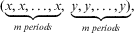 $$(\mathop{\underbrace{{x,x, \ldots, x}}}\limits_{\:m\;periods\:},\,\,\mathop{\underbrace{{y,y, \ldots, y)}}}\limits_{\:m\;periods\:},$$
with the horizontal axis representing x and the vertical axis representing y, for a type  $$${{\tau }_0}$$$
citizen and a type
 $$$\tau \ne {{\tau }_0}$$$
citizen. Note that the indifference curve of the type
 $$${{\tau }_0}$$$
citizen is flat at
 $$$({\rm{0}},{{x}_{{{\tau }_1}}})$$$
, reflecting the fact that
 $$${{u^{\prime}}_{{{\tau }_0}}}(0)\, = \,0$$$
, and the indifference curve of the type
 $$$\tau \ne {{\tau }_0}$$$
has a negative slope at
 $$$(0,{{x}_{{{\tau }_1}}})$$$
, reflecting the fact that
 $$${{u^{\prime}}_\tau }(0)\, \gt \,0$$$
.
Given the above description of punishments, any deviation by an office holder is followed by a lottery over strings
 $$(\mathop{\underbrace{{0,0, \ldots, 0}}}\limits_{\:m\;periods\:},\,\,\mathop{\underbrace{{{{x}_{{{\tau }_1}}},{{x}_{{{\tau }_1}}}, \ldots, {{x}_{{{\tau }_1}}}}}}\limits_{\:m\;periods\:})\:\;{\rm and}\;\:(\mathop{\underbrace{{0,0, \ldots, 0}}}\limits_{\:m\;periods\:},\,\,\mathop{\underbrace{{0,0, \ldots, 0,}}}\limits_{\:m\;periods\:})$$
with probability p 0 on the latter and 1 − p 0 on the former. These strings are indicated in Figure 1, and the indifference curves corresponding to the expected payoff from this punishment lottery are indicated by the heavy level sets in the figure for type  $$${{\tau }_0}$$$
and type
 $$$\tau \ne {{\tau }_0}$$$
politicians. To reconcile the incentives of office holders, choosing policy a must be weakly preferable to the punishment lottery for all types, and so the point (a, a) must belong to the lens formed by the indifference curves of the type
 $$${{\tau }_0}$$$
and all
 $$$\tau \ne {{\tau }_0}$$$
politicians. In Figure 2, we see that for the given setting of m, there is no policy a belonging to the lens of incentives that is also within ε of zero.
Lens of incentives
Note that the marginal rate of substitution between policy in the first m periods and in the next m periods is
 $$\frac{{(1\,{\rm{ - }}\,{{\delta }^m} ){{{u^{\prime}}}_\tau }(0)}}{{{{\delta }^m} (1\,{\rm{ - }}\,{{\delta }^m} ){{{u^{\prime}}}_\tau }({{x}_{{{\tau }_1}}})}}\, = \,\frac{{{{{u^{\prime}}}_\tau }(0)}}{{{{\delta }^m} {{{u^{\prime}}}_\tau }({{x}_{{{\tau }_1}}})}}.$$
Choosing m higher, so δ m becomes smaller, citizens put greater weight on the first m periods than the next m, making the indifference curves in Figure 1 steeper. The bulk of Step 1 consists of showing that when a is small, we can choose δ m in a critical range such that (a, a) is preferred to the punishment lottery by all citizen types; geometrically, the lens of incentives intersects the 45 degree line sufficiently close to the origin, as depicted in Figure 3. Once this is established, we can perform the construction for discount factors close to one: when δ is close to one, we can choose m so that δ m belongs to the critical range. This entails that the punishment lottery is worse than the constant policy a for 2 m periods for all types, and in addition we then specify that δ is close enough to one that the potential gain from any one-shot deviation is more than offset by the cost of entering the punishment phase.
Choosing a and δm
The punishment strategies used in Step 1 are in fact somewhat more complex than the simple description above, because (1) we must specify policies beyond the 2 m periods following a deviation, and because (2) we must address the possibility of deviations from the punishment strategies. Of particular importance, we must ensure that voters have incentives to re-elect the incumbent if, m+1 periods following a deviation, she chooses x = 0. This choice reveals that the politician is type  $$${{\tau }_0}$$$
, and voters then update that the office holder will continue to choose x = 0 in the next m − 1 periods if re-elected. The alternative is to elect a challenger and restart the punishment phase, but by construction of the punishment strategies, the challenger, if elected, will also choose x = 0 for m periods, regardless of her type. A disadvantage of electing a challenger to a type
 $$$\tau \ne {{\tau }_0}$$$
voter is that with probability p 0, the challenger is type
 $$${{\tau }_0}$$$
and will choose x = 0 for an additional m periods beyond the first m. The advantage of electing a challenger to such a voter is that with probability 1 − p 0, the politician will choose preferable policies after the first m terms of office. Figure 4 depicts the distribution over policy paths following a deviation. We specify that after the first 2 m periods following a deviation, a type
 $$$\tau \ne {{\tau }_0}$$$
office holder chooses
 $$$x = {{x}_{{{\tau }_1}}}$$$
, while a type
 $$${{\tau }_0}$$$
office holder alternately chooses
 $$$x = {{x}_{{{\tau }_1}}}$$$
for k periods and x = 0 for one period. When k is large, therefore, the benefit of electing a challenger to a type
 $$$\tau \ne {{\tau }_0}$$$
voter is outweighed by the cost, and a majority of voters indeed prefers to re-elect the incumbent.
Punishment paths
Step 3 provides a procedure for splicing equilibria that support the extreme policies from Steps 1 and 2. For example, consider two equilibria supporting xa and xb. To construct an equilibrium supporting the path (a,b,a,b,…), I specify, roughly, that the equilibrium construction from Step 1 be applied to histories consisting of odd periods, and that the construction from Step 2 be applied to histories consisting of even periods. Thus a deviation in an odd period t is punished in future odd periods; and moreover, in future even periods, we simulate punishments as though an analogous deviation had occurred in the previous even period t − 1. If an office holder chooses x ≠ a in Period 3, for example, then play in future even periods proceeds as though she had chosen x ≠ b in Period 2, so the incumbent is removed from office, and we commence with the punishments in Figure 4 in all future even and odd periods. This means that the newly elected office holder chooses x = 0 for the next m odd periods and x = 1 for the next m even periods. After that, play depends on the politician's type: if she is type  $$${{\tau }_0}$$$
, for example, then she chooses
 $$$x = {{x}_{{{\tau }_{n - 1}}}}$$$
in all subsequent even periods; and she chooses x = 0 in an additional m odd periods, then alternately chooses
 $$$x = {{x}_{{{\tau }_1}}}$$$
for k odd periods and x = 0 for one odd period. Because punishments in odd periods now alternate with even periods, payoffs in odd periods are now effectively discounted by δ 2 (and similarly for payoffs in even periods), so the construction requires a discount factor greater than the cutoffs from Steps 1 and 2; if xa is supported for discount factors above
 $$$\delta ^{\prime}$$$
and xb is supported for discount factors about
 $$$\delta ^{\prime\prime}$$$
, then the splicing procedure requires a discount factor above
 $$$\sqrt {\max \{ \delta ^{\prime},\delta ^{\prime\prime}\} } $$$
. Further details related to the transmission of information across odd and even periods arise as well. When an office holder chooses
 $$$x = {{x}_{{{\tau }_1}}}$$$
after m odd punishment periods, for example, she reveals that she is not type
 $$${{\tau }_0}$$$
, and the updated probability that she is type
 $$${{\tau }_n}$$$
increases; this means that she is more likely to choose x = 1 for an additional m even periods, and we must confirm that a majority of voters still has an incentive to re-elect the incumbent. These details are straightforward and are addressed in the proof.
With the splicing procedure defined, it can be used recursively to generate policy paths that alternate between a and b at nearly arbitrary frequencies. For example, we can splice equilibria supporting (a,a,a,a,…) and (a,b,a,b,…) to produce a perfect Bayesian electoral equilibrium that supports policy choice a with frequency 0.75.
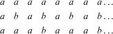 $$\matrix{ a &#x0026; a &#x0026; a &#x0026; a &#x0026; a &#x0026; a &#x0026; a &#x0026; {a \ldots } \cr a &#x0026; b &#x0026; a &#x0026; b &#x0026; a &#x0026; b &#x0026; a &#x0026; {b \ldots} \cr a &#x0026; a &#x0026; a &#x0026; b &#x0026; a &#x0026; a &#x0026; a &#x0026; {b \ldots } $$
And we can splice equilibria supporting a with frequency 0.5 and 0.75 to produce an equilibrium supporting a with frequency 0.625.
 $$\matrix{ a &#x0026; b &#x0026; a &#x0026; b &#x0026; a &#x0026; b &#x0026; a &#x0026; b &#x0026; a &#x0026; b &#x0026; a &#x0026; b &#x0026; a &#x0026; b &#x0026; a &#x0026; {b \ldots } \cr a &#x0026; a &#x0026; a &#x0026; b &#x0026; a &#x0026; a &#x0026; a &#x0026; b &#x0026; a &#x0026; a &#x0026; a &#x0026; b &#x0026; a &#x0026; a &#x0026; a &#x0026; {b \ldots } \cr a &#x0026; a &#x0026; a &#x0026; b &#x0026; a &#x0026; a &#x0026; b &#x0026; b &#x0026; a &#x0026; a &#x0026; a &#x0026; b &#x0026; a &#x0026; a &#x0026; b &#x0026; {b \ldots } $$
Thus, using this logic, we can apply the splicing procedure a finite number of times to approximate an arbitrary frequency to within any given level of precision; given  $$$\alpha \in [0,1]$$$
, for example, we can construct an equilibrium such that in sufficiently long runs of periods, the policy outcome is a with frequency
 $$$\hat{\alpha }$$$
close to α. Each application imposes a higher cutoff for the discount factor, but because only a finite number of iterations is required for a given level of precision, we can take the maximum required for each application of the procedure.
Step 4 uses the alternating equilibria from Step 3 to punish deviations from arbitrary paths of policies. Choose policies a, b ∈ X as in the theorem. Then use Steps 1 and 2 to choose  $$$a^{\prime} \in (0,\frac{a}{2})$$$
and
 $$$b^{\prime} \in \left( {\frac{{b\, + \,{\rm{1}}}}{2},1} \right)$$$
such that for discount factors sufficiently close to one, there exist perfect Bayesian electoral equilibria supporting
 $$${{{\bf {{x}}}}^{a^{\prime}}} $$$
and
 $$${{{\bf {{x}}}}^{b^{\prime}}} $$$
. Consider any path
 $$${\bf {{x}}} \in {{[a,b]}^\infty } $$$
in the interval [a,b]. Note that for a type
 $$$\tau $$$
citizen, the discounted utility from the path starting in period t+1, namely
 $$$({{x}_{t + 1}},{{x}_{t + 2}}, \ldots )$$$
, can be written as the integral
 $${{E}_{{{\lambda }_{t\, + \,1}}}}[{{u}_\tau }(x)]\, = \,\int {{u}_\tau }(x){{\lambda }_{t\, + \,1}}(dx)\, = \,(1\,{\rm{ - }}\,\delta )\mathop{\sum}\limits_{t^{\prime} = t\, + \,1}^\infty {{\delta }^{t^{\prime}\,{\rm{ - }}\,t\,{\rm{ - }}\,1}} {{u}_\tau }({{x}_{t^{\prime}}})$$
with respect to a probability measure λt +1 on [a,b], where I normalize payoffs by 1 − δ. In the space of utility imputations, depicted in Figure 5 for the case of n = 1, λt +1 induces a probability measure on the thick portion of the utility frontier, and the vector of expected utilities lies in the shaded region below the frontier. Moreover, each x in the support of λt +1 can be written as a strict convex combination of a′ and b′ with weight α(x) on a′ and 1 − α(x) on b′. By strict concavity, the convex combination
Extreme punishments
 $$\alpha (x){{u}_\tau }(a^{\prime})\, + \,(1\,{\rm{ - }}\,\alpha (x)){{u}_\tau }(b^{\prime})$$
is less than  $$${{u}_\tau }(x)$$$
by an increment
 $$$\eta \, \gt \,0$$$
that is uniform across
 $$$x \in [a,b]$$$
. Thus,
 $${ {{E}_{{{\lambda }_{t + 1}}}}[{{u}_\tau }(x)]\geq \int [\alpha (x){{u}_\tau }(a^{\prime}) + (1 - \alpha (x)){{u}_\tau }(b^{\prime}) + \eta ]d{{\lambda }_{t + 1}} \cr \!\!\!\!\!= {{E}_{{{\lambda }_{t + 1}}}}[\alpha (x)]{{u}_\tau }(a^{\prime}) + (1 - {{E}_{{{\lambda }_{t + 1}}}}[\alpha (x)]){{u}_\tau }(b^{\prime}) + \eta . \cr}$$
We can use the splicing procedure to approximate the weights  $$${{E}_{{{\lambda }_{t\, + \,1}}}}[\alpha (x)]$$$
and
 $$$1\,{\rm{ - }}\,{{E}_{{{\lambda }_{t\, + \,1}}}}[\alpha (x)]$$$
by
 $$$\hat{\alpha }$$$
and
 $$$1\,{\rm{ - }}\,\hat{\alpha }$$$
, so that the corresponding convex combination is uniformly
 $$$\frac{\eta }{2}$$$
less than
 $$${{E}_{{{\lambda }_{t\, + \,1}}}}[{{u}_\tau }(x)]$$$
, and we use the corresponding strategies from Step 3 to punish any deviation in period t.
For these punishments to deter all one-shot deviations, we must choose δ sufficiently close to one. Specifically, the punishment is effective if for all  $$$\tau $$$
,
 $$(1\,{\rm{ - }}\,\delta )\mathop {\max }\limits_x {{u}_\tau }(x)\, + \,\delta \Big({{E}_{{{\lambda }_{t\, + \,1}}}}[{{u}_\tau }(x)]\,{\rm{ - }}\,\frac{\eta }{2}\Big)\,\leq \,(1\,{\rm{ - }}\,\delta )\mathop {\min }\limits_y {{u}_\tau }(y)\, + \,\delta {{E}_{{{\lambda }_{t\, + \,1}}}}[{{u}_\tau }(x)],$$
and letting  $$${\rm{\rDelta }}\, = \,{\max }_{\tau, x,y} [{{u}_\tau }(x)\,{\rm{ - }}\,{{u}_\tau }(y)]$$$
denote the maximum gain from a one-shot deviation, the above inequality holds if
 $$${\rm{\rDelta }}\,\leq \,\frac{{\delta \eta }}{{2(1\,{\rm{ - }}\,\delta )}}$$$
, which holds for δ close to one. Thus, we can specify punishment strategies to deter any deviation in period t. Finally, the above discussion has fixed a period t+1 and the corresponding probability measure λt +1, but the set of probability measures with support in [a,b] is compact in the weak* topology, and the approximation
 $$$\hat{\alpha }$$$
and
 $$$1\,{\rm{ - }}\,\hat{\alpha }$$$
holds for an open set around λt +1, so the open covering generated by choice of
 $$$\hat{\alpha }$$$
as we vary λ must have a finite subcover. Thus, we can choose δ sufficiently close to one such that for all t, Step 3 can be applied to specify an effective punishment strategy to deter a deviation in period t, delivering the required perfect Bayesian electoral equilibrium.
Type-Dependent Paths
In this section, I give an informal argument for a corollary of the above theorem that extends the result to allow for policy paths to depend on the office holder's type. Let  $$$\xi :T \rightarrow {{[0,1]}^\infty } $$$
be a path assignment that associates to each type
 $$$\tau $$$
a path
 $$$\xi (\tau )\, = \,({{\xi }_1}(\tau ),{{\xi }_2}(\tau ), \ldots )$$$
of policies. Say the path assignment ξ is incentive compatible if the path associated with any type is no worse for that type than any other assigned path; that is, for all
 $$$\tau $$$
and
 $$$\tau ^{\prime}$$$
,
 $$\mathop{\sum}\limits_{t\, = \,1}^\infty {{\delta }^{t\,{\rm{ - }}\,1}} {{u}_\tau }({{\xi }_t}(\tau ))\,\geq \,\mathop{\sum}\limits_{t\, = \,1}^\infty {{\delta }^{t\,{\rm{ - }}\,1}} {{u}_\tau }({{\xi }_t}(\tau ^{\prime})).$$
Of course, if ξ is constant, so that the policy specified is independent of the office holder's type (the case considered in the theorem), then it is incentive compatible. A path assignment ξ is supportable given δ < 1 if there is a perfect Bayesian equilibrium such that along the path of play from the initial history, in every period t, the type  $$$\tau $$$
office holder chooses policy ξt(
 $$$\tau $$$
). Clearly, incentive compatibility is necessary for supportability; the following corollary establishes that when citizens are patient, it is essentially sufficient as well.
Corollary: For all  $$$a,b \in X$$$
with
 $$$0\, \lt \,a\, \lt \,b\, \lt \,1$$$
, there exists
 $$$\overline{\delta } \, \lt \,1$$$
such that for all
 $$$\delta \in (\overline{\delta }, 1)$$$
and all path assignments
 $$$\xi $$$
with
 $$$\xi (T) \subseteq {{[a,b]}^\infty } $$$
, if ξ is incentive compatible, then it is supportable given δ.
To establish the corollary, let ξ be an incentive-compatible path assignment such that for all  $$$\tau $$$
,
 $$$\xi (\tau ) \in {{[a,b]}^\infty }$$$
. To support this assignment, we specify that after a public history of length t − 1, such that a type
 $$$\tau $$$
politician has held office and chosen ‘correct’ policies
 $$$({{x}_1}, \ldots, {{x}_{t\,{\rm{ - }}\,1}})\, = \,({{\xi }_1}(\tau ), \ldots, {{\xi }_{t\,{\rm{ - }}\,1}}(\tau ))$$$
, the office holder chooses
 $$${{x}_t}\, = \,{{\xi }_t}(\tau )$$$
and is re-elected. Punishments are as follows. If past policy choices
 $$${{x}_1}, \ldots, {{x}_{t\,{\rm{ - }}\,1}}$$$
of an office holder are consistent with ξ, so that the set
 $$T({{x}_1}, \ldots, {{x}_{t\,{\rm{ - }}\,1}}|\xi )\, = \,\{ \tau \in T|({{\xi }_1}(\tau ), \ldots, {{\xi }_{t\,{\rm{ - }}\,1}}(\tau ))\, = \,({{x}_1}, \ldots, {{x}_{t\,{\rm{ - }}\,1}})\} $$
is nonempty, but xt is not consistent with these choices, then select any  $$$\tilde{\tau } \in T({{x}_1}, \ldots, {{x}_{t\,{\rm{ - }}\,1}}|\xi )$$$
, and use the punishments constructed in the proof of the theorem for a deviation from
 $$${{\xi }_t}(\tilde{\tau })$$$
. If xt is consistent with ξ but the office holder is not re-elected, then—given that voter beliefs may not place probability one on the office holder's true type (that is,
 $$$T({{x}_1}, \ldots, {{x}_{t\,{\rm{ - }}\,1}},{{x}_t}|\xi )$$$
may not be singleton)—we must specify punishments in a more nuanced way. Let
 $$$p({{x}_1}, \ldots, {{x}_t}|\xi )$$$
represent the voters’ posterior beliefs about the office holder's type, so that if the incumbent is re-elected, then a type
 $$$\tau $$$
voter's expected discounted utility is
 $$\mathop{\sum}\limits_{\tau ^{\prime}} {{p}_{\tau ^{\prime}}}({{x}_1}, \ldots, {{x}_t}|\xi )\mathop{\sum}\limits_{t^{\prime}\, = \,t\, + \,1}^\infty {{\delta }^{t^{\prime}\,{\rm{ - }}\,t\,{\rm{ - }}\,1}} {{u}_\tau }({{\xi }_{t^{\prime}}}(\tau ^{\prime})),$$
which is the expected utility with respect to a particular lottery  $$$\lambda ({{x}_1}, \ldots, {{x}_t}|\xi )$$$
. By the arguments of Step 4, we may specify that if the incumbent is not re-elected, then punishment strategies alternate between a′ and b′ at a frequency that yields a lower discounted utility for all voter types.
Choosing  $$$\overline{\delta } $$$
sufficiently close to one to offset the one-period gains from any deviation, the above punishment strategies support the path assignment ξ. In particular, consider the optimization problem of a type
 $$$\tau $$$
office holder in period t, assuming that she has chosen the correct policies
 $$$({{x}_1}, \ldots, {{x}_{t\,{\rm{ - }}\,1}})\, = \,({{\xi }_1}(\tau ), \ldots, {{\xi }_{t\,{\rm{ - }}\,1}}(\tau ))$$$
in all previous periods. The strategies above specify that she choose
 $$${{x}_t}\, = \,{{\xi }_t}(\tau )$$$
in period t and continue to follow the path
 $$${{\xi }_{t\, + \,1}}(\tau ),{{\xi }_{t\, + \,2}}(\tau ), \ldots $$$
thereafter. I claim that the politician cannot gain from deviating to the policies assigned to some other type
 $$$\tau ^{\prime} \in T({{x}_1}, \ldots, {{x}_{t\,{\rm{ - }}\,1}}|\xi )$$$
. Indeed, consider any
 $$$\tau ^{\prime} \in T({{x}_1}, \ldots, {{x}_{t\,{\rm{ - }}\,1}}|\xi )$$$
, and let
 $$$\xi (\tau )\, = \,({{x}_1},{{x}_2}, \ldots )$$$
and
 $$$\xi (\tau ^{\prime})\, = \,(x_{1}^{\prime}, x_{{\rm{2}}}^{\prime}, \ldots )$$$
denote the policies assigned to types
 $$$\tau $$$
and
 $$$\tau ^{\prime}$$$
. Note that
 $$\mathop{\sum}\limits_{t^{\prime}\, = \,t}^\infty {{\delta }^{t^{\prime}\,{\rm{ - }}\,t}} {{u}_\tau }({{x}_{t^{\prime}}})\geq \mathop{\sum}\limits_{t^{\prime}\, = \,t}^\infty {{\delta }^{t^{\prime}\,{\rm{ - }}\,t}} {{u}_\tau }({{x^\prime}_{t^{\prime}}})$$
holds, in light of the fact that  $$$(x_{1}^{\prime}, \ldots, x_{{t\,{\rm{ - }}\,1}}^{\prime} )\, = \,({{x}_1}, \ldots, {{x}_{t\,{\rm{ - }}\,1}})$$$
, if and only if
 $$\mathop{\sum}\limits_{t^{\prime}\, = \,1}^\infty {{\delta }^{t^{\prime}\,{\rm{ - }}\,t}} {{u}_\tau }({{x}_{t^{\prime}}})\,\geq \,\mathop{\sum}\limits_{t^{\prime}\, = \,1}^\infty {{\delta }^{t^{\prime}\,{\rm{ - }}\,t}} {{u}_\tau }({{x^\prime}_{t^{\prime}}}),$$
which holds by incentive compatibility, establishing the claim. Moreover, it cannot be profitable to follow the policies assigned to  $$$\tau ^{\prime} \in T({{x}_1}, \ldots, {{x}_{t\,{\rm{ - }}\,1}}|\xi )$$$
and deviate at a later point t′, as the punishment for deviating from
 $$${{\xi }_{t^{\prime}}}(\tau ^{\prime})$$$
is worse than following
 $$$\xi (\tau ^{\prime})$$$
for all types. Recall that if the office holder deviates to a policy
 $$${{x}_t}'$$$
that is inconsistent with ξ, then the strategies above invoke punishments for deviating from the policies of an arbitrary type
 $$$\tilde{\tau } \in T({{x}_1}, \ldots, {{x}_{t\,{\rm{ - }}\,1}}|\xi )$$$
. Since it is not profitable to follow the policies assigned to
 $$$\tilde{\tau }$$$
, and since the punishment for deviating from
 $$${{\xi }_t}(\tilde{\tau })$$$
is worse than following
 $$$\xi (\tilde{\tau })$$$
for all types, it cannot be profitable to deviate to policies that are inconsistent with ξ. We conclude that the office holder's expected discounted utility is maximized by following the path assignment.
Conclusion
This article shows that when citizens are sufficiently patient, arbitrary policy paths through arbitrarily large regions of the policy space can be generated as the result of equilibrium play. Thus in the absence of an a priori bound on discount factors, some form of stationarity that limits the extent of conditioning on histories is needed to generate empirically meaningful predictions. As mentioned in the introduction, the addition of moral hazard to the model would significantly alter the equilibrium analysis and limit the scope for punishment of politicians, so this modeling approach may yet entail substantial restrictions on equilibrium behavior. In lieu of this, or another departure from the pure adverse selection framework, the application of dynamic electoral models will rely on equilibrium refinements beyond the concept of perfect Bayesian electoral equilibrium considered in this article.
APPENDIX
Proof of Theorem
The proof proceeds in four steps.
Step 1: For all ε > 0, there exist  $$$a \in (0,{\epsilon})$$$
and
 $$$\hat{\delta } \in (0,1)$$$
such that for all
 $$$\delta \in (\hat{\delta },1)$$$
,
we have  $$${{{\bf {{x}}}}^a} \in P(\delta )$$$
.
Fix ε > 0. I begin by choosing parameters a,δ,β ∈ (0,1) with a < ε and a natural number k ≥ 1 to satisfy three inequalities (Inequalities 5–7 below) that are critical for the equilibrium construction. Following these choices, I will specify  $$$\hat{\delta }$$$
to satisfy three further inequalities, namely 12–14, and I determine a number m of periods used in punishment phases. First, choose k sufficiently large that for all
 $$$\tau \ne {{\tau }_0}$$$
, we have
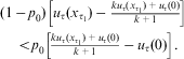 $$\matrix{(1\,{\rm{ - }}\,{{p}_0})\left[ {{{u}_\tau }({{x}_{{{\tau }_1}}})\,{\rm{ - }}\,\frac{{k{{u}_\tau }({{x}_{{{\tau }_1}}})\, + \,{{u}_\tau }(0)}}{{k\, + \,1}}} \right] \cr \; \; \lt {{p}_0}\left[ {\frac{{k{{u}_\tau }({{x}_{{{\tau }_1}}})\, + \,{{u}_\tau }(0)}}{{k\, + \,1}}\,{\rm{ - }}\,{{u}_\tau }(0)} \right]. \\ $$
For each  $$$\tau $$$
, define
 $${{W}_\tau }\, = \,\frac{1}{{1\,{\rm{ - }}\,{{\delta }^{k\, + \,1}} }}[(1\,{\rm{ - }}\,{{\delta }^k} ){{u}_\tau }({{x}_{{{\tau }_1}}})\, + \,{{\delta }^k} (1\,{\rm{ - }}\,\delta ){{u}_\tau }(0)],$$
which implicitly depends on k and δ. This is the discounted utility (normalized by 1 − δ) of alternating sequences of  $$$x\, = \,{{x}_{{{\tau }_1}}}$$$
for k periods and x = 0 for one period. Note that by l'Hôpital's rule, we have for all
 $$$\tau $$$
,
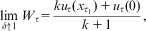 $$\mathop {\lim }\limits_{\delta \uparrow 1} {{W}_\tau } = \frac{{k{{u}_\tau }({{x}_{{{\tau }_1}}})\, + \,{{u}_\tau }(0)}}{{k\, + \,1}},$$
and in addition that
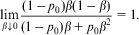 $$\mathop {\lim }\limits_{\beta \downarrow 0} \frac{{(1\,{\rm{ - }}\,{{p}_0})\beta (1\,{\rm{ - }}\,\beta )}}{{(1\,{\rm{ - }}\,{{p}_0})\beta \, + \,{{p}_0}{{\beta }^2} }}\, = \,1.$$
Using Inequalities 1–3, there exists  $$$\overline{\beta } \in (0,1)$$$
such that two conditions hold: (1) for all
 $$$\beta \in (0,\overline{\beta } )$$$
, we have
 $$2(1\,{\rm{ - }}\,{{p}_0})\beta (1\,{\rm{ - }}\,\beta )\, \gt \,(1\,{\rm{ - }}\,{{p}_0})\beta \, + \,{{p}_0}{{\beta }^2}, $$
and (2) there exists  $$$\underline{\delta } \, \in \,(0,1)$$$
such that for all
 $$$\delta \in (\underline{\delta }, 1)$$$
and all
 $$$\beta \in (0,\overline{\beta } )$$$
, we have for all
 $$$\tau \ne {{\tau }_0}$$$
,
 $$(1\,{\rm{ - }}\,{{p}_0})({{u}_\tau }({{x}_{{{\tau }_1}}})\,{\rm{ - }}\,{{W}_\tau })\, \lt \,{{p}_0}(1\,{\rm{ - }}\,\beta )({{W}_\tau }\,{\rm{ - }}\,{{u}_\tau }(0)).$$
Inequality 4 is used in the selection of a, below, and Inequality 5 is used to give voters proper incentives in the equilibrium construction.
Given  $$$\delta \in (\underline{\delta }, 1)$$$
and
 $$$\beta \in (0,\overline{\beta } )$$$
, the next inequality is used to address the incentives of type
 $$${{\tau }_0}$$$
office holders along the path of play:
 $$\matrix{(1\,{\rm{ - }}\,\delta )({{u}_{{{\tau }_0}}}(0)\,{\rm{ - }}\,{{u}_{{{\tau }_0}}}(a)) \hfill \cr \leq \delta [{{p}_0}[(1\,{\rm{ - }}\,{{\beta }^2} )({{u}_{{{\tau }_0}}}(a)\,{\rm{ - }}\,{{u}_{{{\tau }_0}}}(0))\, + \,{{\beta }^2} ({{u}_{{{\tau }_0}}}(a)\,{\rm{ - }}\,{{W}_{{{\tau }_0}}})] \hfill \cr + (1\,{\rm{ - }}\,{{p}_0})[(1\,{\rm{ - }}\,\beta )({{u}_{{{\tau }_0}}}(a)\,{\rm{ - }}\,{{u}_{{{\tau }_0}}}(0))\, + \,\beta ({{u}_{{{\tau }_0}}}(a)\,{\rm{ - }}\,{{u}_{{{\tau }_0}}}({{x}_{{{\tau }_1}}}))]]. \\ $$
The following inequality addresses incentives for type  $$$\tau \ne {{\tau }_0}$$$
office holders along the path of play: for all
 $$$\tau \ne {{\tau }_0}$$$
,
 $${ (1\,{\rm{ - }}\,\delta )\rDelta \leq &#x0026; \delta [{{p}_0}[(1\,{\rm{ - }}\,{{\beta }^2} )({{u}_\tau }(a)\,{\rm{ - }}\,{{u}_\tau }(0))\, + \,{{\beta }^2} ({{u}_\tau }(a)\,{\rm{ - }}\,{{W}_\tau })] \cr + &#x0026; (1\,{\rm{ - }}\,{{p}_0})[(1\,{\rm{ - }}\,\beta )({{u}_\tau }(a)\,{\rm{ - }}\,{{u}_\tau }(0))\, + \,\beta ({{u}_\tau }(a)\,{\rm{ - }}\,{{u}_\tau }({{x}_{{{\tau }_1}}}))], \cr}$$
where  $$$\rDelta \, = \,{\max }_{\tau, x,y} [{{u}_\tau }(x)\,{\rm{ - }}\,{{u}_\tau }(y)]$$$
. To see that Inequalities 6 and 7 are compatible for some
 $$$\delta \in (\underline{\delta }, 1)$$$
and some
 $$$\beta \in (0,\overline{\beta } )$$$
and for sufficiently small
 $$$a \in (0,{\epsilon})$$$
, define
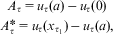 $$\matrix{{{A}_\tau }\, = \,{{u}_\tau }(a)\,{\rm{ - }}\,{{u}_\tau }(0) \cr A_{\tau }^{\ast} \, = \,{{u}_\tau }({{x}_{{{\tau }_1}}})\,{\rm{ - }}\,{{u}_\tau }(a), \\ $$
where these two quantities implicitly depend on a. It will be convenient to define  $$$\underline{A} \, = \,{\min }_{\tau \ne {{\tau }_0}} {{A}_\tau }$$$
and
 $$${{A}^\ast} \, = \,{\max }_{\tau \ne {{\tau }_0}} A_{\tau }^{\ast} $$$
. Of course,
 $$$\underline{A} \rightarrow 0$$$
and
 $$${{A}^\ast} \rightarrow {\max }_{\tau \ne {{\tau }_0}} [{{u}_\tau }({{x}_{{{\tau }_1}}})\,{\rm{ - }}\,{{u}_\tau }(0)]\, \gt \,0$$$
as a→0. Assuming without loss of generality that
 $$$a\, \lt \,{{x}_{{{\tau }_1}}}$$$
, the right-hand side of Inequality 6 is positive if
 $$\frac{{(1\,{\rm{ - }}\,{{p}_0})\beta }}{{1\, + \,{{p}_0}(\beta \,{\rm{ - }}\,{{\beta }^2} )\,{\rm{ - }}\,\beta }}\, \gt \,\frac{{{{u}_{{{\tau }_{\rm{0}}}}}(0)\,{\rm{ - }}\,{{u}_{{{\tau }_0}}}(a)}}{{{{u}_{{{\tau }_{\rm{0}}}}}(a)\,{\rm{ - }}\,{{u}_{{{\tau }_0}}}({{x}_{{{\tau }_1}}})}},$$
and using  $$${{u}_\tau }({{x}_{{{\tau }_1}}})\,\geq \,{{W}_\tau }$$$
, the right-hand side of Inequality 7 is positive if for all
 $$$\tau \ne {{\tau }_0}$$$
,
 $$\frac{{{{u}_\tau }(a)\,{\rm{ - }}\,{{u}_\tau }(0)}}{{{{u}_\tau }({{x}_{{{\tau }_1}}})\,{\rm{ - }}\,{{u}_\tau }(a)}}\, \gt \,\frac{{(1\,{\rm{ - }}\,{{p}_0})\beta \, + \,{{p}_0}{{\beta }^2} }}{{1\, + \,{{p}_0}(\beta \,{\rm{ - }}\,{{\beta }^2} )\,{\rm{ - }}\,\beta }}.$$
Note that
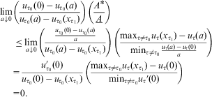 $${ \mathop {\lim }\limits_{a \downarrow 0} &#x0026; \left( {\frac{{{{u}_{{{\tau }_0}}}(0)\,{\rm{ - }}\,{{u}_{{{\tau }_0}}}(a)}}{{{{u}_{{{\tau }_0}}}(a)\,{\rm{ - }}\,{{u}_{{{\tau }_0}}}({{x}_{{{\tau }_1}}})}}} \right)\left( {\frac{{{{A}^\ast} }}{{\underline{A} }}} \right) \cr &#x0026; \leq \mathop {\lim }\limits_{a \downarrow 0} \left( {\frac{{\frac{{{{u}_{{{\tau }_0}}}(0)\,{\rm{ - }}\,{{u}_{{{\tau }_0}}}(a)}}{a}}}{{{{u}_{{{\tau }_0}}}(a)\,{\rm{ - }}\,{{u}_{{{\tau }_0}}}({{x}_{{{\tau }_1}}})}}} \right)\left( {\frac{{{{{\max }}_{\tau \ne {{\tau }_0}}}{{u}_\tau }({{x}_{{{\tau }_1}}})\,{\rm{ - }}\,{{u}_\tau }(a)}}{{{{{\min }}_{\tau \ne {{\tau }_0}}}\frac{{{{u}_\tau }(a)\,{\rm{ - }}\,{{u}_\tau }(0)}}{a}}}} \right) \cr &#x0026; = \frac{{u_{{{{\tau }_0}}}^{\prime} (0)}}{{{{u}_{{{\tau }_0}}}(0)\,{\rm{ - }}\,{{u}_{{{\tau }_0}}}({{x}_{{{\tau }_1}}})}}\left( {\frac{{{{{\max }}_{\tau \ne {{\tau }_0}}}{{u}_\tau }({{x}_{{{\tau }_1}}})\,{\rm{ - }}\,{{u}_\tau }(0)}}{{{{{\min }}_{\tau \ne {{\tau }_0}}}{{u}_\tau }'(0)}}} \right) \cr &#x0026; = 0. \cr}$$
Therefore, we can choose  $$$a \in (0,{\epsilon})$$$
and
 $$$\beta \in (0,\overline{\beta } )$$$
such that
 $$\frac{{(1\,{\rm{ - }}\,{{p}_0})\beta }}{{1\, + \,{{p}_0}(\beta \,{\rm{ - }}\,{{\beta }^2} )\,{\rm{ - }}\,\beta }}\, \gt \,\frac{{{{u}_{{{\tau }_0}}}(0)\,{\rm{ - }}\,{{u}_{{{\tau }_0}}}(a)}}{{{{u}_{{{\tau }_0}}}(a)\,{\rm{ - }}\,{{u}_{{{\tau }_0}}}({{x}_{{{\tau }_1}}})}}\, \gt \,\frac{1}{2} \cdot \frac{{(1\,{\rm{ - }}\,{{p}_0})\beta }}{{1\, + \,{{p}_0}(\beta \,{\rm{ - }}\,{{\beta }^2} )\,{\rm{ - }}\,\beta }},$$
automatically fulfilling Inequality 8, and such that for all  $$$\tau \ne {{\tau }_0}$$$
,
 $$\frac{{{{u}_{{{\tau }_0}}}(0)\,{\rm{ - }}\,{{u}_{{{\tau }_0}}}(a)}}{{{{u}_{{{\tau }_0}}}(a)\,{\rm{ - }}\,{{u}_{{{\tau }_0}}}({{x}_{{{\tau }_1}}})}}\, \lt \,\frac{1}{4} \cdot \frac{{{{u}_\tau }(a)\,{\rm{ - }}\,{{u}_\tau }(0)}}{{{{u}_\tau }({{x}_{{{\tau }_1}}})\,{\rm{ - }}\,{{u}_\tau }(a)}}.$$
Combining Inequalities 10 and 11 and using Inequality 4, we have
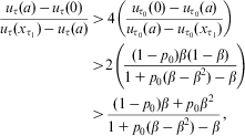 $${ \frac{{{{u}_\tau }(a)\,{\rm{ - }}\,{{u}_\tau }(0)}}{{{{u}_\tau }({{x}_{{{\tau }_1}}})\,{\rm{ - }}\,{{u}_\tau }(a)}}\, \gt \, 4\left( {\frac{{{{u}_{{{\tau }_0}}}(0)\,{\rm{ - }}\,{{u}_{{{\tau }_0}}}(a)}}{{{{u}_{{{\tau }_0}}}(a)\,{\rm{ - }}\,{{u}_{{{\tau }_0}}}({{x}_{{{\tau }_1}}})}}} \right) \cr \gt 2\left( {\frac{{(1\,{\rm{ - }}\,{{p}_0})\beta (1\,{\rm{ - }}\,\beta )}}{{1\, + \,{{p}_0}(\beta \,{\rm{ - }}\,{{\beta }^2} )\,{\rm{ - }}\,\beta }}} \right) \cr \gt \frac{{(1\,{\rm{ - }}\,{{p}_0})\beta \, + \,{{p}_0}{{\beta }^2} }}{{1\, + \,{{p}_0}(\beta \,{\rm{ - }}\,{{\beta }^2} )\,{\rm{ - }}\,\beta }}, \cr}$$
fulfilling Inequality 9, as required. It follows that for these choices of a and β, the right-hand sides of Inequality 6 and 7 are positive, and we can therefore choose  $$$\delta \in (\underline{\delta }, 1)$$$
sufficiently close to one to satisfy Inequalities 6 and 7.
Fixing a as above, note that there is some latitude in the choice of β, as Inequalities 8 and 9 involve strict inequalities. Next, I exploit this flexibility to choose  $$$\hat{\delta }$$$
close to one and fulfill the statement of Step 1. To do so, let
 $$${{\beta }_1},{{\beta }_2} \in (0,\overline{\beta } )$$$
be such that β 1 < β 2 and for all
 $$$\beta \in [{{\beta }_1},{{\beta }_2}]$$$
, Inequalities 8 and 9 hold. Then choose
 $$$\hat{\delta } \in (\underline{\delta }, 1)$$$
sufficiently high that for all
 $$$\delta \in (\hat{\delta },1)$$$
and all
 $$$\beta \in [{{\beta }_1},{{\beta }_2}]$$$
, Inequalities 6 and 7 hold in addition to Inequality 5, so that we have for all
 $$$\tau \ne {{\tau }_0}$$$
,
 $$(1\,{\rm{ - }}\,\delta )\rDelta \, \lt \,\delta {{p}_0}[\beta (1\,{\rm{ - }}\,\beta )({{u}_\tau }({{x}_{{{\tau }_1}}})\,{\rm{ - }}\,{{u}_\tau }(0))\, + \,{{\beta }^2} ({{u}_\tau }({{x}_{{{\tau }_1}}})\,{\rm{ - }}\,{{W}_\tau })]$$
 $$\!\!\!\!\!\!\!\!\!\!\!\!\!\!\!\!\!\!\!\!\!\!\!\!\!\!\!\!\!\!\!\!\!\!\!\!\!\!\!\!\!\!\!\!\!\!\!\!\!\!\!\!\!\!\!\!\!\!\!\!\!\!\!\!\!\!\!\!\!\!\!\!\!\!\!(1\,{\rm{ - }}\,\delta ){\rm{\rDelta }}\, \lt \,\delta {{p}_0}({{u}_\tau }({{x}_{{{\tau }_1}}})\,{\rm{ - }}\,{{W}_\tau })$$
 $$\!\!\!\!\!\!\!\!\!\!\!\!\!\!\!\!\!\!\!\!\!\!\!\!\!\!\!\!\!\!\!\!\!\!\!\!\!\!\!\!\!\!\!\!\!\!\!\!\!\!\!\!\!\!\!\!(1\,{\rm{ - }}\,\delta )\rDelta \, \lt \,\delta (1\,{\rm{ - }}\,{{p}_0})({{W}_{{{\tau }_0}}}\,{\rm{ - }}\,{{u}_{{{\tau }_0}}}({{x}_{{{\tau }_1}}})),$$
and so that  $$$\hat{\delta }{{\beta }_2}\, \gt \,{{\beta }_1}$$$
. Inequalities 12 and 13 are used to address incentives of type
 $$$\tau \ne {{\tau }_0}$$$
office holders, and Inequality 14 is used to address type
 $$${{\tau }_0}$$$
office holders, in the punishment phases.
Next, I determine a number m of periods to be used in punishment phases, as a function of  $$$\delta \in (\hat{\delta },1)$$$
. Using the inequality
 $$$\hat{\delta }{{\beta }_2} \gt {{\beta }_1}$$$
, I claim that for each
 $$$\delta \, \gt \,\hat{\delta }$$$
, there exists m such that
 $$${{\delta }^m} \in ({{\beta }_1},{{\beta }_2})$$$
. Indeed, we have
 $$$\delta \, \gt \,{{\beta }_1}$$$
by assumption, and
 $$${{\delta }^m} \, \lt \,\beta $$$
for sufficiently high m. The claim holds with m = 1 if
 $$$\delta \, \lt \,{{\beta }_2}$$$
. Otherwise,
 $$$\delta \,\geq \,{{\beta }_2}$$$
, and we can let m − 1 be the smallest natural number such that
 $$${{\delta }^{m\,{\rm{ - }}\,1}} \,\geq \,{{\beta }_2}$$$
. Then we have
 $$${{\delta }^m} \, \lt \,{{\beta }_2}$$$
and
 $$${{\delta }^m} \, = \,\delta {{\delta }^{m\,{\rm{ - }}\,1}} \,\geq \,\delta {{\beta }_2}\, \gt \,{{\beta }_1}$$$
, so that
 $$${{\delta }^m} \in ({{\beta }_1},{{\beta }_2})$$$
, as claimed. The remainder of the construction takes such m as given.
Now, given discount factor  $$$\delta \, \gt \,\hat{\delta }$$$
and m as above, I specify strategies and beliefs that support the constant path
 $$${{{\bf {{x}}}}^a} \, = \,(a,a, \ldots )$$$
. Note that by the preceding argument, we can choose m so that Inequalities 6 and 7 are satisfied by specifying
 $$$\beta \, = \,{{\delta }^m} \, \in \,({{\beta }_1},{{\beta }_2})$$$
. In the construction, I assume that voter beliefs about an untried challenger are given by the prior p, and that beliefs along an office holder's personal path of play are derived from Bayesian updating, and that off the politician's personal path of play, voters believe that with probability one the incumbent is type
 $$${{\tau }_0}$$$
. Strategies and beliefs are specified by assigning each history to one of five phases below, three of which are parameterized by a natural number j, and one of those is partitioned into three sub-phases, depending on voter beliefs. Phases 2–4 are used to punish deviations along the path of play, which takes place in Phase 1, and Phase 5 is used to punish deviations in the punishment phases.
Phase 1. All types of office holder choose x = a. If the incumbent chooses x = a, then all voters’ beliefs are given by the prior p, and all voters vote for the incumbent; and if the incumbent chooses  $$$x \ne a$$$
, then all voters believe that with probability one the incumbent is type
 $$${{\tau }_0}$$$
, and all type
 $$$\tau \,\geq \,{{\tau }_1}$$$
voters vote for the challenger, and type
 $$${{\tau }_0}$$$
voters vote for the incumbent.
Phase 2(j). All types of office holder choose x = 0. If the incumbent chooses x = 0, then all voters’ beliefs are given by the prior p, and all type  $$$\tau \,\geq \,{{\tau }_1}$$$
voters vote for the incumbent and type
 $$${{\tau }_0}$$$
voters vote for the challenger; and if the incumbent chooses
 $$$x\, \ne \,0$$$
, then all voters believe that with probability one the incumbent is type
 $$${{\tau }_0}$$$
, and all type
 $$$\tau \,\geq \,{{\tau }_1}$$$
voters vote for the challenger, and type
 $$${{\tau }_0}$$$
voters vote for the incumbent.
Phase 3(j). The type  $$${{\tau }_0}$$$
office holder chooses x = 0, and all type
 $$$\tau \ne {{\tau }_0}$$$
office holders choose
 $$$x\, = \,{{x}_{{{\tau }_1}}}$$$
. If the incumbent chooses x = 0, then all voters believe that with probability one the incumbent is type
 $$${{\tau }_0}$$$
, and all type
 $$$\tau \,\geq \,{{\tau }_1}$$$
voters vote for the incumbent, and type
 $$${{\tau }_0}$$$
voters vote for the challenger; if
 $$$x\, = \,{{x}_{{{\tau }_1}}}$$$
, then all voters’ beliefs are given by
 $$$\hat{p}$$$
, the updated prior conditional on the politician's type being not equal to
 $$${{\tau }_0}$$$
; and all type
 $$$\tau \,\geq \,{{\tau }_1}$$$
voters vote for the incumbent, and type
 $$${{\tau }_0}$$$
voters vote for the challenger; and otherwise, if
 $$$x \, \notin \, \{ 0,{{x}_{{{\tau }_1}}}\} $$$
, then all voters believe that with probability one the incumbent is type
 $$${{\tau }_0}$$$
, and all type
 $$$\tau \,\geq \,{{\tau }_1}$$$
voters vote for the challenger, and type
 $$${{\tau }_0}$$$
voters vote for the incumbent.
Phase 4.0(j). Type  $$${{\tau }_0}$$$
office holders choose
 $$$x\, = \,{{x}_{{{\tau }_1}}}$$$
if
 $$$j \in \{ 1, \ldots, k\} $$$
, they choose x = 0 if j = k+1, and type
 $$$\tau \ne {{\tau }_0}$$$
office holders choose
 $$$x = {{x}_{{{\tau }_1}}}$$$
for all
 $$$j\, = \,1, \ldots, k\, + \,1$$$
. All voters believe that with probability one the incumbent is type
 $$${{\tau }_0}$$$
. If
 $$$j \in \{ 1, \ldots, k\} $$$
and the incumbent chooses
 $$$x = {{x}_{{{\tau }_1}}}$$$
, or if j = k+1 and
 $$$x \in \{ 0,{{x}_{{{\tau }_1}}}\} $$$
, then all type
 $$$\tau \,\geq \,{{\tau }_1}$$$
voters vote for the incumbent, and type
 $$${{\tau }_0}$$$
voters vote for the challenger; and otherwise, type
 $$$\tau \,\geq \,{{\tau }_1}$$$
voters vote for the challenger, and type
 $$${{\tau }_0}$$$
voters vote for the incumbent.
Phase 4.1. Type  $$$\tau \ne {{\tau }_0}$$$
office holders choose
 $$$x\, = \,{{x}_{{{\tau }_1}}}$$$
and type
 $$${{\tau }_0}$$$
office holders choose x = 0. If the incumbent chooses
 $$$x\, = \,{{x}_{{{\tau }_1}}}$$$
, then all voters’ beliefs are given by
 $$$\hat{p}$$$
, the updated prior conditional on the politician's type being not equal to
 $$${{\tau }_0}$$$
, and all type
 $$$\tau \,\geq \,{{\tau }_1}$$$
voters vote for the incumbent, and type
 $$${{\tau }_0}$$$
voters vote for the challenger; and otherwise, if
 $$$x \ne {{x}_{{{\tau }_1}}}$$$
, then all voters believe that with probability one the incumbent is type
 $$${{\tau }_0}$$$
, and all type
 $$$\tau \,\geq \,{{\tau }_1}$$$
voters vote for the challenger, and type
 $$${{\tau }_0}$$$
voters vote for the incumbent.
Phase 4.2. Type  $$$\tau \ne {{\tau }_0}$$$
office holders choose
 $$$x\, = \,{{x}_{{{\tau }_1}}}$$$
and type
 $$${{\tau }_0}$$$
office holders choose x = 0. If the incumbent chooses
 $$$x\, = \,{{x}_{{{\tau }_1}}}$$$
, then all voters’ beliefs are given by
 $$$\hat{p}$$$
, the updated prior conditional on the politician's type being not equal to
 $$${{\tau }_0}$$$
, and all type
 $$$\tau \,\geq \,{{\tau }_1}$$$
voters vote for the incumbent and type
 $$${{\tau }_0}$$$
voters vote for the challenger; and if the incumbent chooses x = 0, then all voters believe that with probability one the politician is type
 $$${{\tau }_0}$$$
, and all type
 $$$\tau \,\geq \,{{\tau }_1}$$$
voters vote for the incumbent and type
 $$${{\tau }_0}$$$
voters vote for the challenger; and if the incumbent chooses
 $$$x \, \notin \, \{ 0,{{x}_{{{\tau }_1}}}\} $$$
, then voters believe that with probability one the politician is type
 $$${{\tau }_0}$$$
, all type
 $$$\tau \,\geq \,{{\tau }_1}$$$
voters vote for the challenger, and type
 $$${{\tau }_0}$$$
voters vote for the incumbent.
Phase 5. All types of office holder choose their ideal policies. All voters believe that with probability one the incumbent is type  $$${{\tau }_0}$$$
, and all type
 $$$\tau \,\geq \,{{\tau }_1}$$$
voters vote for the challenger, and all type
 $$${{\tau }_0}$$$
voters vote for the incumbent.
The specification is completed by assigning the initial history Ø to Phase 1, and by defining the rule for transitioning between the phases.
• In Phase 1, if the office holder chooses x = a, then remain in Phase 1; if the office holder chooses x ≠ a and is re-elected, then move to Phase 5; and if the office holder chooses x ≠ a and is not re-elected, then move to Phase 2(1).
• In Phase 2(j), if the office holder chooses x = 0 and is re-elected, or if x ≠ 0 and the incumbent is not re-elected, then move to Phase 2 (j+1) if j < m and to Phase 3(1) if j = m; if the office holder chooses x = 0 and is not re-elected, then move to Phase 2(1); and if the office holder chooses x ≠ 0 and is re-elected, then move to Phase 5.
• In Phase 3(j), if the office holder chooses x = 0 and is re-elected, then move to Phase 3(j+1) if j < m and to Phase 4.0(1) if j = m; if the office holder chooses
 $$$x\, = \,{{x}_{{{\tau }_1}}}$$$
and is re-elected, then move to Phase 3(j+1) if j < m and to Phase 4.1 if j = m; if the office holder chooses
$$$x \, \notin \, \{ 0,{{x}_{{{\tau }_1}}}\} $$$
and is re-elected, then move to Phase 5; if the office holder chooses
$$$x \in \{ 0,{{x}_{{{\tau }_1}}}\} $$$
and is not re-elected, then move to Phase 2(1); and if the office holder chooses
$$$x \, \notin \, \{ 0,{{x}_{{{\tau }_1}}}\} $$$
and is not re-elected, then move to Phase 4.2.
• In Phase 4.0(j), first suppose the incumbent is re-elected. If
$$$j \in \{ 1, \ldots, k\} $$$
and the incumbent chooses
$$$x\, = \,{{x}_{{{\tau }_1}}}$$$
, then move to Phase
$$$4.0(j\, + \,1)$$$
; if
$$$j \in \{ 1, \ldots, k\} $$$
and the incumbent chooses
$$$x \ne {{x}_{{{\tau }_1}}}$$$
, then move to Phase 5; if j = k+1 and
$$$x \in \{ 0,{{x}_{{{\tau }_1}}}\} $$$
, then move to Phase 4.0(1); and if j = k+1 and
$$$x \, \notin \, \{ 0,{{x}_{{{\tau }_1}}}\} $$$
, then move to Phase 5. Supposing the incumbent is not re-elected, if
$$$j \in \{ 1, \ldots, k\} $$$
and the incumbent chooses
$$$x\, = \,{{x}_{{{\tau }_1}}}$$$
, or if j = k+1 and
$$$x\, = \,\{ 0,{{x}_{{{\tau }_1}}}\} $$$
, then move to Phase 2(1); and otherwise, move to Phase 4.2.• In Phase 4.1, if the office holder chooses
$$$x\, = \,{{x}_{{{\tau }_1}}}$$$
and is re-elected, then remain in Phase 4.1; if the office holder chooses
$$$x\, \ne \,{{x}_{{{\tau }_1}}}$$$
and is re-elected, then move to Phase 5; if the office holder chooses
$$$x\, = \,{{x}_{{{\tau }_1}}}$$$
and is not re-elected, then move to Phase 2(1); and if the office holder chooses
$$$x\, \ne \,{{x}_{{{\tau }_1}}}$$$
and is not re-elected, then move to Phase 4.2.• In Phase 4.2, if the office holder chooses x = 0 and is re-elected, then move to Phase 4.0(1); if the office holder chooses
$$$x\, = \,{{x}_{{{\tau }_1}}}$$$
and is re-elected, then move to Phase 4.1; if the office holder chooses
$$$x \, \notin \, \{ 0,{{x}_{{{\tau }_1}}}\} $$$
and is re-elected, then move to Phase 5; if the office holder chooses
$$$x \in \{ 0,{{x}_{{{\tau }_1}}}\} $$$
and is not re-elected, then move to Phase 2(1); and if the office holder chooses
$$$x \, \notin \, \{ 0,{{x}_{{{\tau }_1}}}\} $$$
and is not re-elected, then remain in Phase 4.2.• In Phase 5, if the office holder is re-elected, then remain in Phase 5; and otherwise, if the incumbent is not re-elected, then move to Phase 2(1).


This assignment of histories to phases entails a specification of strategies and beliefs. In order to verify that they form a perfect Bayesian equilibrium, I will focus on the most critical best-response conditions, addressing the more straightforward conditions with less formal arguments. I do not consider the votes of type  $$${{\tau }_0}$$$
voters, as they do not affect electoral outcomes.
It is useful to describe the paths of play at the beginning of Phases 1–5. Of course, the path of play beginning in Phase 1 is simply policy choice a and re-election, ad infinitum. Beginning in Phase 2(1), policy x = 0 is chosen for m periods and the incumbent is re-elected. Beginning in Phase 3(1), if the office holder is type  $$${{\tau }_0}$$$
, then she chooses x = 0 and is re-elected for m periods; and otherwise, if the office holder is type
 $$$\tau \ne {{\tau }_0}$$$
, then she chooses
 $$${{x}_{{{\tau }_1}}}$$$
and is re-elected for m periods. We then move to Phase 4.0 or 4.1, depending on whether the office holder is type
 $$${{\tau }_0}$$$
or
 $$$\tau \ne {{\tau }_0}$$$
. In the latter case, the office holder chooses
 $$$x\, = \,{{x}_{{{\tau }_1}}}$$$
and is re-elected ad infinitum; and in the former case, the office holder alternately chooses
 $$$x\, = \,{{x}_{{{\tau }_1}}}$$$
for k periods and x = 0 for one period, and is re-elected ad infinitum. In Phase 5, all types of office holder choose their ideal policies. When this phase is reached, voters believe the office holder is type
 $$${{\tau }_0}$$$
, the politician is removed from office, and we move to Phase 2 with the challenger assuming office.
Next, I calculate the continuation value (normalized by 1 − δ) of each citizen type at the beginning of Phase 2(1) after electing an untried challenger:
 $${{V}_\tau }\, = \,{{p}_0}[(1\,{\rm{ - }}\,{{\delta }^{2m}} ){{u}_\tau }(0)\, + \,{{\delta }^{2m}} {{W}_\tau }]\, + \,(1\,{\rm{ - }}\,{{p}_0})[(1\,{\rm{ - }}\,{{\delta }^m} ){{u}_\tau }(0)\, + \,{{\delta }^m} {{u}_\tau }({{x}_{{{\tau }_1}}})].$$
This reflects the fact that with probability p 0 the office holder is type  $$${{\tau }_0}$$$
and chooses x = 0 for 2 m periods and then alternately chooses
 $$$x\, = \,{{x}_{{{\tau }_1}}}$$$
for k periods and x = 0 for one period; and with probability 1 − p 0 the office holder is type
 $$$\tau \ne {{\tau }_0}$$$
and chooses x = 0 for m periods and chooses
 $$$x\, = \,{{x}_{{{\tau }_1}}}$$$
thereafter. I employ the one-shot deviation principle to confirm that no office holders of any type can gain by deviating, and that all voter types (in particular, types
 $$$\tau \geq {{\tau }_1}$$$
in Phases 2 and 3) vote as though pivotal.
Phase 1: First, consider the choice of a type  $$${{\tau }_0}$$$
office holder. Following the above strategy, the politician chooses x = a and is continually re-elected. Following any deviation, the politician is removed from office, so the best one-shot deviation is to choose x = 0 and to receive
 $$${{V}_{{{\tau }_0}}}$$$
in expectation after that. The one-shot deviation is unprofitable if
 $${{u}_{{{\tau }_0}}}(a)\,\geq \,(1\,{\rm{ - }}\,\delta ){{u}_{{{\tau }_0}}}(0)\, + \,\delta {{V}_{{{\tau }_0}}},$$
or equivalently,
 $$\hskip-12.5pc(1\,{\rm{ - }}\,\delta )({{u}_{{{\tau }_0}}}(0)\,{\rm{ - }}\,{{u}_{{{\tau }_0}}}(a))$$
 $$\!\!\!\!\!\!\!\!\!\!\!\!\!\!\!\!\leq \delta [{{p}_0}[(1\,{\rm{ - }}\,{{\delta }^{2m}} )({{u}_{{{\tau }_0}}}(a)\,{\rm{ - }}\,{{u}_{{{\tau }_0}}}(0))\, + \,{{\delta }^{2m}} ({{u}_{{{\tau }_0}}}(a)\,{\rm{ - }}\,{{W}_{{{\tau }_0}}})]$$
 $$ + (1\,{\rm{ - }}\,{{p}_0})[(1\,{\rm{ - }}\,{{\delta }^m} )({{u}_{{{\tau }_0}}}(a)\,{\rm{ - }}\,{{u}_{{{\tau }_0}}}(0))\, + \,{{\delta }^m} ({{u}_{{{\tau }_0}}}(a)\,{\rm{ - }}\,{{u}_{{{\tau }_0}}}({{x}_{{{\tau }_1}}}))]],$$
which after substituting  $$$\beta = {{\delta }^m} $$$
is equivalent to Inequality 6. Next, consider a type
 $$$\tau \ne {{\tau }_0}$$$
office holder. The best one-shot deviation is to choose
 $$$x = {{x}_\tau }$$$
followed by
 $$${{V}_\tau }$$$
. The one-shot deviation is unprofitable if
 $${{u}_\tau }(a)\,\geq \,(1\,{\rm{ - }}\,\delta ){{u}_\tau }({{x}_\tau })\, + \,\delta {{V}_\tau },$$
which is implied by
 $$(1\,{\rm{ - }}\,\delta )\rDelta \,\leq \,\delta [{{p}_0}[(1\,{\rm{ - }}\,{{\delta }^{2m}} )({{u}_\tau }(a)\,{\rm{ - }}\,{{u}_\tau }(0))\, + \,{{\delta }^{2m}} ({{u}_\tau }(a)\,{\rm{ - }}\,{{W}_\tau })]$$
 $$ + (1\,{\rm{ - }}\,{{p}_0})[(1\,{\rm{ - }}\,{{\delta }^m} )({{u}_\tau }(a)\,{\rm{ - }}\,{{u}_\tau }(0))\, + \,{{\delta }^m} ({{u}_\tau }(a)\,{\rm{ - }}\,{{u}_\tau }({{x}_{{{\tau }_1}}}))]]$$
which after substituting β = δ m is equivalent to Inequality 7.
Now consider a voter of any type. In case the incumbent chooses x = a, if the incumbent is re-elected, then she will continue to choose a and be re-elected. If a challenger is elected, then we remain in Phase 1, and the newly elected office holder continues to choose a. Thus, all voters are indifferent between the incumbent and a challenger, and voting for the incumbent is consistent with being pivotal. In case the incumbent chooses x ≠ a, then all voters believe that with probability one the politician is type  $$${{\tau }_0}$$$
. If the incumbent is re-elected, then we move to Phase 5, and voters expect that the office holder will choose
 $$$x\, = \,{{x}_{{{\tau }_0}}}\, = \,0$$$
, and then an untried challenger is elected, and we move to Phase 2(1). If the challenger is elected, then we move directly to Phase 2(1). Thus, the expected discounted payoff from electing a challenger exceeds that from re-electing the incumbent for a type
 $$$\tau \,\geq \,{{\tau }_1}$$$
voter if
 $${{V}_\tau }\,\geq \,(1\,{\rm{ - }}\,\delta ){{u}_\tau }(0)\, + \,\delta {{V}_\tau },$$
which indeed holds.
Phase 2 (j). First, consider the choice of a type  $$${{\tau }_0}$$$
office holder. Following the above strategy, the politician chooses x = 0 and is re-elected for m − j periods, after which we move to Phase 3(1) and she chooses x = 0 for m more periods, after which we move to Phase 4.0(1) and she alternately chooses
 $$$x\, = \,{{x}_{{{\tau }_1}}}$$$
for k periods and x = 0 for one period. Following any deviation, the politician is removed from office, we continue to Phase 2 (j+1) if j < m or to Phase 3(1) if j = m, and clearly the office holder receives a higher payoff by choosing her ideal policy and avoiding the election of a type
 $$$\tau \ne {{\tau }_0}$$$
challenger. Next, consider the choice of a type
 $$$\tau \ne {{\tau }_0}$$$
office holder. Following the above strategy, the politician chooses
 $$$x\, = \,0$$$
and is re-elected for m − j periods, and then chooses
 $$$x\, = \,{{x}_{{{\tau }_1}}}$$$
and is continually re-elected. The best one-shot deviation is to choose
 $$$x\, = \,{{x}_\tau }$$$
, after which the politician is removed from office, and we move to Phase 2 (j+1) or 3(1) with a new office holder. The incentives to deviate are maximal when j = 1, as then the cost of deviating is realized with probability p 0 after m − 1 periods. The one-shot deviation is unprofitable if
 $$(1\,{\rm{ - }}\,\delta ){{u}_\tau }(0)\, + \,\delta [(1\,{\rm{ - }}\,{{\delta }^{m\,{\rm{ - }}\,1}} ){{u}_\tau }(0)\, + \,{{\delta }^{m\,{\rm{ - }}\,1}} {{u}_\tau }({{x}_{{{\tau }_1}}})]$$
 $$\quad\ \ \ \ \geq (1\,{\rm{ - }}\,\delta ){{u}_\tau }({{x}_\tau })\, + \,\delta [{{p}_0}[(1\,{\rm{ - }}\,{{\delta }^{2m\,{\rm{ - }}\,1}} ){{u}_\tau }(0)\, + \,{{\delta }^{2m\,{\rm{ - }}\,1}} {{W}_\tau }]$$
 $$ \!\!\!\!\!\!\!\!\!\!\!\!+ (1\,{\rm{ - }}\,{{p}_0})[(1\,{\rm{ - }}\,{{\delta }^{m\,{\rm{ - }}\,1}} ){{u}_\tau }(0)\, + \,{{\delta }^{m\,{\rm{ - }}\,1}} {{u}_\tau }({{x}_{{{\tau }_1}}})]],$$
which is implied by
 $$(1\,{\rm{ - }}\,\delta )\rDelta \,\leq \,\delta {{p}_0}[{{\delta }^{m\,{\rm{ - }}\,1}} (1\,{\rm{ - }}\,{{\delta }^m} )({{u}_\tau }({{x}_{{{\tau }_1}}})\,{\rm{ - }}\,{{u}_\tau }(0))\, + \,{{\delta }^{2m\,{\rm{ - }}\,1}} ({{u}_\tau }({{x}_{{{\tau }_1}}})\,{\rm{ - }}\,{{W}_\tau })],$$
which after substituting  $$$\beta \, = \,{{\delta }^m} $$$
is implied by Inequality 12.
Now consider a type  $$$\tau \,\geq \,{{\tau }_1}$$$
voter. In case the incumbent chooses x = 0, then the voters’ beliefs about the incumbent's type are given by the prior p. If the incumbent is re-elected, then she will choose x = 0 for m − 1 more periods, and we move to Phase 3(1). If the challenger is elected, then we move back to Phase 2(1). Thus the expected discounted payoff to the type
 $$$\tau \,\geq \,{{\tau }_1}$$$
voter from re-electing the incumbent is greater than from electing a challenger. In case the incumbent chooses
 $$$x\, \ne \,0$$$
, then the voters believe that with probability one the politician is type
 $$${{\tau }_0}$$$
. If the incumbent is re-elected, then we move to Phase 5, and she chooses x = 0, is removed from office, and we move to Phase 2(1). If the challenger is elected, then we remain in Phase 2 for m − 1 more periods, and we move to Phase 3(1). Thus the expected discounted payoff of electing the challenger is greater for the type
 $$$\tau \ne {{\tau }_0}$$$
voter than that of re-electing the incumbent.
Phase 3(j). First, consider the choice of a type  $$${{\tau }_0}$$$
office holder. Following the above strategy, the politician chooses x = 0 and is re-elected for m − j more periods, after which we move to Phase 4.0(1) and she alternately chooses
 $$$x\, = \,{{x}_{{{\tau }_1}}}$$$
for k periods and x = 0 for one period. Following any deviation
 $$$x^{\prime} \, \notin \, \{ 0,{{x}_{{{\tau }_1}}}\} $$$
, the politician is removed from office, and we move to Phase 4.2, where a challenger is elected and chooses policy. If the newly elected office holder is type
 $$${{\tau }_0}$$$
, then she chooses x = 0, and we move to Phase 4.0(1); and if she is type
 $$$\tau \ne {{\tau }_0}$$$
, then she chooses
 $$$x\, = \,{{x}_{{{\tau }_1}}}$$$
, and we move to Phase 4.1. The gains from the one-shot deviation are highest when j = m, and the deviation is unprofitable in this case if
 $$(1\,{\rm{ - }}\,\delta ){{u}_{{{\tau }_0}}}(0)\, + \,\delta {{W}_{{{\tau }_0}}}\, \gt \,{{p}_0}[(1\,{\rm{ - }}\,\delta ){{u}_{{{\tau }_0}}}(0)\, + \,\delta {{W}_{{{\tau }_0}}}]\, + \,(1\,{\rm{ - }}\,{{p}_0}){{u}_{{{\tau }_0}}}({{x}_{{{\tau }_1}}}),$$
which is implied by
 $$(1\,{\rm{ - }}\,\delta ){{u}_{{{\tau }_0}}}({{x}_{{{\tau }_1}}})\, + \,\delta {{W}_{{{\tau }_0}}}\, \gt \,(1\,{\rm{ - }}\,\delta ){{u}_{{{\tau }_0}}}(0)\, + \,\delta [{{p}_0}{{W}_{{{\tau }_0}}}\, + \,(1\,{\rm{ - }}\,{{p}_0}){{u}_{{{\tau }_0}}}({{x}_{{{\tau }_1}}})],$$
which is implied by Inequality 14. Following the deviation  $$$x^{\prime}\, = \,{{x}_{{{\tau }_1}}}$$$
, the office holder is re-elected, and we move to Phase 3(j+1) if j < m and to Phase 4.1 if j = m. In the latter case, the office holder then chooses x = 0, is removed from office, and we move to Phase 4.2, where a type
 $$$\tau \ne {{\tau }_0}$$$
challenger always leads to Phase 4.1, and a type
 $$${{\tau }_0}$$$
leads to Phase 4.0(1). The office holder's expected discounted payoff is greater following the initial strategy and choosing her ideal policy x = 0 before entering Phase 4.0(1). In the former case, after moving to Phase 3 (j+1), the office holder continues to choose x = 0 for m − j periods before moving to Phase 4.0(1), and she does not gain from the deviation.
Next, consider a type  $$$\tau \ne {{\tau }_0}$$$
office holder. Following the above strategy, the politician chooses
 $$$x\, = \,{{x}_{{{\tau }_1}}}$$$
and is re-elected for m − j more periods, after which we move to Phase 4.1, and she continues to choose
 $$$x\, = \,{{x}_{{{\tau }_1}}}$$$
and be re-elected. The best one-shot deviation is to choose
 $$$x = {{x}_\tau }$$$
after which the politician is removed from office, and we move to Phase 4.2. The one-shot deviation is unprofitable if
 $${{u}_\tau }({{x}_{{{\tau }_1}}})\, \gt \,(1\,{\rm{ - }}\,\delta ){{u}_\tau }({{x}_\tau })\, + \,\delta [{{p}_0}[(1\,{\rm{ - }}\,\delta ){{u}_\tau }(0)\, + \,\delta {{W}_\tau }]\, + \,(1\,{\rm{ - }}\,{{p}_0}){{u}_\tau }({{x}_{{{\tau }_1}}})],$$
which is implied by
 $${{u}_\tau }({{x}_{{{\tau }_1}}})\, \gt \,(1\,{\rm{ - }}\,\delta ){{u}_\tau }({{x}_\tau })\, + \,\delta [{{p}_0}{{W}_\tau }\, + \,(1\,{\rm{ - }}\,{{p}_0}){{u}_\tau }({{x}_{{{\tau }_1}}})],$$
which is implied by Inequality 13.
Now consider a type  $$$\tau \,\geq \,{{\tau }_1}$$$
voter. In case the office holder chooses
 $$$x\, = \,{{x}_{{{\tau }_1}}}$$$
, then the voters’ posterior puts probability zero on type
 $$${{\tau }_0}$$$
. If the incumbent is re-elected, then we move either to Phase 3(j+1) or to Phase 4.1, and the politician continues to choose
 $$$x\, = \,{{x}_{{{\tau }_1}}}$$$
and be re-elected. If the incumbent is removed from office, then we move to Phase 2(1) with a challenger, leading to a lower expected discounted payoff.Footnote 9 In case the office holder chooses x = 0, then the voters believe that with probability one the incumbent is type
 $$${{\tau }_0}$$$
. If the incumbent is re-elected, then we move either to Phase 3(j+1) or to Phase 4.0(1). If the incumbent is removed from office, then we move to Phase 2(1). Thus the expected discounted payoff from re-electing the incumbent exceeds that from electing the challenger for a type
 $$$\tau \, \ne \,{{\tau }_0}$$$
voter if
 $$(1\,{\rm{ - }}\,{{\delta }^{m\,{\rm{ - }}\,j}} ){{u}_\tau }(0)\, + \,{{\delta }^{m\,{\rm{ - }}\,j}} {{W}_\tau }\, \gt \,{{V}_\tau }.$$
This inequality is most restrictive when j = 1 and actually holds with j = 0. Indeed, substituting β = δ m, the inequality then becomes
 $$\hskip-14pc(1\,{\rm{ - }}\,\beta ){{u}_\tau }(0)\, + \,\beta {{W}_\tau }$$
 $$ \ \ \gt {{p}_0}[(1\,{\rm{ - }}\,{{\beta }^2} ){{u}_\tau }(0)\, + \,{{\beta }^2} {{W}_\tau }]\, + \,(1\,{\rm{ - }}\,{{p}_0})[(1\,{\rm{ - }}\,\beta ){{u}_\tau }(0)\, + \,\beta {{u}_\tau }({{x}_{{{\tau }_1}}})],$$
which is equivalent to Inequality 5 after manipulation.Footnote 10 In case the office holder chooses  $$$x \ne {{x}_{{{\tau }_1}}}$$$
, then all voters believe that with probability one the incumbent is type
 $$${{\tau }_0}$$$
. If the incumbent is re-elected, then we move to Phase 5, she chooses x = 0, is removed from office, and we move to Phase 2(1). If the challenger is elected, then we move to Phase 4.2, and if the newly elected office holder is type
 $$${{\tau }_0}$$$
, then she chooses x = 0, and we move to Phase 4.0(1); and if she is type
 $$$\tau \ne {{\tau }_0}$$$
, then she chooses
 $$$x\, = \,{{x}_{{{\tau }_1}}}$$$
, and we move to Phase 4.1. Since re-electing the incumbent leads to policy x = 0 in the subsequent period, whereas the election of a challenger leads to
 $$$x \in \{ 0,{{x}_{{{\tau }_1}}}\} $$$
, it suffices to compare the stream of payoffs beginning two periods hence. The expected discounted payoff from electing the challenger exceeds that from re-electing the incumbent for a type
 $$$\tau \geq {{\tau }_1}$$$
voter if
 $$\matrix{{{p}_0}{{W}_\tau } + (1\,{\rm{ - }}\,{{p}_0}){{u}_\tau }({{x}_{{{\tau }_1}}}) \gt (1\,{\rm{ - }}\,{{\delta }^m} ){{u}_\tau }(0)\, + \,{{\delta }^m} [{{p}_0}[(1\,{\rm{ - }}\,{{\delta }^m} ){{u}_\tau }(0)\, + \,{{\delta }^m} {{W}_\tau }] \cr \hskip-17pc+ (1\,{\rm{ - }}\,{{p}_0})[{{u}_\tau }({{x}_{{{\tau }_1}}})]], \\ $$
where we use the fact that in Phase 2(1), all types of office holder choose x = 0 for the first m periods. The above inequality holds if
 $${{W}_\tau }\, \gt \,(1\,{\rm{ - }}\,\delta ){{u}_\tau }(0)\, + \,\delta [{{p}_0}[(1\,{\rm{ - }}\,{{\delta }^m} ){{u}_\tau }(0)\, + \,{{\delta }^m} {{W}_\tau }]\, + \,(1\,{\rm{ - }}\,{{p}_0}){{u}_\tau }({{x}_{{{\tau }_1}}})],$$
which is implied by setting j = 1 and deleting the first m − 1 realizations of x = 0 from both sides of Inequality 15.
Phase 4.0(j). First, consider the choice of a type  $$${{\tau }_0}$$$
office holder. Following the above strategy, the politician alternately chooses
 $$$x\, = \,{{x}_{{{\tau }_1}}}$$$
for k periods and x = 0 for one period and is continually re-elected. The gains from deviating are highest when j = 1, and the best one-shot deviation is to choose
 $$$x^{\prime}\, = \,0$$$
, after which the incumbent is replaced by a challenger and we move to Phase 4.2. The one-shot deviation is unprofitable if
 $${{W}_{{{\tau }_0}}}\, \gt \,(1\,{\rm{ - }}\,\delta ){{u}_{{{\tau }_0}}}(0)\, + \,\delta [{{p}_0}{{W}_{{{\tau }_0}}}\, + \,(1\,{\rm{ - }}\,{{p}_0}){{u}_{{{\tau }_0}}}({{x}_{{{\tau }_1}}})],$$
which is implied by
 $$(1\,{\rm{ - }}\,\delta ){{u}_{{{\tau }_0}}}({{x}_{{{\tau }_1}}})\, + \,\delta {{W}_{{{\tau }_0}}}\, \gt \,(1\,{\rm{ - }}\,\delta ){{u}_{{{\tau }_0}}}(0)\, + \,\delta [{{p}_0}{{W}_{{{\tau }_0}}}\, + \,(1\,{\rm{ - }}\,{{p}_0}){{u}_{{{\tau }_0}}}({{x}_{{{\tau }_1}}})],$$
which is implied by Inequality 14. Next, consider a type  $$$\tau \ne {{\tau }_0}$$$
office holder. Following the above strategy, the politician chooses
 $$$x\, = \,{{x}_{{{\tau }_1}}}$$$
and is re-elected in every period. The gains from deviating are the same as in Phase 3, and it follows from Inequality 13 and the above arguments that one-shot deviations are unprofitable.
Now consider a type  $$$\tau \,\geq \,{{\tau }_1}$$$
voter. All voters believe that with probability one the incumbent is type
 $$${{\tau }_0}$$$
. In case
 $$$j \in \{ 1, \ldots, k\} $$$
and the incumbent chooses
 $$$x\, = \,{{x}_{{{\tau }_1}}}$$$
, or in case j = k+1 and
 $$$x \in \{ 0,{{x}_{{{\tau }_1}}}\} $$$
, if the incumbent is re-elected, then we remain in Phase 4.0, and the office holder alternately chooses
 $$$x\, = \,{{x}_{{{\tau }_1}}}$$$
for k periods and x = 0 for one period. If the incumbent is removed from office, then we move to Phase 2(1). The expected discounted payoff from re-electing the incumbent is greater than in Phase 3(1), whereas the expected discounted payoff from electing the challenger is the same as in Phase 3(1), so Inequality 5 and the arguments above imply that voting for the incumbent is consistent with the voter being pivotal. In the complementary case, if the incumbent is re-elected, then we move to Phase 5, the office holder chooses x = 0 and is removed from office, and we move to Phase 2(1). If the challenger is elected, then we move to Phase 4.2, where the new office holder chooses x = 0, and we move to Phase 4.0(1) if she is type
 $$${{\tau }_0}$$$
, and she chooses
 $$$x\, = \,{{x}_{{{\tau }_1}}}$$$
ad infinitum otherwise. The expected discounted payoff from electing the challenger exceeds that from re-electing the incumbent, because we have
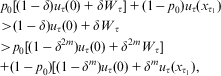 $$\matrix{{{p}_0}[(1\,{\rm{ - }}\,\delta ){{u}_\tau }(0)\, + \,\delta {{W}_\tau }]\, + \,(1\,{\rm{ - }}\,{{p}_0}){{u}_\tau }({{x}_{{{\tau }_1}}}) \cr \hskip-6pc \!\!\!\gt (1\,{\rm{ - }}\,\delta ){{u}_\tau }(0)\, + \,\delta {{W}_\tau } \cr \hskip-3pc \!\!\!\!\!\gt {{p}_0}[(1\,{\rm{ - }}\,{{\delta }^{2m}} ){{u}_\tau }(0)\, + \,{{\delta }^{2m}} {{W}_\tau }] \cr \!\!\!\!\!\!\!\!\!\!\!+ (1\,{\rm{ - }}\,{{p}_0})[(1\,{\rm{ - }}\,{{\delta }^m} ){{u}_\tau }(0)\, + \,{{\delta }^m} {{u}_\tau }({{x}_{{{\tau }_1}}}), \\ $$
where the second inequality above follows by setting j=m−1 in Inequality 15.
Phase 4.1. First, consider the choice of a type  $$${{\tau }_0}$$$
office holder. Following the above strategy, the politician chooses x = 0, is removed from office, and we move to Phase 4.2. Deviating to
 $$$x^{\prime} \, \notin \, \{ 0,{{x}_{{{\tau }_1}}}\} $$$
again leads to election of a challenger and Phase 4.2, so this cannot be profitable. If the politician deviates to
 $$$x^{\prime}\, = \,{{x}_{{{\tau }_1}}}$$$
, then she is re-elected and we remain in Phase 4.1, she then chooses x = 0, is removed from office, and we move to Phase 4.2. The office holder's expected discounted payoff is higher following the initial strategy and obtaining her ideal policy immediately before moving to Phase 4.2. Next, consider a type
 $$$\tau \ne {{\tau }_0}$$$
office holder. Following the above strategy, the politician chooses
 $$$x\, = \,{{x}_{{{\tau }_1}}}$$$
and is re-elected in every period. The best one-shot deviation is as in Phase 3, and it follows from Inequality 13 and the above arguments that one-shot deviations are unprofitable.
Now consider a type  $$$\tau \geq {{\tau }_1}$$$
voter. In case the incumbent chooses
 $$$x\, = \,{{x}_{{{\tau }_1}}}$$$
, then all voters’ beliefs are given by
 $$$\hat{p}$$$
. If the incumbent is re-elected, then she continues to choose
 $$$x\, = \,{{x}_{{{\tau }_1}}}$$$
and be re-elected. If the incumbent is removed from office, then we move to Phase 2(1). The expected discounted payoff from re-electing the incumbent exceeds that from electing a challenger if
 $$${{u}_\tau }({{x}_{{{\tau }_1}}})\, \gt \,{{V}_\tau }$$$
, which is implied by Inequality 15. In case the incumbent chooses
 $$$x \ne {{x}_{{{\tau }_1}}}$$$
, then all voters believe that with probability one the incumbent is type
 $$${{\tau }_0}$$$
. If the incumbent is re-elected, then we move to Phase 5, she chooses x = 0 and is removed from office, and we move to Phase 2(1). If the challenger is elected, then we move to Phase 4.2. By the arguments for Phase 3, the expected discounted payoff from electing the challenger exceeds that from re-electing the incumbent.
Phase 4.2. First, consider the choice of a type  $$${{\tau }_0}$$$
office holder. Following the above strategy, the politician chooses x = 0, is re-elected, and we move to Phase 4.0(1), where she alternately chooses
 $$$x\, = \,{{x}_{{{\tau }_1}}}$$$
for k periods and x = 0 for one period. If the politician deviates to
 $$$x^{\prime}\, = \,{{x}_{{{\tau }_1}}}$$$
, then she is re-elected, we move to Phase 4.1, she then chooses x = 0 and is removed from office, and we move to Phase 4.2. The one-shot deviation is unprofitable if
 $$\matrix {(1\,{\rm{ - }}\,\delta ){{u}_{{{\tau }_0}}}(0)\, + \,\delta {{W}_{{{\tau }_0}}}\, \gt \,(1\,{\rm{ - }}\,\delta ){{u}_{{{\tau }_0}}}({{x}_{{{\tau }_1}}})\, + \,(1\,{\rm{ - }}\,\delta )\delta {{u}_{{{\tau }_0}}}(0) \cr + \,{{\delta }^2} [{{p}_0}[(1\,{\rm{ - }}\,\delta ){{u}_{{{\tau }_0}}}(0)\, + \,\delta {{W}_{{{\tau }_0}}}]\, + \,(1\,{\rm{ - }}\,{{p}_0}){{u}_{{{\tau }_0}}}({{x}_{{{\tau }_1}}})] \\ $$
Using Inequality 14 and the arguments of Phase 3, the above inequality is implied by
 $$(1\,{\rm{ - }}\,{{\delta }^2} )[(1\,{\rm{ - }}\,\delta ){{u}_{{{\tau }_0}}}(0)\, + \,\delta {{W}_{{{\tau }_0}}}]\, \gt \,(1\,{\rm{ - }}\,\delta ){{u}_{{{\tau }_0}}}({{x}_{{{\tau }_1}}})\, + \,(1\,{\rm{ - }}\,\delta )\delta {{u}_{{{\tau }_0}}}(0).$$
Since  $$${{W}_{{{\tau }_0}}}\, \gt \,{{u}_{{{\tau }_0}}}({{x}_{{{\tau }_1}}})$$$
, this in turn holds if
 $$${{u}_{{{\tau }_0}}}(0)\, \gt \,{{u}_{{{\tau }_0}}}({{x}_{{{\tau }_1}}})$$$
, which holds by assumption. If the politician deviates to
 $$$x^{\prime} \, \notin \, \{ 0,{{x}_{{{\tau }_1}}}\} $$$
, then she is removed from office and we remain in Phase 4.2, which is not profitable. Next, consider a type
 $$$\tau \ne {{\tau }_0}$$$
office holder. Following the above strategy, the politician chooses
 $$$x\, = \,{{x}_{{{\tau }_1}}}$$$
and is re-elected in every period. The best one-shot deviation is as in Phase 3, and it follows from Inequality 13 and the above arguments that one-shot deviations are unprofitable.
Now consider a type  $$$\tau \,\geq \,{{\tau }_1}$$$
voter. In case the office holder chooses
 $$$x\, = \,{{x}_{{{\tau }_1}}}$$$
, then all voters’ beliefs are given by
 $$$\hat{p}$$$
. If the incumbent is re-elected, then she continues to choose
 $$$x\, = \,{{x}_{{{\tau }_1}}}$$$
and be re-elected. If the incumbent is removed from office, then we move to Phase 2(1), and again Inequality 15 implies that the voter's expected discounted payoff from re-electing the incumbent exceeds that from electing a challenger. In case the incumbent chooses x = 0, then all voters believe that with probability one the incumbent is type
 $$${{\tau }_0}$$$
. If the incumbent is re-elected, then we move to Phase 4.0(1), and if the incumbent is not re-elected, then we move to Phase 2(1). Again, Inequality 15 implies that the voter's expected discounted payoff from re-electing the incumbent exceeds that from electing a challenger. In case the office holder chooses
 $$$x \, \notin \, \{ 0,{{x}_{{{\tau }_1}}}\} $$$
, then all voters believe the incumbent is type
 $$${{\tau }_0}$$$
. If the incumbent is re-elected, then we move to Phase 5, she chooses x = 0, is removed from office, and we move to Phase 2(1). If the challenger is elected, then we remain in Phase 4.2. By the arguments for Phase 3, the expected discounted payoff from electing the challenger exceeds that from re-electing the incumbent.
Phase 5. Since the incumbent is always removed from office, it is optimal for office holder's of all types to choose their ideal policies. Now consider a type  $$$\tau \geq {{\tau }_1}$$$
voter. All voters believe that with probability one the incumbent is type
 $$${{\tau }_0}$$$
. If the incumbent is re-elected, then we remain in Phase 5, the politician chooses x = 0, is removed from office, and we move to Phase 2(1). If the challenger is elected, then we move directly to Phase 2(1). Thus the expected discounted payoff from electing the challenger exceeds that from re-electing the incumbent.
To conclude, for all ε > 0, we can choose  $$$a \in (0,{\epsilon})$$$
, natural number k, and
 $$$\hat{\delta } \in (0,1)$$$
such that for all
 $$$\delta \in (\hat{\delta },1)$$$
, there exists m such that Inequalities 5–7 and 12–14 are satisfied by a, δ, and β = δ m. Given these parameters, I have specified strategies and beliefs such that the policy a is chosen along the path of play by all types of office holder, voter beliefs satisfy Bayes’ rule along each office holder's personal path of play, and no politician has a profitable one-shot deviation, and such that all voter types vote as though pivotal. This completes Step 1.
An argument symmetric to that for Step 1 yields the next step of the proof.
Step 2: For all ε > 0, there exist  $$$b \in (1\,{\rm{ - }}\,{\epsilon},1)$$$
and
 $$$\hat{\delta } \in (0,1)$$$
such that for all
 $$$\delta \in (\hat{\delta },1)$$$
,
we have  $$${{{\bf {{x}}}}^b} \in P(\delta )$$$
.
Given the argument of Step 1, I do not provide the (redundant) details of Step 2. But it will be important to note that a and b can be chosen close enough to zero and one, respectively, to allow the same choice of k and m in both steps. To be more explicit, choose k such that for all  $$$\tau \ne {{\tau }_0}$$$
, Inequality 1 holds, and such that for all
 $$$\tau \ne {{\tau }_n}$$$
, the corresponding inequality for Step 2 holds. Choose
 $$$\overline{\beta } $$$
such that for all
 $$$\beta \in (0,\overline{\beta } )$$$
, Inequality 4 and the corresponding inequality for Step 2 hold, and such that there exists
 $$$\underline{\delta } \in (0,1)$$$
such that for all
 $$$\delta \in (\underline{\delta }, 1)$$$
and all
 $$$\beta \in (0,\overline{\beta } )$$$
, we have Inequality 5 for all
 $$$\tau \ne {{\tau }_0}$$$
and the corresponding inequality for Step 2 for all
 $$$\tau \ne {{\tau }_n}$$$
. Furthermore, define
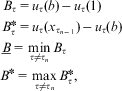 $$\matrix{ \!\!\!\!\!\!\!\!\!{{B}_\tau }\, = \,{{u}_\tau }(b)\,{\rm{ - }}\,{{u}_\tau }(1) \cr B_{\tau }^{\ast} \, = \,{{u}_\tau }({{x}_{{{\tau }_{n\,{\rm{ - }}\,1}}}})\,{\rm{ - }}\,{{u}_\tau }(b) \cr \!\!\!\!\!\!\!\!\!\!\!\!\!\!\!\!\!\!\!\!\!\!\!\!\!\underline{B} \, = \,\mathop {\min }\limits_{\tau \ne {{\tau }_n}} {{B}_\tau } \cr \!\!\!\!\!\!\!\!\!\!\!\!\!\!\!\!\!\!\!\!\!{{B}^\ast} \, = \,\mathop {\max }\limits_{\tau \ne {{\tau }_n}} B_{\tau }^{\ast}, \\ $$
and note that by the arguments in Step 1, we have
 $$\mathop {\lim }\limits_{b \uparrow 1} \left( {\frac{{{{u}_{{{\tau }_n}}}(1)\,{\rm{ - }}\,{{u}_{{{\tau }_n}}}(b)}}{{{{u}_{{{\tau }_n}}}(b)\,{\rm{ - }}\,{{u}_{{{\tau }_n}}}({{x}_{{{\tau }_{n\,{\rm{ - }}\,1}}}})}}} \right)\left( {\frac{{{{B}^\ast} }}{{\underline{B} }}} \right)\, = \,0.$$
Thus we can choose  $$$a \in (0,{\epsilon})$$$
,
 $$$b \in (1\,{\rm{ - }}\,{\epsilon},1)$$$
and
 $$$\beta \in (0,\overline{\beta } )$$$
such that Inequalities 10 and 11 hold, along with the corresponding inequalities for Step 2. Then the arguments in Step 1 allow us to specify
 $$$\hat{\delta } \in (\underline{\delta }, 1)$$$
so that for all
 $$$\delta \in (\hat{\delta },1)$$$
, there exists m such that Inequalities 12–14 hold, along with the corresponding inequalities for Step 2. This permits the equilibrium construction from Step 1 to be applied in Step 2 with the same choice of k and m.
Next I define a procedure for splicing the equilibria from Steps 1 and 2 to produce a path of policies that alternates between a and b, and I use the construction recursively to generate paths that cycle between the alternatives to approximate any empirical frequency.
Step 3: For all ε > 0, there exist  $$$a \in (0,{\epsilon})$$$
and
 $$$b \in (1\,{\rm{ - }}\,{\epsilon},1)$$$
such that for all natural numbers ℓ and all k with
 $$$k = 0,1, \ldots {{,2}^\ell } $$$
, there exists
 $$$\tilde{\delta } \in (0,1)$$$
such that for all
 $$$ \delta \in (\tilde{\delta },1) $$$
, there exists
 $$$ {\bf {{x}}} \in P(\delta ) $$$
such that in consecutive runs of
 $$$ {{2}^\ell } $$$
periods, the path x visits a for k periods and b for
 $$${{2}^\ell } \,{\rm{ - }}\,k$$$
periods; that is, for all
 $$$ m = 0,1,2, \ldots $$$
,
 $$\matrix{ \!\!\!\!\!\!\!\!\!\!\!\!\!\!\# \{ t|m{{2}^\ell } + 1\,\leq \,t\,\leq \,(m\, + \,{{1)2}^\ell } \:\;{\rm and}\;\:{{x}_t}\, = \,a\} \, = \,k \cr \# \{ t|m{{2}^\ell } \, + \,1\,\leq \,t\,\leq \,(m\, + \,{{1)2}^\ell } \:\;{\rm and}\;\:{{x}_t}\, = \,b\} \, = \,{{2}^\ell } \,{\rm{ - }}\,k. \\ $$
The proof is by induction. Fix ε > 0. By Step 1, there exist  $$$a \in (0,{\epsilon})$$$
and
 $$$\delta ^{\prime}\, \lt \,1$$$
such that for all
 $$$\delta \in (\delta ^{\prime},1)$$$
, we have
 $$${{{\bf {{x}}}}^a} \in P(\delta )$$$
. Similarly, by Step 2, there exist
 $$$b \in (1\,{\rm{ - }}\,{\epsilon},1)$$$
and
 $$$\delta ^{\prime\prime}\, \lt \,1$$$
such that for all
 $$$\delta \in (\delta ^{\prime\prime},1)$$$
, we have
 $$${{{\bf {{x}}}}^b} \in P(\delta )$$$
. For the basis step, consider ℓ = 1. For k = 0 and k = 2, the desired result follows from Steps 2 and 1, respectively. Consider k = 1, and set
 $$${\bf {{x}}} = (b,a,b,a, \ldots )$$$
. I focus on the former case without loss of generality. Set
 $$$\tilde{\delta } = \sqrt {\max \{ \delta ^{\prime},\delta ^{\prime \prime}\} } $$$
, choose
 $$$\delta \in (\tilde{\delta },1)$$$
, and define strategies and beliefs by ‘splicing’ the specifications in Steps 1 and 2. That is, we specify actions and beliefs according to the equilibrium from Step 1 in odd periods and using the equilibrium from Step 2 in even periods.
To be more precise, we begin in Phase 1 in both odd and even periods, so that the path of play from the initial history is the sequence  $$$(a,b,a,b, \ldots )$$$
, and we specify strategies from Step 1 in odd periods and from Step 2 in even periods. Following any deviation in an odd period t, for example, the transition between phases in subsequent odd periods follows the protocol from Step 1 (applied to odd periods), and we specify that the phase transitions in the next even period t+1 as though an analogous deviation had occurred in period t − 1; from that point on, the transition between phases in even periods follows the protocol from Step 2 (applied to even periods). So, if along the equilibrium path the office holder deviates to
 $$$x^{\prime} \ne a$$$
in an odd period t, then the politician is removed from office, and we move to Phase 2(1) for the next m even periods (with actions determined by Step 2) and for the next m odd periods (with actions determined by Step 1). After that span of 2 m periods has elapsed, we move to Phase 3 for the next m even periods and for the next m odd periods. We then enter Phase 4.0 or Phase 4.1, depending on policy choices in odd and even periods. Subsequent deviations are treated the same way. Suppose in an odd period t′, we are in Phase 3, and the office holder chooses
 $$$x^{\prime} \, \notin \, \{ 0,{{x}_{{{\tau }_1}}}\} $$$
and is not re-elected. Then we transition to Phase 4.2 in the next even period t′+1 and the next odd period t′+2. If the newly elected office holder is type
 $$${{\tau }_n}$$$
, for example, then she chooses
 $$$x\, = \,{{x}_{{{\tau }_n}}}$$$
in period t′+1, we transition to Phase 4.0 in all subsequent even periods, she chooses
 $$$x\, = \,{{x}_{{{\tau }_1}}}$$$
in period t′+2, and we transition to Phase 4.1 in all subsequent odd periods. On the other hand, if the new office holder is type
 $$$\tau $$$
with
 $$${{\tau }_1}\,\leq \,\tau \,\leq \,{{\tau }_{n\,{\rm{ - }}\,1}}$$$
, then she chooses
 $$${{x}_{{{\tau }_{n\,{\rm{ - }}\,1}}}}$$$
in period t′+1 and
 $$${{x}_{{{\tau }_1}}}$$$
in period t′+2, and we transition to Phase 4.1 in all subsequent periods.
Policy and voting choices are given by the strategies from Steps 1 and 2, although now we must take care in specifying voter beliefs when we enter Phase 5 and when information is revealed in Phases 3(1) and 4.2. To simplify exposition, we focus on the case in which the transition first occurs in an odd period, so that information is revealed to voters in the next even period. First, note that Phase 5 is entered only off a politician's personal path of play and only when she is re-elected, so that voter beliefs may be specified arbitrarily. Let  $$$\overline{x} \in \{ 0,1\} $$$
be the policy that is weakly preferred among {0,1} by a majority of voters, and let
 $$$\underline{x} \in \{ 0,1\} $$$
be the remaining policy, so that
 $$ \mathop{\sum} \{ {{q}_j}|{{u}_{{{\tau }_j}}}(\overline{x} )\geq {{u}_{{{\tau }_j}}}(\underline{x} )\} \geq \frac{1}{2}. $$
Thus by concavity, the policy x is the worst possible policy for a majority of voters. Let  $$$\underline{\tau } \in \{ {{\tau }_0},{{\tau }_n}\} $$$
be the type such that
 $$${{x}_{\underline{\tau } }}\, = \,\underline{x} $$$
. In Phase 5, whether in an odd or even period, we specify that voters believe with probability one that the office holder is type
 $$$\underline {\tau} $$$
. This ensures that a majority of voters prefers to replace the incumbent with a challenger, as dictated in Steps 1 and 2.
Second, after entering Phase 3(1) in an odd period t, if the office holder chooses x = 0, then voters believe that with probability one the office holder is type  $$${{\tau }_0}$$$
, and if she is re-elected, then we move to Phase 3(1) in the following even period t+1. As noted in footnote 10, the information revealed by this choice does not affect the incentives of type
 $$$\tau \ne {{\tau }_n}$$$
voters to re-elect the incumbent prior to period t+1. If the office holder chooses
 $$$x\, = \,{{x}_{{{\tau }_1}}}$$$
, then voters’ beliefs are given by the posterior
 $$$\hat{p}$$$
conditional on the office holder's type belonging to
 $$$\{ {{\tau }_1}, \ldots, {{\tau }_n}\} $$$
, and if she is re-elected, then we move to Phase 3(1) in the following even period. As noted in footnote 9, this revelation of information does not affect the incentives of voters to re-elect the incumbent. If the office holder chooses
 $$$x \, \notin \, \{ 0,{{x}_{{{\tau }_1}}}\} $$$
, then voters believe she is type
 $$$\underline {\tau }$$$
, and if she is re-elected, then we move to Phase 5; thus, the office holder will be removed from office, as required. Supposing the incumbent is re-elected in period t, voter beliefs are updated in period t+1 and phases transition as follows. If voter beliefs are that the incumbent is type
 $$${{\tau }_0}$$$
and she chooses
 $$$x\, = \,{{x}_{{{\tau }_{n\,{\rm{ - }}\,1}}}}$$$
in period t+1, then beliefs are unchanged, and if she is re-elected, then we move to Phase 3(2) in the next odd period t+2; again, footnote 10 implies that the incumbent will be re-elected. If voter beliefs are that the incumbent is type
 $$${{\tau }_0}$$$
and she chooses x = 1, then voters believe she is type
 $$$\underline {\tau }$$$
, and if she is re-elected, then we move to Phase 5, and she is removed from office. If voter beliefs are
 $$$\hat{p}$$$
and she chooses
 $$$x\, = \,{{x}_{{{\tau }_{n\,{\rm{ - }}\,1}}}}$$$
, then voter beliefs are given by the posterior conditional on the office holder's type belonging to
 $$$\{ {{\tau }_1}, \ldots, {{\tau }_{n - 1}}\} $$$
, and if she is re-elected, then we move to Phase 3(2) in the next odd period t+2; and if voter beliefs are
 $$$\hat{p}$$$
and the incumbent chooses x = 1, then voters believe she is type
 $$${{\tau }_n}$$$
, and if she is re-elected, then we move to Phase 3(2). Again, footnote 9 implies that the incumbent will be re-elected following either choice. And if the office holder chooses
 $$$x \, \notin \, \{ {{x}_{{{\tau }_{n - 1}}}},1\} $$$
, then voters believe she is type
 $$$\underline {\tau }$$$
, and the politician is removed from office. Supposing the incumbent is re-elected in t+1, voter beliefs are again given by Bayes’ rule, as applicable.
Third, after entering Phase 4.2 in an odd period t, if the office holder chooses x = 0, then voters believe that with probability one the office holder is type  $$${{\tau }_0}$$$
, and if she is re-elected, then we move to Phase 4.2 in the following even period period t+1. If the office holder chooses
 $$$x\, = \,{{x}_{{{\tau }_1}}}$$$
, then voter beliefs are given by
 $$$\hat{p}$$$
, and if she is re-elected, then we also move to Phase 4.2 in the following even period t+1. Again, in either case, type
 $$$\tau \,\geq \,{{\tau }_1}$$$
voters will avoid transitioning to Phase 2(1) by re-electing the incumbent in period t. Then voter beliefs are updated in period t+1 and phases transition as follows. If voter beliefs are that the incumbent is type
 $$${{\tau }_0}$$$
and she chooses
 $$$x\, = \,{{x}_{{{\tau }_{n\,{\rm{ - }}\,1}}}}$$$
in period t+1, then beliefs are unchanged, and when she is re-elected, we move to Phase 4.0 in all subsequent odd periods and to Phase 4.1 in all subsequent even periods, until a further deviation occurs. If voter beliefs are that the incumbent is type
 $$${{\tau }_0}$$$
and she chooses x = 1, then voters believe she is type
 $$$\underline\tau $$$
, and if she is re-elected, then we move to Phase 5, and she is removed from office. If voter beliefs are
 $$$\hat{p}$$$
and she chooses
 $$$x\, = \,{{x}_{{{\tau }_{n\,{\rm{ - }}\,1}}}}$$$
, then voter beliefs are given by the posterior conditional on the office holder's type belonging to
 $$$\{ {{\tau }_1}, \ldots, {{\tau }_{n\,{\rm{ - }}\,1}}\} $$$
, and when she is re-elected, we move to Phase 4.1 in all subsequent odd periods and to Phase 4.0 in all subsequent even periods, until a further deviation occurs. If voter beliefs are
 $$$\hat{p}$$$
and she chooses x = 1, then voters believe that she is type
 $$${{\tau }_n}$$$
, and when she is re-elected, we move to Phase 4.1 in all subsequent odd periods and to Phase 4.0 in all subsequent even periods. And if the office holder chooses
 $$$x \, \notin \, \{ {{x}_{{{\tau }_{n\,{\rm{ - }}\,1}}}},1\} $$$
, then voters believe she is type
 $$$\underline {\tau }$$$
, and she is removed from office. Supposing the incumbent is re-elected in t+1, voter beliefs are again updated via Bayes’ rule, as applicable.
In effect, this splicing of strategies punishes a deviation in an odd period t by following the punishments from Step 1 in all future odd periods, and by following Step 2 in all future even periods, simulating punishments as though an analogous deviation had occurred in the previous even period t − 1. A similar construction is used following a deviation in an even period. This establishes a perfect Bayesian electoral equilibrium with path of play  $$$(a,b,a,b, \ldots )$$$
and provides a splicing procedure that can be iterated generally.
For the induction step, assume the claim is true for ℓ − 1, choose any  $$$k\, = \,0,1, \ldots {{,2}^\ell } $$$
, and write
 $$$k\, = \,k^{\prime}\, + \,k^{\prime\prime}$$$
, where
 $$$k^{\prime},k^{\prime\prime}\leq {{2}^{\ell \,{\rm{ - }}\,1}} $$$
. By the induction hypothesis, there exists
 $$$\delta ^{\prime} \in (0,1)$$$
such that for all
 $$$\delta \in (\delta ^{\prime},1)$$$
, there exists
 $$${\bf {{y}}} \in P(\delta )$$$
such that for all
 $$$m = 0,1,2, \ldots $$$
,
 $$\matrix{ \!\!\!\!\!\!\!\!\!\!\!\!\!\# \{ t|m{{2}^{\ell \,{\rm{ - }}\,1}} \, + \,1\,\leq \,t\,\leq \,(m\, + \,{{1)2}^{\ell \,{\rm{ - }}\,1}} \;{\rm and}\;\:{{y}_t}\, = \,a\} \, = \,k^{\prime} \cr \# \{ t|m{{2}^{\ell \,{\rm{ - }}\,1}} \, + \,1\,\leq \,t\,\leq \,(m\, + \,{{1)2}^{\ell \,{\rm{ - }}\,1}} \:\;{\rm and}\;\:{{y}_t}\, = \,b\} \, = \,{{2}^\ell } \,{\rm{ - }}\,k^{\prime}. \\ $$
And there exists  $$$\delta ^{\prime\prime} \in (0,1)$$$
such that for all
 $$$\delta \in (\delta ^{\prime\prime},1)$$$
, there exists
 $$${\bf {{z}}} \in P(\delta )$$$
such that for all
 $$$m\, = \,0,1,2, \ldots $$$
,
 $$\matrix {\!\!\!\!\!\!\!\!\!\!\!\!\!\# \{ t|m{{2}^{\ell \,{\rm{ - }}\,1}} \, + \,1\leq t\leq (m\, + \,{{1)2}^{\ell \,{\rm{ - }}\,1}} \:\;{\rm and}\;\:{{z}_t}\, = \,a\} \, = \,k^{\prime\prime} \cr \# \{ t|m{{2}^{\ell \,{\rm{ - }}\,1}} \, + \,1\leq t\leq (m\, + \,{{1)2}^{\ell \,{\rm{ - }}\,1}} \:\;{\rm and}\;\:{{z}_t}\, = \,b\} \, = \,{{2}^\ell } \,{\rm{ - }}\,k^{\prime\prime}. \\ $$
We then set  $$$\tilde{\delta }\, = \,\sqrt {\max \{ \delta ^{\prime},\delta ^{\prime\prime}\} } $$$
, and for every
 $$$\delta \, \gt \,\tilde{\delta }$$$
, we splice the equilibria supporting paths x and y according to the above procedure. This yields a perfect Bayesian electoral equilibrium that generates the path
 $$${\bf {{x}}}\, = \,({{x}_1},{{x}_2}, \ldots )\, = \,({{y}_1},{{z}_1},{{y}_2},{{z}_2}, \ldots )$$$
from the initial history. Formally, we define x by
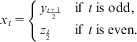 $${{x}_t}\, = \,\left\{ \matrix {{{{y}_{\frac{{t\, + \,1}}{2}}}} \hfill &#x0026; {\:{\rm if}\;t{\rm \;is\;odd},\thinsp} \hfill \cr {{{z}_{\frac{t}{2}}}} \hfill &#x0026; {\:{\rm if}\;t{\rm \;is\;even}.\:} \hfill \\$$
Then for all  $$$m\, = \,0,1,2, \ldots $$$
, we have
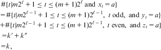 $$\matrix{ \hskip-5pc \! \# \{ t|m{{2}^\ell } \, + \,1\leq t\leq (m\, + \,{{1)2}^\ell } \:\;{\rm and}\;\:{{x}_t}\, = \,a\} \cr = \# \{ t|m{{2}^{\ell \,{\rm{ - }}\,1}} \, + \,1\leq t\leq (m\, + \,{{1)2}^{\ell \,{\rm{ - }}\,1}}, \:\;t\;{\rm odd},\;{\rm and}\;{{y}_t}\, = \,a\:\} \cr + \# \{ t|m{{2}^{\ell \,{\rm{ - }}\,1}} \, + \,1\leq t\leq (m\, + \,{{1)2}^{\ell \,{\rm{ - }}\,1}}, \:\;t\;{\rm even},\;{\rm and}\;{{z}_t}\, = \,a\:\} \cr \hskip-16pc \ \!\! = k^{\prime}\, + \,k^{\prime\prime} \cr \hskip-18pc = k, \\ $$
where the first equality follows by noting that when t (odd) ranges from  $$$m{{2}^\ell } \, + \,1$$$
to
 $$$(m\, + \,{{1)2}^\ell } \,{\rm{ - }}\,1$$$
, the ratio
 $$$\frac{{t\, + \,1}}{2}$$$
ranges from
 $$$m{{2}^{\ell \,{\rm{ - }}\,1}} \, + \,1$$$
to
 $$$(m\, + \,{{1)2}^{\ell \,{\rm{ - }}\,1}} $$$
, and similarly, when t (even) ranges from
 $$$m{{2}^\ell } \, + \,2$$$
to
 $$$(m\, + \,{{1)2}^\ell } $$$
, the ratio
 $$$\frac{t}{2}$$$
ranges from
 $$$m{{2}^{\ell \,{\rm{ - }}\,1}} \, + \,1$$$
to
 $$$(m\, + \,{{1)2}^{\ell \,{\rm{ - }}\,1}} $$$
. This establishes the desired perfect Bayesian equilibrium.
The final step of the proof uses the equilibria from Step 3 to punish deviations from arbitrary paths through a region of the policy space that becomes arbitrarily large as citizens become patient.
Step 4: For all  $$$a,b \in X$$$
, with
 $$$0\, \lt \,a\, \lt \,b\, \lt \,1$$$
, there exists
 $$$\overline{\delta } \in (0,1)$$$
such that for all
 $$$\delta \in (\overline{\delta }, 1)$$$
, we have
 $$${{[a,b]}^\infty } \subseteq P(\delta )$$$
.
Consider  $$$a,b \in X$$$
with
 $$$0\, \lt \,a\, \lt \,b\, \lt \,1$$$
. Fix
 $$${\epsilon}\, = \,\frac{1}{2}\min \{ a,1\,{\rm{ - }}\,b\} $$$
, and let
 $$$a^{\prime} \in (0,{\epsilon})$$$
and
 $$$b^{\prime} \in (1\,{\rm{ - }}\,{\epsilon},1)$$$
be as in Step 3. For each
 $$$x \in [a,b]$$$
, we can write
 $$$x\, = \,\alpha (x)a^{\prime}\, + \,(1\,{\rm{ - }}\,\alpha (x))b^{\prime}$$$
, where
 $$\alpha (x)\, = \,\frac{{b^{\prime}\,{\rm{ - }}\,x}}{{b^{\prime}\,{\rm{ - }}\,a^{\prime}}},$$
and then we have
 $$0\,\, \lt \,\,\frac{{b^{\prime}\,{\rm{ - }}\,b}}{{b^{\prime}\,{\rm{ - }}\,a^{\prime}}}\,\,\leq \,\,\alpha (x)\,\,\leq \,\,\frac{{b^{\prime}\,{\rm{ - }}\,a}}{{b^{\prime}\,{\rm{ - }}\,a^{\prime}}}\,\, \lt \,\,1.$$
Since each  $$${{u}_\tau }$$$
is strictly concave, it follows that for all
 $$$x \in [a,b]$$$
, we have
 $$${{u}_\tau }(x)\, \gt \,\alpha (x){{u}_\tau }(a^{\prime})\, + \,(1\,{\rm{ - }}\,\alpha (x)){{u}_\tau }(b^{\prime})$$$
. More generally, let Λ denote the set of probability measures λ with support contained in [a, b], and note that for all λ ∈ Λ, we have
 $$\matrix{ \int {{u}_\tau }(x)\lambda (dx) \gt \int [\alpha (x){{u}_\tau }(a^{\prime})\, + \,(1\,{\rm{ - }}\,\alpha (x)){{u}_\tau }(b^{\prime})]\lambda (dx) \cr \hskip-5pc= \alpha (E[\lambda ]){{u}_\tau }(a^{\prime})\, + \,(1\,{\rm{ - }}\,\alpha (E[\lambda ])){{u}_\tau }(b^{\prime}). \\ $$
Therefore, since  $$${{u}_\tau }$$$
is continuous and Λ is compact in the weak* topology, we have
 $$\mathop {\min }\limits_{\lambda \in \Lambda } \left[ {\int {{u}_\tau }(x)\lambda (dx)\,{\rm{ - }}\,\alpha (E[\lambda ]){{u}_\tau }(a^{\prime})\,{\rm{ - }}\,(1\,{\rm{ - }}\,\alpha (E[\lambda ])){{u}_\tau }(b^{\prime})} \right] \equiv \eta \, \gt \,0.$$
For all λ ∈ Λ, we can approximate α(E[λ]) by  $$$\frac{k}{{{{2}^\ell } }}$$$
through choice of the natural numbers ℓ and
 $$$k\, = \,0,1, \ldots {{,2}^\ell } $$$
. Thus, there exist k and ℓ such that
 $$\int {{u}_\tau }(x)\lambda (dx)\, \gt \,\left( {\frac{k}{{{{2}^\ell } }}} \right){{u}_\tau }(a^{\prime})\, + \,\left( {1\,{\rm{ - }}\,\frac{k}{{{{2}^\ell } }}} \right){{u}_\tau }(b^{\prime})\, + \,\frac{\eta }{2}.$$
Define Λk,ℓ as the set of probability measures λ ∈ Λ such that Inequality 16 holds. It follows that  $$${{\{ {{\Lambda }^{k,\ell }} \} }_{k,\ell }}$$$
is an open covering of Λ, and since the latter set is compact, it possesses a finite subcover. Let F be a finite set of (k, ℓ) pairs, with ℓ a natural number and
 $$$k \in \{ 0,1,2, \ldots {{,2}^\ell } \} $$$
, such that
 $$$\Lambda \subseteq \bigcup\nolimits_{(k,\ell ) \in F} {{\Lambda }^{k,\ell }} $$$
. By repeated application of Step 3, we can choose
 $$$\tilde{\delta } \in (0,1)$$$
such that for all
 $$$\delta \in (\tilde{\delta },1)$$$
and all
 $$$(k,\ell ) \in F$$$
, there exists
 $$${{{\bf {{x}}}}^{k,\ell }} \in P(\delta )$$$
such that for all
 $$$m = 0,1,2, \ldots $$$
,
 $$\matrix {\!\!\!\!\!\!\!\!\!\!\!\!\!\# \{ t|m{{2}^\ell } \, + \,1\,\leq \,t\,\leq \,(m\, + \,{{1)2}^\ell } \:\;{\rm and}\;\:{{x}_t}\, = \,a^{\prime}\} \, = \,k \cr \# \{ t|m{{2}^\ell } \, + \,1\,\leq \,t\,\leq \,(m\, + \,{{1)2}^\ell } \:\;{\rm and}\;\:{{x}_t}\, = \,b^{\prime}\} \, = \,{{2}^\ell } \,{\rm{ - }}\,k. \\ $$
Given any pair (k, ℓ), discount factor δ < 1, and type  $$$\tau $$$
, the discounted sum of utility from
 $$${{{\bf {{x}}}}^{k,\ell }} $$$
, denoted
 $$$U_{\tau }^{{k,\ell }} $$$
, satisfies
 $$ U_{\tau }^{{k,\ell }} \, = \,\mathop{\sum}\limits_{t\, = \,1}^{{{2}^\ell } } {{\delta }^{t\,{\rm{ - }}\,1}} [{{I}_{a^{\prime}}}(x_{t}^{{k,\ell }} ){{u}_\tau }(a^{\prime})\, + \,{{I}_{b^{\prime}}}(x_{t}^{{k,\ell }} ){{u}_\tau }(b^{\prime})]\, + \,{{\delta }^{{{2}^\ell } }} U_{\tau }^{{k,\ell }}, $$
and therefore, after normalizing by (1 − δ), we have
 $$(1\,{\rm{ - }}\,\delta )U_{\tau }^{{k,\ell }} = \frac{{1\,{\rm{ - }}\,\delta }}{{1\,{\rm{ - }}\,{{\delta }^{{{2}^\ell } }} }}\mathop{\sum}\limits_{t\, = \,1}^{{{2}^\ell } } {{\delta }^{t\,{\rm{ - }}\,1}} [{{I}_{a^{\prime}}}(x_{t}^{{k,\ell }} ){{u}_\tau }(a^{\prime})\, + \,{{I}_{b^{\prime}}}(x_{t}^{{k,\ell }} ){{u}_\tau }(b^{\prime})],$$
where  $$${{I}_{a^{\prime}}}$$$
and
 $$${{I}_{b^{\prime}}}$$$
are the indicator functions for a′ and b′. Taking the limit as δ goes to one and applying l'Hôpital's rule, we have
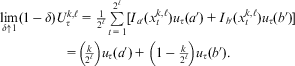 $$\matrix{ \mathop {\lim }\limits_{\delta \uparrow 1} (1\,{\rm{ - }}\,\delta )U_{\tau }^{{k,\ell }} \, = \,\frac{1}{{{{2}^\ell } }}\mathop{\sum}\limits_{t\, = \,1}^{{{2}^\ell } } [{{I}_{a^{\prime}}}(x_{t}^{{k,\ell }} ){{u}_\tau }(a^{\prime})\, + \,{{I}_{b^{\prime}}}(x_{t}^{{k,\ell }} ){{u}_\tau }(b^{\prime})] \cr = \left( {\frac{k}{{{{2}^\ell } }}} \right){{u}_\tau }(a^{\prime})\, + \,\left( {1\,{\rm{ - }}\,\frac{k}{{{{2}^\ell } }}} \right){{u}_\tau }(b^{\prime}). \\ $$
Now let Λδ consist of all probability measures λ ∈ Λ such that for some  $$$(k,\ell ) \in F$$$
, we have
 $$\int {{u}_\tau }(x)\lambda (dx)\, \gt \,(1\,{\rm{ - }}\,\delta )U_{\tau }^{{k,\ell }} \, + \,\frac{\eta }{4}.$$
Since  $$$\Lambda \subseteq \bigcup\nolimits_{(k,\ell ) \in F} {{\Lambda }^{k,\ell }} $$$
and
 $$$(1\,{\rm{ - }}\,\delta )U_{\tau }^{{k,\ell }} \rightarrow \left( {\frac{k}{{{{2}^\ell } }}} \right){{u}_\tau }(a^{\prime})\, + \,\left( {1\,{\rm{ - }}\,\frac{k}{{{{2}^\ell } }}} \right){{u}_\tau }(b^{\prime})$$$
, it follows from Inequality 16 that for each λ ∈ Λ, we have
 $$$\lambda \in {{\Lambda }^\delta } $$$
for δ sufficiently close to one. That is,
 $$$\{ {{\Lambda }^\delta } |\delta \in (0,1)\} $$$
is an open covering of Λ. Again, since Λ is compact, this collection possesses a finite subcover, indexed by a finite set
 $$$D \subseteq (0,1)$$$
. Therefore, setting
 $$$\delta ^{\prime}\, = \,\max D\, \lt \,1$$$
, it follows that for all
 $$$\delta \in (\delta ^{\prime},1)$$$
and all
 $$$\lambda \in \Lambda $$$
, there exists
 $$$(k,\ell ) \in F$$$
such that Inequality 17 holds. Furthermore, choose
 $$$\overline{\delta } \in (\delta ^{\prime},1)$$$
such that
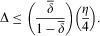 $$\rDelta \leq \left( {\frac{{\overline{\delta } }}{{1\,{\rm{ - }}\,\overline{\delta } }}} \right)\left( {\frac{\eta }{4}} \right).$$
Finally, consider any  $$$\delta \in (\overline{\delta }, 1)$$$
and any
 $$${\bf {{x}}} \in {{[a,b]}^\infty } $$$
. I specify a perfect Bayesian equilibrium that generates x from the initial history by again defining actions and beliefs in each of a number of phases and by specifying a rule for transitioning between phases. Now, however, the procedure is simpler. Phase 0 will represent the path of play from the initial history, while a countable number of phases,
 $$$t = 1,2, \ldots $$$
, are used as punishments. Specifically, Phase t is used to punish deviations from Phase 0 in period t, while further deviations from phase t are handled implicitly in Step 3. Note that for each t, we can write the discounted utility of a type
 $$$\tau $$$
citizen from
 $$$({{x}_t},{{x}_{t + 1}},{{x}_{t + 2}}, \ldots )$$$
as the integral with respect to a probability measure
 $$${{\lambda }_t} \in \rLambda $$$
; that is,
 $$\mathop{\sum}\limits_{t^{\prime}\, = \,t}^\infty {{\delta }^{t^{\prime}\,{\rm{ - }}\,t}} {{u}_\tau }({{x}_{t^{\prime}}})\, = \,\frac{1}{{1\,{\rm{ - }}\,\delta }}\int {{u}_\tau }(x){{\lambda }_t}(dx),$$
where λt is defined by
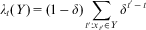 $${{\lambda }_t}(Y)\, = \,(1\,{\rm{ - }}\,\delta )\mathop{\sum}\limits_{t^{\prime}:{{x}_{t^{\prime}}} \in Y} {{\delta }^{t^{\prime}\,{\rm{ - }}\,t}} $$
for all measurable  $$$Y \subseteq [0,1]$$$
. It follows that there exists
 $$$(k,\ell ) \in F$$$
such that Inequality 17 holds with λ = λt. To define the equilibrium, we specify that in period t of Phase 0, all types of office holder choose xt, and voters’ beliefs along the path of play are given by the prior p, and all voter types vote to re-elect the incumbent. If the office holder chooses
 $$$x^{\prime} \ne {{x}_t}$$$
, then voter beliefs are again given by the prior. In Phase
 $$$t\, = \,1,2, \ldots $$$
, let
 $$$(k,\ell ) \in F$$$
satisfy Inequality 17 with λ = λt +1, and use Step 3 to specify strategies and beliefs so that they form a perfect Bayesian electoral equilibrium that generates the path
 $$${{{\bf {{x}}}}^{k,\ell }} $$$
beginning in period t+1; that is, the path beginning in period t+1 is
 $$$(x_{1}^{{k,\ell }}, x_{2}^{{k,\ell }}, \ldots )$$$
. The initial history is labeled Phase 0, and in period t of Phase 0, if it is not the case that the office holder chooses xt and is re-elected, then transition to the punishment Phase t+1 occurs in the next period t+1.
To verify that this specification constitutes a perfect Bayesian electoral equilibrium, note that the discounted payoff to a type  $$$\tau $$$
citizen from a one-shot deviation in period t of Phase 0 is bounded above by
 $$${\max }_{x \in X} {{u}_\tau }(x) + \delta U_{\tau }^{{k,\ell }} $$$
. Furthermore,
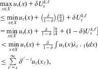 $$\matrix{\mathop {\max }\limits_{x \in X} {{u}_\tau }(x)\, + \,\delta U_{\tau }^{{k,\ell }} \hfill \cr \leq \mathop {\min }\limits_{x \in X} {{u}_\tau }(x)\, + \,\left( {\frac{\delta }{{1\,{\rm{ - }}\,\delta }}} \right)\left( {\frac{\eta }{4}} \right)\, + \,\delta U_{\tau }^{{k,\ell }} \hfill \cr = \mathop {\min }\limits_{x \in X} {{u}_\tau }(x)\, + \,\frac{\delta }{{1\,{\rm{ - }}\,\delta }}\left[ {\frac{\eta }{4}\, + \,(1\,{\rm{ - }}\,\delta )U_{\tau }^{{k,\ell }} } \right] \hfill \cr \!\lt \mathop {\min }\limits_{x \in X} {{u}_\tau }(x)\, + \,\frac{\delta }{{1\,{\rm{ - }}\,\delta }}\int {{u}_\tau }(x){{\lambda }_{t\, + \,1}}(dx) \cr \!\!\!\!\!\!\!\!\!\!\!\!\!\!\!\!\!\!\!\!\!\!\!\!\!\!\!\!\!\!\!\!\!\!\!\!\!\!\!\!\!\!\!\leq \mathop{\sum}\limits_{t^{\prime}\, = \,t}^\infty {{\delta }^{t^{\prime}\,{\rm{ - }}\,t}} {{u}_\tau }({{x}_{t^{\prime}}}), \\ $$
where the inequalities follow from 18, 17 and 19, respectively. Therefore, one-shot deviations are unprofitable, and we conclude that there exists a perfect Bayesian equilibrium that generates the path x from the initial history.



