1. Introduction
The binary droplet collision is a frequently observed phenomenon in a variety of natural and technical processes, for example in the evolution of raindrops, in spray processes such as fuel spray in internal combustion, spray painting and agricultural sprays. The outcomes of binary droplet collisions affect the droplet size distribution in spray processes. In previous studies (Ashgriz & Poo Reference Ashgriz and Poo1990; Jiang, Umemura & Law Reference Jiang, Umemura and Law1992; Qian & Law Reference Qian and Law1997), which focused on droplet collisions at low collision energy, distinct regimes of collision outcomes have been observed and characterized. It is well accepted that the collision outcomes for two identical droplets are dominated by the Weber number, which is defined as
 $We={\it\rho}U_{r}^{2}D_{0}/{\it\sigma}$
, where
 ${\it\rho}$
is the density,
 $U_{r}$
the relative velocity,
 $D_{0}$
the initial droplet diameter and
 ${\it\sigma}$
the surface tension of the fluid, and by the impact parameter
 $B=b/D_{0}$
, which is defined as the ratio of the offset of the trajectories of the droplets to the droplet diameter. In the regime of low Weber numbers (of the order of 10), four different collision outcomes are identified depending on the combination of
 $We$
and
 $B$
, namely (1) coalescence, (2) bouncing, (3) reflexive separation and (4) stretching separation.
In multinozzle sprays generated in devices like liquid rocket engines and in food processing (Roth, Rieber & Frohn Reference Roth, Rieber and Frohn1999), droplet collision at high Weber numbers occurs, which results in significantly different phenomena. Roth et al. (Reference Roth, Rieber and Frohn1999) conducted experimental studies on head-on binary collisions of isopropanol droplets at Weber numbers ranging from 1030 to 2876. Their results show that with increasing Weber number, the rim of the collision complex becomes increasingly unstable. If the Weber number is high enough, secondary droplets are splattered out from the rim of the collision complex. They also conducted numerical simulations, but only qualitatively at relatively low Weber numbers due to the large computational effort required as a result of the extremely high collision energy. Despite the lower Weber number in their numerical simulations, the instability of the rim is too strong compared to the experimental results. Pan, Chou & Tseng (Reference Pan, Chou and Tseng2009) conducted an experimental study of head-on binary droplet collisions at Weber numbers up to about 5000. They presented clear images for the deformation history of water collision complexes. Their results show that the instability of the rim of the water collision complex emerges at much smaller Weber numbers compared to isopropanol droplets. Recently, Kuan, Pan & Shyy (Reference Kuan, Pan and Shyy2014) conducted a numerical study of head-on collisions of water droplets at high Weber numbers, employing a parallel, adaptive interface tracking method, and compared their results with the experimental work of Pan et al. (Reference Pan, Chou and Tseng2009). Their simulations capture the unstable rim of the collision complex and show good agreement with corresponding experimental results of Pan et al. (Reference Pan, Chou and Tseng2009) up to
 $We=442$
. However, their comparisons of the collision complex shapes for
 $We>442$
are either incomplete regarding the length of the physical simulation time or do not show good agreement; hence an improvement is desirable to understand the collision phenomena.
The ejection of secondary droplets results from the unstable development of the rim of the collision complex formed on the collision plane. Aside from head-on binary droplet collisions, this unstable rim is observed in the impact of a droplet on a solid substrate (Levin & Hobbs Reference Levin and Hobbs1971; Thoroddsen & Sakakibara Reference Thoroddsen and Sakakibara1998; Mehdizadeh, Chandra & Mostaghimi Reference Mehdizadeh, Chandra and Mostaghimi2004) and the impact of a droplet on a thin film of the same fluid (Cossali, Coghe & Marengo Reference Cossali, Coghe and Marengo1997; Zhang et al. Reference Zhang, Brunet, Eggers and Deegan2010). From previous studies, the reason for the rim instability was mainly explained by: (1) the Rayleigh–Plateau (PR) instability theory in which a cylindrical fluid jet breaks into droplets due to capillary effects (Strutt & Rayleigh Reference Strutt and Rayleigh1878; Rieber & Frohn Reference Rieber and Frohn1999; Roth et al. Reference Roth, Rieber and Frohn1999; Zhang et al. Reference Zhang, Brunet, Eggers and Deegan2010); (2) the Rayleigh–Taylor (RT) theory in which the rim corrugation is magnified by the rim deceleration (Taylor Reference Taylor1950; Allen Reference Allen1975; Kim, Feng & Chun Reference Kim, Feng and Chun2000; Mehdizadeh et al. Reference Mehdizadeh, Chandra and Mostaghimi2004). Which mechanism is the main cause of the rim instability is still under debate. The head-on collision of two identical droplets is the best scenario for studying the rim instability since: (1) compared to the other two mentioned scenarios, the rim is symmetric with respect to the collision plane; (2) the impact of contact angle dynamics is not present. Until now, the rim instability in binary droplet collisions has rarely been studied. The main purpose of this paper is to investigate the rim instability in binary droplet collisions based on our numerical simulations.
In the present paper, we study head-on collisions of water droplets in the regime of high Weber numbers by means of an extended Volume-of-Fluid (VOF) method. The paper is organized as follows. We first introduce the algorithm of the VOF code and the underlying mathematics of multiphase flows. Then the specific extensions of the VOF method for simulating binary droplet collision at high Weber numbers and the corresponding validations are described. We detail the set-ups of the simulations and the results of preliminary investigations, which are essential for reaching good agreement between simulations and experiments. Next, we conduct numerical simulations of water droplet collisions and compare the results with the experimental work of Pan et al. (Reference Pan, Chou and Tseng2009). Finally, we analyse the rim instability based on our simulation results.
2. Mathematical modelling
2.1. Governing equations
We consider two liquid droplets in gaseous surroundings under isothermal conditions. The liquid and the gas are assumed to be molecularly immiscible and incompressible. The governing equations are given by the Navier–Stokes equations for a droplet–gas system:
 $$\begin{eqnarray}\boldsymbol{{\rm\nabla}}\boldsymbol{\cdot }\boldsymbol{u}=0,\end{eqnarray}$$
 $$\begin{eqnarray}\partial _{t}({\it\rho}\boldsymbol{u})+\boldsymbol{{\rm\nabla}}\boldsymbol{\cdot }({\it\rho}\boldsymbol{u}\otimes \boldsymbol{u})+\boldsymbol{{\rm\nabla}}p={\it\eta}{\rm\Delta}\boldsymbol{u}+{\it\rho}\boldsymbol{g},\end{eqnarray}$$
where
 $\boldsymbol{u}$
is the velocity vector,
 $p$
is the pressure,
 $\boldsymbol{g}$
is the body force in an arbitrary form,
 ${\it\rho}$
is the mass density and
 ${\it\eta}$
is the dynamic viscosity. The material parameters are considered to be constant in each phase and denoted by subscripts
 $G$
in the gas phase and
 $L$
in the liquid phase.
Assuming constant surface tension, a no-slip condition at the interface and that the surface mass densities are negligible, the jump conditions at the interface are given as
 $$\begin{eqnarray}\unicode[STIX]{x27E6}\boldsymbol{u}\unicode[STIX]{x27E7}=0,\end{eqnarray}$$
 $$\begin{eqnarray}\unicode[STIX]{x27E6}\,p\unicode[STIX]{x1D644}-{\it\eta}(\boldsymbol{{\rm\nabla}}\boldsymbol{u}+\boldsymbol{{\rm\nabla}}\boldsymbol{u}^{\text{T}})\unicode[STIX]{x27E7}\boldsymbol{\cdot }\boldsymbol{n}={\it\sigma}{\it\kappa}\boldsymbol{n},\end{eqnarray}$$
where
 ${\it\sigma}$
denotes the surface tension,
 $\unicode[STIX]{x1D644}$
the unit matrix,
 ${\it\kappa}$
twice the interface mean curvature and
 $\boldsymbol{n}$
the interface normal. The notation
 $\unicode[STIX]{x27E6}\cdot \unicode[STIX]{x27E7}$
represents the jump of a quantity across the interface, which is given as
 $$\begin{eqnarray}\unicode[STIX]{x27E6}{\it\Psi}\unicode[STIX]{x27E7}(\boldsymbol{x})=\lim _{h\rightarrow 0+}({\it\Psi}(\boldsymbol{x}+h\boldsymbol{n}(\boldsymbol{x}))-{\it\Psi}(\boldsymbol{x}-h\boldsymbol{n}(\boldsymbol{x}))).\end{eqnarray}$$
2.2. Volume-of-Fluid method
We use the in-house code Free Surface 3D (FS3D) to solve the flow of the considered fluid–gas system. FS3D is based on the VOF method (Hirt & Nichols Reference Hirt and Nichols1981), by which the interface is implicitly represented by a phase indicator that gives the volume fraction of the liquid phase in a computational cell. The phase indicator has the value
 $$\begin{eqnarray}f(\boldsymbol{x},t)=\left\{\begin{array}{@{}ll@{}}1 & \text{for }\boldsymbol{x}\text{ in fluid phase},\\ 0 & \text{for }\boldsymbol{x}\text{ in gas phase},\\ 0<f<1 & \text{for }\boldsymbol{x}\text{ in cells containing an interface}.\end{array}\right.\end{eqnarray}$$
The phase indicator is determined by solving the advection equation:
 $$\begin{eqnarray}\partial _{t}\,f+\boldsymbol{u}\boldsymbol{\cdot }\boldsymbol{{\rm\nabla}}f=0.\end{eqnarray}$$
This advection equation is solved by means of the information on the geometry of the interface in each cell, which is based on the PLIC algorithm of Rider & Kothe (Reference Rider and Kothe1998).
Having the phase indicator in each cell for each time step, the fluid mass density can be computed as
 $$\begin{eqnarray}{\it\rho}=f{\it\rho}_{L}+(1-f){\it\rho}_{G}.\end{eqnarray}$$
The calculation of the viscosity for the interface cell works in a more complicated manner and we refer to previous work of Focke & Bothe (Reference Focke and Bothe2011).
To incorporate the surface tension force we use the continuum surface stress (CSS) model (Lafaurie et al. Reference Lafaurie, Nardone, Scardovelli, Zaleski and Zanetti1994). It should be mentioned here that the balanced continuum surface force (bCSF) model has been proven to be an effective surface tension model for restraining the ‘parasitic current’ in the VOF context (Popinet Reference Popinet2009; Boger et al. Reference Boger, Schlottke, Munz and Weigand2010; Albert, Raach & Bothe Reference Albert, Raach and Bothe2012). However, we noticed that the bCSF model is not suitable for simulating droplet collisions in the regime of high Weber number for the following reasons:
-
(i) The computation of proper height functions (HF) is not possible for time steps close to the occurrence of the change in topology in grid cells close to the singularity.
-
(ii) The bCSF model requires higher grid resolution for computing proper HF of substructures such as the rim of the collision complex, which is not feasible in the computationally expensive case of binary collision at high Weber numbers.
The surface tension force of the CSS model is given as a volumetric force via
 $$\begin{eqnarray}\boldsymbol{f}_{{\it\Sigma}}=\boldsymbol{{\rm\nabla}}\boldsymbol{\cdot }[{\it\sigma}\Vert \boldsymbol{{\rm\nabla}}f\Vert (\unicode[STIX]{x1D644}-\tilde{\boldsymbol{n}}\otimes \tilde{\boldsymbol{n}})],\end{eqnarray}$$
where
 $\boldsymbol{{\rm\nabla}}f$
and
 $\tilde{\boldsymbol{n}}$
are computed based on a smoothed phase indicator field
 $\tilde{f}$
. The normal vector
 $\boldsymbol{n}$
is given as
 $$\begin{eqnarray}\tilde{\boldsymbol{n}}=-\frac{\boldsymbol{{\rm\nabla}}\tilde{f}}{\Vert \boldsymbol{{\rm\nabla}}\tilde{f}\Vert }.\end{eqnarray}$$
If the phase indicator and therefore the surface tension force are known, a one-field formulation of the two-phase Navier–Stokes equation can be employed in which the interfacial momentum jump condition acts as a volumetric force:
 $$\begin{eqnarray}\partial _{t}({\it\rho}\boldsymbol{u})+\boldsymbol{{\rm\nabla}}\boldsymbol{\cdot }({\it\rho}\boldsymbol{u}\otimes \boldsymbol{u})+\boldsymbol{{\rm\nabla}}p={\it\eta}{\rm\Delta}\boldsymbol{u}+{\it\rho}\boldsymbol{g}+\boldsymbol{f}_{{\it\Sigma}}.\end{eqnarray}$$
The spatial discretization is carried out using a staggered grid according to the MAC scheme (Hirt & Nichols Reference Hirt and Nichols1981), while the time derivative is computed using the first-order explicit Euler scheme. The interim velocities updated due to convection, viscosity force, gravitation and surface tension force are projected to the divergence-free velocity field. The resulting pressure Poisson equation is then solved by means of a multigrid equation solver described by Rieber (Reference Rieber2004). The interim velocities are then corrected by adding a term generated by the pressure difference to obtain the final velocity field, which is divergence-free.
3. Lamella stabilization
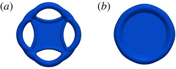
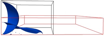
Head-on collisions of two identical droplets at high Weber numbers result in an extremely thin lamella, which artificially ruptures in numerical simulations even at relatively fine grid resolutions. The rupture of the thin lamella leads to a deviation of the shape of the collision complex as illustrated exemplarily in figure 1. Similar lamella ruptures are also noted in numerical works of Pan & Suga (Reference Pan and Suga2005), Nikolopoulos, Theodorakakos & Bergeles (Reference Nikolopoulos, Theodorakakos and Bergeles2009), Focke & Bothe (Reference Focke and Bothe2011) and Focke (Reference Focke2013). In experimental studies of binary droplet collisions, the lamella rupture is not observed even when the Weber number is increased to
 $We=2876$
(Roth et al.
Reference Roth, Rieber and Frohn1999), which confirms that the mentioned lamella rupture is artificial and must be prevented in numerical studies in order to capture sound physics.
Lamella rupture (a) versus stabilized lamella (b).

According to the work of Focke & Bothe (Reference Focke and Bothe2011) and Focke (Reference Focke2013) in particular, the interaction in computing the surface tension forces of both sides of the lamella leads to artificial lamella rupture. With respect to the CSS model in FS3D, the surface tension force is computed from the divergence of the surface stress tensor, which is computed from a smoothed phase indicator field
 $\tilde{f}$
. Both the smoothing of the phase indicator and the calculation of the divergence of the surface stress tensor are carried out in stencils of 27 cells (
 $3^{3}$
cells). Altogether the surface tension force in each cell containing a surface is affected by phase indicators in a stencils of 125 cells (
 $5^{3}$
cells) (Focke & Bothe Reference Focke and Bothe2011). When the lamella is resolved by fewer than four cells, the block of 125 cells contains interface cells from the opposite side of the lamella, which causes an unphysical interaction that leads to the lamella rupture.
In addition, the surface reconstruction is affected by the artificial interface interaction as well. The surface reconstruction is unambiguously determined by the
 $f$
-field and the surface normal, which is computed as
 $$\begin{eqnarray}\boldsymbol{n}=-\frac{\boldsymbol{{\rm\nabla}}f}{\Vert \boldsymbol{{\rm\nabla}}f\Vert },\end{eqnarray}$$
where
 $f$
is not smoothed in contrast to
 $\tilde{f}$
in (2.10) (Rieber Reference Rieber2004). The computation of the surface normal is conducted in a stencil of 27 cells. If this contains additional interface cells from the opposite side of the lamella, the computation of the surface normal is affected and, hence, the surface reconstruction as well.
Both the problem in computing the surface tension force and the problem with the surface reconstruction can be prevented by identifying the lamella region and then treating the cells of the opposite side of the lamella as ‘fully wetted’. Focke & Bothe (Reference Focke and Bothe2011) implemented the lamella stabilization method for head-on collisions of two identical droplets based on the collision of a droplet on a symmetry plane, which is equivalent to the head-on droplet collision. The boundary conditions of a symmetry plane are incorporated using two layers of dummy cells adjacent to the computational domain (Blazek Reference Blazek2001). Focke & Bothe (Reference Focke and Bothe2011) sort out the lamella region from the rim region of the collision complex by detecting the direct neighbouring cells of an interface cell (we denote it here as a ‘target’ cell) in the first layer of the computational grid on the symmetry plane. If not every direct neighbouring cell contains fluid, the target cell is defined as ‘rim’. Target cells whose neighbouring cells are all also interface cells are defined as ‘lamella’. The phase indicator is then set to
 $f=1$
in the dummy cells in the lamella region, thereby avoiding the above-mentioned unphysical interaction. It turns out that, in this way, the lamella is well stabilized. However, the rim region is not optimally identified since only the direct neighbouring cells of a target cell are detected, which may lead to confusion of the rim region with the lamella region.
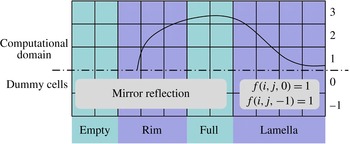
In order to correctly identify the rim region we introduce some modifications to the work of Focke & Bothe (Reference Focke and Bothe2011). The implementation of this modified lamella stabilization method is based on a collision complex on a symmetry plane as well. The procedure is as follows (see figure 2 for a schematic diagram):
-
(i) The region is denoted as ‘empty’ if the phase indicator in the first layer of computational cells of this region equals
 $0$
(
$f(i,j,1)=0$
). The region is denoted as ‘full’ if the phase indicators in both the first and second layers equal
$1$
(
$f(i,j,1)=1$
and
$f(i,j,2)=1$
).
-
(ii) The algorithm detects all the neighbouring cells of the remaining cells in the first layer as follows: if one of the phase indicators
$f(i+3,j,1)$
,
$f(i+3,j+3,1)$
,
$f(i,j+3,1)$
,
$f(i-3,j+3,1)$
,
$f(i-3,j,1)$
,
$f(i-3,j-3,1)$
,
$f(i,j-3,1)$
,
$f(i+3,j-3,1)$
equals
$0$
, the region is denoted as ‘rim’; the remaining region is set to ‘lamella’. -
(iii) The phase indicators of dummy cells in the lamella region are set to
$1$
and are mirrored in the remaining regions. -
(iv) The surface normal and the surface tension force are computed from this modified
$f$
-field. -
(v) The modification of the
$f$
-field in dummy cells is discarded.











Schematic diagram of lamella stabilization.

In addition, the lamella stabilization of Focke & Bothe (Reference Focke and Bothe2011) keeps the
 $f$
-value in the lamella from falling below
 $10^{-6}$
during the transport of the
 $f$
-field. Focke & Bothe (Reference Focke and Bothe2012) extended the work of Focke & Bothe (Reference Focke and Bothe2011) for simulating off-centre droplet collision without a symmetry plane by adding fluid into the lamella to stabilize it. In contrast, no mass needs to be added in the present work in order to keep the lamella from rupturing.
3.1. Validation
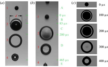
In order to validate the new implementation of the lamella stabilization, the numerical results are compared with the experimental work of Roth et al. (Reference Roth, Mercadé, Gomaa, Focke, Bothe, Roisman, Weigand and Gavaises2013). The fluid is isopropanol. Figure 3 shows that the shapes of the collision complex resulting from the simulation and from the experiment are in good agreement. The slight corrugation at the rim of the collision complex at the later stage of the deformation (around
 $400~{\rm\mu}\text{s}$
) is also predicted by the simulation. It should be mentioned here that all the visualizations in this paper related to the comparison with experiments are accomplished by using the open-source ray tracer program POV-Ray (http://www.povray.org) in order to facilitate a better comparison, since POV-Ray enables a clear visualization of the lamella of the collision complex.
Comparison of the predicted shapes of the collision complex (c) with the experimental results (a,b) of Roth et al. (Reference Roth, Mercadé, Gomaa, Focke, Bothe, Roisman, Weigand and Gavaises2013). The two columns of the collision complexes in the experiment result from double exposure. See Roth et al. (Reference Roth, Mercadé, Gomaa, Focke, Bothe, Roisman, Weigand and Gavaises2013) for more details about the experimental set-ups. The Weber number and Reynolds number are
 $We=268$
,
 $Re=426$
. The simulations are conducted with
 $288\times 288\times 96$
equidistant cubic cells using three symmetry planes.

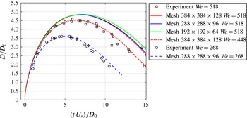
The developments of the diameter
 $D$
of the collision complex for two cases with different Weber numbers
 $We=268$
and
 $We=518$
are presented in figure 4. In the simulations,
 $D$
is defined as the average diameter on the collision plane and is computed based on the centre of the PLIC surfaces; in the experiment, the measurement of
 $D$
is indicated in the experimental part of figure 3 (denoted there as
 $d$
). The diameter of the collision complex and the time are presented in a dimensionless form defined by
 $D^{\ast }=D/D_{0}$
and
 $t^{\ast }=tU_{r}/D_{0}$
respectively. In the case of
 $We=268$
(the same case as presented in figure 3), the development of
 $D$
predicted by the simulation is in very good agreement with the experimental results. In the case of
 $We=518$
, the curves for the diameter of the collision complex converge with increasing grid resolution. However, the limit curve lies above the corresponding experimental results. We attribute this deviation to both the numerical and experimental inaccuracies. In the experiment, errors arise and are accumulated in measuring the droplets’ material and kinetic parameters. For example, assuming that the velocity in the experiment might be smaller than measured, we performed an additional simulation with a smaller Weber number (
 $We=448$
, the relative velocity is 7 % smaller than the original), which achieves a very good accordance. In total, these comparisons show the ability of the lamella stabilization method in predicting the development of the collision complex.
Comparison of the predicted diameters of the collision complex with experimental results. The case
 $We=268$
is the same case as presented in figure 3. The Reynolds number of the case
 $We=518$
is
 $Re=600$
. The Reynolds number of the case
 $We=448$
is
 $Re=558$
. The simulations are conducted with equidistant cubic cells using three symmetry planes.

4. Domain adjustment
Based on the assumption that the gas phase (air) in the computational domain does not affect the collision dynamics significantly, we employ a domain adjustment to reduce the computational effort. This technique is based on the work of Focke (Reference Focke2013). The procedure to implement this technique is described below (see the schematic diagram in figure 5):
-
(i) The computation is started in a cuboid computational domain.
-
(ii) The computation is stopped before the collision complex reaches the boundary of the computational domain. The computational data are saved in restart-files for each CPU.
-
(iii) The computational domain is reinitialized by enlarging the domain in the direction in which the collision complex is extending, and shrinking the domain in the direction in which the collision complex is receding.
-
(iv) Only the computational data in the overlap region of the old and new computational domains are loaded. The velocities in the non-overlapping domain are set to zero. The relative grid resolution is kept unchanged. Then the computation is restarted without additional modification. Solving the pressure Poisson equation and conducting velocity correction as in a normal time step without domain adjustment ensure a divergence-free velocity field after the domain change.
Using this technique either the number of necessary CPUs can be reduced or the computational resolution can be enlarged. The surface energy at the time
 $t^{\ast }=10$
normalized with initial surface energy obtained with and without this domain adjustment technique for the aforementioned case
 $We=518$
computed with
 $384\times 384\times 128$
cells is
 $6.463$
and
 $6.469$
, respectively. The deviation is very small, which reveals that the domain adjustment technique is usable in the simulation of binary droplet collisions at high Weber numbers.
Domain adjustment.

5. Numerical set-ups
In this study we consider only head-on collisions of two identical droplets. The material properties of the air/water system are:
 ${\it\eta}_{L}=1.000\times 10^{-3}~\text{N}~\text{s}~\text{m}^{-2}$
,
 ${\it\rho}_{L}=1000~\text{kg}~\text{m}^{-3}$
,
 ${\it\eta}_{G}=1.8\times 10^{-5}~\text{N}~\text{s}~\text{m}^{-2}$
,
 ${\it\rho}_{G}=1.2~\text{kg}~\text{m}^{-3}$
and
 ${\it\sigma}=72.0\times 10^{-3}~\text{N}~\text{m}^{-1}$
. In all simulations at least one symmetry plane, namely the collision plane, is used since the implementation of the lamella stabilization is based on this symmetry plane as described in § 3. In the case of
 $We=1520$
, owing to the extremely high collision energy, we utilize two additional symmetry planes to increase the computational resolution with a restricted number of CPUs. The cuboid domain is decomposed into equidistant cubic cells. The slip conditions are prescribed on the symmetry planes; the homogeneous Neumann boundary condition for the velocity and zero pressure are prescribed on all the other boundary planes. The simulations are started at
 $t^{\ast }=0$
when the distance between the centres of the spherical initial droplets is
 $D_{0}$
. The parameters of the cases that are discussed in the following sections with corresponding set-ups are summarized in table 1.
Set-ups of conducted simulations.

The time step is restricted dynamically by the Courant–Friedrichs–Lewy (CFL) condition. The maximum allowed Courant number is set to
 $0.05$
, which means
 $$\begin{eqnarray}{\rm\Delta}t\leqslant \frac{0.05{\rm\Delta}x}{|\boldsymbol{u}_{max}|}.\end{eqnarray}$$
We select a very small Courant number to ensure a high temporal resolution, which avoids oscillation in the velocity field observed at larger Courant numbers. The stability conditions related to the capillary wave and the fluid viscosity are also fulfilled at this small time step.
In all our simulations of droplet collisions we observe that a small quantity of air is enclosed in the collision complex. Simulating collision between droplets of high and low viscosity, Focke et al. (Reference Focke, Kuschel, Sommerfeld and Bothe2013) also observed the entrainment of air and argued that the entrainment is attributed to the failure of the interface reconstruction when the approaching interfaces of the colliding droplets appear in one cell. We conducted a test simulation replacing the entrainment of air with water. The evolution of the collision complex does not show any significant deviation compared to the corresponding results with entrainment of air. Hence, the decision was made to keep the entrainment of air untouched.
5.1. Role of imposed disturbances
In order to obtain physically reasonable numerical results in simulating splashing phenomena at droplet impact on a fluid film, Rieber & Frohn (Reference Rieber and Frohn1999) imposed an artificial disturbance to the initial velocity field of the droplet and fluid film with a Gaussian distribution. The standard deviation of the Gaussian distribution is selected up to half of the initial velocity of the droplets. Analogously, we add random noise to the initial velocity field:
 $$\begin{eqnarray}\boldsymbol{u}=\boldsymbol{u}_{0}+\tilde{\boldsymbol{u}},\end{eqnarray}$$
where
 $\tilde{\boldsymbol{u}}$
is the added velocity which is distributed over the whole computational domain according to the Gaussian distribution. The standard deviation of the Gaussian distribution for each component of
 $\tilde{\boldsymbol{u}}$
is denoted as
 ${\rm\Delta}U$
, which is normalized with the relative velocity of the colliding droplets
 $U_{r}$
. Based on the case of
 $We=442.3$
, we first examine the influence of the disturbance strength and the time when the disturbance is exerted. The shapes of the collision complex at
 $t^{\ast }=12.72$
with different
 ${\rm\Delta}U$
imposed at
 $t^{\ast }=0$
are presented in figure 6. As expected, the deformation of the collision complex becomes more violent when
 ${\rm\Delta}U$
is increased. The shapes of the collision complex at
 $t^{\ast }=12.72$
with
 ${\rm\Delta}U=1\,\%$
imposed at different times are presented in figure 7. One observes that the deformation of the collision complex which is disturbed very early after collision (
 $t^{\ast }=0.1$
) is most violent. If the disturbance is exerted after
 $t^{\ast }=0.1$
, its influence tends to vanish with increasing disturbance time, again as to be expected.
Collision complex at
 $t^{\ast }=12.72$
resulting from a disturbance imposed at
 $t^{\ast }=0$
with different
 ${\rm\Delta}U$
. (a) No disturbance, (b)
 ${\rm\Delta}U=0.2\,\%$
, (c)
 ${\rm\Delta}U=0.5\,\%$
, (d)
 ${\rm\Delta}U=1\,\%$
, (e)
 ${\rm\Delta}U=2\,\%$
.

Collision complex at
 $t^{\ast }=12.72$
resulting from a disturbance imposed at different times
 $t_{dist}^{\ast }$
with
 ${\rm\Delta}U=1\,\%$
. (a) No disturbance, (b)
 $t_{dist}^{\ast }=0$
, (c)
 $t_{dist}^{\ast }=0.1$
, (d)
 $t_{dist}^{\ast }=0.2$
, (e)
 $t_{dist}^{\ast }=0.5$
.

All the simulations presented in the following sections are conducted both with and without disturbances to further investigate the influence of the disturbance on the collision dynamics. The disturbances are exerted at
 $t^{\ast }=0$
, which corresponds to the reality that at the beginning of the collision there is an initial disturbance of the colliding droplets and a disturbance of the surroundings. We select the disturbance strength
 ${\rm\Delta}U=1\,\%$
for the three cases to be studied.
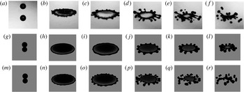
Photographs and visualized simulation results of the head-on collision of water droplets with
 $We=442.3$
,
 $Re=6207.3$
. (a–f) Experimental result of Pan et al. (Reference Pan, Chou and Tseng2009). (g–l) Simulation results without initial disturbance. (m–r) Simulation result with an initial disturbance of
 ${\rm\Delta}U=1\,\%$
.
 $t^{\ast }=-1.15$
(a), 3.81 (b), 6.28 (c), 10.42 (d), 12.07 (e), 13.72 (f), 0 (g,m), 3.82 (h,n), 6.23 (i,o) 10.43 (j,p), 12.08 (k,q), 13.74 (l,r).

6. Results and discussions
6.1. Comparison with experiments
We compare our numerical results with the experimental work of Pan et al. (Reference Pan, Chou and Tseng2009). The comparison of the evolution of the droplet complexes for the case of a relatively low Weber number (
 $We=442.3$
) is presented in figure 8. The deformation history of the droplet complex that results from simulation without an initial disturbance (g–l) can be described as follows: a fluid sheet is formed in the middle of the collision complex after the coalescence of the droplets (not shown in the images). This fluid sheet is radially extended within the collision plane and forms a toroidal rim at the edge. At about the maximum diameter of the collision complex (
 $t^{\ast }=6.23$
; the wave shown in the lamella region results from the breakup of air entrainment), an obvious corrugation of the rim is observed. The corrugation is then magnified and evolves into finger-like structures, which grow at the receding stage of the deformation. Compared to the experimental results, the appearance of the corrugation and the evolution of the fingers are delayed so that no secondary droplets are detached from the rim of the collision complex. The evolution of the collision complex that results from the simulation with an initial disturbance is quite synchronized with the experimental results and yields detachment of secondary droplets, which corresponds well with the experimental results. The development of fingers in the simulation with an initial disturbance is not regular because of the stochastic nature of the Gaussian distribution of the initial disturbance.
Figure 9 presents the results for a higher Weber number (
 $We=805.2$
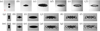
). In this case the detachment of secondary droplets starts before the maximum diameter is reached in the simulations both with and without an initial white noise. However, even in the simulation without an initial disturbance, the secondary droplets are detached earlier than in the experimental results. The reason for this deviation will be explained in the following section. In the visualizations of the numerical part in figure 9, some secondary droplets at the periphery of the domain are much brighter, since these droplets flying out of the computational domain cannot be correctly captured by POV-Ray.
Photographs and visualized simulation results of the head-on collision of water droplets with
 $We=805.2$
,
 $Re=6370.0$
. (a–f) Experimental result of Pan et al. (Reference Pan, Chou and Tseng2009). (g–l) Simulation results without initial disturbance. (m–r) Simulation result with an initial disturbance of
 ${\rm\Delta}U=1\,\%$
.
 $t^{\ast }=-0.36$
(a), 0.95 (b), 3.58 (c), 12.77 (d), 14.08 (e), 15.40 (f), 0 (g,m), 0.88 (h,n), 3.51 (i,o), 12.87 (j,p) 14.04 (k,q) 15.50 (l,r).

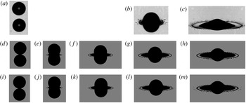
Figure 10 presents the results for a much higher Weber number (
 $We=1520$
). The detachment of secondary droplets from the rim at the very early stage of the deformation called ‘prompt splashing’ is reproduced in the simulation with an initial disturbance (i–m), which corresponds well with the experimental results. The results without an initial disturbance (d–h) yield no secondary droplets until
 $t^{\ast }=1.05$
. Due to the restriction of the computational resource, the simulation is only conducted until
 $t^{\ast }=1.05$
. Kuan et al. (Reference Kuan, Pan and Shyy2014) concluded on the basis of their numerical observations that at this extremely high Weber number the whole toroidal rim will be separated from the sheet and will then break up into secondary droplets. In contrast, our results show that the rim is still connected to the sheet and the secondary droplets are splattered out from the rim. We presume that Kuan et al. (Reference Kuan, Pan and Shyy2014) reached their conclusion because the lamella was not stabilized, which typically leads to a non-physical lamella rupture at the joint between the lamella and the sheet and therefore the separation of the rim from the sheet.
Photographs and visualized simulation results of the head-on collision of water droplets with
 $We=1520$
,
 $Re=8750.0$
. (a–c) Experimental result of Pan et al. (Reference Pan, Chou and Tseng2009). (d–h) Simulation results without initial disturbance. (i–m) Simulation result with an initial disturbance of
 ${\rm\Delta}U=1\,\%$
.
 $t^{\ast }=-0.22$
(a), 0.73 (b), 2.49 (c), 0 (d,i), 0.23 (e, j), 0.46 (f,k), 0.73 (g,l), 1.05 (h,m).

6.2. Quantification of the rim development
We conduct a comprehensive quantification of the rim development for the case
 $We=442.3$
, which is in best agreement with the experiment. In the following, for simplification, the length is rescaled by the initial droplet radius and the velocity by the initial velocity of one droplet. The
 $^{\ast }$
that represents dimensionless time is dropped. We extract the radius of the collision complex on the collision plane based on isosurfaces of
 $f=0.5$
and compute the amplitude
 $a_{m}$
of instability mode
 $m$
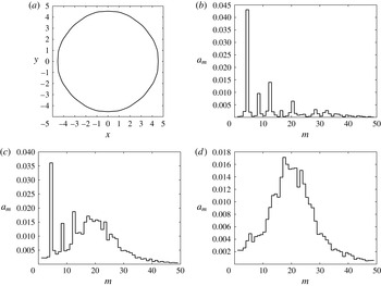
by conducting fast Fourier transformation (FFT). The amplitudes and the corresponding curve of the frontier of the collision complex for the case
 $We=442.3$
without imposed noise at
 $t=3.82$
are shown in figure 11(a,b). One observes that
 $m=4$
dominates the rim instability, which corresponds to the anisotropic Cartesian grid arrangement. Furthermore, all the other strong peaks correspond to the harmonics of the mode
 $m=4$
. The amplitudes of modes
 $m=4n$
, on one hand, occur in form of the rim instability. On the other hand, they occur systematically due to the grid structure and, hence, cannot be suppressed. This explains why in the case
 $We=805.2$
without imposed disturbance, the rim instability is already stronger than in the corresponding experiment.
(a) Extracted curve of the frontier of the collision complex on the collision plane for the case
 $We=442.3$
without imposed noise at
 $t=3.82$
. (b) Corresponding amplitudes. (c) Averaged amplitudes of
 $10$
repeated simulations with imposed disturbance of the same strength (
 ${\rm\Delta}U=1\,\%$
) also at
 $t=3.82$
. (d) The amplitudes of modes
 $m=4n$
in (c) are replaced with interpolated values of the neighbouring modes.

To include the randomness of the disturbance, we repeat the same simulation
 $10$
times with different disturbance of same strength (
 ${\rm\Delta}U=1\,\%$
). We then average the spectrum diagram for the radius of the collision complex. To minimize the unwanted effect of the grid anisotropy and its harmonics (exemplarily shown in figure 11
c), we replace the amplitudes of modes
 $m=4n$
by interpolated amplitude values of the neighbouring modes (exemplarily shown in figure 11
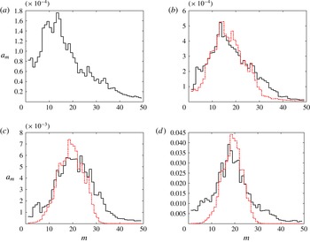
d). The averaged spectrum diagrams for a large time span are shown in figure 12. We observe that, during the time evolution, the region of the largest amplitudes is first shifted to larger modes and then moves slightly backwards.
Averaged amplitudes of 10 numerical experiments (black solid line) and amplitudes predicted by PR theory (red dashed line).
 $t=0.25$
(a), 0.64 (b), 2.54 (c), 5.09 (d).

The mean rim radius
 $r_{0}$
is computed based on the case
 $We=442.3$
without an initial disturbance and serves as the average value for the corresponding
 $10$
repeated simulations. The rim radius
 $r_{0}$
is computed implicitly, based on the volume equivalence
 $$\begin{eqnarray}V_{\mathit{rim}}=2{\rm\pi}R_{c}{\rm\pi}r_{0}^{2},\end{eqnarray}$$
where
 $V_{\mathit{rim}}=V_{\mathit{cell}}\int _{\mathit{rim}}f(x,y,z)\,\text{d}x\,\text{d}y\,\text{d}z$
. The rim region, over which the integration is computed, is determined from the location of the minimum interface height normal to the collision plane, which always appears adjacent to the rim and separates the rim from the lamella. In (6.1),
 $R_{c}=R_{0}-r_{0}$
is the radius of the rim centreline and
 $R_{0}$
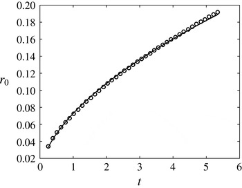
is the amplitude of the zeroth mode of the FFT analysis. The rim radius is plotted in figure 13. We found that the evolution of the radius can be fitted best by a power law according to
 $$\begin{eqnarray}r_{0}=0.569\,t^{\,0.073}.\end{eqnarray}$$
Evolution of the rim radius and its best fitting curve.

The radius of the collision complex on the collision plane
 $R(t)$
, the rim velocity
 ${\dot{R}}(t)$
and rim acceleration
 $\ddot{R}(t)$
are also computed for the case
 $We=442.3$
without an initial disturbance:
 $R(t)$
is computed as the average value of PLIC-surface centre positions;
 ${\dot{R}}(t)$
and
 $\ddot{R}(t)$
are then derived from
 $R(t)$
by forward differencing. While computing the time difference,
 $R(t)$
and
 ${\dot{R}}(t)$
are locally smoothed by least-squares fitting to eliminate high-frequency oscillations. The evolution of
 $R(t)$
,
 ${\dot{R}}(t)$
and
 $\ddot{R}(t)$
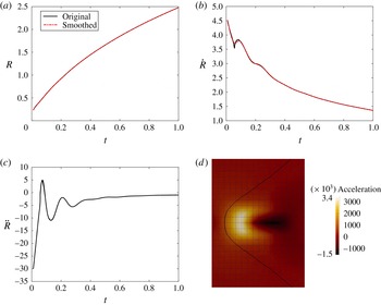
and the corresponding smoothed lines are shown in figure 14. The curves start at
 $t=0.01$
to avoid the singularity at
 $t=0$
. Surprisingly, we observe an oscillation in the development of the rim acceleration, and the acceleration is even positive for quite a long period, which is in contradiction to the common opinion that the rim only decelerates (Kim et al.
Reference Kim, Feng and Chun2000). The acceleration field computed by means of DNS, shown exemplarily in figure 14(d) for
 $t=0.07$
, confirms that the frontier of the collision complex on the collision plane is located in the region of positive acceleration. According to Kim et al. (Reference Kim, Feng and Chun2000), the rim is decelerated as a result of its radial expansion. In the specific case of binary droplet collisions at early time, the surface force pulls the interface outwards due to the negative surface curvature on the collision plane (see figure 14
d) after the droplets coalesce and before the fluid sheet is ejected on the collision plane. This additional acceleration contributes to the positive acceleration. After the toroidal rim is formed, it oscillates essentially like an oscillating fluid cylinder. According to Rayleigh (Reference Rayleigh1879), the angular frequency of a fluid cylinder for mode
 $m$
can be estimated as
 $$\begin{eqnarray}{\it\omega}_{m}=\sqrt{(m^{3}-m)\frac{{\it\sigma}}{{\it\rho}r_{0}^{3}}}.\end{eqnarray}$$
From figure 14(c), the oscillation period is extracted as the time difference between the first two minima, resulting in a value of
 $0.147$
. Applying (6.3), the corresponding calculated oscillation period for mode
 $m=2$
is
 $0.145$
. This very good agreement of the oscillation period confirms that the rim oscillates and that this oscillation is governed by (6.3).
(a) Evolution of the radius of the collision complex. (b) Evolution of the rim velocity. (c) Evolution of the rim acceleration. (d) Acceleration field by means of DNS at
 $t=0.07$
.

As mentioned in the introduction, the reason for the rim instabilities is so far still under debate. The RT instability and the PR instability theories are the most popular candidates that are used to explain the rim instability. In the following sections, we examine the two mentioned instability patterns based on the quantifications obtained for the case
 $We=442.3$
.
6.3. RT instability
In the classic RT theory (Taylor Reference Taylor1950), a decelerating flat interface that moves in the direction from a dense fluid to a less dense fluid is unstable. Kim et al. (Reference Kim, Feng and Chun2000) extended the RT theory for studying the rim instability of a droplet spreading on a solid substrate to cylindrical coordinates. In fact, their model is more suitable for studying the rim instability in binary droplet collisions where the effect of contact angle, which is not included in their model, is not present. The derivation of the model of Kim et al. (Reference Kim, Feng and Chun2000) starts with the spectral decomposition of the radius of the collision complex according to
 $$\begin{eqnarray}\bar{R}({\it\phi},t)=R_{0}(t)+\mathop{\sum }_{m=1}^{N}a_{m}\cos \,m{\it\phi},\end{eqnarray}$$
where
 ${\it\phi}$
is the angle and
 $a_{m}$
the amplitude of mode
 $m$
. Below, we employ
 $R(t)$
given in figure 14 instead of
 $R_{0}(t)$
since the latter is only computed for certain times by FFT analysis in postprocessing. It is not at our disposal for all time steps. The difference between
 $R(t)$
and
 $R_{0}(t)$
is small.
The derivation ends with solving a second-order linear differential equation for the amplitude of mode
 $m$
(Kim et al.
Reference Kim, Feng and Chun2000):
 $$\begin{eqnarray}\ddot{a}_{m}+{\it\alpha}(t){\dot{a}}_{m}+{\it\beta}(t)a_{m}=0,\end{eqnarray}$$
where
 ${\it\alpha}$
and
 ${\it\beta}$
are given as
 $$\begin{eqnarray}{\it\alpha}(t)=2\frac{{\dot{R}}}{R},\end{eqnarray}$$
 $$\begin{eqnarray}{\it\beta}(t)=\frac{(m+1)}{R^{3}}\left(\frac{m(m-1)}{We}+R^{2}\ddot{R}\right).\end{eqnarray}$$
Here
 $We$
is
 $1/8$
of the Weber number that is defined for binary droplet collisions. Equation (6.5) is solved numerically by means of a first-order explicit Euler scheme.
We plug
 $R(t)$
,
 ${\dot{R}}(t)$
and
 $\ddot{R}(t)$
into (6.6) and (6.7) and evaluate the perturbation growth from
 $t=0.13$
to
 $t=0.25$
, using amplitudes at
 $t=0.13$
computed by FFT analysis to serve as initial values
 $a(0)$
. The other initial value
 ${\dot{a}}(0)$
is set to
 $0$
. We did not start at an earlier time for two reasons: (1) the FFT analysis at an earlier time was not reliable due to the restriction on grid resolution for small
 $R$
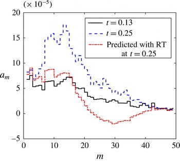
; (2) the acceleration at early time is positive over a large time span, which according to RT theory (Taylor Reference Taylor1950) decreases the rim stability. The diagrams in figure 15 show that the amplitudes with small modes are magnified by the rim deceleration, which is in agreement with the FFT analysis. However, the amplitude growth computed by Rayleigh–Taylor theory is rather small compared to the amplitude growth obtained from FFT analysis of our numerical results. Similar statements are also given by Agbaglah & Deegan (Reference Agbaglah and Deegan2014).
The evolution of amplitude from
 $t=0.13$
to
 $t=0.25$
obtained from FFT analysis and the prediction with RT theory.

6.4. PR instability
The formation of the toroidal rim finishes at around
 $t=0.25$
, allowing us to examine the PR theory after
 $t=0.25$
. We use the same PR expression derived by Zhang et al. (Reference Zhang, Brunet, Eggers and Deegan2010) for predicting the amplitude evolution of mode
 $m$
. We briefly describe the mathematical model below; further details are given by Zhang et al. (Reference Zhang, Brunet, Eggers and Deegan2010).
The spectral decomposition of the local rim radius is written as
 $$\begin{eqnarray}r({\it\phi},t)=r_{0}(t)+{\it\epsilon}({\it\phi},t)=r_{0}(t)+\mathop{\sum }_{m=1}^{N}a_{m}\cos \,m{\it\phi},\end{eqnarray}$$
where
 ${\it\epsilon}$
is the small perturbation of
 $r_{0}$
. The growth rate
 $S_{m}$
of the
 $m\text{th}$
mode is implicitly computed on a cylinder of constant radius via
 $$\begin{eqnarray}2x^{2}(x^{2}+y^{2})\frac{\text{I}_{1}^{\prime }(x)}{\text{I}_{0}(x)}\left(1-\frac{2xy}{x^{2}+y^{2}}\frac{\text{I}_{1}(x)}{\text{I}_{1}(y)}\frac{\text{I}_{1}^{\prime }(y)}{\text{I}_{1}^{\prime }(x)}\right)-x^{4}+y^{4}=\frac{{\it\rho}{\it\sigma}r_{0}}{{\it\eta}^{2}}\frac{x\text{I}_{1}(x)}{\text{I}_{0}(x)}(1-x^{2}),\end{eqnarray}$$
where
 $x=k_{m}r_{0}$
,
 $k_{m}=m/R_{c}$
is the wavenumber of the
 $m\text{th}$
mode,
 $y^{2}=x^{2}+{\it\rho}S_{m}r_{0}^{2}/{\it\eta}$
, and
 $\text{I}_{n}$
are modified Bessel functions of the first kind. Including the growth and the expansion of the rim, the time evolution of the perturbation is given by
 $$\begin{eqnarray}\frac{\text{d}\,\text{ln}\,{\it\epsilon}(t)}{\text{d}t}=-\frac{s}{2}+S_{m},\end{eqnarray}$$
where
 $s$
is the stretch rate due to the expansion of the rim given by
 $s=\dot{R_{c}}/R_{c}$
. Equation (6.10) can then be integrated over time to obtain
 $$\begin{eqnarray}\text{ln}\frac{{\it\epsilon}(t)}{{\it\epsilon}(0)}=-\frac{1}{2}\text{ln}\frac{R_{c}(t)}{R_{c}(0)}+\int _{0}^{t}S_{m}\,\text{d}t^{\prime }.\end{eqnarray}$$
Using initial perturbation
 $a_{m}(0)$
, the amplitude of the
 $m\text{th}$
mode at
 $t$
is given as
 $$\begin{eqnarray}a_{m}(t)=a_{m}(0)\sqrt{\frac{R_{c}(0)}{R_{c}(t)}}\text{exp}\left(\int _{0}^{t}S_{m}(m/R_{c}(t),r_{0}(t))\,\text{d}t^{\prime }\right).\end{eqnarray}$$
We apply the amplitudes at
 $t=0.25$
(shown in figure 12
a) as initial conditions in (6.12) and compute the amplitude evolution, which is compared with FFT analysis of our numerical results in figure 12. Both the region of maximum amplitudes and the amplitude scale in this region are predicted very well over quite a long time span, which strongly indicates that the evolution of the rim instability is dominated by the PR instability pattern after the toroidal rim is formed. The variation of the region of maximum amplitudes is simply due to both the different initial amplitudes of mode
 $m$
and their different amplification histories.
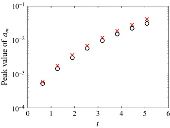
The theoretical peak amplitude value and the peak amplitude value obtained in the simulation are computed by fitting the corresponding spectrum diagram to a Gaussian distribution and compared in figure 16. It turns out that the peak amplitude is somewhat higher in the theoretical prediction. The overestimation factor computed on the basis of data shown in figure 16 is
 $1.23\pm 0.06$
. According to previous works, this deviation can be attributed to the presence of the fluid sheet that is attached to the rim but is neglected in the application of RP theory. Modelling the instability growth on a fluid cylinder combined with a planar sheet, Agbaglah, Josserand & Zaleski (Reference Agbaglah, Josserand and Zaleski2013), Roisman, Horvat & Tropea (Reference Roisman, Horvat and Tropea2006) and Roisman (Reference Roisman2010) showed that the presence of the fluid sheet stabilizes the rim instability. Zhang et al. (Reference Zhang, Brunet, Eggers and Deegan2010) stated that the transition from rim to sheet also slows the growth of the rim instability. Further study is required to verify the influence of the fluid sheet on the rim instability.
Theoretical maximum amplitude (red crosses) and the maximum amplitude in the simulation (black circles) versus time.

7. Conclusion
We simulated head-on collisions of binary water droplets at high Weber numbers by means of the modified lamella stabilization method. The comparison between numerical and experimental results reveals that the initial random disturbances have to be taken into account while comparing shapes of collision complexes obtained from simulation and experiment, since the development of the unstable rim is quite sensitive to the disturbances in the early stage of a collision. From the numerical side, the anisotropic grid arrangement is an unavoidable source of disturbance that may lead to the development of a stronger instability than in the experiment.
Based on our simulation results, the breakup mechanism of the rim at an extremely high Weber number (
 $We=1520$
) is not as different as at relatively lower Weber numbers in terms of whether the rim is completely detached from the fluid sheet before the formation of secondary droplets, which is in disagreement with the conclusion of Kuan et al. (Reference Kuan, Pan and Shyy2014).
At lower Weber number, our results confirm the dominance of a PR instability pattern in the development of rim instability, which is also concluded by Zhang et al. (Reference Zhang, Brunet, Eggers and Deegan2010) and Rieber & Frohn (Reference Rieber and Frohn1999). Furthermore, our results show that the amplitude magnification can also be well predicted by the PR-based theory over a long time span. In the early period of the collision, when the toroidal rim is not yet formed, we identified positive rim acceleration and rim oscillation for the first time. Our results confirm that the rim deceleration provides a small boost to amplitude growth in the region of small modes, as was stated in Agbaglah & Deegan (Reference Agbaglah and Deegan2014).
Acknowledgement
The authors gratefully acknowledge financial support provided by the German Research Foundation (DFG) within the scope of SFB-TRR 75.