2.1. PDF methods

The starting point is the definition of the temperature PDF as an ensemble average,

(2.1) $$\begin{eqnarray}f(T,\boldsymbol{x},t)=\langle {\it\delta}(T(\boldsymbol{x},t)-T)\rangle ,\end{eqnarray}$$

where the PDF $f(T,\boldsymbol{x},t)$ describes the probability of finding fluid of temperature $T$ at position $\boldsymbol{x}$ and time $t$ . Accordingly, $T$ is the sample space variable, while $T(\boldsymbol{x},t)$ is a realisation of the temperature field. The averaging process $\langle \cdot \rangle$ can be considered as an ensemble average; later, ensemble averages are evaluated from the numerics by a suitable volume and time average.

Since the definition in (2.1) includes an actual realisation $T(\boldsymbol{x},t)$ of the temperature field, it is now possible to calculate spatial and temporal derivatives of the PDF, i.e.  $\boldsymbol{{\rm\nabla}}f(T,\boldsymbol{x},t)$ and $(\partial /\partial t)f(T,\boldsymbol{x},t)$ . These derivatives contain unclosed terms in the form of conditional averages $\langle \cdot \mid T,\boldsymbol{x},t\rangle$ , where, e.g. the appearing conditionally averaged velocity $\langle \boldsymbol{u}\mid T,\boldsymbol{x},t\rangle$ is a function of the sample space variables $T$ , $\boldsymbol{x}$ and $t$ which defines the mean velocity for fluid of a given temperature, position and time.

Putting the aforementioned derivatives together and rearranging gives the desired evolution equation that describes the temperature PDF:

(2.2a ) $$\begin{eqnarray}\displaystyle \frac{\partial }{\partial t}f+\boldsymbol{{\rm\nabla}}\boldsymbol{\cdot }(\langle \boldsymbol{u}\mid T,\boldsymbol{x},t\rangle f) & = & \displaystyle -\frac{\partial }{\partial T}\left(\left\langle \frac{\partial }{\partial t}T+\boldsymbol{u}\boldsymbol{\cdot }\boldsymbol{{\rm\nabla}}T|T,\boldsymbol{x},t\right\rangle f\right)\end{eqnarray}$$

(2.2b ) $$\begin{eqnarray}\displaystyle & = & \displaystyle -\frac{\partial }{\partial T}(\langle {\rm\Delta}T\mid T,\boldsymbol{x},t\rangle f).\end{eqnarray}$$

$f(T,\boldsymbol{x},t)$

$T(\boldsymbol{x},t)$

We have thus obtained an evolution equation that links the shape of the temperature PDF to the conditionally averaged velocity $\langle \boldsymbol{u}\mid T,\boldsymbol{x},t\rangle$ and heat diffusion $\langle {\rm\Delta}T\mid T,\boldsymbol{x},t\rangle$ , which have to be supplied externally; in our case they are estimated from simulations.

2.2. Method of characteristics

The above evolution (2.2) that determines the temperature PDF is a first-order partial differential equation. That means that we can apply the method of characteristics (Courant & Hilbert Reference Courant and Hilbert1962; Sarra Reference Sarra2003) which lets us identify the average behaviour of fluid as it travels through phase space.

By applying the method of characteristics to the evolution equation, one can identify trajectories (the so-called characteristic curves or just characteristics) in phase space, along which the partial differential equation for the temperature PDF transforms into a set of ordinary differential equations for $T$ and $\boldsymbol{x}$ . The phase space is spanned by the variables that the temperature PDF depends upon, i.e.  $T$ , $\boldsymbol{x}$ and $t$ . The characteristics are defined by the conditional averages,

(2.3) $$\begin{eqnarray}\left(\begin{array}{@{}c@{}}{\dot{T}}\\ \dot{\boldsymbol{x}}\\ {\dot{t}}\end{array}\right)=\left(\begin{array}{@{}c@{}}\langle {\rm\Delta}T\mid T,\boldsymbol{x},t\rangle \\ \langle \boldsymbol{u}\mid T,\boldsymbol{x},t\rangle \\ 1\end{array}\right).\end{eqnarray}$$

This states that the characteristics are solutions $(T,\boldsymbol{x},t)^{\text{T}}$ of (2.3) that follow the vector field on the right-hand side of the above equation; the vector field is regarded as the phase space velocity. From the last line of (2.3), ${\dot{t}}=1$ , it becomes clear that the parametrisation of the characteristics in phase space, i.e. the arc length, is the same as the time of the system – a fast movement in phase space therefore has to be seen in the temporal sense.

It is important to note that, since the characteristics are governed by the conditionally averaged vector field, they show the average behaviour of a fluid parcel in phase space. In other words, the characteristics can be seen as the mean evolution of an ensemble of Lagrangian particles that share the same coordinates in phase space. This is what Pope (Reference Pope1985, § 4.5) refers to as conditional particles – quasi-particles following the conditionally averaged vector field (2.3) that show the mean Lagrangian evolution and that have the same statistics as Lagrangian particles. By examining the conditionally averaged vector field and the resulting characteristic curves, one can investigate the mean transport properties of the fluid through phase space and gain insight into the mean heat transport properties of Rayleigh–Bénard convection. Since the characteristics are trajectories in phase space, the framework can be seen as a quasi-Lagrangian description, but it must be stressed that it is achieved by utilising the statistics of the Eulerian fields alone.

Along the characteristics, the partial differential equation (2.2) becomes an ordinary differential equation which can be integrated. Thus, the temperature PDF along a certain characteristic evolves according to

(2.4) $$\begin{eqnarray}\displaystyle f(T(t),\boldsymbol{x}(t),t) & = & \displaystyle f(T(t_{0}),\boldsymbol{x}(t_{0}),t_{0})\nonumber\\ \displaystyle & & \displaystyle \times \,\text{exp}\left[-\int _{t_{0}}^{t}\!\text{d}t^{\prime }\,\left(\boldsymbol{{\rm\nabla}}\boldsymbol{\cdot }\langle \boldsymbol{u}\mid T,\boldsymbol{x},t\rangle +\frac{\partial }{\partial T}\langle {\rm\Delta}T\mid T,\boldsymbol{x},t\rangle \right)_{T(t^{\prime }),\boldsymbol{x}(t^{\prime }),t^{\prime }}\right].\nonumber\\ \displaystyle & & \displaystyle\end{eqnarray}$$

Here, the integral is a line integral along a characteristic from $t_{0}$ to $t$ . The integral kernel is the phase space divergence $\boldsymbol{{\rm\nabla}}\boldsymbol{\cdot }\langle \boldsymbol{u}\mid T,\boldsymbol{x},t\rangle +(\partial /\partial T)\langle {\rm\Delta}T\mid T,\boldsymbol{x},t\rangle$ evaluated at the phase space position given by the characteristic for time $t^{\prime }$ , i.e.  $(T(t^{\prime }),\boldsymbol{x}(t^{\prime }),t^{\prime })^{\text{T}}$ . This equation tells us that the temperature PDF along the characteristic that connects the initial point $(T(t_{0}),\boldsymbol{x}(t_{0}),t_{0})^{\text{T}}$ with the point $(T(t),\boldsymbol{x}(t),t)^{\text{T}}$ in phase space changes according to the integrated phase space divergence. As an alternative interpretation, (2.4) determines how the temperature PDF for $t$ is traced back to the PDF for $t_{0}$ . While we will not further investigate (2.4) in the numerical results of the next section, we include it for completeness.

So far we have kept the description as general as possible, but usually, a Rayleigh–Bénard set-up has a number of statistical symmetries which simplify the problem, i.e. the phase space dimension is reduced and the estimation of the unknown conditional averages from numerical simulation is simplified. In the next section, we will apply the framework that has been outlined to three different Rayleigh–Bénard geometries with different symmetries and discuss the findings.

3.1. Three-dimensional convection with periodic horizontal boundaries

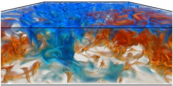
First, we consider three-dimensional convection with periodic horizontal boundaries in the statistically stationary state. A snapshot of the instantaneous temperature field taken from the numerics can be seen in figure 1. The parameters of the simulation are $\mathit{Ra}=2.4\times 10^{7}$ , $\mathit{Pr}=1$ and the aspect ratio of the periodic box is ${\it\Gamma}=4$ . The two horizontal plates have a constant temperature and a no-slip velocity boundary condition. The numerical set-up is a tri-periodic pseudospectral direct numerical simulation, where the boundary conditions are enforced by volume penalization methods (Angot, Bruneau & Fabrie Reference Angot, Bruneau and Fabrie1999; Schneider Reference Schneider2005; Keetels et al. Reference Keetels, D’Ortona, Kramer, Clercx, Schneider and van Heijst2007; Lülff et al. Reference Lülff, Wilczek and Friedrich2011). The equidistant resolution in the $x$ , $y$ and $z$ directions are $512\times 512\times 128$ grid points, and in the vertical direction $5$ grid points fall into the boundary layers, according to the criteria given by Shishkina et al. (Reference Shishkina, Stevens, Grossmann and Lohse2010). We calculated the statistical quantities from an ensemble consisting of $571$ snapshots, and the snapshots were taken $3.75$ free-fall time units apart.

Figure 1.

Snapshot of the temperature field in three-dimensional Rayleigh–Bénard convection. Hot fluid rising up from the bottom plate is reddish, while cold fluid falling down from the top is blue.

Statistically stationary Rayleigh–Bénard convection in this geometry is homogeneous in the horizontal directions. This means that the statistical quantities only depend on the temperature $T$ and the vertical coordinate $z$ and not on the horizontal coordinates $x$ and $y$ or time $t$ . Thus the temperature PDF and the conditional averages read $f(T,z)$ and $\langle \cdot \mid T,z\rangle$ and the phase space becomes two-dimensional.

Figure 2.

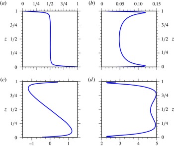
Height-resolved profiles of the mean (a), standard deviation (b), skewness (c) and kurtosis (d) of the temperature distribution for three-dimensional convection with periodic horizontal boundaries. The skewness and kurtosis are defined as the third and fourth standardised moment. Gaussian distributions have skewness of 0 and a kurtosis of 3.

In figure 2, the height-resolved mean, standard deviation, skewness and kurtosis of the temperature field are shown. As is well known, the mean temperature is almost constant in the bulk and has a steep gradient towards the hot and cold boundaries at $z=0$ and $z=1$ . The standard deviation takes its highest values close to the boundaries and decreases towards the centre of the bulk, indicating a temperature PDF that is broadening towards the boundaries. The height-resolved skewness takes its highest absolute values near the boundaries and decreases linearly as function of height in the bulk. This can be interpreted as hot fluid that is beginning to cool on its way from the lower to the upper plate (and vice versa). The kurtosis indicates that, apart from the boundaries, the temperature PDF is more peaked and shows stronger tails than the Gaussian distribution.

When the simplifications resulting from the statistical symmetries are incorporated into the general framework presented in § 2, (2.2) defining the PDF becomes

(3.1) $$\begin{eqnarray}\frac{\partial }{\partial z}(\langle u_{z}\mid T,z\rangle f)=-\frac{\partial }{\partial T}(\langle {\rm\Delta}T\mid T,z\rangle f),\end{eqnarray}$$

while the vector field (2.3) of the characteristics reads

(3.2) $$\begin{eqnarray}\left(\begin{array}{@{}c@{}}{\dot{T}}\\ {\dot{z}}\end{array}\right)=\left(\begin{array}{@{}c@{}}\langle {\rm\Delta}T\mid T,z\rangle \\ \langle u_{z}\mid T,z\rangle \end{array}\right).\end{eqnarray}$$

The PDF and the characteristic curves are therefore defined by the conditional averages of vertical velocity and heat diffusion. The next step is to estimate the conditional averages from the numerics while taking the statistical symmetries into account. Subsequently, the characteristics are obtained by integrating (3.2) for arbitrary initial conditions $(T_{0},z_{0})^{\text{T}}$ in phase space. Clearly, only initial conditions where the PDF and the conditional averages are defined, i.e. where there have been any events at all, can be considered.

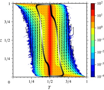
When integrating the characteristics for many starting positions, we observe that they tend to converge to what at first seems to be similar to a limit cycle. This cycle is shown in figures 5 and 6; we will later return to the description of the dynamics and behaviour of Rayleigh–Bénard convection that these figures offer. In contrast to a limit cycle, however, one would expect the characteristics to form concentric closed curves: to see this, let the phase space be densely seeded by the conditional particles described in § 2.2. As the density of the conditional particles following the characteristics is proportional to the temperature PDF, and a limit cycle acts as an attractor for the conditional particles, the temperature PDF should converge towards a ${\it\delta}$ -function that is non-vanishing on the cycle and zero everywhere else. This in turn stands in contrast to the fact that we are considering statistically stationary systems and that the temperature PDF is clearly not a ${\it\delta}$ -function, and thus it follows that the characteristics cannot converge to a limit cycle but must form concentric closed curves.

We find that the observed convergence is caused by the flawed conditionally averaged vector field estimated from the numerics by a binning process. The noise inherent to the binning violates the solenoidality of the probability flux (phase space velocity times PDF) as demanded by (3.1), and thus the imperfect binned vector field contains many localised sinks where the characteristics converge.

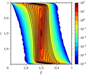
By smoothing the binned data through a convolution with a Gaussian kernel and projecting the vector field onto the solenoidal part (i.e. enforcing the validity of (3.1)), we are indeed able to find the expected concentric closed curves, as exemplified in figure 3. Here the horizontal axis corresponds to the temperature coordinate $T$ and the vertical axis to the vertical coordinate $z$ of the phase space; the background colour coding gives the temperature PDF $f(T,z)$ . For every starting point located on the $z=0.5$ -axis, the characteristics perform a closed loop in the counter-clockwise direction which shows how particles on average evolve through phase space. By tracing its course, one is able to reconstruct the typical Rayleigh–Bénard cycle a conditional particle undergoes. A fluid element near the lower plate first heats up and then starts to move up towards the cold plate. During its upward travel, it slowly cools and then becomes much colder when it is close to the top plate before it falls again towards the lower plate while beginning to heat up and starting what we term the RB cycle again. The cycles for fluid starting at more moderate temperatures (i.e. near $T=0.5$ ) show a smaller amplitude in both $T$ - and $z$ -direction. We do not find closed circles located further outwards, because the characteristics would visit areas of the phase space where no events are recorded in the numerics, and thus where the vector field is undefined. This usually happens near the vertical boundaries of the phase space (i.e. near the plates) where the support of the vector field becomes very narrow. Furthermore, we remark that the precise appearance of the closed cycles slightly varies with the parameters of the post-processing described above (e.g. the amount of smoothing); nevertheless, the description of the qualitative behaviour is found to be robust.

Figure 3.

Concentric closed characteristics found for three-dimensional convection after removing the imperfections from the binned conditionally averaged vector field, cf. text. The temperature PDF $f(T,z)$ is colour coded.

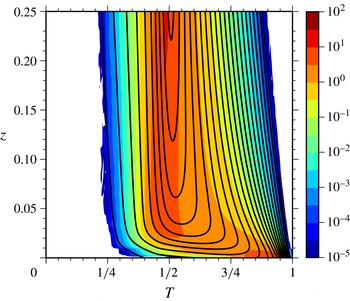
Without the aforementioned projection to keep the vector field solenoidal in the presence of noise, the characteristics converge in some parts of the phase space. To study this behaviour, and also the near-wall regions, we seed characteristics on the $\{T>0.5,z=0.5\}$ -line and integrate them backwards in time, as shown in figure 4. The comparison of the characteristics in the regions $T<0.5$ and $T>0.5$ immediately reveals the convergence for the non-solenoidal case, because the density of the characteristics on the right side (i.e. at later times) is higher than on the left side. Furthermore, the characteristics on the far right enter the boundary at $z=0$ when integrated backwards in time, or in other words, the characteristics leave the boundaries very close to each other and then become less dense with time. This corresponds to the fact that at $z=0$ , the temperature PDF becomes a ${\it\delta}$ -function located at $T=1$ due to the Dirichlet boundary condition. In fact, the characteristics should end precisely in this point, but this behaviour is not resolved here. Likewise, by symmetry considerations, the characteristics approaching the boundary from the far left side should also enter the point $\{T=1,z=0\}$ , which we do not observe. We speculate that a numerical resolution that goes beyond that demanded by the criterion of Shishkina et al. (Reference Shishkina, Stevens, Grossmann and Lohse2010) may be needed to capture the correct behaviour of the characteristics in this singular region of phase space.

Figure 4.

Characteristics seeded on the $\{T>0.5,z=0.5\}$ -line and followed backwards in time for three-dimensional convection. A zoom into the bottom region $0\leqslant z\leqslant 0.25$ is shown. The divergences of the vector field have not been removed here. The temperature PDF $f(T,z)$ is colour coded.

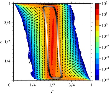
The cycle to which the characteristics converge in the presence of noise is shown in figure 5. This cycle is very similar to the closed curves shown in figure 3; in fact, it is almost completely embedded between two adjacent closed curves. While the solenoidal projection helps to find the required closed curves, the conditionally averaged vector field still containing the noise gives the same general picture of the RB cycle. Additionally, while removing divergences, the projection may introduce unpredictable systematic errors, especially in regions of the phase space where the support of the conditional averages and the PDF changes rapidly. Therefore, as we wish to focus on the qualitative features of Rayleigh–Bénard convection that the RB cycle as well as the vector field represent, we will from now on only consider the cases without the solenoidal projection and use the found cycle as one generic representative of the family of closed concentric curves. The same applies to the convection cases discussed in §§ 3.2 and 3.3 where the characteristics also tend to converge due to imperfections induced by noise.

Figure 5.

RB cycle of the characteristics for three-dimensional convection. The phase space speed along the cycle shown as solid thick line is coded in black (low speed) and white (high speed), i.e. the norm of the phase space velocity appearing in (3.2). The colour coding in the background shows the temperature PDF $f(T,z)$ . The arrows show the phase space velocity field, where the length of the arrows has been rescaled to arbitrary units for visualisation purposes. Note that around the lower-left and upper-right corners, no events were recorded (e.g. there is no fluid of temperature $T\approx 1$ near the upper plate).

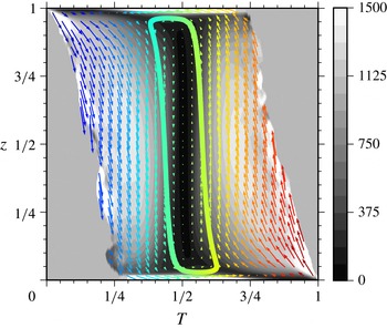
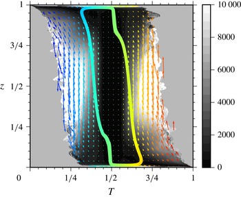
We now come back to the discussion of the qualitataive features that the conditionally averaged phase space velocity and the RB cycle describe. In figure 5, the RB cycle is shown together with the temperature PDF and in figure 6 together with the phase space velocity. From the first-mentioned figure, it is interesting to see that hot fluid on the RB cycle has the highest phase space speed in the range $0.25<z<0.5$ , i.e. hot rising fluid is fastest in the lower half of the convection vessel, and likewise for cold fluid in the upper half due to the up-down symmetry of Rayleigh–Bénard convection. Henceforth, wherever we describe a fluid process, the reversed process – interchanging hot $\leftrightarrow$ cold, bottom $\leftrightarrow$ top, up $\leftrightarrow$ down etc. – is also implied.

Figure 6.

RB cycle of the characteristics for three-dimensional convection as function of height and temperature. The colour of the arrows (with blue corresponding to $T=0$ and red to $T=1$ ) indicates the temperature. The black and white background colour shows the phase space speed.

The temperature PDF in figure 5 shows that the temperature distribution changes with the vertical coordinate and contracts to a ${\it\delta}$ -function at the fixed temperature boundaries. Furthermore, one can map the shape of the distribution to the higher moments in figure 2, i.e. the peaks of the standard deviation near the boundaries and the linear dependence of the skewness on the height in the bulk region. We note that the isocontours of the PDF do not lie tangent to the vector field or the RB cycle because the divergence the phase space velocity, $(\partial /\partial z)\langle u_{z}\mid T,z\rangle +(\partial /\partial T)\langle {\rm\Delta}T\mid T,z\rangle$ , is non-vanishing.

In figure 6, the black and white background colour corresponds to the phase space speed, and the temperature is given by the colour of the arrows. This display allows us to identify how fluid behaves in different parts of the phase space. Near the boundaries, fluid of all temperatures displays high phase space speeds, while in the bulk, only fluid of intense temperature (i.e. deviating strongly from the mean) has high speeds. This supports the previous finding that hot fluid on the RB cycle has its highest speed in the lower half. Fluid that has the mean temperature (cf. figure 2 a) is found to be at rest because no buoyancy acts on it and it does not heat up or cool down. As can be expected a priori, the vector field shows that the main movement in the $T$ -direction, i.e. heating and cooling, takes place near the boundaries, while the main movement in the vertical direction happens in the bulk.

3.2. Two-dimensional convection with periodic horizontal boundaries

The next case we investigate is that of two-dimensional Rayleigh–Bénard convection with periodic horizontal boundaries. The parameters are $\mathit{Ra}=5\times 10^{8}$ , $\mathit{Pr}=1$ and ${\it\Gamma}=4$ , and the numerical scheme used is identical to that of § 3.1. Again, the two horizontal plates are no-slip walls of fixed temperature. The numerical resolution is $1536\times 384$ equidistant grid points with 7 grid points in the vertical direction falling into the boundary layers (cf. Shishkina et al. Reference Shishkina, Stevens, Grossmann and Lohse2010), and the ensemble consists of 3891 snapshots separated by 3.75 free-fall time units.

Figure 7.

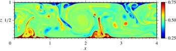
Temperature field for two-dimensional convection with periodic horizontal boundary conditions. The colour scale for $T$ is shown on the right.

A snapshot of the temperature field is shown in figure 7, and one can see coherent structures in the form of four plume hot spots (two at the top, two at the bottom) and four convection rolls, even at this intermediate Rayleigh number. Also, localised round blobs of hot and cold fluid can be observed. The statistical symmetries in this system are identical to the ones for the three-dimensional periodic case discussed previously, which means that the phase space becomes two-dimensional and the statistics depend on $T$ and $z$ only.

Figure 8.

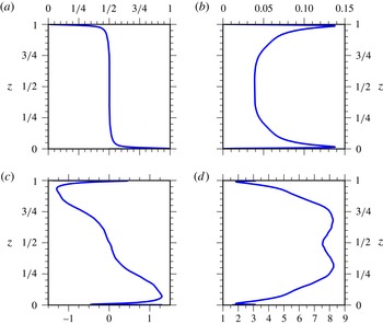
First four standardised moments of temperature for two-dimensional convection, analogous to figure 2: (a) mean; (b) standard deviation; (c) skewness; (d) kurtosis.

Figure 8 shows the first four height-resolved standardised moments of temperature. While the mean temperature profile has the same shape as the one from three-dimensional convection (cf. figure 2), the higher moments show subtle new features. For the three-dimensional case, the moment profiles as a function of the height are smoother than for the two-dimensional case. Especially, the skewness shows transitions and is not as linear in the bulk as for the three-dimensional case. We link this to the coherent structures in the form of plume hot spots in the two-dimensional case because the position of the transitions in the moments corresponds to the vertical size of the plume hot spots (cf. figure 7). In the plume hot spots, there is a recycling of hot fluid, which means that fluid that is hotter than the mean temperature profile is trapped near the hot bottom plate for some time instead of being advected upwards directly, cf. Sugiyama et al. (Reference Sugiyama, Ni, Stevens, Chan, Zhou, Xi, Sun, Grossmann, Xia and Lohse2010). This hot trapped fluid causes a temperature distribution that is strongly skewed towards higher temperatures near the lower plate. Above the hot spot, only a sharp jet of hot fluid remains, which results in a flatter profile of the skewness. In three-dimensional convection, the trapping mechanism of plume hot spots is missing: In general terms, with three-dimensional convection there is another lateral dimension into which the fluid can escape and be advected away, forming the sheet-like plumes that can also be found in figure 1 (Schmalzl et al. (Reference Schmalzl, Breuer, Wessling and Hansen2004) and van der Poel et al. (Reference van der Poel, Stevens and Lohse2013) also discuss differences in flow structures between two- and three-dimensional convection). Therefore, the entrapment seen in two-dimensional convection does not occur in three dimensions, which means that a strong mechanism that in two dimensions traps hot fluid near the bottom is missing for the three-dimensional case.

Figure 9.

RB cycle of the characteristics for two-dimensional convection, together with the temperature PDF. Illustration analogous to figure 5.

Figure 10.

RB cycle of the characteristics for two-dimensional convection, together with the phase space speed. Illustration analogous to figure 6.

When we estimate the conditional averages for two-dimensional convection from the simulation and then numerically calculate the characteristics, we again find that the dynamics in phase space resemble a closed cycle. This RB cycle is shown in figures 9 and 10. While the RB cycle displays the same basic cycle of fluid heating up at the bottom, moving upwards, cooling down at the top plate and falling down again, there are some differences when compared to the three-dimensional case (figures 5 and 6).

The most striking new feature is a kink in the RB cycle in the lower left and upper right corners. As can be seen from the colour coding of the cycle, this is also the region of the lowest phase space speed. Therefore, we also link this region to the recycling areas discussed above because fluid trapped in the plume hot spots undergoes almost no net vertical movement and needs more time to heat up in comparison to fluid that is in direct contact with the much hotter bottom plate. A similar argument has been discussed by van der Poel et al. (Reference van der Poel, Stevens and Lohse2013).

Another difference compared to the three-dimensional case is that there is a bulge in the temperature PDF towards higher temperatures (around $T\approx 0.6$ , $z\approx 0.15$ ). This bulge is due to the hotter-than-average fluid that gathers near the bottom plate and is therefore compatible with the interpretation of the recycling fluid discussed above. Also, this bulge gives a direct impression of the high skewness values found in this region (cf. figure 8).

Figure 10 shows the vector field of the phase space velocities together with its norm (coded in black and white). The phase space velocities are more heterogeneously distributed when compared to the three-dimensional case, e.g. the high speeds in the bulk for intense temperatures are more pronounced (cf. figure 5). These strong vertical movements in the bulk lead to higher phase space speeds compared to the case of three dimensions (see the colour scale in figures 6 and 10). We believe this can only in part be attributed to the difference in Rayleigh numbers ( $2.4\times 10^{7}$  versus  $5\times 10^{8}$ ), but is also due to the coherent structures found in two dimensions, i.e. plume hot spots as localised events of intense temperature. It is also found that in the kink region the RB cycle passes through the region of lowest phase space speed, which can be understood as the average dynamics being slowed down in the recirculating plume hot spots.

3.3. Three-dimensional convection in cylindrical vessel

The last Rayleigh–Bénard geometry under investigation is a closed cylindrical vessel. The control parameters are $\mathit{Ra}=2\times 10^{8}$ , $\mathit{Pr}=1$ and ${\it\Gamma}=1$ (diameter over height). All the walls are no-slip, and the horizontal plates are of constant temperature while the sidewalls are thermally insulating. The ensemble consists of $870$ snapshots that are obtained from direct numerical simulation using a second-order finite difference scheme on a staggered cylindrical grid (Verzicco & Camussi Reference Verzicco and Camussi2003) with a resolution of $N_{{\it\varphi}}\times N_{r}\times N_{z}=384\times 192\times 384$ grid points (with ${\it\varphi}$ , $r$ and $z$ being the azimuthal, radial and vertical coordinates, respectively). The boundary layer contains $17$ grid points in the vertical direction. 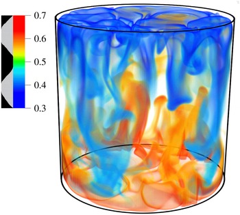The snapshots are separated by $1$ free-fall time unit. Figure 11 shows a snapshot of the temperature field.

Figure 11.

Snapshot of the temperature field in three-dimensional Rayleigh–Bénard convection in a ${\it\Gamma}=1$ -cylinder. In the upper left corner, the colour and opacity scale is shown; fluid around the mean temperature is translucent.

Rayleigh–Bénard convection in a cylinder has statistical symmetries that are different from the former two cases of horizontally homogeneous convection. In addition to the temperature $T$ and vertical position $z$ , the statistics now also depend on the radial position $r$ in the cylinder. Here $r=0$ corresponds to the cylinder axis and the sidewall is at $r=1/2$ .

Figure 12.

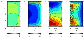
First four standardised $r$ – $z$ -resolved moments of the temperature distribution, i.e. (a) mean value, (b) standard deviation, (c) skewness and (d) kurtosis. Here the convection is in a cylinder with ${\it\Gamma}=1$ .

In figure 12 the $r$ – $z$ -resolved first four standardised moments of the temperature distribution are shown. The horizontal and vertical axes correspond to the radial coordinate $r$ and the vertical coordinate $z$ , respectively. The mean temperature profile is almost constant in the bulk, and only near the hot and cold plate (and to a lesser extent near the sidewalls) can a deviation be seen. As with the former cases, the standard deviation of the temperature takes its highest values near the horizontal plates and falls off towards the middle of the convection cell with a local minimum at $z=0.5$ . Also, it can be seen that this local minimum is less pronounced near the sidewalls, i.e. for high $r$ . After rising to its maximum value at $z\approx 0.1$ , the skewness varies monotonically with increasing $z$ . This has also been found for the former two cases. Regarding the radial dependence, the skewness falls off towards the sidewalls, indicating a less asymmetric temperature distribution there, while its highest values are found near the cylinder axis. Although the statistics are less converged for the kurtosis (especially near $r=0$ due to the cylindrical geometry), one can see that the highest values correspond roughly to the extrema of the skewness. These high values of skewness and kurtosis near the bottom wall can be attributed to hot localised plumes detaching from the hot bottom plate and piercing into the colder fluid of the bulk. We also note that the absolute values of skewness and kurtosis are higher than in the former two cases (figures 2 and 8), which can be understood on dimensional grounds: in horizontally periodic convection, we averaged over all horizontal directions and therefore averaged out the sharp maxima that can be seen in the cylindrical case (figure 12) where the statistics are resolved additionally in the horizontal coordinate $r$ .

When inserting the temperature PDF $f(T,r,z)$ and the conditional averages $\langle \cdot \mid T,r,z\rangle$ into the general framework from § 2, the PDF defining equation (2.2) becomes

(3.3) $$\begin{eqnarray}\frac{1}{r}\frac{\partial }{\partial r}(r\langle u_{r}\mid T,r,z\rangle f)+\frac{\partial }{\partial z}(\langle u_{z}\mid T,r,z\rangle f)=-\frac{\partial }{\partial T}(\langle {\rm\Delta}T\mid T,r,z\rangle f),\end{eqnarray}$$

while the characteristics (2.3) read

(3.4) $$\begin{eqnarray}\left(\begin{array}{@{}c@{}}{\dot{T}}\\ {\dot{r}}\\ {\dot{z}}\end{array}\right)=\left(\begin{array}{@{}c@{}}\langle {\rm\Delta}T\mid T,r,z\rangle \\ \langle u_{r}\mid T,r,z\rangle \\ \langle u_{z}\mid T,r,z\rangle \end{array}\right).\end{eqnarray}$$

In comparison to the former two cases, we now deal with a three-dimensional phase space where the additional dimension is related to the radial movement. From (3.4) one sees that the radial coordinate $r$ of the characteristics evolves according to the conditional average of radial velocity $u_{r}$ .

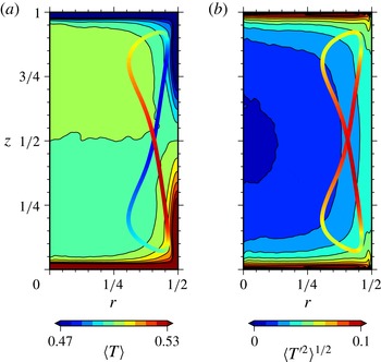
We now again turn to the integration of the characteristics, following (3.4). Although cylindrical convection is intrinsically different from the former two cases of horizontally periodic convection (due to three- versus two-dimensional phase space), we still find that the average dynamics of fluid parcels are described by a closed, twisted loop in phase space that shares common features with the former two. The cycle is shown in figures 13 and 14 as the slender figure eight shaped curve.

Figure 13.

RB cycle of the characteristics for convection in a ${\it\Gamma}=1$ -cylinder. (a) Temperature of the cycle (figure eight) and $r$ – $z$ -resolved mean temperature colour coded. (b) The $r$ – $z$ -resolved standard deviation of temperature where $T^{\prime }=T-\langle T\rangle$ . The colour of the figure eight shaped cycle indicates its absolute temperature difference with respect to the background temperature.

Figure 14.

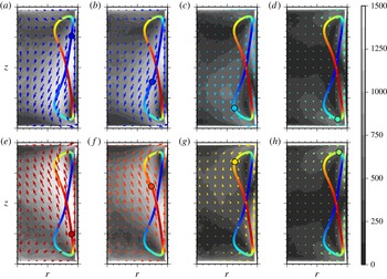
Vector field governing the characteristics in phase space for convection in a ${\it\Gamma}=1$ -cylinder, cf. (3.4). Extents of horizontal and vertical axes as in figure 13, i.e.  $0\leqslant r\leqslant 1/2$ and $0\leqslant z\leqslant 1$ . The RB cycle is the slender figure eight shaped curve at the right side. The temperature of the vector field and the RB cycle is colour coded as in figure 13(a), and the phase space speed (i.e. norm of velocity) is coded in black and white in the background (with white being high velocity). The eight panels (a–h) follow a fluid parcel (circle on the cycle, with the colour showing its temperature) along the RB cycle and show a slice of the vector field of the phase space velocity in the $r$ – $z$ plane at the $T$ coordinate of the fluid parcel (with $T\in \{0.475,0.478,0.487,0.495,0.525,0.519,0.509,0.501\}$ from (a) to (h)). The vector fields show the average movement in different regions of the convection cell of fluid of a particular temperature.

In figure 13(a), the background shows the mean temperature (cf. figure 12) and the figure eight shaped curve shows a projection of the RB cycle into the $r$ – $z$ -plane. The third coordinate of the RB cycle, the temperature $T$ , is colour coded. The temperature scale corresponds to the minimal and maximal temperature ( $T=0.47$ and $T=0.53$ ) the RB cycle takes. When tracing the cycle, one can again identify the Rayleigh–Bénard cycle of the horizontally periodic convection cases, superposed with an additional inwards and outwards motion: starting with fluid of mean temperature that is quickly heating up at the bottom, it then begins to rise up and move inwards into the bulk until $z\approx 0.8$ and $r\approx 0.3$ , where it goes outwards and starts to cool down. At the maximal $z$ , the fluid cools down quickly and then falls towards the lower plate while moving inwards, thus starting the RB cycle again. Additionally, one can see that the hot fluid rising from the lower plate steadily cools down when it crosses the bulk of almost uniform temperature; this is related to the monotonically decreasing skewness of temperature that can be seen in figure 12.

The difference of the temperature of the RB cycle and the background temperature (cf. colour coding of these two in figure 13 a) shows that the regions where the temperature of the RB cycle deviates most from the mean background temperature are the regions of high buoyancy and correspond to the regions of main vertical movement in the bulk. To elaborate on this, figure 13(b) shows the standard deviation of the temperature field in the background, and the colour coding of the cycle shows the absolute deviation of its temperature coordinate $T$ from the mean temperature. The deviation of the temperature of a fluid particle on the cycle from the surrounding mean temperature determines its mean buoyancy, thus panel (b) tells us how strong the buoyancy acts; the highest values for hot rising fluid are found in the lower half of the convection cell. In comparison, the mean deviation of fluid from the mean temperature profile (shown in the background as the standard deviation of temperature) is much weaker. To summarise, from figure 13(a) one can see in which direction the buoyancy acts, while figure 13(b) shows its strength.

The vector field of the characteristics is shown in figure 14. Due to the difficulty of displaying a vector field in three-dimensional phase space, we show slices of the phase space velocity in the $r$ – $z$ plane at different $T$ . Figure 14(a–h) shows one cycle of a fluid parcel travelling along the RB cycle, with its temperature colour coded as in figure 13(a). Additionally to the RB cycle described above, figure 14 also reveals the average behaviour of fluid in different parts of the convection cell, conditioned on its temperature. The arrows show an $r$ – $z$ slice of the vector field of the characteristics (3.4) at the $T$ coordinate of the cycle. Also, the black and white background colour indicates the phase space speed, i.e. how fast a fluid parcel travels through phase space (with white being the fastest movement). The arrows indicate the mean movement of fluid of a given temperature in different regions of the convection cell.

Panel (a) shows that cold fluid (here, $T=0.475$ ) has the highest speeds in the bulk and near the sidewall. Near the cold top plate, cold fluid is mainly transported towards the outer wall. For $z<0.75$ , the direction of movement is slightly tilted towards the cylinder axis. Cold fluid that falls down along the sidewall is deflected towards the inner cylinder at around $z\approx 0.25$ due to a corner flow that propels cold fluid upwards along the sidewall; notice that at $r\approx 0.45$ and $z\approx 0.25$ , up- and down-welling cold fluid collides. This feature can be understood as cold plumes that are formed at the upper plate and are swept towards the sidewalls. The plumes then fall down along the sidewall until they hit the hot fluid at the bottom plate where they are directed inwards. These cold plumes that fall down along the sidewall can also be seen in figure 11.

The fluid from panel (c) is less cold ( $T=0.487$ ) and has overall lower speeds, but still shows the same features as in panel (a), e.g. cold fluid is swept along the upper plate outwards and falls down along the sidewall until it hits the upwelling corner flow. The vector fields for fluid of mean temperature ( $T\approx 0.5$ , panel (d) and (h)) are symmetric around $z=0.5$ and show an almost vanishing velocity in the bulk. Near the horizontal plates, fluid is swept towards the sidewalls and from there vertically towards the $z=0.5$ -line.

The rest of the panels complete one run of the RB cycle and due to the up-down symmetry, contain the same information already described. Nonetheless, from all eight panels it can be seen that fluid for all temperatures has high phase space speed near the sidewalls, which can be attributed to plumes that are guided along the outer walls of the cylinder, and also has high speeds near the bottom and top plate which is due to the vigorous temperature contrast between fluid and horizontal plates that leads to high speeds regarding the $T$ coordinate. Further, we must stress here that the corner flows show up due to the investigation being conditioned on the temperature and not due to any large-scale structure that may be present in the fields; this structure is lost in the azimuthal averaging process when obtaining the vector field from (3.4). Therefore, in our analysis the corner flows are statistical structures that are not necessarily related to structures in the flow.