1 Introduction
The formation and dynamics of vortices in flow past sharp edges are of fundamental interest and have been a focus of research since the work of Prandtl (Anderson Reference Anderson2005). The present work is concerned with viscous flow past wedges.
Much research has been done on the limiting case of a flat plate, which corresponds to a wedge of zero angles. A partial list of these works includes Pierce (Reference Pierce1961), Hudson & Dennis (Reference Hudson and Dennis1985), Koumoutsakos & Shiels (Reference Koumoutsakos and Shiels1996), Luchini & Tognaccini (Reference Luchini and Tognaccini2002), Xu & Nitsche (Reference Xu and Nitsche2014, Reference Xu and Nitsche2015). However, the literature on flow past a wedge of non-zero angles is limited. The studies that are most closely related to the current work are those of Pullin (Reference Pullin1978) and Pullin & Perry (Reference Pullin and Perry1980). Pullin (Reference Pullin1978) studied vortex evolution at the edge of an infinite wedge using an inviscid self-similar vortex sheet model. The results showed the large-scale structure of the rolled-up sheet. In Pullin & Perry (Reference Pullin and Perry1980) (hereafter PP80), the authors visualized the starting vortex formed at the wedge edge in laboratory experiments and compared their observation with the inviscid self-similar results. Other works on flow past wedges include the work of Davies, Dakin & Falconer (Reference Davies, Dakin and Falconer1995), who numerically studied the interactions of coastal currents (uniform horizontal flow) with topographic indentations (a triangular headland). In this work, the Coriolis term was present in the equations of motion. Jespersen et al. (Reference Jespersen, Thomassen, Andersen and Bohr2004) investigated vorticity production behind a periodically oscillating triangular profile.
In the recent work of Xu & Nitsche (Reference Xu and Nitsche2014) and Xu & Nitsche (Reference Xu and Nitsche2015) (the latter is referred to as XN15 hereafter), viscous flow past a flat plate with accelerating background flow was studied numerically for a range of Reynolds numbers. The results were in good agreement with the experimental results of PP80 for thin wedges with an angle of
 $5^{\circ }$
and yielded further insight into details of vorticity evolution. The goal of this paper is to study vortex formation induced by the potential driving flow around a wedge of moderate angles. To avoid the effect of other external length scales, we consider flow past an infinite wedge.
The numerical method used here is an adaptation of the method for flow past a finite flat plate to an infinite wedge, as presented in Xu & Nitsche (Reference Xu and Nitsche2014). The Navier–Stokes equations are solved using a time-splitting method, in which the vorticity convection is treated using a semi-Lagrangian method, and the vorticity diffusion is solved using the Crank–Nicolson implicit scheme. In the latter case, a finite domain around the wedge is mapped conformally onto a rectangle. The finite difference scheme is applied in the mapped domain to solve the governing equations on a regular grid. The computational domain is chosen to be so large that all vorticity generated at the wall that contributes to the tip vortex is included.
The current study focuses on the formation of a starting vortex near the wedge tip at early and medium times. The computation reveals new and detailed information about vorticity evolution at a wedge with non-zero angles. Hierarchical vorticity regions of alternate signs are observed. The primary starting vortex contains positive vorticity. A negative vorticity region appears within the primary one at some positive time. Another positive vorticity region appears within the negative one later. The appearance time for the negative vorticity region monotonically increases with the wedge angle, whereas for the positive vorticity region within, the appearance time decreases first and then increases with an increasing wedge angle. In association with these vorticity regions of alternate signs, multiple recirculating regions in the streamlines are formed. Streaklines are computed by releasing fluid particles at the wedge tip. A kink in the streaklines is observed near the edge. The starting vortex contains a local vorticity maximum, the vortex centre. The observed scaling behaviour of the vortex centre trajectory and vorticity is reported, and compared with that available in laboratory experiments and the inviscid similarity theory.
The paper is organized as follows. Section 2 describes the problem considered and the numerical method used. Section 2.1 provides the governing equations and non-dimensional variables. Sections 2.2–2.4 present the time-splitting method, the computational domain and the convergence study, respectively. Section 3 shows the numerical results. Section 4 provides a summary.
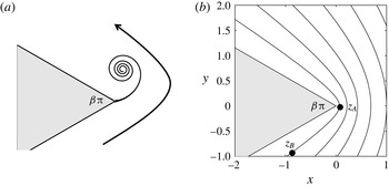
(a) Problem description of flow past a wedge. The wedge angle is
 ${\it\beta}{\rm\pi}$
. (b) Selected streamlines of the potential flow. Two points,
 $\boldsymbol{z}_{A}$
and
 $\boldsymbol{z}_{B}$
, are chosen, and they are used later to determine the size of the computational domain.

2 Problem formulation and numerical method
2.1 Problem description
Figure 1(a) illustrates the problem considered. An infinite wedge is immersed in a viscous fluid flow. The flow is driven by the potential flow around a wedge given by the streamfunction
 $$\begin{eqnarray}\displaystyle {\it\psi}_{\infty }(\boldsymbol{z})=\text{Im}(-\text{i}az^{1/(2-{\it\beta})}), & & \displaystyle\end{eqnarray}$$
where
 ${\it\beta}{\rm\pi}$
is the wedge angle,
 $z=x+\text{i}y$
and
 $\boldsymbol{z}=(x,y)$
are the coordinates. The wedge is symmetric about
 $y=0$
with the tip located at the origin. Streamlines of the potential flow are shown in figure 1(b). This figure is also used later to discuss the size of the computational domain in § 2.3.
The Navier–Stokes equations are written in the vorticity-streamfunction formulation (
 ${\it\omega}{-}{\it\psi}$
)
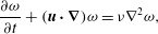 $$\begin{eqnarray}\displaystyle & \displaystyle \frac{\partial {\it\omega}}{\partial t}+(\boldsymbol{u}\boldsymbol{\cdot }\boldsymbol{{\rm\nabla}}){\it\omega}={\it\nu}{\rm\nabla}^{2}{\it\omega}, & \displaystyle\end{eqnarray}$$
 $$\begin{eqnarray}\displaystyle & \displaystyle {\rm\nabla}^{2}{\it\psi}=-{\it\omega}\quad \text{with }{\it\psi}=0\text{ on }S\text{ and }{\it\psi}\rightarrow {\it\psi}_{\infty }\text{as }|\boldsymbol{z}|\rightarrow \infty , & \displaystyle\end{eqnarray}$$
 $$\begin{eqnarray}\displaystyle & \displaystyle \boldsymbol{u}={\rm\nabla}^{\bot }{\it\psi}\quad \text{with }\boldsymbol{u}=\mathbf{0}\text{ on }S. & \displaystyle\end{eqnarray}$$
 $S$
is the solid wedge boundary,
 ${\rm\nabla}^{\bot }{\it\psi}=(\partial {\it\psi}/\partial y,-\partial {\it\psi}/\partial x)$
, and
 $\boldsymbol{u}$
is the velocity vector. All variables in the Navier–Stokes equations are dimensional. The units are time
 $t~(\text{s})$
, velocity
 $\boldsymbol{u}~(\text{m}~\text{s}^{-1})$
, vorticity
 ${\it\omega}~(1~\text{s}^{-1})$
and kinematic viscosity
 ${\it\nu}~(\text{m}^{2}~\text{s}^{-1})$
. Hereafter, these units will not be repeated in the text and figures to avoid redundancy.
It is noted that the infinite wedge has no length scale. One possible non-dimensionalization is given in Luchini & Tognaccini (Reference Luchini and Tognaccini2002). This paper follows PP80 (below equation (7a,b), p. 245) and introduces the scale Reynolds number
 $$\begin{eqnarray}\displaystyle Re_{s}(t)=\frac{a^{2/(2-n_{0})}t^{2/(2-n_{0})-1}}{{\it\nu}}\quad \text{with }n_{0}=\frac{1}{2-{\it\beta}}. & & \displaystyle\end{eqnarray}$$
As noted by PP80, there is an internal-implicit length
 $$\begin{eqnarray}\displaystyle L=a^{1/(2-n_{0})}t^{1/(2-n_{0})}. & & \displaystyle\end{eqnarray}$$
Therefore, the scale Reynolds number can also be written as
 $Re_{s}(t)=L^{2}/t{\it\nu}$
. Only the case of an impulsively started flow is considered in the current study. The computations are performed with
 $a=1$
and
 ${\it\nu}=0.002$
unless otherwise noted.
The dimensionless variables are indicated with a hat, e.g.
 $\hat{x}=x/L$
,
 $\hat{y}=y/L$
,
 $\hat{{\it\omega}}={\it\omega}t$
, etc. Following PP80, we choose to show the convergence study, contour plots of vorticity, streamlines and streaklines in dimensional variables. When it comes to the scaling behaviour of the vorticity and trajectory of the vortex centre, the dimensionless scale Reynolds number
 $Re_{s}$
is used since it is the appropriate way to present the results.
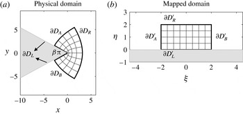
Schematic plots of (a) the physical domain (
 $z$
-plane) and (b) the mapped domain (
 ${\it\zeta}$
-plane). The two domains are related by (2.5). Four corresponding boundaries of the mesh are labelled in both domains.

2.2 Numerical method
The Navier–Stokes equations are solved in two domains, as illustrated in figure 2. One is the physical domain (or
 $z$
-plane) with coordinates
 $(x,y)$
and the other is a mapped domain (or
 ${\it\zeta}$
-plane) with coordinates
 $({\it\xi},{\it\eta})$
. They are related via the conformal mapping
 $$\begin{eqnarray}\displaystyle z=\text{i}{\it\zeta}^{1/(2-{\it\beta})}\quad \text{with }z=x+\text{i}y\text{ and }{\it\zeta}={\it\xi}+\text{i}{\it\eta}. & & \displaystyle\end{eqnarray}$$
In figure 2, it is seen that a fan-shaped area in the
 $z$
-plane is transformed onto a rectangle in the
 ${\it\zeta}$
-plane. The wedge edge is transformed into a horizontal line. The four boundaries of the finite fan are denoted by
 $\partial D_{L}$
,
 $\partial D_{B}$
,
 $\partial D_{R}$
and
 $\partial D_{A}$
. The corresponding boundaries in the
 ${\it\zeta}$
-plane are shown in figure 2(b). A uniform mesh grid is used in the
 ${\it\zeta}$
-plane, and this yields a natural refinement near the wedge tip in the
 $z$
-plane. The grid size is large in the figure for illustration. The deformation matrix
 $\unicode[STIX]{x1D645}$
is computed as
 $$\begin{eqnarray}\displaystyle \unicode[STIX]{x1D645}=\left(\begin{array}{@{}cc@{}}\displaystyle \frac{\partial {\it\xi}}{\partial x} & \displaystyle \frac{\partial {\it\xi}}{\partial y}\\ \displaystyle \frac{\partial {\it\eta}}{\partial x} & \displaystyle \frac{\partial {\it\eta}}{\partial y}\end{array}\right)\quad \text{and}\quad \unicode[STIX]{x1D645}^{-1}=\left(\begin{array}{@{}cc@{}}\displaystyle \frac{\partial x}{\partial {\it\xi}} & \displaystyle \frac{\partial x}{\partial {\it\eta}}\\ \displaystyle \frac{\partial y}{\partial {\it\xi}} & \displaystyle \frac{\partial y}{\partial {\it\eta}}\end{array}\right). & & \displaystyle\end{eqnarray}$$
 $|\unicode[STIX]{x1D645}|$
is the determinant or the Jacobian.
The Navier–Stokes equations are solved using a time-splitting scheme. Xu & Nitsche (Reference Xu and Nitsche2014) implemented the method to simulate viscous flow past a finite flat plate. In the current study, the method is modified for the wedge, and the computational procedure is outlined below.
The mapped domain
 $D$
is a rectangular box
 $$\begin{eqnarray}\displaystyle D=[{\it\xi}_{min},{\it\xi}_{max}]\times [{\it\eta}_{min},{\it\eta}_{max}]. & & \displaystyle\end{eqnarray}$$
The box is partitioned by
 $(N_{{\it\xi}}+1)\times (N_{{\it\eta}}+1)$
equally spaced grid points,
 $({\it\xi}_{j},{\it\eta}_{k})$
, where
 $$\begin{eqnarray}\displaystyle {\it\xi}_{j}=jh,\quad j=0,\ldots ,N_{{\it\xi}},\quad {\it\eta}_{k}=kh,\quad k=0,\ldots ,N_{{\it\eta}}, & & \displaystyle\end{eqnarray}$$
with
 $h$
the mesh size.
 $N_{{\it\xi}}$
and
 $N_{{\it\eta}}$
are chosen so that
 $h=({\it\xi}_{max}-{\it\xi}_{min})/N_{{\it\xi}}=({\it\eta}_{max}-{\it\eta}_{min})/N_{{\it\eta}}$
. The time is discretized as
 $$\begin{eqnarray}\displaystyle t_{n}=n{\rm\Delta}t,\quad n=0,\ldots ,N,{\rm\Delta}t=t_{f}/N, & & \displaystyle\end{eqnarray}$$
where
 $t_{f}$
is the final time. All fluid variables are solved on the grid point; for example,
 ${\it\omega}_{j,k}^{n}$
approximates
 ${\it\omega}({\it\xi}_{j},{\it\eta}_{k},t_{n})$
.
The vorticity at
 $t_{n+1}$
is obtained in two sub-steps.
Step 1. In the physical domain, the interior vorticity is convected by solving
 $$\begin{eqnarray}\displaystyle \frac{\text{D}Q}{\text{D}t}=0,\quad \text{subject to }Q(t_{n})={\it\omega}^{n}, & & \displaystyle\end{eqnarray}$$
using a semi-Lagrangian method. This provides an intermediate value of vorticity
 ${\it\omega}^{\ast }=Q(t_{n+1})$
.
Step 2. In the mapped domain, the interior vorticity is diffused by solving the equation
 $$\begin{eqnarray}\displaystyle \frac{\partial Q}{\partial t}=\frac{{\it\nu}}{|\unicode[STIX]{x1D645}^{-1}|}{\rm\nabla}_{{\it\xi},{\it\eta}}^{2}Q,\quad \text{with }Q(t_{n})={\it\omega}^{\ast }. & & \displaystyle\end{eqnarray}$$
Then, set
 ${\it\omega}^{n+1}=Q(t_{n+1})$
. Here,
 ${\rm\nabla}_{{\it\xi},{\it\eta}}^{2}Q=\partial ^{2}Q/\partial {\it\xi}^{2}+\partial ^{2}Q/\partial {\it\eta}^{2}$
is evaluated in the mapped domain. A second-order Crank–Nicolson implicit scheme is applied in both space and time.
The streamfunction
 ${\it\psi}^{n+1}$
in the interior domain is obtained by solving the Poisson equation (2.2b
). The boundary values of the streamfunction are obtained by integrating all non-zero vorticity in the domain with the domain-specific Green’s function
 $$\begin{eqnarray}\displaystyle G_{S}(\boldsymbol{z},\boldsymbol{z}_{0})=-\frac{1}{2{\rm\pi}}\log \left|\frac{\text{i}z^{1/(2-{\it\beta})}-\text{i}z_{0}^{1/(2-{\it\beta})}}{\text{i}z^{1/(2-{\it\beta})}-(\text{i}z_{0}^{1/(2-{\it\beta})})^{\ast }}\right|, & & \displaystyle\end{eqnarray}$$
where
 $z=x+\text{i}y$
,
 $z_{0}=x_{0}+\text{i}y_{0}$
, and
 $\ast$
denotes the complex conjugate. Boundary vorticity values are obtained from the updated streamfunction by enforcing the no-slip boundary condition. The boundary vorticity, including the wedge tip, is computed as
 $$\begin{eqnarray}{\it\omega}_{bd}^{n+1}=-\frac{1}{|\unicode[STIX]{x1D645}^{-1}|}\frac{\partial ^{2}{\it\psi}^{n+1}}{\partial {\it\eta}^{2}}.\end{eqnarray}$$
The vorticity values are zero on the incoming boundary
 $\partial D_{B}^{\prime }$
, and the vorticity values on the outgoing boundary
 $\partial D_{A}^{\prime }$
are extrapolated from the interior domain. The velocity components,
 $(u^{n+1},v^{n+1})$
, are computed in the mapped domain using the chain rule
 $$\begin{eqnarray}\displaystyle & \displaystyle u^{n+1}=\frac{\partial {\it\psi}^{n+1}}{\partial y}=\frac{\partial {\it\psi}^{n+1}}{\partial {\it\xi}}\frac{\partial {\it\xi}}{\partial y}+\frac{\partial {\it\psi}^{n+1}}{\partial {\it\eta}}\frac{\partial {\it\eta}}{\partial y}, & \displaystyle\end{eqnarray}$$
 $$\begin{eqnarray}\displaystyle & \displaystyle v^{n+1}=-\frac{\partial {\it\psi}^{n+1}}{\partial x}=-\frac{\partial {\it\psi}^{n+1}}{\partial {\it\xi}}\frac{\partial {\it\xi}}{\partial x}-\frac{\partial {\it\psi}^{n+1}}{\partial {\it\eta}}\frac{\partial {\it\eta}}{\partial x}. & \displaystyle\end{eqnarray}$$
The streaklines are visualized by placing fluid particles in the flow and letting them move at the fluid velocity. In the computation, nine particles are placed along the edge near the tip at every time step. A second-order Adams–Bashforth scheme is applied to compute the positions of these particles.
Determining the size of the computational domain. The wedge angle is
 ${\it\beta}{\rm\pi}$
. Locations of
 $\boldsymbol{z}_{A}$
and
 $\boldsymbol{z}_{B}$
in the physical domain are illustrated in figure 1(b).
2.3 Size of the computational domain and parameters
The flow is computed up to some final time
 $t_{f}$
. The domain size is chosen so that particles initially placed on the domain boundary, below the wedge and travelling in the potential flow for a time interval
 $0<t<t_{f}$
, do not reach the wedge tip. Specifically, they do not reach
 $y=0$
. This criterion ensures that all wall-generated vorticity that ends up in the vortex by time
 $t_{f}$
is accounted for. Details on determining the domain size are provided below.
We choose a point
 $A$
near the tip, located at
 $\boldsymbol{z}_{A}$
as shown in figure 1(b), and a point
 $B$
somewhere below the wedge at
 $\boldsymbol{z}_{B}$
. Particles released at
 $\boldsymbol{z}_{B}$
, travelling at the potential flow velocity, will reach
 $\boldsymbol{z}_{A}$
. Given the final or travelling time
 $t_{f}$
and
 $\boldsymbol{z}_{A}$
, we solve for
 $\boldsymbol{z}_{B}$
. The computed value of
 $\boldsymbol{z}_{B}$
is used to determine the location of the right boundary
 $\partial D_{B}^{\prime }$
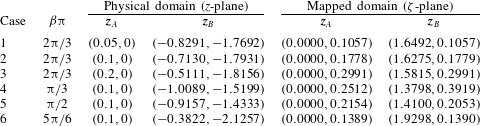
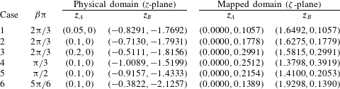
in the mapped domain. Table 1 lists pairs of
 $\boldsymbol{z}_{A}$
and
 $\boldsymbol{z}_{B}$
in both the physical and mapped domains at the final time
 $t_{f}=2.5$
. In table 1, cases 1–3 are for a fixed wedge angle of
 ${\it\beta}{\rm\pi}=2{\rm\pi}/3$
and three different locations of
 $\boldsymbol{z}_{A}$
on
 $y=0$
,
 $x=0.05,0.1,0.2$
; cases 4–6 are for a fixed value of
 $\boldsymbol{z}_{A}=(0.1,0)$
and three additional wedge angles,
 ${\it\beta}{\rm\pi}={\rm\pi}/3,{\rm\pi}/2,5{\rm\pi}/6$
. The value of
 $\boldsymbol{z}_{B}$
in the
 $z$
-plane is computed for each case. Values of
 $\boldsymbol{z}_{A}$
and
 $\boldsymbol{z}_{B}$
in the
 ${\it\zeta}$
-plane are obtained via the conformal mapping. In the computation, we choose the domain of
 $[-2,2]\times [0,2]$
in the
 ${\it\zeta}$
-plane, which is large enough for all wedge angles. The domain independence is also checked by comparing the results with double-sized domains.
Mapped domain
 $[{\it\xi}_{min},{\it\xi}_{max}]\times [{\it\eta}_{min},{\it\eta}_{max}]$
, mesh size
 $h$
, time step
 ${\rm\Delta}t$
and final time
 $t_{f}$
used in the computations for
 ${\it\beta}{\rm\pi}\in [{\rm\pi}/3,5{\rm\pi}/6]$
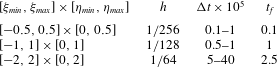
.
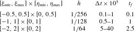
Table 2 lists parameters used in the computation: the mapped domain size, the mesh size
 $h$
, the time step
 ${\rm\Delta}t$
and the corresponding final time
 $t_{f}$
. The parameters
 $h$
,
 ${\rm\Delta}t$
and the domain size chosen are larger for longer final times. At a fixed final time,
 $h$
and the domain size are fixed and
 ${\rm\Delta}t$
is larger at larger wedge angles. For example, at
 $t_{f}=2.5$
and
 $h=1/64$
,
 ${\rm\Delta}t=0.5\times 10^{-5}$
for
 ${\it\beta}{\rm\pi}={\rm\pi}/3$
,
 ${\rm\Delta}t=2.5\times 10^{-5}$
for
 ${\it\beta}{\rm\pi}={\rm\pi}/2$
and
 ${\rm\Delta}t=4\times 10^{-4}$
for
 ${\it\beta}{\rm\pi}=2{\rm\pi}/3$
and
 $5{\rm\pi}/6$
.
2.4 Convergence study
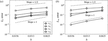
Figure 3 shows the convergence of the method. Errors in the vorticity
 ${\it\omega}$
, two components of the velocity
 $(u,v)$
and the streamfunction
 ${\it\psi}$
, over the whole domain, are measured in both
 $L_{2}$
and
 $L_{\infty }$
norms, (2.13). The time step
 ${\rm\Delta}t$
is chosen to be proportional to the mesh size
 $h$
. We use
 $h=1/16~({\rm\Delta}t=2\times 10^{-4})$
,
 $1/32~({\rm\Delta}t=1\times 10^{-4})$
,
 $1/64~({\rm\Delta}t=5\times 10^{-5})$
,
 $1/128~({\rm\Delta}t=2\times 10^{-5})$
in the computation. The solution at
 $h=1/128$
is assumed to be the exact solution:
 $$\begin{eqnarray}\displaystyle e_{{\it\omega}}^{h}=\frac{\Vert {\it\omega}^{h}-{\it\omega}^{1/128}\Vert }{\Vert {\it\omega}^{1/128}\Vert },\quad e_{u}^{h}=\frac{\Vert u^{h}-u^{1/128}\Vert }{\Vert u^{1/128}\Vert }, & & \displaystyle\end{eqnarray}$$
 $$\begin{eqnarray}\displaystyle e_{v}^{h}=\frac{\Vert v^{h}-v^{1/128}\Vert }{\Vert v^{1/128}\Vert },\quad e_{{\it\psi}}^{h}=\frac{\Vert {\it\psi}^{h}-{\it\psi}^{1/128}\Vert }{\Vert {\it\psi}^{1/128}\Vert }. & & \displaystyle\end{eqnarray}$$
Although a second-order approximation is applied in both space and time, as noted in § 2.2, it is seen that for the
 $L_{2}$
norm a half-order convergence is observed for all variables; for the
 $L_{\infty }$
norm, the half-order convergence is observed in
 ${\it\omega}$
and
 $v$
,
 $u$
is less than half order and
 ${\it\psi}$
is of first order. There could be four factors that affect the observed order of convergence: the splitting scheme for the inviscid and viscous parts of the vorticity (Strang Reference Strang1968), the usage of a semi-Lagrangian scheme for the vorticity convection (Falcone & Ferretti Reference Falcone and Ferretti1998), the large distortion of the mesh near the wedge tip in the physical domain and the singularity at the wedge tip.
Convergence study: (a)
 $L_{2}$
norm and (b)
 $L_{\infty }$
norm of errors in
 $e_{{\it\omega}}$
,
 $e_{\boldsymbol{u}}$
,
 $e_{\boldsymbol{v}}$
,
 $e_{{\it\psi}}$
, computed using (2.13), are plotted as functions of
 $h$
. Two lines of slope
 $1/2$
and 1 are plotted. Solutions are computed at
 $t=0.5$
and
 ${\it\beta}{\rm\pi}=2{\rm\pi}/3$
(
 $Re_{s}=329.87$
).

3 Results
This section presents the numerical results. Section 3.1 presents the solutions at a fixed wedge angle of
 $2{\rm\pi}/3$
. Section 3.2 shows the dependence of the solutions on varying wedge angles. Section 3.3 shows the vorticity and trajectory of the vortex centre, and the comparison with laboratory experiments and the self-similar theory.
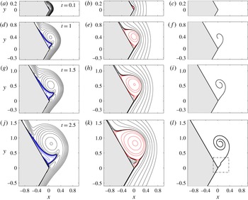
Evolution of vorticity
 ${\it\omega}$
(a,d,g,j), streamlines
 ${\it\psi}$
(b,e,h,k) and streaklines (c,f,i,l) at
 $t=0.1~(Re_{s}=125.59)$
,
 $1~(Re_{s}=500)$
,
 $1.5~(Re_{s}=637.71)$
and
 $2.5~(Re_{s}=866.43)$
. The wedge angle is
 ${\it\beta}{\rm\pi}=2{\rm\pi}/3$
. The vorticity contours are
 ${\it\omega}=\pm 2^{j},~j=-5,-4,\ldots ,9,10$
. The vorticity is positive in black and negative in blue. The streamlines are positive in red and negative in black. The outermost vorticity is positive and the outermost streamline is negative.

3.1 Vorticity, streamlines and streaklines at a fixed wedge angle
Figure 4 shows the evolution of the vorticity (a,d,g,j), the streamlines (b,e,h,k) and streaklines (c,f,i,l). The wedge angle is
 ${\it\beta}{\rm\pi}=2{\rm\pi}/3$
. Results at other wedge angles are qualitatively similar. In the plots of vorticity, it is seen that as the fluid moves from below to above the wedge, a boundary layer develops along the wall and thickens in time. The vorticity accumulates near the wedge tip on the leeward side, forming the starting vortex. Initially, all vorticity is positive, and the flow is in the Rayleigh stage (XN15). The Rayleigh stage is defined to be the time interval when the flow consists of only a positive vortical boundary layer. The vorticity is largest at the wedge tip. After some time, a negative vorticity region develops within the starting vortex at the wall, which is already visible at
 $t=0.1$
and 1. In the current study, the negative vorticity boundary layer at the wedge tip is denoted as the first vorticity region of alternate signs, and the time that it appears is denoted by
 $T_{1}$
.
 $T_{1}$
indicates the termination of the Rayleigh stage. We will study the dependence of
 $T_{1}$
on
 ${\it\beta}$
later on. The first vorticity region of alternate signs is observed at all times shown in figure 4.
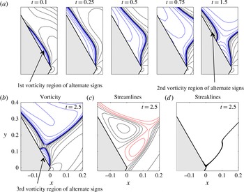
Enlargement of solutions near the wedge tip. (a) Contours of vorticity
 ${\it\omega}$
at
 $t\in [0.1,1.5]$
 $(Re_{s}\in [125.59,637.71])$
. Contours of (b) vorticity
 ${\it\omega}$
, (c) streamfunction
 ${\it\psi}$
and (d) streaklines at
 $t=2.5~(Re_{s}=866.43)$
. The wedge angle is
 ${\it\beta}{\rm\pi}=2{\rm\pi}/3$
. The vorticity is positive in black and negative in blue. The streamlines are positive in red and negative in black.

At
 $t=1$
, the vortex centre is present; it is the location of a local maximum vorticity. The starting vortex becomes better defined. The negative vorticity boundary layer grows thicker, further separating the starting vortex from the wedge. For
 $t\in [1,1.5]$
the shape of the starting vortex is similar but grows and is convected downstream. There is one primary recirculating region in the streamlines, associated with the negative vorticity region. The recirculation is enclosed by the zero-level streamline, starting at the wedge tip and ending somewhere on the wedge boundary. The flow inside the region is rotating counter-clockwise.
For
 $t\in [1.5,2.5]$
, the negative vorticity layer grows thicker and longer and is gradually entrained by the starting vortex. It is important to note that during this time a positive vorticity layer appears within the negative layer, and we denote this new layer as the second vorticity region of alternate signs; the time at which it appears is denoted by
 $T_{2}$
. In association with this new positive vorticity layer, a clockwise recirculating region forms in the streamlines, clearly seen on the edge at
 $t=1.5$
. At
 $t=2.5$
, another small counter-clockwise recirculating region forms at the wedge tip in the streamlines, indicating the appearance of the third vorticity region of alternate signs. In the end, hierarchical vorticity regions of alternate signs are created.
The streaklines at a given time are composed of all particles present in the fluid flow. The streaklines form a spiral; the particles that are released earlier travel closer to the vortex centre. The spiral grows and gets tighter near the vortex centre. Due to the presence of multiple recirculating regions in the streamlines, the streaklines near the wedge tip have a kink, as shown in the dashed box at
 $t=2.5$
.
Figure 5 is a closeup of the solution near the wedge tip. Figure 5(a) presents vorticity contours at a sequence of times, as indicated in the plots, which clearly show the formation of the first (
 $t=0.1$
) and second (
 $t=1.5$
) vorticity regions of alternate signs. At
 $t=0.1$
the vortex centre is not yet present. At
 $t=1.5$
, a ‘neck’ is formed between the second vorticity region of alternate signs and the outermost positive vorticity. The neck shrinks to zero as time increases, yielding the third vorticity region of alternate signs, as seen at
 $t=2.5$
in figure 5(b).
Figure 5(c) shows streamlines at time
 $t=2.5$
. Two rotation regions associated with the second and third vorticity regions of alternate signs are seen near the wedge tip. The size of the rotation region is proportional to the size of the corresponding vorticity region. A stagnation point in the streamlines is present on the wedge boundary near the tip. Figure 5(c) plots streaklines at time
 $t=2.5$
. The streaklines are tilted since they are influenced by the rotating flow in the second and third rotation regions.
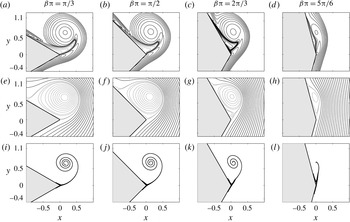
Contours of vorticity
 ${\it\omega}$
(a–d), streamlines
 ${\it\psi}$
(e–h) and streaklines (i–l) at
 $t=2$
for
 ${\it\beta}{\rm\pi}={\rm\pi}/3~(Re_{s}=452.86)$
,
 ${\rm\pi}/2~(Re_{s}=500)$
,
 $2{\rm\pi}/3~(Re_{s}=574.34)$
,
 $5{\rm\pi}/6~(Re_{s}=707.16)$
.

The appearance time of (a) the first vorticity region of alternate signs,
 $T_{1}$
versus
 ${\it\beta}$
, and (b) the second vorticity region of alternate signs,
 $T_{2}$
versus
 ${\it\beta}$
, on a linear scale.

3.2 Dependence on the wedge angle
Figure 6 compares the vorticity (a–d), streamlines (e–h) and streaklines (i–l) at
 $t=2$
at different wedge angles. The wedge angles are
 ${\rm\pi}/3$
,
 ${\rm\pi}/2$
,
 $2{\rm\pi}/3$
,
 $5{\rm\pi}/6$
from (a) to (l). The thick lines in the plots of vorticity consist of many small-scale vorticity contours which separate the positive and negative vorticity regions. At relatively small wedge angles of
 ${\it\beta}{\rm\pi}={\rm\pi}/3$
and
 ${\rm\pi}/2$
, the starting vortex is quite round and well defined, and the negative vorticity region is entrained further into the starting vortex. As the wedge angle increases, the starting vortex becomes elliptic. The elliptic shape of the starting vortex is also reported in Pullin (Reference Pullin1978) (figure 9 at
 $m=0$
). At
 ${\it\beta}{\rm\pi}=5{\rm\pi}/6$
, the driving flow is almost parallel to the wedge boundary and the starting vortex is still within the initial positive vortical boundary layer. At all wedge angles, the vortex centre is approximately the same height in the
 $y$
direction. The vorticity value of the centre is smaller at a larger wedge angle.
The streamlines in figure 6 show the presence of a large rotation region and the rotation centre. It is noted that the zero streamline leaving at the wedge tip is not tangential to the edge profile. The streamlines are denser at small wedge angles, indicating larger magnitudes in the velocity field. The second rotation region, which is associated with the second vorticity region of alternate signs, is only present at
 ${\it\beta}{\rm\pi}=2{\rm\pi}/3$
in these plots, suggesting a non-monotonic appearance time of
 $T_{2}$
as a function of the wedge angle. The third rotation region is absent without the second one. The shape of the streaklines is not quite sensitive to the initial locations of the fluid particles since all particles converge to a single spiral. The spiral is tighter at a smaller wedge angle. The heights of the vortex centre, the rotation centre and the centre of the spiral are almost the same, independent of the wedge angle.
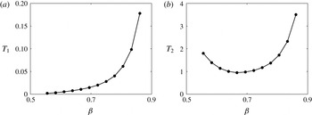
Figure 7 plots the appearance time of the first (
 $T_{1}$
) and second (
 $T_{2}$
) vorticity regions of alternate signs as a function of
 ${\it\beta}$
. Figure 7(a) plots
 $T_{1}$
at
 ${\it\beta}\in (0.5,0.9)$
. It is seen that
 $T_{1}$
is always positive, and increases as
 ${\it\beta}$
gets larger. Thus, the Rayleigh stage is present at the wedge angles considered here. Although the case of the zero wedge angle is not studied here, it is worth mentioning that XN15 found that the Rayleigh stage is absent for the impulsively started flow past a finite flat plate. At early times, the starting vortex is small compared to the finite plate length, and thus it is close to the case of the zero wedge angle. If the trend of
 $T_{1}$
in figure 7(a) holds,
 $T_{1}$
will go to zero as the wedge angle decreases to zero. On the other hand,
 $T_{1}$
increases rapidly for
 ${\it\beta}>0.7$
. It is expected that at
 ${\it\beta}=1$
, the case of a half-plane,
 $T_{1}$
is infinite. In the computation, it is found to be increasingly difficult to obtain
 $T_{1}$
at small wedge angles owing to the extremely small time steps.
Figure 7(b) shows
 $T_{2}$
as a function of
 ${\it\beta}$
. The value of
 $T_{2}$
is a few orders of magnitude bigger than that of
 $T_{1}$
. In the figure, it is seen that the value of
 $T_{2}$
first decreases and then increases as
 ${\it\beta}$
increases. Thus, one can immediately see that there exists a minimum of
 $T_{2}$
. The minimum takes place near
 ${\it\beta}=2/3$
. In the plot, there seems to be two vertical asymptotic lines, at
 ${\it\beta}=0$
and 1, respectively, at which the second vorticity region of alternate signs does not exist. In the computation, obtaining
 $T_{2}$
at a large wedge angle is difficult owing to quite a long final time.
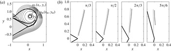
(a) Locations of the local vorticity maximum
 $(x_{m},y_{m})$
and rotation centre
 $(x_{c},y_{c})$
and their corresponding vorticities,
 ${\it\omega}_{m}$
and
 ${\it\omega}_{c}$
. (b) Trajectory of the vortex centre
 $(x_{m},y_{m})$
(solid line) and the rotation centre
 $(x_{c},y_{c})$
(dashed line) for
 $t\in [0,2.5]$
at
 ${\it\beta}{\rm\pi}={\rm\pi}/3$
,
 ${\rm\pi}/2$
,
 $2{\rm\pi}/3$
,
 $5{\rm\pi}/6$
.

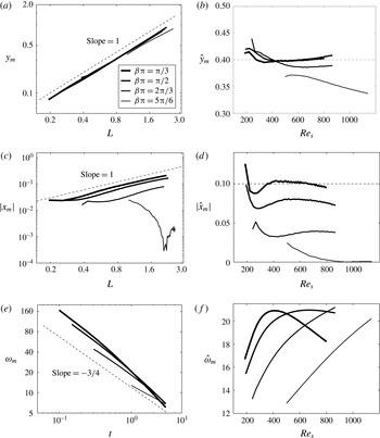
Coordinates and vorticity at the vortex centre are shown in two ways: (a,c,e) dimensional,
 $y_{m}$
versus
 $L$
,
 $|x_{m}|$
versus
 $L$
,
 ${\it\omega}_{m}$
versus
 $t$
; (b,d,f) non-dimensional,
 ${\hat{y}}_{m}$
versus
 $Re_{s}$
, (
 $|\hat{x}_{m}|$
versus
 $Re_{s}$
,
 $\hat{{\it\omega}}_{m}$
versus
 $Re_{s}$
. Here
 $L$
is from (2.4).

3.3 Scaling of vorticity and location of the vortex centre
Figure 8(a) plots the vorticity contours and two streamlines (thick curves), which helps to illustrate the locations of the vortex and rotation centres. The vortex centre has a local maximum of vorticity
 ${\it\omega}_{m}$
and is located at
 $(x_{m},y_{m})$
. The rotation centre has the local minimum of the streamfunction and is located at
 $(x_{c},y_{c})$
. We denote the vorticity at the rotation centre by
 ${\it\omega}_{c}$
. Figure 8(b) shows the trajectory of the vortex (solid line) and rotation (dashed line) centres at varying wedge angles for
 $t\in [0,2.5]$
. Both centres are formed at some distance from the wedge tip, farther away at a larger wedge angle. The rotation centre forms earlier in time than the vortex centre. Both centres are close to each other while travelling, with the vortex centre always on the right-hand side of the rotation centre. Their traces are along a straight line and both end at a height of
 $y\approx 0.8$
. It is noted that the
 $x$
component of the vortex centre decreases for
 ${\it\beta}{\rm\pi}=5{\rm\pi}/6$
while it increases for other wedge angles shown here.
Figure 9(a,c) show the coordinates of the vortex centre
 $(|x_{m}|,y_{m})$
as a function of
 $L$
on a logarithmic scale, where
 $L$
is computed using (2.4). It is seen that the value of
 $y_{m}$
scales linearly with respect to
 $L$
, independent of the wedge angle; this is consistent with the inviscid flow analysis of Pullin (Reference Pullin1978) (equation (31)). The curves of
 $|x_{m}|$
also follow the same linear scale with respect to
 $L$
. The value of
 $|x_{m}|$
is smaller at a larger wedge angle. The curve of
 $|x_{m}|$
at
 ${\it\beta}{\rm\pi}=5{\rm\pi}/6$
deviates from the linear scale since
 $x_{m}$
moves from a positive to a negative value, as indicated in figure 8(b). Figure 9(b,d) show the coordinates of the vortex centre in dimensionless variables,
 $(\hat{x}_{m},{\hat{y}}_{m})$
versus
 $Re_{s}$
. At
 ${\it\beta}{\rm\pi}={\rm\pi}/3$
,
 ${\hat{y}}_{m}$
seems to be a constant around 0.4 and
 $|\hat{x}_{m}|$
is around
 $0.1$
. These two constants are close to that reported in PP80 (0.318 and 0.060, p. 248, table 2).
Figure 9(e,f) show plots of
 ${\it\omega}_{m}$
versus
 $t$
and
 $\hat{{\it\omega}}_{m}$
versus
 $Re_{s}$
on a logarithmic scale, respectively. In figure 9(e), a reference dashed line of slope
 $-3/4$
is plotted. It is seen that
 ${\it\omega}_{m}$
scales as
 $t^{-3/4}$
and is independent of wedge angles during the time computed, which agrees with the observation in a finite plate in Xu & Nitsche (Reference Xu and Nitsche2014) (figure 8d). When
 $\hat{{\it\omega}}_{m}$
is plotted as a function of
 $Re_{s}$
, no apparent scaling is observed. The vorticity and trajectory of the rotation centre follow the same scaling since it is located very close to the vortex centre and therefore they are not shown here.
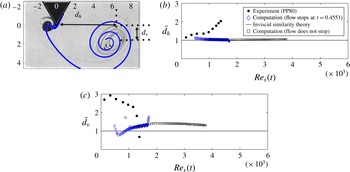
(a) Patterns of the fluid dyes in the experiment (black) and the streaklines in the computation (blue). Comparison of the horizontal (b)
 $\bar{d_{h}}$
and vertical (c)
 $\bar{d_{v}}$
displacements of the major spiral centre as a function of
 $Re_{s}$
, obtained from the experiment (PP80), computation (flow stops at
 $t=0.4551$
), and inviscid similarity theory. The computational result of figure 6 (flow does not stop) is also shown.
 $\bar{d_{h}}$
and
 $\bar{d_{v}}$
are scaled values (using equations (7a) and (8) in PP80) for the purpose of comparison. All experimental results are obtained from PP80.

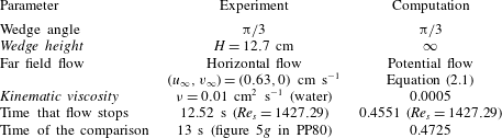
List of parameters in the experiment of Pullin & Perry (Reference Pullin and Perry1980) and the current numerical computation. The italic font highlights the differences between the experiment and computation.
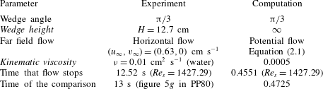
Pullin & Perry (Reference Pullin and Perry1980) experimentally visualized the starting vortex of viscous flow (water) past wedges using fluid dyes. In figure 10(a), the numerical result is compared with that of PP80 at the wedge angle
 ${\rm\pi}/3$
for an impulsively started flow. The reader is referred to PP80 (figure 1) for the experimental setup. In the experiment, the wedge edge had a finite length of
 ${\hat{H}}=12.7$
cm, attached to the ceiling of the water tank. The wedge had small holes where dyes were injected into the water. The driving flow moved horizontally from the left- to the right-hand side. The flow stopped at 12.52 s, and locations of dyes were shown at 13 s. In the computation, the wedge has an infinite length and the driving flow is the potential flow, (2.1). The fluid viscosity is chosen to be
 ${\it\nu}=0.0005$
. The flow in the computation stops at
 $t=0.4551$
and results are shown at
 $t=0.4725$
. Parameters in both the experiment and the computation are summarized in table 3.
Figure 10(a) shows the overlap of the fluid dyes in the experiment (black) and streaklines in the computation (blue). Two spirals in the streaklines are seen. One is the major spiral downstream and the other is relatively small and on the upstream side, close to the wedge tip. The small spiral is caused by the stopped incoming flow.
Consistency and discrepancy are seen in the comparison. The computation captures the size and a rough location of the major spiral in the downstream side and the presence of the small spiral in the upstream side. The discrepancy lies in the exact horizontal and vertical displacements of the major spiral centre from the wedge tip, denoted by
 $d_{h}$
and
 $d_{v}$
, respectively. The value of
 $d_{h}$
is larger and
 $d_{v}$
is smaller in the experiment. At this point it is natural to question what causes the differences in
 $d_{h}$
and
 $d_{v}$
. Two conjectures are proposed. The first conjecture is the difference in fluid viscosity. The other one is the difference in the far-field flow. We tend to rely on the second conjecture based on the following reasons. First, it is possible that the horizontal incoming flow in the experiments pushes the spiral centre further in the downstream direction, causing a larger value of
 $d_{h}$
. Second, the fluid flow is governed by the Navier–Stokes equations, and thus, it possesses memory in time. The potential driving flow in the computation moves around the wedge and has an overall larger vertical speed near the wedge tip compared with that in the experiment. Therefore, this might lead to a larger value in
 $d_{v}$
later on. Third, excellent agreement is seen between the experiment and computation when the numerical solution of viscous flow past a finite flat plate is compared with that of a
 $5^{\circ }$
wedge angle (XN15, figure 7). In that study, due to the symmetry of the finite plate about its centreline, one can consider the centreline as a slip wall; therefore, the far flow is the same as the horizontally incoming flow in the experiment.
Figure 10(b,c) compare the scaled values of the horizontal and vertical displacements,
 $\bar{d_{h}}$
and
 $\bar{d_{v}}$
, as a function of
 $Re_{s}(t)$
for results obtained from the experiment (PP80), computation (the flow stops at
 $t=0.4551$
) and the inviscid similarity theory. The computational result of figure 6 (the flow does not stop) is also shown. The formulas of
 $\bar{d_{h}}$
and
 $\bar{d_{v}}$
are given in PP80 ((7a) and (8)). The inviscid similarity theory indicates the limit of vanishing viscosity or a small time. It is observed that the computational solution of
 $\bar{d_{h}}$
follows the inviscid similarity theory prediction very well until the flow stops. The computational solution of
 $\bar{d_{v}}$
looks like a constant function in terms of
 $Re_{s}$
after a positive time, although that constant is larger than the inviscid prediction of 1. To conduct a more precise comparison with the experiment, one has to change the computational domain and make it the same as that in the experiment, in which there is a ceiling above the triangular wedge. However, this is a different problem and is beyond the scope of the current work.
4 Summary
This paper presents numerical simulations of impulsively started viscous flow past an infinite wedge of non-zero angles. We focus on the development of the starting vortex at the wedge tip, and the dependence of solutions on the wedge angles from early to moderate times. As far as we know, this is the first time that the structure and evolution of the viscous starting vortex behind wedges have been numerically investigated in great detail. The results can be summarized in two main aspects.
(1) A hierarchy of vorticity regions of alternate signs is observed at the wedge tip. The first vorticity region of alternate signs is marked by the appearance of the negative vortical boundary layer. The second region is marked by the appearance of a positive vortical boundary layer within the first one. The third region is the appearance of a small negative vorticity region next to the second one at the wedge tip. Each vorticity region of alternate signs is associated with a rotation region in the streamlines. The appearance times of the first and second vorticity regions are recorded. The appearance time of the first vorticity region of alternate signs increases monotonically with the wedge angle and appears to decrease/grow faster as the wedge angle reaches
 $0^{\circ }/180^{\circ }$
. The appearance time of the second vorticity region of alternate signs is large at either a small or large wedge angle. It has a minimum near the angle of
 $120^{\circ }$
.
(2) The vorticity and trajectory of the vortex centre are reported, and the results are compared with those from the laboratory experiment and the inviscid similarity theory. The vortex centre is at the local vorticity maximum in the starting vortex. The centre forms at a positive time, and it travels along a straight line. The location of the vortex centre is found to be consistent with the inviscid self-similar scaling. The vortex centre, rotation centre and spiral centre of the streaklines are close to each other. In comparison with the laboratory experiment, the aspects where we see agreement lie in the appearance of the major and secondary spirals on the downstream and upstream sides of the wedge. The locations of these two spirals approximately agree with those observed in the laboratory experiments. The aspects where we see discrepancy lie in the precise displacements of the major spiral centre from the wedge tip, and we think these differences are due to the different far-field flow in the computational setup.
Acknowledgements
Discussions with R. Krasny and M. Nitsche are gratefully acknowledged.