1. Introduction
In the study of different wall-bounded turbulent flows, the zero-pressure-gradient (ZPG) turbulent boundary layer is probably the most investigated, and perhaps the most reviewed. The ZPG boundary layer is also often considered as the baseline flow when examining various external influences such as roughness, streamwise pressure gradient, heat transfer, etc. However, significant challenges still exist in identifying the true statistical behaviour of a ZPG boundary layer, particularly at high Reynolds numbers (Marusic et al.
Reference Marusic, McKeon, Monkewitz, Nagib, Smits and Sreenivasan2010b
). One of the major challenges lies in unravelling under what conditions different experimental results can be credibly compared when assessing various scaling laws, such as outer-flow similarity. Comparisons of previous experimental data sets have shown significant discrepancies between different studies even though local experimental parameters are matched (Chauhan & Nagib Reference Chauhan and Nagib2008; Chauhan, Nagib & Monkewitz Reference Chauhan, Nagib and Monkewitz2009). Conventional wisdom suggests that provided the local Reynolds number is matched then comparisons can be made for assessing scaling behaviour, and this implicitly implies that no consideration is given to the evolution of the boundary layers. In the following we will show that such comparisons are not valid under certain conditions. Moreover, when anomalous behaviours have been noted in the literature, for example, such as the variation of Coles wake factor for
 $Re_{{\it\delta}^{\ast }}<5000$
(Coles Reference Coles1962), these have been described as a low-Reynolds-number effect. Again, in the following we will show that such trends are better described as an evolution effect resulting from the initial conditions set up by the trip and/or the initial inflow conditions.
Anomalous discrepancies between scaled data are not confined to experimental studies. Schlatter & Örlü (Reference Schlatter and Örlü2010) revealed large differences between direct numerical simulations (DNS) of the ZPG boundary layer for the shape factor
 $H={\it\delta}^{\ast }/{\it\theta}$
and skin-friction coefficient
 $C_{f}=2(U_{{\it\tau}}/U_{\infty })^{2}$
(
 ${\it\delta}^{\ast }$
is the displacement thickness,
 ${\it\theta}$
is the momentum thickness,
 $U_{{\it\tau}}$
is the skin-friction velocity and
 $U_{\infty }$
is the free-stream velocity). A likely cause for these disparities is the different evolution conditions for each boundary layer. A systematic DNS study by Schlatter & Örlü (Reference Schlatter and Örlü2012) re-simulated the canonical ZPG flow with varying inflow conditions and tripping effects. Schlatter & Örlü (Reference Schlatter and Örlü2012) suggest that the mean statistics and integral parameters agree well in the inner and outer layer for
 $Re_{{\it\theta}}>2000$
, provided transition is initiated inside the boundary layer at a low enough
 $Re_{{\it\theta}}$
(
 ${<}300$
, where
 $Re_{{\it\theta}}=U_{\infty }{\it\theta}/{\it\nu}$
is the Reynolds number based on free-stream velocity
 $U_{\infty }$
, momentum thickness
 ${\it\theta}$
and kinematic viscosity
 ${\it\nu}$
), and that under- or over-stimulation by the trip is avoided. They also concluded that the outer region of the boundary layer requires a longer inflow length to reach a fully turbulent state. Since direct numerical simulations are still at the lower end of the Reynolds number range where a scale separation starts to establish itself, currently the only way to investigate the influence of different tripping or inflow conditions in medium- to high-Reynolds-number boundary layers is through experiments. This is the approach used in the present study where we experimentally study the evolution of high-Reynolds-number ZPG turbulent boundary layers from different initial (tripping) conditions.
Although researchers have long recognised the importance of initial conditions in boundary layers, quantifiable and careful investigations of the role of the upstream conditions on the downstream flow have been sparsely reported. One of the first experiments performed in this area was by Erm & Joubert (Reference Erm and Joubert1991) who investigated the effect of various tripping conditions on turbulent boundary layers for Reynolds numbers between
 $715\leqslant Re_{{\it\theta}}\leqslant 2810$
. Erm & Joubert (Reference Erm and Joubert1991) proposed a technique for obtaining correctly stimulated turbulent boundary layers for a particular tripping device by changing the dimension of the trip iteratively until the measured Coles (Reference Coles1956) wake factor
 ${\it\Pi}$
agrees with the Coles (Reference Coles1962) curve of
 ${\it\Pi}$
versus
 $Re_{{\it\theta}}$
. Here
 $2{\it\Pi}/{\it\kappa}$
is the maximum deviation of the mean velocity profile from the log-law in the outer region. They also mentioned that the effectiveness of a given device in tripping a flow could be gauged to some extent by an examination of a plot of the associated
 $C_{f}$
versus
 $x$
relationship, where
 $x$
is the streamwise distance from the trip. Thus it was reasoned that if a given device was subjected to a series of free-stream velocities and plots of
 $C_{f}$
were produced for each velocity within the range, then an examination of the entire family of plots may indicate a velocity that will later, after further testing, be shown to be the velocity that leads to the Coles (Reference Coles1962) relationship being satisfied by the flow. This was validated by Erm & Joubert (Reference Erm and Joubert1991) with measurements. They made it very clear that each free-stream velocity would require a unique tripping device to properly stimulate the turbulent boundary layers. When the velocity is changed from the design value of the trip, the resulting deviation from the log-law is known to depart from the ideal form suggested by Coles (Reference Coles1962). The degree to which this deviation changes, and also how the mean flow parameters vary for a given Reynolds number with changes in flow velocity for different tripping devices, is yet to be investigated. Researchers have often presented measurements corresponding to fixed tripping configurations, but different free-stream velocities, based on the assumption that it is only the value of the local Reynolds number (e.g.
 $Re_{{\it\theta}}$
) that is important and not how the boundary layer was formed, i.e. no record of boundary layer evolution is necessary (see discussion in Hutchins Reference Hutchins2012). However, studies by Johansson & Castillo (Reference Johansson and Castillo2001), Castillo & Johansson (Reference Castillo and Johansson2002) and Castillo & Walker (Reference Castillo and Walker2002) showed that the mean velocity and Reynolds stress profiles collapse only in the outer part of the boundary layer when scaled in outer variables, provided the upstream conditions were fixed between the flows, and they concluded that the variation in Reynolds numbers in the boundary layer is mainly due to changes in the initial conditions.
1.1. Mean flow considerations
The classical self-similarity theory states that the mean velocity deficit profiles
 $U_{\infty }^{+}-U^{+}$
(
 $U_{\infty }$
is the free-stream velocity) of all ZPG boundary layers would be self-similar in the outer region when the Reynolds number is sufficiently high. The velocity deficit is generally expressed as a two-parameter relation utilising
 ${\it\eta}=z/{\it\delta}$
(here
 $z$
is the wall-normal position and
 ${\it\delta}$
is the boundary layer thickness) and the wake parameter
 ${\it\Pi}$
(Coles Reference Coles1956). The functional form of the velocity deficit profile is as follows:
 $$\begin{eqnarray}\displaystyle \frac{U_{\infty }-U}{U_{{\it\tau}}} & = & \displaystyle -\frac{1}{{\it\kappa}}\ln ({\it\eta})+\frac{2{\it\Pi}}{{\it\kappa}}[1-W({\it\eta},{\it\Pi})]\nonumber\\ \displaystyle & = & \displaystyle f({\it\eta},{\it\Pi}).\end{eqnarray}$$
Here
 $W$
is the wake profile such that
 $W(1,{\it\Pi})=1$
and it models the deviation of the mean velocity from the logarithmic law. Note that in this definition of
 ${\it\Pi}$
, the magnitude of
 ${\it\Pi}$
represents the deviation of
 $U^{+}$
from the log-law at
 $y={\it\delta}$
instead of the definition utilised by Coles (Reference Coles1956) where
 ${\it\Pi}$
is the maximum deviation from the log-law. The velocity deficit relation postulates that the self-similarity solution does not depend on the local Reynolds number: in other words, there is no ‘
 $x$
’ (streamwise distance) dependence when there is a sufficient boundary layer development length. The data surveyed over a wide range of Reynolds numbers by Coles (Reference Coles1962) showed that the wake parameter
 ${\it\Pi}$
becomes nominally constant for
 $Re_{{\it\theta}}\geqslant 8000$
. The scatter in the data at low Reynolds numbers not only led to questions about the validity of the experiments but also motivated new theories by Castillo & Johansson (Reference Castillo and Johansson2002), based on the ‘asymptotic invariance principle’ of George & Castillo (Reference George and Castillo1997). The principle asserts that in the limit as
 $Re\longrightarrow \infty$
, the boundary layer equations become independent of the friction Reynolds number (
 $Re_{{\it\tau}}={\it\delta}U_{{\it\tau}}/{\it\nu}$
), but the effect of the upstream conditions might be retained because the flow may always depend on them, even in the asymptotic limit. According to Castillo & Johansson (Reference Castillo and Johansson2002), the velocity deficit (1.1) assumes the following form:
 $$\begin{eqnarray}\displaystyle \frac{U_{\infty }-U}{U_{{\it\tau}}}=f({\it\eta},{\it\Pi},\ast ) & & \displaystyle\end{eqnarray}$$
(with a similar form also existing with
 $U_{\infty }$
as the velocity scale rather than
 $U_{{\it\tau}}$
), where ‘
 $\ast$
’ represents the upstream conditions and retains an influence over all Reynolds numbers, including the asymptotic high-
 $Re$
case.
Another possible explanation for the scatter in the data used by Coles (Reference Coles1962) is the strong dependence of
 ${\it\Pi}$
on the method by which it is extracted from the data and on how sensitive
 ${\it\Pi}$
and
 ${\it\delta}$
are to the particular curve fit used for the outer part of the mean velocity profile. This dependence was studied extensively by Monkewitz, Chauhan & Nagib (Reference Monkewitz, Chauhan and Nagib2008). In recent times, the progress in quantifying the deviation from the canonical state of the boundary layers has been encouraging; however, more data from different facilities are required before many of the questions can be answered satisfactorily. Considerable advances have been made by Monkewitz, Chauhan & Nagib (Reference Monkewitz, Chauhan and Nagib2007), Nagib, Chauhan & Monkewitz (Reference Nagib, Chauhan and Monkewitz2007) and Chauhan et al. (Reference Chauhan, Nagib and Monkewitz2009), who have proposed criteria to quantify when ZPG boundary layers are well behaved, i.e. they are representative of the canonical state. In the canonical state, evolution of mean flow parameters (such as
 ${\it\Pi}$
or
 $H$
) is governed only by the self-similarity of the mean defect velocity profile in the inertially dominated region. Their criteria are based on the assumption that the canonical asymptotic state is attained when the wake parameter
 ${\it\Pi}$
becomes invariant and/or the values of skin friction and shape factor are consistent with each other in the classical framework. Although it is satisfying that many high-quality experiments agree well with the asymptotic turbulent boundary layer theory and satisfy the criteria outlined by Chauhan et al. (Reference Chauhan, Nagib and Monkewitz2009), the prediction of development of boundary layers at low
 $Re$
is challenging due to the sensitivity of the boundary layer to influences immediately upstream.
This difficult problem of how the canonical asymptotic state evolves from an arbitrary initial condition (or a low-
 $Re$
state) was first tackled by Perry, Marusic & Li (Reference Perry, Marusic and Li1994) and Perry, Marusic & Jones (Reference Perry, Marusic and Jones2002) who computed the development of the ZPG boundary layer from a specified set of initial conditions using the momentum and continuity equations in simplified form. This involves the hypothesis that the total shear stress field is uniquely described by a two-parameter family. In addition, a relation between the mean flow and shear stress parameters is required to close the system of equations. Perry et al. (Reference Perry, Marusic and Li1994) and Perry et al. (Reference Perry, Marusic and Jones2002) have tentatively given a closure equation based on the data sets available to them at that time and showed that all the different evolution curves converge to a single bifurcation line, which can be regarded as equivalent to the asymptotic curves proposed by Nagib et al. (Reference Nagib, Chauhan and Monkewitz2007) to indicate when an evolving boundary layer becomes well behaved.
1.2. Paper outline
The main aim of the current work is to obtain high-quality data of boundary layers that develop spatially to high Reynolds number from different initial conditions, and to ascertain whether the boundary layers ever reach a well-defined or ‘fully developed’ state, allowing for meaningful comparisons of scaling behaviours between different experiments. This is done by considering three tripping devices for the same upstream conditions in a purpose-built wind tunnel with a long (27 m) working section. In the reminder of the paper a detailed description of the experiments is given, followed by comparisons of the mean flow, second-order statistics, including spectra, and high-order statistics of the streamwise velocity across the boundary layers at multiple streamwise stations. The second main aim of the study is to see where the classical approach such as the one developed by Perry et al. (Reference Perry, Marusic and Jones2002) can be used to compute the evolution of the flow in different developing states. This approach will be summarised in § 5 and computations and comparisons to experimental data will be presented in § 6.
2. Experimental setup
We here produce a set of detailed boundary layer measurements in a developing turbulent boundary layer at matched inlet conditions (achieved by matching the unit Reynolds number
 $U_{\infty }/{\it\nu}$
between experiments). Matched unit Reynolds number allows measurements made at the same
 $x$
location, yet acquired on different days, to have the same
 $Re_{x}$
even if the ambient temperature is different due to daily variations. In this case variations in friction Reynolds number,
 $Re_{{\it\tau}}=U_{{\it\tau}}{\it\delta}/{\it\nu}$
, are attained by measuring at increasing streamwise distances downstream of the tripped inlet to the working section (from
 $1.6<x<18~\text{m}$
) rather than by altering
 $U_{\infty }$
or
 ${\it\nu}$
. By keeping the unit Reynolds number constant, the flow conditioning, contraction, and trip can be considered unaltered for all measurements and hence the effect of streamwise development can be studied in isolation from the influence of inflow conditions. By contrast, in facilities where variation in
 $Re_{{\it\tau}}$
is attained by increasing the free-stream velocity (or reducing
 ${\it\nu}$
), one runs the risk of contaminating any genuine Reynolds number development with variations in the inflow conditions. For example, in such situations, even if the contraction, fan and flow conditioning perform similarly, and even if the pressure gradient is carefully adjusted, the magnitude of the tripping stimulation will increase with
 $U_{\infty }/{\it\nu}$
(see Erm & Joubert Reference Erm and Joubert1991).
2.1. Facility
The measurements were performed in the High-Reynolds-Number Boundary Layer Wind Tunnel in the Walter Basset Aerodynamics Laboratory at the University of Melbourne. This tunnel has a 27 m long working section, and is capable of generating free-stream velocities of up to
 $45~\text{m}~\text{s}^{-1}$
, although all measurements here are made at a nominal free-stream velocity of
 $20~\text{m}~\text{s}^{-1}$
. Careful upstream flow conditioning and a three-dimensional contraction, with a reduction area ratio of 6.2, yields a free-stream turbulence intensity (
 $\sqrt{\overline{u^{2}}}/U_{\infty }$
) of 0.05 % at the start of the working section, and in the range of 0.15–0.2 % at
 $x\approx 18~\text{m}$
(for a free-stream velocity range of
 $20<U_{\infty }<40~\text{m}~\text{s}^{-1}$
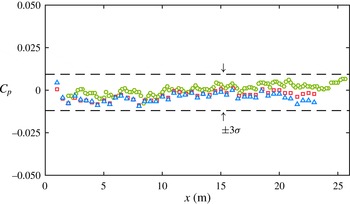
). A series of adjustable slots and panels on the ceiling of the working section enables precise control of the streamwise pressure gradient. For all experiments presented here the coefficient of pressure
 $C_{p}$
along the entire working section is constant to within
 $\pm 0.87\,\%$
(for all tripping configurations). Hence these experiments can be considered as concerning zero-pressure-gradient (ZPG) flows. Measurements are made in the turbulent boundary layer developing over the bottom wall of the working section. The 27 m long test surface permits the development of thick boundary layers. For example, with a free-stream velocity of
 $U_{\infty }\approx 20~\text{m}~\text{s}^{-1}$
, the boundary layer thickness varies from
 ${\it\delta}=0.06~\text{m}$
at
 $x=1.6~\text{m}$
from the tripped inlet, to
 ${\it\delta}=0.32~\text{m}$
at
 $x=18~\text{m}$
. The thick boundary layer enables us to attain good spatial resolution with a conventional hot-wire probe design.
Given the limited cross-sectional area of the working section (
 $1.89\times 0.92~\text{m}^{2}$
), compared to the very long length (27 m), careful attention was given to ensure that the boundary layers were nominally two-dimensional in the mean for the streamwise stations considered here. Nickels et al. (Reference Nickels, Marusic, Hafez and Chong2005) report that, based on the studies of Jones, Marusic & Perry (Reference Jones, Marusic and Perry1995) in a separate facility with adjustable side walls, the extra strain-rate effects due to finite working section width are negligible provided that the tunnel is wider than six boundary layer thicknesses
 $(6{\it\delta})$
, which is conservatively met to at least
 $x=18~\text{m}$
. Further tests are reported by Kulandaivelu (Reference Kulandaivelu2012) who conducted a spanwise survey of free-stream velocity at
 $U_{\infty }\approx 20~\text{m}~\text{s}^{-1}$
at
 $x=10.5~\text{m}$
over a spanwise distance of
 $0.8~\text{m}$
either side of the tunnel centreline, and found the variation to be less than
 $\pm$
0.35 % with no distinguishable slope in the velocity variation across the width of the boundary layer (corresponding to over
 ${\rm\Delta}y\approx 8{\it\delta}$
at this streamwise station). The wind tunnel also contains corner fillets throughout the facility. Comparisons of turbulence statistics at
 $x=21~\text{m}$
, with and without corner fillets in the working section, revealed no discernible differences, providing further confidence that the boundary layers at all streamwise locations reported here are nominally two-dimensional in the mean.
2.2. Hot-wire anemometery
All measurements were made using slightly modified Dantec 55P15 single-normal boundary layer type probes with prong tip spacing of 1.5 mm. Platinum–wollaston wires are soldered to the prong tips and etched to produce a
 $2.5~{\rm\mu}\text{m}$
diameter platinum sensing element of length
 $l\approx 0.54~\text{mm}$
, resulting in a length to diameter ratio,
 $l/d\approx 215$
(see Ligrani & Bradshaw Reference Ligrani and Bradshaw1987; Hutchins et al.
Reference Hutchins, Nickels, Marusic and Chong2009). These sensors are driven in constant-temperature mode using in-house-designed Melbourne University Constant-Temperature Anemometers (MUCTA) with an overheat ratio of 1.8. The system response was verified using a square-wave electronic test to ensure a second-order response and demonstrating a
 $-3$
dB drop-off (based on the definition of Freymuth Reference Freymuth1967) at 18 to 32 kHz for mean velocities in the range
 $0<U<20~\text{m}~\text{s}^{-1}$
. Hutchins et al. (Reference Hutchins, Monty, Hultmark and Smits2015) have recently shown that the temporal performance of all optimally tuned (under-damped) CTAs may start to diminish at frequencies lower than the
 $-3$
dB drop-off (at approximately 7–10 kHz). In this case, however, where high Reynolds numbers are attained with relatively low speeds and large development lengths, the frequency content of the turbulent boundary layer is relatively low. Hutchins et al. (Reference Hutchins, Nickels, Marusic and Chong2009) have shown that there is negligible energy content for
 $f^{+}>1/3$
(where
 $f^{+}=f{\it\nu}/U_{{\it\tau}}^{2}$
and
 $f$
is the frequency of turbulent fluctuations in Hz), which corresponds to frequencies of approximately 10 kHz for these measurements. Hutchins et al. (Reference Hutchins, Monty, Hultmark and Smits2015) estimate the error due to frequency response in the peak variance of
 $u$
at
 $zU_{{\it\tau}}/{\it\nu}=15$
to be less than 0.5 % for most anemometers provided that
 $U_{{\it\tau}}^{2}/{\it\nu}<0.3\times 10^{-5}~\text{s}^{-1}$
. For the present experiments,
 $U_{{\it\tau}}^{2}/{\it\nu}\approx 0.35\times 10^{-5}~\text{s}^{-1}$
.
In terms of spatial resolution, since the unit Reynolds number is everywhere matched, the only variation in the viscous-scaled wire length
 $l^{+}$
occurs due to the weak variation in
 $U_{{\it\tau}}$
along the development length of the facility. At
 $x=1.6$
, the 0.54 mm long sensing element yields
 $l^{+}=25.6$
, falling to 22.3 at
 $x=18~\text{m}$
. Hence, the probes can be considered to be nominally matched in terms of viscous length to within
 $24\pm 2$
.
2.3. Data acquisition
The hot-wire signals were sampled at 65 kHz, using a Data Translations DT9836 analogue–digital converter. This equates to a viscous-scaled sample interval of
 $0.41<{\rm\Delta}t^{+}<0.53$
for the range of experiments (
 ${\rm\Delta}t=1/f_{s}$
is the time between samples, where
 $f_{s}$
is sampling frequency). This exceeds the minimum timescale for energetic turbulent fluctuations (which is estimated at
 $t^{+}\approx 3$
, Hutchins et al.
Reference Hutchins, Nickels, Marusic and Chong2009), and thus the Nyquist criterion is met and aliasing is unlikely to be an issue. To be sure, the fluctuating signals are filtered at 25 kHz using a low-pass analogue filter. The total sampling time in seconds at each wall-normal position (
 $z$
) is given by
 $T$
. This is normalised in outer variables to give boundary layer turnover times
 $TU_{\infty }/{\it\delta}$
. For converged statistics, these numbers need to be large, since the largest structures in turbulent boundary layers can exceed
 $20{\it\delta}$
(e.g. Kim & Adrian Reference Kim and Adrian1999; Hutchins, Ganapathisubramani & Marusic Reference Hutchins, Ganapathisubramani and Marusic2004; Guala, Hommema & Adrian Reference Guala, Hommema and Adrian2006; Hutchins & Marusic Reference Hutchins and Marusic2007b
) and we would typically require several hundreds of these events to flow past the hot-wire sensor before we could expect converged statistics. In this study, the total sampling time was set in such a way that the boundary layer turnover time was in the range of 12 000–26 000 for all Reynolds numbers tested.
2.4. Calibration
The wires were calibrated statically against a Pitot-static tube located at the centreline of the tunnel in the undisturbed free stream. Calibrations are performed before and after each boundary layer traverse (referred to here as pre- and post-calibrations). To account for calibration drift during the experiments, the probe is periodically traversed to the free stream within the boundary layer profile measurement. At this free-stream excursion, the mean voltage measured by the hot wire and the mean velocity measured by the Pitot-static tube provides an additional re-calibration point at various intervals during the boundary layer traverse. Effectively, this means that for every six measurements during the boundary layer traverse (which consisted of between 33 and 50 logarithmically spaced measurement stations), the probe is re-calibrated. This procedure leads to a considerable reduction in the scatter between repeat experiments and is described in detail by Kulandaivelu (Reference Kulandaivelu2012) and Talluru et al. (Reference Talluru, Kulandaivelu, Hutchins and Marusic2014).
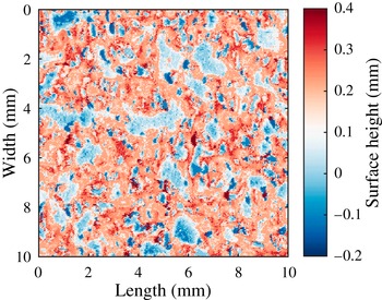
Contour plot depicting a scanned section (10 mm
 $\times$
10 mm) of the SP40 tripping configuration (P40 grit sandpaper). The colour bar on the right-hand side shows the distance from the mean plane (mm). Detailed specifications are given in table 1.

2.5. Tripping devices
Three flow cases were studied, corresponding to three different tripping configurations. All trips were introduced at the inlet to the working section (at
 $x=0$
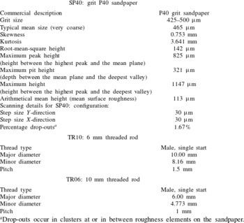
for the axis system used in this paper). The initial set of measurements was performed with the ‘standard’ tripping configuration, which consisted of a strip of P40 grit sandpaper, of length 154 mm in the streamwise direction. This trip was originally selected for this facility to obtain nominal shape factor values for ZPG turbulent boundary layers according to the recommendations of Erm & Joubert (Reference Erm and Joubert1991). The next two tripping configurations were deliberately chosen to over-stimulate the boundary layer to study the effect of the trip on the evolution of mean flow parameters. In these configurations, 6 and 10 mm diameter threaded rods were added at
 $x=0$
. We refer to the sandpaper and threaded rod configurations throughout as SP40, TR06 and TR10. Specifications of each trip configuration are given in table 1 and a representative scan of the sandpaper topography is shown in figure 1. To obtain consistent sets of measurements throughout the course of the investigation, reference conditions were fixed so that they corresponded to a given reference Reynolds number per metre. Here the nominal reference free-stream velocity for all three cases was
 $20~\text{m}~\text{s}^{-1}$
, resulting in a reference Reynolds number per metre of
 $U_{\infty }/{\it\nu}=1.295\times 10^{6}~\text{m}^{-1}$
.
Specifications of the tripping configurations.

a Drop-outs occur in clusters at or in between roughness elements on the sandpaper.
2.6. Streamwise pressure gradient
Since the pressure gradient plays an important role in the evolution of turbulent boundary layers, it is necessary to document the static pressure distribution along the length of the tunnel floor for all tripping configurations. The coefficient of pressure,
 $C_{p}$
, along the working section is constant to within
 $\pm 0.87\,\%$
for SP40 configuration as indicated in figure 2. Necessary adjustments are made to the roof of the working section to achieve the desired zero pressure gradient. The static pressure distribution for TR10 and TR06 configurations are also in figure 2. Since the streamwise pressure distributions for all the tripping configurations exhibit negligible acceleration or deceleration of the flow, they can all be considered in a state of constant pressure.
Streamwise pressure gradient for a reference free-stream velocity
 $U_{\infty }=20~\text{m}~\text{s}^{-1}$
. The downstream distance from the trip is given in the abscissa, whereas the ordinate denotes the variation of the coefficient of pressure in the
 $x$
direction. ○, SP40; ♢, TR10; ▫, TR06. The static pressure was measured at 20 cm and 50 cm intervals for the length of the tunnel floor for the SP40 configuration and TR10 & TR06 configurations, respectively.

3. Canonical reference case (SP40)
Table 2 collates the key experimental parameters for the set of matched-unit-Reynolds-number experiments conducted on the turbulent boundary layer developing downstream of the standard P40 sandpaper trip. This represents what has previously been considered to be the canonical case ZPG turbulent boundary layer in the large Melbourne wind tunnel. The SP40 will be the reference measurement to compare with the over-stimulated cases in § 4. For all three configurations, the measured mean velocity
 $U$
is fitted to the composite profile of Chauhan et al. (Reference Chauhan, Nagib and Monkewitz2009) to determine the local parameters
 $U_{{\it\tau}}$
,
 ${\it\delta}$
and
 ${\it\Pi}$
. The log-law constants in the composite profile are
 ${\it\kappa}=0.384$
and
 $B=4.17$
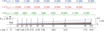
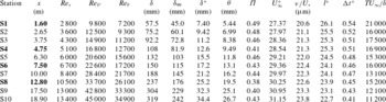
. Reynolds number and integral parameters listed in table 2, and table 3 in § 4, are calculated using the fitted composite profile. Figure 3 shows a schematic representation of the working section, showing the streamwise measurement stations, trip location and boundary layer development. Boundary layer traverses were conducted at 10 streamwise locations (S1 to S10) downstream of the trip, at
 $x=1.60$
, 2.65, 3.75, 4.75, 6.3, 7.5, 10, 12.8, 17.5 and 18.9 m. The local friction Reynolds number (
 $Re_{{\it\tau}}$
) together with local displacement-thickness Reynolds number (
 $Re_{{\it\delta}^{\ast }}={\it\delta}^{\ast }U_{\infty }/{\it\nu}$
) and the local momentum-thickness Reynolds number (
 $Re_{{\it\theta}}$
) for the SP40 trip case are also indicated for each measurement station.
Schematic of the boundary layer development along the test section of the wind tunnel. S1 to S10 indicate measurement stations.

Experimental parameters for the 10 profiles of the SP40 configuration. Bold notation for streamwise distance
 $x$
indicates that it is a common measurement station with the TR06 and TR10 configurations in table 3.

Over these 10 measurement stations the boundary layer develops from a friction Reynolds number of
 $Re_{{\it\tau}}\approx 2700{-}13\,000$
. Such Reynolds numbers are significant in terms of real-life engineering systems. For example, at the furthest downstream measurement station, the friction Reynolds number is equivalent to that obtained 6.7 m downstream of the nose (at the first passenger window) on a Gulfstream G550 cruising at an altitude of 14 500 m and at Mach 0.86 (Palumbo Reference Palumbo2013). Figure 3 also shows the mean velocity profiles developing downstream of the P40 trip, plotted as
 $U/U_{\infty }$
versus
 $z$
, clearly demonstrating the growth in boundary layer thickness and fullness of the profile as
 $x$
increases. The dash-dotted line on this plot shows the growth in boundary layer thickness
 ${\it\delta}$
, which exhibits a seemingly linear behaviour with
 $x$
for this particular configuration. In this study the boundary layer thickness
 ${\it\delta}$
, the skin-friction velocity
 $U_{{\it\tau}}$
and the wake parameter
 ${\it\Pi}$
are determined using the composite velocity profile fit of Chauhan et al. (Reference Chauhan, Nagib and Monkewitz2009).
Figure 3 also shows the contour of the outer limit of the overlap region, typically considered to be
 $0.15{\it\delta}$
, as the dashed line. This is helpful in realising that in the actual measurements the overlap region spans a small fraction of the total boundary layer thickness. If the Reynolds number is increased by increasing the free-stream velocity then the outer limit of the log-law indicated in figure 3 will move further towards the wall, making the task of accurately resolving velocities in this region even more challenging.
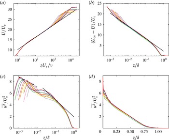
(a) Inner-normalised mean velocity profiles corresponding to the 10 streamwise hot-wire measurements acquired for the SP40 configuration. Straight line indicates the log-law
 $U^{+}=1/0.384\ln (z^{+})+4.17$
, (b) mean velocity defect profiles. Straight line corresponds to
 $(U_{\infty }-U)^{+}=2.3-1/0.384\ln (z/{\it\delta})$
, (c) streamwise Reynolds normal stress
 $\overline{u^{2}}^{+}$
versus
 $z/{\it\delta}$
on log-scale. Filled symbols indicate the peak magnitude of
 $\overline{u^{2}}$
for each profile. The solid straight line corresponds to (3.1), and the dashed line is from (3.2), where the slope is as reported by Lee & Moser (Reference Lee and Moser2015), (d)
 $\overline{u^{2}}^{+}$
versus
 $z/{\it\delta}$
on linear axes.

Figure 4(a) shows the measured mean velocity profiles normalised in wall units. As mentioned above, the friction velocity
 $U_{{\it\tau}}$
is determined by fitting the data to the composite velocity profile of Chauhan et al. (Reference Chauhan, Nagib and Monkewitz2009) (with log-law constants
 ${\it\kappa}=0.384$
and
 $B=4.17$
), and hence the collapse of the data on to the logarithmic law, marked by the straight line in figure 4(a), is forced. However, figure 4(a) demonstrates that the mean velocity profiles have a pronounced region of logarithmic behaviour at all measurement stations. This is reinforced by the velocity defect plots shown in figure 4(b) where a reasonable collapse to the logarithmic law is also seen for all profiles.
Figure 4(c) shows the profiles for
 $\overline{u^{2}}$
normalised by
 $U_{{\it\tau}}^{2}$
against the outer-scaled wall-normal height
 $z/{\it\delta}$
that correspond to the 10 mean velocity profiles in figure 4(a) for the SP40 configuration. A good outer-scaling collapse is observed for nominally
 $z/{\it\delta}\geqslant 0.1$
. For the logarithmic region the
 $\overline{u^{2}}/U_{{\it\tau}}^{2}$
profiles appear to reasonably well follow the logarithmic behaviour
 $$\begin{eqnarray}\frac{\overline{u^{2}}}{U_{{\it\tau}}^{2}}=B_{1}-A_{1}\ln (z/{\it\delta}),\end{eqnarray}$$
as most recently discussed in Marusic et al. (Reference Marusic, Monty, Hultmark and Smits2013), with
 $A_{1}=1.26$
and
 $B_{1}=1.95$
. At higher Reynolds numbers the region over which (3.1) is valid increases (see figure 2 of Marusic et al.
Reference Marusic, Monty, Hultmark and Smits2013). As expected, in the near-wall region, outer scaling does not apply; however, with inner scaling (
 $z^{+}=zU_{{\it\tau}}/{\it\nu}$
) a Reynolds-number independent scaling for
 $\overline{u^{2}}/U_{{\it\tau}}^{2}$
is not achieved either. The peak of
 $\overline{u^{2}}/U_{{\it\tau}}^{2}$
is seen to clearly increase with increasing Reynolds number, consistent with what has been extensively reported in the literature, e.g. DeGraff & Eaton (Reference DeGraff and Eaton2000), Hutchins et al. (Reference Hutchins, Nickels, Marusic and Chong2009), Klewicki (Reference Klewicki2010), Marusic et al. (Reference Marusic, McKeon, Monkewitz, Nagib, Smits and Sreenivasan2010b
) and others. The location at which the peak occurs (
 $z_{max}$
) is considered to be fixed in the inner scaling, i.e.
 $z_{max}^{+}\approx 15$
for ZPG turbulent boundary layers, and hence
 $z_{max}/{\it\delta}$
moves to the left with increasing Reynolds number in figure 4(c). The peaks are indicated by the filled symbols. A least-squares-error curve fit of these 10 points to the relation
 $$\begin{eqnarray}\frac{\overline{u^{2}}_{max}}{U_{{\it\tau}}^{2}}=B_{2}-A_{2}\ln (z_{max}/{\it\delta})\end{eqnarray}$$
returns
 $A_{2}=0.7$
and
 $B_{2}=3.9$
, which is generally consistent with results reported by Inoue et al. (Reference Inoue, Mathis, Marusic and Pullin2012). Recently, Lee & Moser (Reference Lee and Moser2015) surveyed DNS channel flow data up to
 $Re_{{\it\tau}}=5200$
, and reported a best fit of the peak variance results to be
 $\overline{u^{2}}_{max}^{+}=3.66+0.642\ln (Re_{{\it\tau}})$
. The dashed line in figure 4(c) corresponds to (3.2) using the same slope as that of Lee & Moser (Reference Lee and Moser2015) (
 $A_{2}=0.642$
;
 $B_{2}=4.26$
), and it is seen to be in good agreement to within the experimental uncertainty of the measurements. It is noted that such a comparison of
 $A_{2}$
between DNS and the experiments here is only possible because we have maintained a fixed sensor length in wall units for all measurements (
 $l^{+}\approx 24$
). While the additive constant (
 $B_{2}$
) is not expected to match the DNS results, as the limited sensor length will involve some attenuation of
 $\overline{u^{2}}^{+}$
, the slope of (3.2) should not change with the reasonable assumption that the energy-contributing scales not resolved fully with a sensor of
 $l^{+}\approx 24$
scale with viscous wall units (Chin et al.
Reference Chin, Hutchins, Ooi and Marusic2009; Marusic, Mathis & Hutchins Reference Marusic, Mathis and Hutchins2010a
). Similarly, figure 4(d) shows the profiles for
 $\overline{u^{2}}$
against the wall-normal distance
 $z/{\it\delta}$
in linear scale. The outer similarity of normalised
 $\overline{u^{2}}(z)$
with
 $U_{{\it\tau}}$
and
 ${\it\delta}$
as velocity and length scales, respectively, is evident in this figure.
The results presented so far for the SP40 configuration will suffice to establish that these measurements represent the canonical zero-pressure-gradient turbulent boundary layer and are in very good agreement with the known scaling behaviour for
 $U$
and
 $\overline{u^{2}}$
. Other results for this configuration will be discussed in comparison with the TR06 and TR10 configurations.
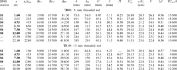
Experimental parameters for eight and six profiles of the TR06 and TR10 configurations respectively. Bold notation for streamwise distance
 $x$
indicates that it is a common measurement station for all three tripping configurations.
 $d_{trip}$
corresponds to trip height.

4. The over-stimulated boundary layers – TR06 and TR10
In this section we examine the evolution of the boundary layers that are ‘over-tripped’ by adding 6 and 10 mm threaded rods to the sandpaper trip (TR06 and TR10 configurations respectively). The mean flow parameters for TR06 and TR10 configurations are listed in table 3. Measurements were performed at eight and six streamwise locations for the 6 and 10 mm threaded rod trips, respectively. The streamwise locations that are common to all three trip configurations (SP40, TR06 and TR10) are indicated by bold notation in the table. The boundary layer thickness
 ${\it\delta}$
, skin-friction velocity
 $U_{{\it\tau}}$
and the wake parameter
 ${\it\Pi}$
are determined using the composite velocity profile fit of Chauhan et al. (Reference Chauhan, Nagib and Monkewitz2009) as was done for the SP40 configuration. The perturbations introduced by the threaded rods are more abrupt than those emerging from the sandpaper, resulting in larger boundary layer thicknesses at a given
 $x$
. Since the incoming unit Reynolds number (
 $U_{\infty }/{\it\nu}$
) is the same for all three configurations,
 $Re_{x}$
is the same at a particular streamwise location. However the changes in
 ${\it\delta}$
(and integral thicknesses) result in the TR06 and TR10 configurations having a much higher friction Reynolds number than SP40 for
 $x\leqslant 10~\text{m}$
. Hence these two configurations represent over-stimulated boundary layers.
4.1. Mean velocity
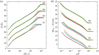
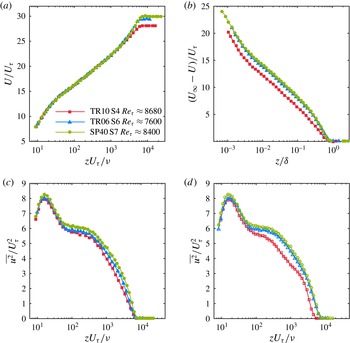
Figure 5(a) shows the mean velocity profiles using inner normalisation at four different streamwise locations. Profile measurements for all three trips are available at these four locations and hence a direct comparison can be made. The agreement of the
 $U^{+}$
versus
 $z^{+}$
profiles for all three configurations in the logarithmic region and below is expected since the inner normalisation utilises
 $U_{{\it\tau}}$
determined from a composite profile fit. However at Station S1 significant differences are observed in the outer wake region. Noticeably,
 $U^{+}$
in the wake region for SP40 is higher than TR06, which in turn is higher than TR10. Hence TR06 and TR10 configurations have a smaller value of
 ${\it\Pi}$
than SP40 at Station S1. This systematic deviation persists further downstream at Stations S4 and S6, although the severity of the deviation is observed to lessen with increasing streetwise distance. At the last common station of Station S8 we observe that all three profiles are in good agreement with each other in terms of wake strength although the TR10 case has a greater boundary layer thickness than TR06 and SP40. Hence we can conclude that the threaded rods as transition triggers over-stimulated the boundary layer such that the scaling of the mean velocity in the wake region is altered. We emphasise here that the streamwise length required for the over-stimulated boundary layers to recover to a canonical state is specific to the flows considered here. A larger trip than TR10 will invariably require a longer recovery length.
Comparison of mean velocity profiles for the three trips at four streamwise locations. ●, SP40; ▴, TR06; ▪, TR10. Note the vertical shift in profiles.

In the inner region, all the profiles in figure 5(a) are seen to agree following the law of the wall. However, it should not be inferred that differences in the three cases (SP40, TR6 and TR10) are confined only to the outer region. The influence of a different trip is felt throughout the boundary layer and this is readily seen if one considers the defect profiles, as shown in figure 5(b). We find that at Station S1, the defect throughout the layer is highest for SP40 while it is relatively the lowest for the TR10 case. This implies that the profiles for TR06 and TR10 trips are ‘fuller’ and the mean velocities in the outer region are closer to the free stream in these cases. The systematic deviations observed in the defect profiles decrease with increasing
 $x$
and eventually the outer similarity is regained by Station S8. It is only due to the change in corresponding
 $U_{{\it\tau}}$
that we see collapse in
 $U^{+}$
versus
 $z^{+}$
in the inner region. Outer scaling does not exist at low
 $x$
because we have perturbed the boundary layer in the outer region.
Based on figure 5(a,b) we can conclude that an obvious effect of different trips is to modify the mean flow immediately downstream of the trip. The mean boundary layer in the three configurations becomes identical further downstream, as marked by the collapse of inner- and outer-scaled velocity profiles. The rate at which the over-stimulated boundary layers return to the canonical state depends on the incoming free-stream velocity and type of trip. In this study the TR06 configuration approaches the canonical state faster than the TR10. This point is elaborated on later.
4.2. Streamwise Reynolds normal stress
The changes to the streamwise Reynolds normal stress
 $\overline{u^{2}}$
are examined in figure 6. The widely accepted inner scaling by
 $U_{{\it\tau}}^{2}$
for
 $\overline{u^{2}}$
is utilised here and again we find that the three profiles deviate considerably from each other at Station S1 downstream of the trip. The increased
 $Re_{{\it\tau}}$
values for the TR06 and TR10 cases are evident towards the edge of the layer where
 $\overline{u^{2}}\rightarrow 0$
. In the logarithmic region, unlike
 $U^{+}$
versus
 $z^{+}$
in figure 5(a) where a collapse of profiles was observed, the
 $\overline{u^{2}}/U_{{\it\tau}}^{2}$
profiles are seen to diverge. Close to the wall (in the vicinity of
 $z^{+}=15$
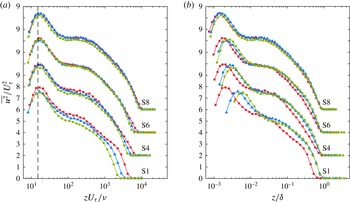
) the observed differences are relatively small, but the peak value for TR10 at Station S1 is distinctly higher. This indicates that the large-scale perturbations introduced in the outer part by the threaded rod change the structure of turbulence in the bulk of the layer, and the influence of these large scales appears to be felt well into the near-wall region during the initial development of the highly over-stimulated boundary layers (this will be shown more clearly when comparing spectra in § 4.4). Further downstream at Station S4 the deviation of profiles from each other is smaller than that seen at Station S1 but noticeably larger in the wake region. The profiles agree well with each other in the near-wall and logarithmic region at Station S6 but small differences still exist near the edge of the layer. It is clear that differences in the turbulence structure persist longer in the outer region, similarly to the differences in the mean velocity in figure 5(a). Finally, by Station S8 all profiles show an agreeable collapse and the three boundary layers appear to be similar. Thus we find that for the same
 $Re_{x}$
(by keeping
 $x$
the same) the three trip configurations result in three different states of the boundary layer with respect to the structure of their mean velocity and streamwise normal Reynolds stress. Reynolds number similarity clearly does not hold in the downstream region of the trip. Only after a certain development length do the over-stimulated flows ‘relax’ to a state that can be classically considered as canonical. In our study, for the chosen trip configurations this development length is at least 12.8 m, corresponding to
 $Re_{x}=1.7\times 10^{7}$
and up to
 $O(2000)$
trip-height lengths.
Comparison of
 $\overline{u^{2}}$
for the three trips at four streamwise locations. ●, SP40; ▴, TR06; ▪, TR10. Note the vertical shift in profiles by 2 units.


4.3. Comparisons at matched local Reynolds number
Above, comparisons were shown at matched
 $Re_{x}$
, and it is worthwhile to also consider the similarities and differences at matched local Reynolds numbers. Figure 7 shows comparisons of the above statistics at a nominally matched
 $Re_{{\it\tau}}\approx 8000$
. For the mean flow, the profiles of SP40 at
 $x=10~\text{m}$
, and TR06 at
 $x=7.5~\text{m}$
are seen to match very well, although small differences remain for
 $\overline{u^{2}}^{+}$
suggesting that remnants of the initial tripping conditions persist. In the case of the highly over-tripped TR10 flow at
 $x=4.75~\text{m}$
both the mean velocity and the normal Reynolds stresses are seen to be notably different to the SP40 case, with a greatly reduced wake region for the mean flow, and a
 $\overline{u^{2}}^{+}$
profile that has a slightly smaller peak value at
 $z^{+}\approx 15$
and a less full outer region, which at face value would be interpreted as a breakdown of Townsend’s outer-layer similarity hypothesis. Before proceeding further it is noted the comparisons in figure 7(a–c) are not for perfectly matched values of
 $Re_{{\it\tau}}$
. Therefore, the results of a check are shown in figure 7(d) where the streamwise stations of the three flows on either side of
 $Re_{{\it\tau}}=8000$
were interpolated to obtain an estimated profile at
 $Re_{{\it\tau}}=8000$
. For example, the profile for TR10 in figure 7(d) was obtained by linear-interpolating the
 $\overline{u^{2}}^{+}$
profiles at matched values of
 $z/{\it\delta}$
for profiles at
 $x=1.6~\text{m}$
,
 $Re_{{\it\tau}}=5850$
and
 $x=4.75~\text{m}$
,
 $Re_{{\it\tau}}=8680$
, weighted on
 $Re_{{\it\tau}}$
. The trends in figures 7(c) and 7(d) are seen to agree and therefore we conclude that the differences in the
 $Re_{{\it\tau}}$
values for the profiles in figure 7(a–c) is not the cause of the different trends noted. Rather, the lack of agreement between figures 7(c) and 7(d) is clearly due to the under-developed states of the over-stimulated boundary layers. This serves as a stark warning when comparing different experimental results based on matched
 $Re_{{\it\tau}}$
without consideration of the tripping conditions and evolution of the boundary layers. A further complication when considering Reynolds-number similarity in comparisons of different experimental results is what local Reynolds number to consider. In the wall turbulence literature
 $Re_{{\it\theta}}$
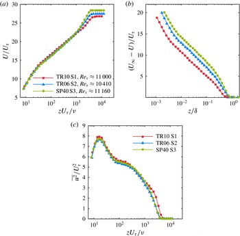
is commonly used and figure 8 shows the same comparisons as in figure 7 but here for nominally matched profiles at
 $Re_{{\it\theta}}\approx 10\,400$
. Curiously, the results show that while the
 $\overline{u^{2}}^{+}$
profiles appear to be in nominal agreement, apart from a departure of the TR10 results in the outermost region of the flow, the mean flow profiles show distinct differences. These results further highlight the pitfalls of comparing statistics at matched Reynolds numbers if the boundary layers have not recovered from inappropriately chosen trips. In these cases it is clear that there is no one-to-one correspondence between
 $Re_{{\it\tau}}$
,
 $Re_{{\it\theta}}$
or
 $Re_{x}$
. These issues will be considered further in § 6.
Comparison of statistics for the three flows (●, SP40,
 $Re_{{\it\theta}}=10\,680$
; ▴, TR06,
 $Re_{{\it\theta}}=10\,410$
; ▪, TR10,
 $Re_{{\it\theta}}=10\,250$
) at a nominally matched
 $Re_{{\it\theta}}\approx 10\,400$
.

In order to gain insights into the differences in
 $\overline{u^{2}}$
observed above it is useful to consider the contributions from different length scales of turbulent motions using pre-multiplied spectra, and this is done in the following.
4.4. Pre-multiplied spectra
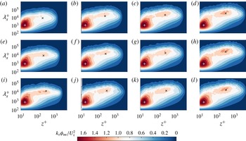
Figure 9 shows pre-multiplied spectra of streamwise velocity,
 $k_{x}{\it\phi}_{uu}$
, as contour plots for each of the three trips at four streamwise locations, where the streamwise wavelength
 ${\it\lambda}_{x}$
is used. At all
 $x$
locations in figure 9 the similarity of
 $k_{x}{\it\phi}_{uu}/U_{{\it\tau}}^{2}$
is evident near the wall at all but the largest scales. For reference, ‘
 $+$
’ is shown on each plot at
 $z^{+}=15$
and
 ${\it\lambda}_{x}^{+}=1000$
, the reported location of the inner peak in the spectrogram (del Alamo et al.
Reference del Alamo, Jiménez, Zandonade and Moser2004; Hutchins & Marusic Reference Hutchins and Marusic2007a
), which corresponds to the location of the inner peak of
 $\overline{u^{2}}/U_{{\it\tau}}^{2}$
. The agreement seen in this near-wall region reinforces our interpretation that the influence of the wall is identical in these three boundary layers.
In contrast, in the outer region the pre-multiplied spectra are seen to have different characteristics, especially at smaller
 $x$
locations. At Station S1, finite magnitudes of
 $k_{x}{\it\phi}_{uu}$
are present for TR06 and TR10 at higher
 $z^{+}$
than for SP40, consistent with the increased
 $Re_{{\it\tau}}$
values. Hutchins & Marusic (Reference Hutchins and Marusic2007a
) reported that an outer peak in the
 $u$
-spectrogram emerges at higher Reynolds numbers, and its location was later clarified by Mathis, Hutchins & Marusic (Reference Mathis, Hutchins and Marusic2009) to occur at
 $z^{+}\approx 3.9Re_{{\it\tau}}^{1/2}$
and
 ${\it\lambda}_{x}/{\it\delta}\approx 6$
; this location is marked by ‘
 $\times$
’ for reference in all plots. The outer spectral peaks for the SP40 cases here appear to follow this quite well; however, it is noted that controversy remains as to the precise location and scaling of this outer spectral peak (see for example, Rosenberg et al.
Reference Rosenberg, Hultmark, Vallikivi, Bailey and Smits2013; Vallikivi, Ganapathisubramani & Smits Reference Vallikivi, Ganapathisubramani and Smits2015) and the mark ‘
 $\times$
’ is used here purely as a reference for three flows.
At Station S1 the outer peak is minimal for the SP40 configuration due to the low Reynolds number at this location. However, an outer peak does appear for the TR06 and TR10 configurations (more prominent for the TR10), but with the additional contributions being of shorter wavelength (closer to
 ${\it\lambda}_{x}^{+}\approx 3Re_{{\it\tau}}$
), and seemingly occurring close to the wall. These additional contributions explain the increased
 $\overline{u^{2}}/U_{{\it\tau}}^{2}$
observed in figure 6, and are consistent with the notion that the bigger trips have artificially aged and thickened the boundary layers. It is noted that the peak for TR10 appears distinctly while that for TR06 resembles a plateau that is connected to the inner peak. As the flows evolve downstream the outer peaks for the three flows seem to converge, and by Station S8 the spectrograms for all three trips appear similar in shape and magnitude.
Pre-multiplied spectra of the streamwise velocity signal for the three trips. Each row is for a particular trip: (a–d) SP40, (e–h) TR06, (i–l) TR10. Each column is for a particular
 $x$
location: (a,e,i) S1, (b,f,j) S4, (c,g,k) S6, (d,h,l) S8.
 $+$
indicates
 ${\it\lambda}_{x}^{+}=1000$
and
 $z^{+}=15$
, while
 $\times$
indicates
 ${\it\lambda}_{x}/{\it\delta}=6$
and
 $z^{+}=3.9Re_{{\it\tau}}^{1/2}$
.

It is deduced that the presence of a threaded rod at the trip location introduces large-scale disturbances in the low-
 $Re$
boundary layer. These large-scale disturbances reside predominantly in the outer part of the boundary layer. A possible explanation is that these large scales either originate from or are amplified by the periodic shedding of the wake behind the rod. The presence of such energetic motions due to the abrupt tripping of the boundary layer is manifested as the outer peak in the spectrogram at low
 $Re_{x}$
, while at the same
 $Re_{x}$
such large scales are absent in the SP40 case.
Excess energy content seen in pre-multiplied spectra of the streamwise velocity signal. Each column is for a particular
 $x$
location: S1 (a,c) and S8 (b,d). Each row is for a particular difference between trip configurations: TR06 – SP40 (a,b) and TR10 – SP40 (c,d). Colour-bar levels indicate differences in
 $k_{x}{\it\phi}_{uu}/U_{{\it\tau}}^{2}$
.

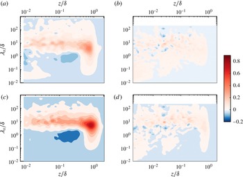
The differences observed between different trip configurations for the pre-multiplied spectra in figure 9 can be more clearly studied if we consider the difference in magnitude of
 $k_{x}{\it\phi}_{uu}$
at matched
 $Re_{x}$
and at a particular
 $z$
and
 ${\it\lambda}_{x}$
. Such differences are plotted in figure 10. Figure 10(a) shows contours of the difference in
 $k_{x}{\it\phi}_{uu}$
between the SP40 and TR06 configurations at Station S1. The dimensional magnitude of
 $k_{x}{\it\phi}_{uu}$
is determined at a wall-normal height
 $z$
and wavelength
 ${\it\lambda}_{x}$
for the SP40 and TR06 spectrograms. Thereafter the magnitude of SP40 is subtracted from that of TR06. The result is non-dimensionalised using
 ${\it\delta}$
and
 $U_{{\it\tau}}$
of the SP40 configuration at Station S1. Similarly, figure 10(c) plots contours of the differences in spectrograms between SP40 and TR10 at Station S1, again utilising parameters of SP40 for non-dimensionalisation. It is clearly seen that the TR06 and TR10 configurations have significant excess kinetic energy in the outer region at Station S1. This excess energy is present in a wide range of scales
 $0.1\leqslant {\it\lambda}_{x}/{\it\delta}\leqslant 100$
but pre-dominantly concentrated near
 ${\it\lambda}_{x}/{\it\delta}\approx 10$
, with the peak difference occurring at
 ${\it\lambda}_{x}/{\it\delta}\approx 6$
,
 $z/{\it\delta}\approx 0.8$
, placing it well into the intermittent region of the boundary layer that typically spans
 $0.4\leqslant z/{\it\delta}\leqslant 1$
. Thus the threaded rod trips significantly influence the intermittent region of the boundary layer by introducing large-scale motions in this region. The excess of energy is larger for TR10 than for TR06, implying that the physical dimensions of the trip have a direct influence on the turbulence in the outer region. These observations for the scale-wise energy content in the outer part complement the observations for the changes in the mean velocity and streamwise normal stress seen earlier. The small increase in the near-wall peak of
 $\overline{u^{2}}/U_{{\it\tau}}^{2}$
for TR10 at Station S1 is seen to come from the introduced large scales penetrating all the way down to the wall. This additional large-scale energy in the near-wall region is likely to also play a role in modulating the small scales near the wall (Mathis et al.
Reference Mathis, Hutchins and Marusic2009; Ganapathisubramani et al.
Reference Ganapathisubramani, Hutchins, Monty, Chung and Marusic2012). An additional interesting feature to note in figure 10(a,c) is the region of reduced energy in the vicinity of
 ${\it\lambda}_{x}/{\it\delta}\approx 0.7$
and
 $z/{\it\delta}\approx 0.2$
. This decrease in energy for the large scales near the outer edge of the log-region is not understood yet, but suggests a transfer of energy at the edge of the log-layer from wavelengths of order
 ${\it\delta}$
to much longer wavelengths.
Complementary to figure 10(a,c) we show the difference in scale-wise energy content at Station S8 in figure 10(b,d). As one would anticipate based on the agreement of mean velocity profiles in figure 5(a), variance in figure 6 and the spectrogram in figure 9(d,h,l), the differences in energy content at any particular wavelength are now quite small. However, for TR10, at Station S8, there is still a clearly observable, though now weakened, region of excess energy centred in the range
 ${\it\lambda}_{x}/{\it\delta}\approx 6{-}10$
and extending from the wall to the edge of the layer.
4.5. Higher-order moments
Above, we have observed that the effects of ‘over-tripping’ diminish as the boundary layers develop over the length of the plate, and as seen in figures 5 and 6, the second-order statistics appear to agree for different trips once both the mean velocity and defect velocities converge to the same respective profiles. This is perhaps surprising as one might intuitively expect that a higher-order statistic would require a longer development length to recover from a perturbed state (i.e
 $\overline{u^{2}}$
should be more sensitive than
 $U$
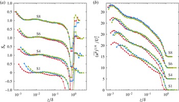
). As noted above, this does not appear to be the case. To test this further we consider higher-order statistics up to tenth order, but for brevity we only show the third- and eighth-order statistics to document the representative trends. These results are shown in figure 11 in the form of the skewness
 $S_{u}=\overline{u^{3}}/(\overline{u^{2}})^{3/2}$
, and
 $(\overline{u^{8}})^{1/4}$
following the work of Meneveau & Marusic (Reference Meneveau and Marusic2013), who showed that even moments represented in this way have a logarithmic behaviour with distance from the wall in the log-region of fully developed ZPG flows, and this is seen to be the case for the SP40 profiles. Comparison between the profiles in figures 11 and 6 indicates that the recovery length required for the statistics to become independent of the trip is not dependent on the order of the statistic (at least not up to tenth order), with all statistics nominally agreeing by Station S8. This suggests that while the larger trips introduce additional length scales into the flow, these perturbations and interactions relax as the boundary layer evolves downstream, and once they have decayed to the point of not further influencing the mean velocity profiles, their influence also appears to be negligible for the higher-order statistics. This finding implies that in order to determine if a flow has sufficiently recovered from a trip and reached a canonical ZPG boundary layer state, then only information about the evolution of the mean velocity profile is required. This is particularly advantageous as a reliable computation scheme can be developed for mean flow evolution, and this is considered in the following section.
Comparison of skewness,
 $S_{u}=\overline{u^{3}}/(\overline{u^{2}})^{3/2}$
, and
 $\overline{u^{8}}$
for the three trips at four streamwise locations. ●, SP40; ▴, TR06; ▪, TR10. Note the vertical shift in profiles.

5. Computing the evolution of turbulent boundary layers
The evolution of the mean flow for ZPG turbulent boundary layers at high Reynolds numbers can be computed in a number of ways, the most common approaches being RANS (Reynolds-averaged Navier–Stokes), CFD and large-eddy simulation. In those cases, however, models with multiple parameters are required together with a chosen grid, and the computations yield velocity profiles. Here, we are interested in mean flow parameters themselves (i.e. shape factor
 $H$
, Coles wake factor
 ${\it\Pi}$
etc.) and these can be directly computed using an integral equation approach described by Perry et al. (Reference Perry, Marusic and Jones2002). For this one requires a closure formulation for the unknown Reynolds shear stresses to solve the Reynolds-averaged Navier–Stokes equations, and here we adopt a scheme similar to that developed by Perry et al. (Reference Perry, Marusic and Li1994). Jones, Marusic & Perry (Reference Jones, Marusic and Perry2001) utilised such a closure formulation to evaluate the development of sink-flow boundary layers and showed good agreement of the calculated evolution with experiments. The objective here is to use the same set of closure formulations to compute the evolution of a boundary layer under zero pressure gradient from a given set of initial conditions.
The procedure involves the hypothesis that the total shear stress profile is uniquely described by a two-parameter family for a zero-pressure-gradient flow. In addition, a relation between the mean flow and shear stress parameters is required to close the system of equations. The equations that govern the streamwise evolution of a turbulent boundary layer can be found after considerable algebra by using the momentum integral and differential equations, the mean continuity equation, the log law of the wall and law of the wake. A more detailed explanation is given in Perry et al. (Reference Perry, Marusic and Li1994, Reference Perry, Marusic and Jones2002) and Jones et al. (Reference Jones, Marusic and Perry2001) and therefore we only summarise the equations relevant to the results presented, for brevity.
5.1. Derivation of evolution equations
As described in Perry et al. (Reference Perry, Marusic and Li1994) and Perry & Marusic (Reference Perry and Marusic1995), the total shear stress profile can be based on four non-dimensional mean flow parameters which describe the state of the turbulent boundary layer:
 $$\begin{eqnarray}\displaystyle {\it\Pi},\quad S=\frac{U_{\infty }}{U_{{\it\tau}}},\quad {\it\beta}=\frac{{\it\delta}^{\ast }}{{\it\tau}_{0}}\frac{\text{d}p}{\text{d}x},\quad {\it\zeta}=S{\it\delta}\frac{\text{d}{\it\Pi}}{\text{d}x}. & & \displaystyle\end{eqnarray}$$
Here
 ${\it\Pi}$
is the wake parameter,
 $S$
is the skin friction parameter,
 ${\it\beta}$
is the pressure gradient parameter, where
 $p$
is the mean static pressure, and
 ${\it\zeta}$
is the non-equilibrium parameter. These parameters come from the mean momentum equation with the assumption that the mean velocity deficit profile is defined as a two-parameter family of the following form:
 $$\begin{eqnarray}\displaystyle \frac{U_{\infty }-U}{U_{{\it\tau}}}=f\left(\frac{z}{{\it\delta}},{\it\Pi}\right). & & \displaystyle\end{eqnarray}$$
A coupled set of ordinary differential equations results (see Jones et al. Reference Jones, Marusic and Perry2001):
 $$\begin{eqnarray}\displaystyle {\displaystyle \frac{\text{d}S}{\text{d}Re_{x}}} & = & \displaystyle {\displaystyle \frac{{\it\chi}[Re_{x},K]~R[S,{\it\Pi},{\it\zeta},{\it\beta}]}{S\;E[{\it\Pi}]\;\exp [{\it\kappa}S]}},\end{eqnarray}$$
 $$\begin{eqnarray}\displaystyle {\displaystyle \frac{\text{d}{\it\Pi}}{\text{d}Re_{x}}} & = & \displaystyle {\displaystyle \frac{{\it\zeta}~{\it\chi}[Re_{x},K]}{S^{2}\;E[{\it\Pi}]\;\exp [{\it\kappa}S]}}.\end{eqnarray}$$
 $R[S,{\it\Pi},{\it\zeta},{\it\beta}]$
and
 $E[{\it\Pi}]$
are given in detail in Jones et al. (Reference Jones, Marusic and Perry2001) and Perry et al. (Reference Perry, Marusic and Jones2002). Also,
 $$\begin{eqnarray}\displaystyle & \displaystyle {\it\chi}[R_{x},K]=U_{\infty }(x)/U_{0}, & \displaystyle\end{eqnarray}$$
 $$\begin{eqnarray}\displaystyle & \displaystyle K=\frac{{\it\nu}}{U_{\infty }^{2}}\frac{\text{d}U_{\infty }}{\text{d}x}=0, & \displaystyle\end{eqnarray}$$
 $U_{0}$
is the reference free-stream velocity (free-stream velocity at the streamwise location of the trip, i.e.
 $U_{0}=U_{\infty }[x=0]$
). In the case of ZPG flows
 $U_{0}=U_{\infty }$
,
 ${\it\beta}=0$
and
 $K=0$
since
 $\text{d}U_{\infty }/\text{d}x$
= 0. Therefore, in summary, the evolution equations (5.3) and (5.4) are functions of three mean flow parameters only:
 $S,{\it\Pi}\text{ and }{\it\zeta}$
. However, this leaves two equations with three unknowns. In order to close this problem, there needs to be one more equation, and in the absence of new theory that equation must be obtained empirically as a function of
 $S,{\it\Pi}\text{ and }{\it\zeta}$
. This semi-empirical equation is termed the ‘closure equation’.
Total shear stress profiles computed using the closure formulation of Perry et al. (Reference Perry, Marusic and Li1994) for varying values of
 $S=U_{\infty }/U_{{\it\tau}}$
.

5.2. Closure formulation for ZPG flows
The restricted formulation of Perry et al. (Reference Perry, Marusic and Li1994) will now be extended with the effect of the parameter
 ${\it\zeta}$
included so that the non-equilibrium flow problem can be solved. Hence, following Perry et al. (Reference Perry, Marusic and Jones2002),
 $$\begin{eqnarray}\displaystyle F[{\it\Pi},S,{\it\beta},{\it\zeta}]=0\quad \Rightarrow \quad F[{\it\Pi},S,{\it\zeta}]=0. & & \displaystyle\end{eqnarray}$$
It is assumed that no further parameters are involved in (5.7) and
 $F$
is universal. Mapping out (5.7) from experimental data would help us to find the state of the developing boundary layer. As mentioned previously, the shear stress profile can be expressed by using these three mean flow parameters,
 ${\it\Pi}$
,
 $S$
and
 ${\it\zeta}$
. Figure 12 clearly shows that the variation of shear stress profiles with
 $S$
is only marginal, even over a very large range of
 $S$
. Since all the experimental data fall between
 $S$
values of 20 to 40, it is very clear that we can approximate that the influence of
 $S$
is small. Therefore, the variation in
 $S$
is neglected and (5.7) is reduced to a two-parameter family of the following form:
 $$\begin{eqnarray}F[{\it\Pi},{\it\zeta}]\approx 0,\end{eqnarray}$$
or
 $$\begin{eqnarray}{\it\zeta}=f[{\it\Pi}],\end{eqnarray}$$
which we will attempt to find empirically.
5.3. Log-law of the wall and wake formulation
Before determining the functional form of (5.9) a note on the definition of
 ${\it\Pi}$
is necessary. One can find many log-law of the wall and wake formulations in the literature, e.g. Coles (Reference Coles1956), Moses (Reference Moses1964), Lewkowicz (Reference Lewkowicz1982), Jones (Reference Jones1998), Nickels (Reference Nickels2004) and more recently Chauhan et al. (Reference Chauhan, Nagib and Monkewitz2009). As described earlier, the composite profile of Chauhan et al. (Reference Chauhan, Nagib and Monkewitz2009) was used to fit the experimental data in order to obtain the parameters
 ${\it\Pi}$
,
 ${\it\delta}$
and
 $U_{{\it\tau}}$
, and therefore for consistency we continue to use their wall-wake formulation here, which is given by
 $$\begin{eqnarray}\displaystyle \frac{U}{U_{{\it\tau}}}=U_{inner}^{+}(z^{+})+\frac{2{\it\Pi}}{{\it\kappa}}W(z/{\it\delta}),\quad 0\leqslant z\leqslant {\it\delta}, & & \displaystyle\end{eqnarray}$$
where the inner function is essentially the near-wall formulation of Musker (Reference Musker1979) that approaches the logarithmic law with slope
 ${\it\kappa}=0.384$
and additive constant
 $B=4.17$
in the range
 $z^{+}\geqslant 100$
, and the wake function
 $W$
takes the form of an exponential function. It should be noted, however, that any convenient formulation of the logarithmic profile coupled with a wake function can be used in the closure formulation of Perry et al. (Reference Perry, Marusic and Li1994) and Perry & Marusic (Reference Perry and Marusic1995). The parameter
 ${\it\Pi}$
in the theory is not bound to a particular choice of wake function.
5.4. Functional form for ‘closure’ equation
In order to evaluate the evolution of the ZPG boundary layer a general expression is required for (5.9), i.e.
 $$\begin{eqnarray}{\it\zeta}=f\,[{\it\Pi}].\end{eqnarray}$$
Although the attached eddy model of Perry et al. (Reference Perry, Marusic and Li1994) can assist us for quasi-equilibrium flows, at the present time we still require a model for finite
 ${\it\zeta}$
values. The answer can be found empirically provided enough experimental information is available. Here we require experiments where a constant free-stream velocity
 $U_{\infty }$
was maintained at different streamwise stations
 $x$
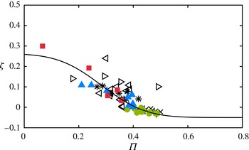
to obtain different Reynolds numbers, and unfortunately only a limited number of previous studies satisfy this requirement. In figure 13 we compile data that is available from the studies of Klebanoff & Diehl (Reference Klebanoff and Diehl1951), Erm (Reference Erm1988), Nagano, Tagawa & Tsuji (Reference Nagano, Tagawa and Tsuji1993) and Österlund (Reference Österlund1999), together with the present data from the three trips. A curve fit to (5.11) is obtained, given by
 $$\begin{eqnarray}\displaystyle {\it\zeta}=0.1862\times \text{erfc}[({\it\Pi}-0.2544)\times 4.935]-0.0517. & & \displaystyle\end{eqnarray}$$
Here the flow cases that have
 ${\it\zeta}>0$
are identified as developing flows and the flow cases where
 ${\it\zeta}<0$
are identified as relaxing flows. Previously Perry et al. (Reference Perry, Marusic and Jones2002) proposed two closure equations corresponding to the relaxing and developing cases but it is deemed unnecessary for ZPG flow to have two functional forms for (5.11), as it is evident from figure 13 that all the discrete data appear to agree reasonably well with the proposed fit (5.12).
Variation of the non-equilibrium parameter
 ${\it\zeta}$
with wake parameter
 ${\it\Pi}$
for experimental ZPG boundary layer measurements. Symbols are:
 $\ast$
, Erm (Reference Erm1988); ▹, Klebanoff & Diehl (Reference Klebanoff and Diehl1951); ◃, Nagano et al. (Reference Nagano, Tagawa and Tsuji1993);
 $\times$
,
 $U_{\infty }=37~\text{m}~\text{s}^{-1}$
data of Österlund (Reference Österlund1999);
 $+$
,
 $U_{\infty }=42~\text{m}~\text{s}^{-1}$
data of Österlund (Reference Österlund1999); ●, SP40; ▴, TR06; ▪, TR10. Solid line is (5.12).

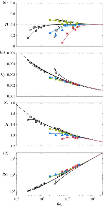
Comparison of experimental boundary layer parameters with computed evolution. (a)
 ${\it\Pi}$
versus
 $Re_{x}$
. Dashed line is the asymptotic limit of
 ${\it\Pi}$
according to the definition of Chauhan et al. (Reference Chauhan, Nagib and Monkewitz2009);
 ${\it\Pi}\rightarrow 0.42$
; (b)
 $C_{f}$
versus
 $Re_{x}$
. Dashed line is Schlichting’s fit,
 $C_{f}=[2\log _{10}(Re_{x})-0.65]^{-7/3}$
; (c)
 $H$
versus
 $Re_{x}$
. Dashed line is
 $H=(1-7.1/\sqrt{2/C_{f}})^{-1}$
; (d)
 $Re_{{\it\theta}}$
versus
 $Re_{x}$
. See figure 13 for explanation of symbols.

6. Comparison of computed evolution with experimental data
When comparing results from different sources it is important to have consistent definitions for the various measured quantities. Thus, in an effort to ease comparability, certain parameters such as
 ${\it\delta},U_{{\it\tau}},H\text{ and }C_{f}$
have been recomputed in a consistent manner for all data sets presented in this study. This is particularly important for the wake parameter
 ${\it\Pi}$
. Figure 14 shows the evolution of mean flow parameters compared with the predicted evolution solution computed using (5.3), (5.4) and (5.12). All measurements shown here were taken at a nominally constant free-stream velocity (
 $U_{\infty }$
) and the increase in Reynolds number is achieved by increasing
 $x$
. In order to compute the analytical evolution, the initial conditions for
 ${\it\Pi}$
and
 $S$
have to be specified, and this is done at the lowest-Reynolds-number measurement in a particular data set. For example, the initial conditions of the lowest-Reynolds-number measurement (at
 $Re_{{\it\tau}}=2730$
) are assigned to compute the analytical evolution for the tripping configuration SP40.
Figure 14(a) shows the evolution of
 ${\it\Pi}$
and good agreement is observed between the experimental data and the computed evolutions (solid lines). For SP40, the flow is seen to be relaxing because the wake parameter starts at a slightly higher value initially and then approaches a constant as
 $Re_{x}$
increases. This could be because the mean height of the roughness elements on the sandpaper trip are smaller than the incoming boundary layer height and therefore the transition is triggered within the layer, resulting in a weakly under-stimulated boundary layer (or the development of an internal layer). A cursory inspection of the mean velocity profiles does not seem to indicate this behaviour; however, the computed evolution captures this relaxing tendency very clearly. In the TR10 and TR06 cases, the flows are developing and as the Reynolds number increases the
 ${\it\Pi}$
values increase and approach a constant. For both these trips the transition is triggered by introducing large-scale perturbations emerging from the wake behind the threaded rod. Thereby, the relative size of these perturbations is of the same order as the incoming boundary layer thickness. Hence these trips over-stimulate the flow and have fuller velocity profiles, resulting initially in smaller wake regions.
It is noted that the results in figure 14(a) show that even by Station S8 (
 $Re_{x}\approx 2\times 10^{7}$
) the
 ${\it\Pi}$
values have not yet strictly converged. The computed evolution curves indicate that for the
 ${\it\Pi}$
values for the three tripping configurations to all agree within 4 % requires
 $Re_{x}\approx 7\times 10^{7}$
(corresponding to
 $U_{\infty }^{+}$
 ${\approx}$
33 and
 $x\approx 54~\text{m}$
), which is well beyond the length of the facility. These results indicate that the trip does have a considerable effect in the wake region, not only for the low-Reynolds-number flows as suggested by Coles (Reference Coles1962) and Erm & Joubert (Reference Erm and Joubert1991), but also at substantial
 $Re_{x}$
. According to Coles (Reference Coles1962),
 ${\it\Pi}$
is observed to drop for
 $Re_{{\it\delta}^{\ast }}<$
5000, and he described this as a low-Reynolds-number effect. However, here we see that this trend is better described as an evolution effect resulting from the initial conditions set up by the trip and/or the initial inflow conditions.
Also shown in figure 14(a) is the computed evolution for the data of Klebanoff & Diehl (Reference Klebanoff and Diehl1951), Erm (Reference Erm1988), Nagano et al. (Reference Nagano, Tagawa and Tsuji1993) and Österlund (Reference Österlund1999). In the case of Österlund’s
 $32~\text{m}~\text{s}^{-1}$
data and
 $43~\text{m}~\text{s}^{-1}$
data, the flow is under-stimulated and the computed evolution predicts the
 ${\it\Pi}$
trend reasonably well. The remaining data have over-stimulated flow and their corresponding development is again well predicted by the computation (solid lines). As a concluding comment for figure 14(a), it is found that any reasonable definition of
 ${\it\Pi}$
used in the analysis of the experimental profiles does not change the trends seen in the figure, but only results in some shift in magnitude (value of
 ${\it\Pi}$
) (see Chauhan, Nagib & Monkewitz Reference Chauhan, Nagib and Monkewitz2007).
Figures 14(b), 14(c) and 14(d) show, respectively, the variation of friction coefficient
 $C_{f}=2(U_{{\it\tau}}/U_{\infty })^{2}$
, shape factor
 $H={\it\delta}^{\ast }/{\it\theta}$
, and Reynolds number based on momentum thickness,
 $Re_{{\it\theta}}$
, versus
 $Re_{x}$
, and again all the experiments considered in this study agree well with the computed evolution. The dashed line in figure 14(b) is Schlichting’s relation modified according to Nagib et al. (Reference Nagib, Chauhan and Monkewitz2007); given as
 $C_{f}=[2\log _{10}(Re_{x})-0.65]^{-7/3}$
(Schlichting Reference Schlichting1960). Tripping configurations TR10 and TR06, where the flow is over-tripped, as well as SP40, where the boundary layer seems to be under-stimulated, exhibit behaviour that deviates from the canonical ZPG case at low
 $Re_{x}$
. A distinctly noticeable deviation of
 $C_{f}$
from the canonical behaviour is also observed for the data of Klebanoff & Diehl (Reference Klebanoff and Diehl1951) (where a 0.04 in. rod was used as the trip). However, even in these cases the computed evolution still accurately predicts the
 $C_{f}$
development.
The shape factor
 $H$
is an integral parameter that can be considered as an independent criterion, since it offers a direct assessment of measured profiles without any assumptions or reliance on theory and independent wall-shear measurements. Figure 14(c) also shows the comparison between the equation for
 $H$
provided in Chauhan et al. (Reference Chauhan, Nagib and Monkewitz2009) and the computed evolution for different experiments. The data points for Erm (Reference Erm1988) at low Reynolds number deviate from the dashed-curve of Chauhan et al. (Reference Chauhan, Nagib and Monkewitz2009) for canonical behaviour of
 $H$
and likewise the non-canonical cases of TR06 and TR10 deviate considerably from the curve at high Reynolds numbers. However, the computed evolution captures the trend of the experimental data quite well. The comparison of Reynolds numbers in figure 14(d) emphasises that there is no one-to-one correspondence between Reynolds numbers as long as the remnants of the initial conditions persists in a given ZPG flow.
While the present experimental results are limited to one free-stream velocity, it is expected that similar qualitative trends will emerge for other free-stream velocities and that an account of the boundary layer evolution is needed in all cases. The overall results in figure 14 highlight that matching one Reynolds number does not guarantee similar states of two different ZPG flows. It is clear that non-equilibrium effects introduced in the boundary layer at any stage not only cause the flow to deviate from the canonical state but also have an influence on its growth immediately downstream at low Reynolds number. The good news, though, is that the above results indicate that the streamwise evolution of ZPG turbulent boundary layers can be computed, provided the appropriate upstream initial conditions are specified.
7. Conclusions
Measurements were performed in the large University of Melbourne wind tunnel to study the spatial evolution of zero-pressure-gradient turbulent boundary layers from their origin to a high-Reynolds-number state. Careful attention was given to the experimental procedures in order to make comparisons between flows with three different trips while keeping all other parameters nominally constant, including the pressure gradient and keeping the measurement sensor size nominally fixed at
 $l^{+}\approx 24$
. The three trips consist of a standard sandpaper trip (SP40) and two cases where additional threaded rods of 6 mm (TR06) and 10 mm (TR10) diameter are added. The SP40 case was regarded as the standard case and measurements at 10 different streamwise stations covering a range
 $2700<Re_{{\it\tau}}<13\,000$
showed good agreement with the known scaling behaviour for mean flow and streamwise Reynolds stresses described in the literature (Smits, McKeon & Marusic Reference Smits, McKeon and Marusic2011). The near-wall peak value in
 $\overline{u^{2}}^{+}$
at
 $z^{+}\approx 15$
is found to follow a log-linear dependence with
 $Re_{{\it\tau}}$
with a slope consistent with that recently reported from DNS results by Lee & Moser (Reference Lee and Moser2015).
Since
 $U_{\infty }/{\it\nu}$
was held constant for all cases, comparisons at matched streamwise distance from the trip (
 $x$
) correspond to matched
 $Re_{x}$
. The TR06 and TR10 cases were found to have significant differences to the SP40 case for
 $U^{+}$
and
 $\overline{u^{2}}^{+}$
at low Reynolds number, particularly in the outer region of the boundary layer, with the larger trip (TR10) resulting in larger deviations from canonical behaviour. Comparisons of spectra reveal that the over-stimulated trips introduce large-scale disturbances into the boundary layer, which are prominent at low
 $Re$
. These large-scale disturbances reside predominantly in the outer part of the boundary layer, and probably originate from or are amplified by the periodic shedding of the wake behind the rod. The presence of such energetic motions due to the abrupt tripping of the boundary layer is manifested as an outer peak in the spectrogram at low
 $Re_{x}$
, while at the same
 $Re_{x}$
such large scales are absent in the SP40 case. This artificial outer peak is different to the naturally occurring outer spectral peak that occurs at high
 $Re$
in canonical ZPG flows. The remnants of the ‘over-tripped’ conditions are seen to persist for some distance, at least until Station S8, at which position the non-canonical boundary layers (TR06 and TR10) exhibit a weak memory of their initial conditions only for the large scales
 $O(10{\it\delta})$
. Generally, the mean velocity profiles were found to approach a constant wake parameter
 ${\it\Pi}$
as the three boundary layers developed along the test section, and the mean flow, broadband turbulence intensities, and higher-order moments are all found to nominally agree by Station S8.
A comparison of
 $U^{+}$
and
 $\overline{u^{2}}^{+}$
was also made at nominally matched local Reynolds numbers, namely at
 $Re_{{\it\tau}}\approx 8000$
and
 $Re_{{\it\theta}}\approx 10\,400$
. In both cases distinct differences were observed despite the matched local Reynolds number, due to the incomplete recoveries of the over-stimulated boundary layers. In these cases it is clear that there is no one-to-one correspondence between
 $Re_{{\it\tau}}$
,
 $Re_{{\it\theta}}$
or
 $Re_{x}$
, and this highlights that caution is needed when comparing data sets obtained under different free-stream velocity conditions to achieve different Reynolds numbers, with little or no information about their initial or upstream boundary conditions. Unfortunately the majority of studies in the literature fall into this category. We find that non-equilibrium effects in the boundary layer are not confined to low Reynolds number, and can persist even at high Reynolds numbers. All ZPG boundary layers would be expected to evolve to an equivalent form where Reynolds-number similarity holds, provided the Reynolds number is sufficiently high, and the larger the trip disturbance is above its ideal trip size the longer the boundary layer will need to recover. However, it is not clear a priori how long this will take and how far downstream of the trip this will occur. For the trips considered in our study, the recovery occurs at
 $Re_{x}\approx 1.7\times 10^{7}$
, which corresponds to a distance along the plate of
 $O(2000)$
trip heights. It is also noted that the present study is restricted to measurements only of the streamwise component of velocity. Seo et al. (Reference Seo, Castillo, Johansson and Hangan2004) have shown that wall-normal component statistics are more sensitive to initial conditions, such as
 $\overline{w^{2}}$
compared to
 $\overline{u^{2}}$
, and this may change the quantitative values of the evolution lengths required to recover from over-tripped conditions, and/or the conclusions regarding statistics of other velocity components.
A perhaps surprising but important finding from the present study is that the recovery length required for the statistics to become independent of the trip is not dependent on the order of the statistic (at least not up to tenth order for
 $u$
). This suggests that, while the larger trips introduce additional length scales into the flow, these perturbations and interactions relax as the boundary layer evolves downstream and once they have decayed to the point of not further influencing the mean velocity profiles, their influence also appears to be negligible for the higher-order statistics. This is at least the case in the present study where the inflow initial conditions are maintained constant and only the trip is varied. This result therefore implies that for streamwise velocity statistics it may be sufficient to document the mean flow parameters alone in order to ascertain whether the ZPG flow has reached a canonical state.
The evolution of the mean flow parameters is considered by computing solutions of the momentum integral equations using a semi-empirical closure relation for ZPG turbulent boundary layers based on a survey of available data. Using this approach, the predicted evolution for all tripped configurations is found to be in agreement with the experimental data for the mean flow parameters such as
 ${\it\Pi}$
,
 $H$
,
 $C_{f}$
for a wide range of Reynolds numbers. From figure 14, it can be seen that, though the local parameters such as the Reynolds number
 $Re_{x}$
are matched (for the sake of Reynolds-number similarity), different mean flow parameters (
 ${\it\Pi}$
,
 $H$
,
 $C_{f}$
) can be obtained. This computational scheme should therefore be useful as a tool towards determining whether a given ZPG boundary layer is of a canonical form.
Acknowledgements
The authors wish to gratefully acknowledge the Australian Research Council for the financial support of this project.