


1 Introduction
Under ‘quiet’ free-stream conditions, the boundary layer on a supersonic or hypersonic body behaves as a convectively unstable waveguide (Fedorov Reference Fedorov2011). To predict the transition onset location one should solve the initial boundary-value problem that requires detailed specification of the ambient disturbance environment. Bushnell (Reference Bushnell, Hussaini and Voigt1990) summarized information on the ambient disturbances for atmospheric flights and pointed out that solid particulates are one of the major sources of disturbance energy. The occurrence of atmospheric particulates is associated with ice clouds, volcanic and other terrestrial dust as well cosmic dust (Turco Reference Turco1992; GAM Guide 1999). A substantial portion of particulates having sizes of the order of
 $10~\unicode[STIX]{x03BC}\text{m}$
consists of the products of rocket exhausts from previous flights. These findings motivated Fedorov (Reference Fedorov2013) to analyse the receptivity problem describing excitation of unstable modes by spherical solid particulates interacting with the laminar flow on a body moving at supersonic speeds. The analysis was focused on the dynamic interaction of particulates with the boundary layer. Effects associated with particulate-induced vortical disturbances, acoustic waves and roughness were not considered. Analytical solutions of the receptivity problem were incorporated into the amplitude method of Mack (Reference Mack1977) to predict the particulate-induced transition onset. As an example, Fedorov (Reference Fedorov2013) carried out computations for a
 $14^{\circ }$
half-angle sharp wedge flying in the standard atmosphere at altitude 20 km, Mach number 4 and zero angle of attack. In this case, transition is associated with instability of the first mode according to the terminology of Mack (Reference Mack1969). It was shown that spherical particulates of radius from
 $10$
to
 $20~\unicode[STIX]{x03BC}\text{m}$
and density greater than
 $1~\text{g}~\text{cm}^{-3}$
can cause the transition onset corresponding to the amplification factor
 $N=9{-}10$
, which is in the empirical range of flight data (Hefner & Bushnell Reference Hefner and Bushnell1979).
Note that flows in many impulse facilities used for ground testing of hypersonic configurations may be heavily contaminated with particulates (diaphragm fragments, rust particles, soot, dust, etc.). Transition measurements in these facilities may be strongly influenced by particulate impacts. For example, Jewell et al. (Reference Jewell2017) showed that a cleaning procedure in a hypervelocity shock tunnel T5 at the California Institute of Technology improves the repeatability of transition measurements. Prior to the implementation of the cleaning regimen, unpredictable turbulent spots were observed at locations uncharacteristic of natural transition. Following the cleaning, these anomalous results have been nearly eliminated.
The theoretical model (Fedorov Reference Fedorov2013) was developed for relatively simple basic flows where the boundary layer is weakly non-parallel. The model exploits asymptotic techniques with the assumption that the local Reynolds number based on the boundary-layer thickness is large. The receptivity problem and the propagation of particulate-induced wavepackets were analysed assuming that the dominant wavelength was small compared to the body length (so called short-wave or Wentzel–Kramers–Brillouin (WKB) approximation). However, in most of practical cases particulates penetrate into the boundary layer near the body nose, where the short-wave approximation is not valid. To avoid the foregoing restrictions and treat more realistic configurations such as blunt bodies, it has been suggested that the numerical component of the model be enhanced. Namely, the analytical solutions are replaced by numerical integration of the full Navier–Stokes equations with the particulate-induced source terms taken from the original analysis (Fedorov Reference Fedorov2013). The theoretical (Fedorov Reference Fedorov2013) and numerical (present paper) approaches are cross-validated by detail comparisons of the wavepacket characteristics.
The paper is organized as follows. In § 2, we briefly outline the theoretical model (Fedorov Reference Fedorov2013) and set a problem to be solved numerically. In § 3, we discuss the numerical method and formulate requirements for the computational grid and other parameters by solving test problems. In § 4, we discuss numerical results for a particulate-induced wavepacket on a sharp wedge at the free-stream Mach number 4, evaluate their accuracy and compare them with the theoretical solution. In § 5, we conclude the paper with a summary discussion.
2 Governing equations and the theoretical solution
Consider a laminar flow past a sharp wedge in a supersonic free stream of speed
 $U_{\infty }^{\ast }$
, density
 $\unicode[STIX]{x1D70C}_{\infty }^{\ast }$
and temperature
 $T_{\infty }^{\ast }$
(figure 1). Hereafter asterisks denote dimensional quantities and ‘
 $\infty$
’ marks free-stream quantities. The inviscid shock layer between the bow shock and the wedge surface is assumed to be much thicker than the viscous boundary layer; i.e. the Reynolds number based on the wedge length and the free-stream parameters is large. Neglecting the viscous–inviscid interaction, the inviscid shock-layer flow is assumed to be uniform and of constant velocity
 $\boldsymbol{U}_{2}^{\ast }$
, density
 $\unicode[STIX]{x1D70C}_{2}^{\ast }$
, temperature
 $T_{2}^{\ast }$
and pressure
 $P_{2}^{\ast }$
. At the initial time instant
 $t^{\ast }=t_{0}^{\ast }$
, a solid spherical particulate of density
 $\unicode[STIX]{x1D70C}_{p}^{\ast }$
and radius
 $R_{p}^{\ast }$
crosses the shock at a point
 $\boldsymbol{r}^{\ast }=\boldsymbol{r}_{0}^{\ast }$
, where
 $\boldsymbol{r}^{\ast }=(r_{1}^{\ast },r_{2}^{\ast },r_{3}^{\ast })$
is shown in figure 1. Hereafter the subscript ‘
 $p$
’ denotes a particulate quantity.
Schematic of a supersonic flow past a sharp wedge and the coordinate systems. BL stands for the upper boundary-layer edge.

In the shock layer, the particulate dynamics is governed by the equations
 $$\begin{eqnarray}\displaystyle & \displaystyle m_{p}^{\ast }\frac{\text{d}\boldsymbol{u}_{p}^{\ast }}{\text{d}t^{\ast }}=\boldsymbol{F}_{p}^{\ast }, & \displaystyle\end{eqnarray}$$
 $$\begin{eqnarray}\displaystyle & \displaystyle \boldsymbol{u}_{p}^{\ast }(t_{0}^{\ast })=(U_{\infty }^{\ast },0,0)^{\text{T}}, & \displaystyle\end{eqnarray}$$
where
 $\boldsymbol{u}_{p}^{\ast }=\text{d}\boldsymbol{r}_{p}^{\ast }/\text{d}t$
is particulate velocity,
 $m_{p}^{\ast }=4\unicode[STIX]{x03C0}R_{p}^{\ast 3}\unicode[STIX]{x1D70C}_{p}^{\ast }/3$
is particulate mass and
 $\boldsymbol{F}_{p}^{\ast }$
is the drag force. The gravitational force is neglected. The flow past the particulate is treated as quasi-steady, and the drag is calculated as
 $$\begin{eqnarray}\displaystyle \boldsymbol{F}_{p}^{\ast }=-C_{D}\frac{\unicode[STIX]{x1D70C}^{\ast }}{2}|\boldsymbol{u}_{p}^{\ast }-\boldsymbol{u}^{\ast }|(\boldsymbol{u}_{p}^{\ast }-\boldsymbol{u}^{\ast })\unicode[STIX]{x03C0}R_{p}^{\ast 2}. & & \displaystyle\end{eqnarray}$$
The drag coefficient
 $C_{D}$
is computed using the empirical correlation of Crowe (Reference Crowe1967). If the particulate radius is much smaller than the boundary-layer thickness near the particulate impact on the body surface,
 $R_{p}^{\ast }\ll \unicode[STIX]{x1D6FF}^{\ast }$
, then the problem (2.1)–(2.2) describes the particulate passage through the viscous boundary layer also.
By solving (2.1)–(2.3) we can determine the particulate velocity
 $\boldsymbol{u}_{pw}^{\ast }\equiv \boldsymbol{u}_{c}^{\ast }$
at the collision point and then assume that the particulate passes through the thin boundary layer at constant speed
 $\boldsymbol{u}_{pw}^{\ast }$
. Hereafter the subscript ‘
 $w$
’ stands for ‘wall’, while ‘
 $c$
’ refers to the collision point. Preliminary computations of the particle trajectory showed that, in the case considered hereafter, the speed
 $\boldsymbol{u}_{p}^{\ast }$
decreases by less than 0.25 % as the particulate crosses the boundary layer.
For simplicity, let the particulate stick to the wall upon the collision. Effects related to the particulate-induced roughness or the particulate rebound, are not considered. Note that the wall surface can be treated as aerodynamically smooth if the roughness Reynolds number
 $Re_{kk}\equiv ku_{k}/\unicode[STIX]{x1D708}_{k}<25$
, where
 $u_{k}$
and
 $\unicode[STIX]{x1D708}_{k}$
are the velocity and kinematic viscosity in the undisturbed boundary layer at the roughness height
 $k$
(Schneider Reference Schneider2008). The cases considered hereafter satisfy this restriction (Fedorov Reference Fedorov2013). Moving through the boundary layer, the particulate generates flow disturbances (including unstable modes) in a local region where the unperturbed laminar flow can be treated as locally parallel (see figure 1).
A small particulate induces concentrated sources of force and heat (if the particulate surface is not in thermal equilibrium with the ambient flow). The source terms are included in the Navier–Stokes equations for a calorically perfect gas. These equations are written in the dimensionless form
 $$\begin{eqnarray}\displaystyle & \displaystyle \frac{\unicode[STIX]{x2202}\unicode[STIX]{x1D70C}}{\unicode[STIX]{x2202}t}+\frac{\unicode[STIX]{x2202}}{\unicode[STIX]{x2202}r_{j}}(\unicode[STIX]{x1D70C}u_{j})=0, & \displaystyle\end{eqnarray}$$
 $$\begin{eqnarray}\displaystyle & \displaystyle \frac{\unicode[STIX]{x2202}}{\unicode[STIX]{x2202}t}(\unicode[STIX]{x1D70C}u_{i})+\frac{\unicode[STIX]{x2202}}{\unicode[STIX]{x2202}r_{j}}(\unicode[STIX]{x1D70C}u_{i}u_{j}+p\unicode[STIX]{x1D6FF}_{ij})=\frac{1}{Re}\frac{\unicode[STIX]{x2202}\unicode[STIX]{x1D70F}_{ij}}{\unicode[STIX]{x2202}r_{j}}+R_{p}^{2}\bar{F}_{pi}\unicode[STIX]{x1D6FF}(\boldsymbol{r}-\boldsymbol{r}_{p}), & \displaystyle\end{eqnarray}$$
 $$\begin{eqnarray}\displaystyle \unicode[STIX]{x1D70C}\left[\frac{\unicode[STIX]{x2202}T}{\unicode[STIX]{x2202}t}+u_{j}\frac{\unicode[STIX]{x2202}T}{\unicode[STIX]{x2202}r_{j}}\right] & = & \displaystyle \frac{1}{Pr\,Re}\frac{\unicode[STIX]{x2202}}{\unicode[STIX]{x2202}r_{j}}\left(\unicode[STIX]{x1D707}\frac{\unicode[STIX]{x2202}T}{\unicode[STIX]{x2202}r_{j}}\right)+(\unicode[STIX]{x1D6FE}-1)M_{\infty }^{2}\left(\frac{\unicode[STIX]{x2202}p}{\unicode[STIX]{x2202}t}+u_{j}\frac{\unicode[STIX]{x2202}p}{\unicode[STIX]{x2202}r_{j}}\right)+\frac{(\unicode[STIX]{x1D6FE}-1)M_{\infty }^{2}}{Re}\unicode[STIX]{x1D6F7}\nonumber\\ \displaystyle & & \displaystyle +\,\frac{R_{p}}{Pr\,Re}\bar{Q}_{p}\unicode[STIX]{x1D6FF}(\boldsymbol{r}-\boldsymbol{r}_{p})+R_{p}^{2}(\unicode[STIX]{x1D6FE}-1)M_{\infty }^{2}(u_{pj}-u_{j})\bar{F}_{pj}\unicode[STIX]{x1D6FF}(\boldsymbol{r}-\boldsymbol{r}_{p}),\end{eqnarray}$$
 $$\begin{eqnarray}\displaystyle \unicode[STIX]{x1D6FE}M_{\infty }^{2}p=\unicode[STIX]{x1D70C}T, & & \displaystyle\end{eqnarray}$$
where the velocity components
 $u_{j}$
, density
 $\unicode[STIX]{x1D70C}$
, temperature
 $T$
and pressure
 $p$
are scaled using their free-stream values
 $U_{\infty }^{\ast }$
,
 $\unicode[STIX]{x1D70C}_{\infty }^{\ast }$
,
 $T_{\infty }^{\ast }$
and
 $\unicode[STIX]{x1D70C}_{\infty }^{\ast }U_{\infty }^{\ast 2}$
, respectively. The length scale
 $L^{\ast }$
is of the order of the wedge length, the time scale is
 $L^{\ast }/U_{\infty }^{\ast }$
, the Reynolds number is
 $Re=\unicode[STIX]{x1D70C}_{\infty }^{\ast }U_{\infty }^{\ast }L^{\ast }/\unicode[STIX]{x1D707}_{\infty }^{\ast }$
and the Mach number is
 $M_{\infty }=U_{\infty }^{\ast }/a_{\infty }^{\ast }$
, where
 $a$
is the speed of sound. The momentum equation (2.5) contains the particulate-induced force components
 $R_{p}^{2}\bar{F}_{pi}\unicode[STIX]{x1D6FF}(\boldsymbol{r}-\boldsymbol{r}_{p})$
, where
 $\unicode[STIX]{x1D6FF}(\boldsymbol{r}-\boldsymbol{r}_{p})$
is three-dimensional Dirac delta function, and
 $$\begin{eqnarray}\displaystyle \bar{F}_{pi}=C_{D}\frac{\unicode[STIX]{x1D70C}}{2}\unicode[STIX]{x03C0}|\boldsymbol{u}-\boldsymbol{u}_{p}|(u_{ip}-u_{i}). & & \displaystyle\end{eqnarray}$$
The energy equation (2.6) contains the dissipation function
 $\unicode[STIX]{x1D6F7}$
, the particulate-induced energy source proportional to
 $\bar{Q}_{p}=2\unicode[STIX]{x03C0}Nu(T_{p}-T)$
, where
 $Nu$
is the Nusselt number, and the power source term proportional to
 $(u_{pj}-u_{j})\bar{F}_{pj}$
.
In the theoretical analysis (Fedorov Reference Fedorov2013), the flow field is expressed as
 $$\begin{eqnarray}\displaystyle q(x,y,z,t)=Q(x,y,z)+R_{p}^{2}\tilde{q}(x,y,z,t), & & \displaystyle\end{eqnarray}$$
where the Cartesian coordinate system
 $(x,y,z)$
is shown in figure 1,
 $q$
is a certain physical quantity (e.g. the wall pressure),
 $Q$
is the unperturbed basic flow and
 $R_{p}^{2}\tilde{q}=q^{\prime }$
is the particulate-induced disturbance.
Because the dimensionless radius of particulate is small,
 $R_{p}\ll 1$
, the disturbance is governed by the linearized Navier–Stokes equations in the first-order approximation with respect to
 $R_{p}^{2}$
. In this framework, the receptivity problem is solved using the biorthogonal eigenfunction decomposition method. If the particulate hits the wall at the point
 $(x,y,z)=(x_{c},0,0)$
and time instant
 $t=0$
, the particulate-induced disturbance related to mode
 $m$
is expressed as
 $$\begin{eqnarray}\displaystyle & & \displaystyle x>x_{c}:\quad \tilde{q}(x,y,z,t)\nonumber\\ \displaystyle & & \displaystyle \quad =\frac{1}{(2\unicode[STIX]{x03C0})^{2}}\int _{-\infty }^{\infty }\int _{-\infty }^{\infty }D_{m}(\unicode[STIX]{x1D714},\unicode[STIX]{x1D6FD};x_{c})\hat{q}_{m}(x,y,\unicode[STIX]{x1D6FD},\unicode[STIX]{x1D714})\exp (\text{i}S+\text{i}\unicode[STIX]{x1D6FD}z-\text{i}\unicode[STIX]{x1D714}t)\,\text{d}\unicode[STIX]{x1D714}\,\text{d}\unicode[STIX]{x1D6FD},\qquad\end{eqnarray}$$
 $$\begin{eqnarray}\displaystyle S=\int _{x_{c}}^{x}\unicode[STIX]{x1D6FC}_{m}(x^{\prime },\unicode[STIX]{x1D6FD},\unicode[STIX]{x1D714})\,\text{d}x^{\prime }, & & \displaystyle\end{eqnarray}$$
where
 $\hat{q}_{m}(x,y;\unicode[STIX]{x1D714},\unicode[STIX]{x1D6FD})$
is the eigenfunction of the mode
 $m$
with eigenvalue
 $\unicode[STIX]{x1D6FC}_{m}(x,\unicode[STIX]{x1D6FD},\unicode[STIX]{x1D714})$
;
 $\unicode[STIX]{x1D714}$
is the circular frequency;
 $\unicode[STIX]{x1D6FD}$
is the
 $z$
-component of the wavenumber;
 $S$
is the eikonal calculated from the collision point
 $x_{c}$
;
 $D_{m}$
is the receptivity coefficient, which can be expressed in the analytical form obtained by Fedorov (Reference Fedorov2013).
If the observation station
 $x$
is sufficiently far downstream from the collision point, so that
 $|S|\gg 1$
, then the integrals over
 $\unicode[STIX]{x1D714}$
and
 $\unicode[STIX]{x1D6FD}$
can be estimated using the steepest descent method. The disturbance is dominated by a wave having frequency
 $\unicode[STIX]{x1D714}_{s}$
and wavenumber
 $\unicode[STIX]{x1D6FD}_{s}$
, which are determined from the equations
 $$\begin{eqnarray}\displaystyle \frac{\unicode[STIX]{x2202}S_{i}}{\unicode[STIX]{x2202}\unicode[STIX]{x1D714}}=0,\quad \frac{\unicode[STIX]{x2202}S_{i}}{\unicode[STIX]{x2202}\unicode[STIX]{x1D6FD}}=0. & & \displaystyle\end{eqnarray}$$
Hereafter subscripts
 $r$
and
 $i$
denote the real and imaginary parts of a complex quantity, while
 $s$
corresponds to the saddle point. The disturbance maximum is observed at
 $z=z_{s}$
and time instant
 $t_{s}$
, which are determined from the equations
 $$\begin{eqnarray}\displaystyle \frac{\unicode[STIX]{x2202}S_{r}}{\unicode[STIX]{x2202}\unicode[STIX]{x1D714}}-t_{s}=0,\quad \frac{\unicode[STIX]{x2202}S_{r}}{\unicode[STIX]{x2202}\unicode[STIX]{x1D6FD}}+z_{s}=0. & & \displaystyle\end{eqnarray}$$
The disturbance amplitude has an approximate Gaussian shape. Its maximum is expressed as:
 $$\begin{eqnarray}\displaystyle q^{\prime }(\unicode[STIX]{x1D714}_{s},\unicode[STIX]{x1D6FD}_{s},x)=C_{recept}C_{disp}\text{e}^{N(x_{c},x)}, & & \displaystyle\end{eqnarray}$$
 $$\begin{eqnarray}\displaystyle C_{recept}=R_{p}^{2}|D_{m}(\unicode[STIX]{x1D714}_{s},\unicode[STIX]{x1D6FD}_{s})\hat{q}_{m}(x,\unicode[STIX]{x1D6FD}_{s},\unicode[STIX]{x1D714}_{s})|,\quad C_{disp}=\frac{1}{\unicode[STIX]{x03C0}}|K(\unicode[STIX]{x1D714}_{s},\unicode[STIX]{x1D6FD}_{s})|, & & \displaystyle\end{eqnarray}$$
 $$\begin{eqnarray}\displaystyle & \displaystyle K=\left|\frac{\unicode[STIX]{x2202}^{2}S}{\unicode[STIX]{x2202}\unicode[STIX]{x1D714}^{2}}\frac{\unicode[STIX]{x2202}^{2}S}{\unicode[STIX]{x2202}\unicode[STIX]{x1D6FD}^{2}}-\left(\frac{\unicode[STIX]{x2202}^{2}S}{\unicode[STIX]{x2202}\unicode[STIX]{x1D714}\unicode[STIX]{x2202}\unicode[STIX]{x1D6FD}}\right)^{2}\right|_{(\unicode[STIX]{x1D714},\unicode[STIX]{x1D6FD})=(\unicode[STIX]{x1D714}_{s},\unicode[STIX]{x1D6FD}_{s})}^{-1/2}, & \displaystyle\end{eqnarray}$$
 $$\begin{eqnarray}\displaystyle & \displaystyle N(x_{c},x)=-\int _{x_{c}}^{x}\unicode[STIX]{x1D6FC}_{mi}(x^{\prime },\unicode[STIX]{x1D6FD}_{s},\unicode[STIX]{x1D714}_{s})\,\text{d}x^{\prime }. & \displaystyle\end{eqnarray}$$
Hereafter we consider the case where the dominant instability is associated with the first mode according to the terminology of Mack (Reference Mack1969); i.e. mode
 $m$
is treated as the first mode. The eigenvalues
 $\unicode[STIX]{x1D6FC}_{m}(x,\unicode[STIX]{x1D6FD},\unicode[STIX]{x1D714})$
are calculated with accounting for the basic-flow non-parallel effect using the multiple-scale approximation (Gaponov Reference Gaponov1980; Nayfeh Reference Nayfeh1980; Tumin & Fedorov Reference Tumin and Fedorov1982). The collision point
 $x=x_{c}$
does not necessarily coincide with the neutral point
 $x_{n}(\unicode[STIX]{x1D6FD}_{s},\unicode[STIX]{x1D714}_{s})$
, i.e. the growth rate
 $-\unicode[STIX]{x1D6FC}_{mi}(x_{c},\unicode[STIX]{x1D6FD}_{s},\unicode[STIX]{x1D714}_{s})$
may be non-zero. Therefore, the receptivity coefficient (2.15) should be calculated at complex
 $\unicode[STIX]{x1D6FC}_{m}$
. This can be done using the theoretical solution (Fedorov Reference Fedorov2013) and assuming that
 $|\unicode[STIX]{x1D6FC}_{mi}(x_{c},\unicode[STIX]{x1D6FD}_{s},\unicode[STIX]{x1D714}_{s})|\ll \unicode[STIX]{x1D6FC}_{mr}(x_{c},\unicode[STIX]{x1D6FD}_{s},\unicode[STIX]{x1D714}_{s})$
. Preliminary computations showed that this restriction is satisfied in the cases considered hereafter, which also implies a weak dependence of the receptivity coefficient on the distance between the collision point and the neutral point.
Note that the coefficient
 $C_{disp}$
equals
 $1/2$
of that reported by Fedorov (Reference Fedorov2013). For the first-mode instability, there are two saddle points
 $(\pm \unicode[STIX]{x1D6FD}_{s},\unicode[STIX]{x1D714}_{s})$
where
 $\unicode[STIX]{x1D714}_{s}>0,\unicode[STIX]{x1D6FD}_{s}>0$
. Therefore, in the far field the disturbance splits into two wavepackets. Trajectories of their humps
 $z_{s}(x_{s})$
, projected onto the wall plane
 $y=0$
, are symmetric with respect to the line
 $z=z_{c}$
passing through the collision point
 $(x,z)=(x_{c},z_{c})$
.
The particulate-induced disturbance contains all modes of discrete and continuous spectra. Since the theoretical solution (2.14)–(2.17) consists of the first mode only, for correct comparisons of the theoretical and numerical results one should extract the first-mode wavepacket from the numerically simulated (NS) disturbance. This is performed using the biorthogonal eigenfunction decomposition method (Zhigulev & Tumin Reference Zhigulev and Tumin1987; Tumin Reference Tumin2007). In a certain streamwise station
 $x_{0}$
located downstream of the collision point
 $x_{c}$
, the spectral density of the NS disturbance vector
 $\boldsymbol{a}_{NS}=(u^{\prime },\unicode[STIX]{x2202}u^{\prime }/\unicode[STIX]{x2202}y,v^{\prime },p^{\prime },T^{\prime },\unicode[STIX]{x2202}T^{\prime }/\unicode[STIX]{x2202}y,w^{\prime },\unicode[STIX]{x2202}w^{\prime }/\unicode[STIX]{x2202}y)^{\text{T}}$
is calculated as
 $$\begin{eqnarray}\displaystyle \hat{\boldsymbol{a}}_{NS}(x_{0},y,\unicode[STIX]{x1D6FD},\unicode[STIX]{x1D714})=\frac{1}{2\unicode[STIX]{x03C0}}\int _{-\infty }^{\infty }\int _{-\infty }^{\infty }\boldsymbol{a}_{NS}(x_{0},y,z,t)\exp (\text{i}\unicode[STIX]{x1D714}t-\text{i}\unicode[STIX]{x1D6FD}z)\,\text{d}t\,\text{d}z. & & \displaystyle\end{eqnarray}$$
The spectral density of the first mode contained in the NS disturbance is
 $$\begin{eqnarray}\displaystyle \hat{\boldsymbol{a}}_{R}(y;\unicode[STIX]{x1D714},\unicode[STIX]{x1D6FD},x_{0})=\frac{\langle \unicode[STIX]{x1D643}_{2}\hat{\boldsymbol{a}}_{NS},\hat{\boldsymbol{b}}_{m}\rangle }{\langle \unicode[STIX]{x1D643}_{2}\hat{\boldsymbol{a}}_{m},\hat{\boldsymbol{b}}_{m}\rangle }\hat{\boldsymbol{a}}_{m}, & & \displaystyle\end{eqnarray}$$
where
 $\hat{\boldsymbol{a}}_{m}$
and
 $\hat{\boldsymbol{b}}_{m}$
are the eigenfunctions of the direct and adjoint stability problems, respectively. The scalar product is defined as
 $$\begin{eqnarray}\displaystyle \langle \unicode[STIX]{x1D643}_{2}\hat{\boldsymbol{a}},\hat{\boldsymbol{b}}\rangle =\int _{0}^{\infty }(\unicode[STIX]{x1D643}_{2}\hat{\boldsymbol{a}},\hat{\boldsymbol{b}})\,\text{d}y, & & \displaystyle\end{eqnarray}$$
where
 $(\cdot ,\cdot )$
is a Hermitian scalar product. An explicit form of matrix
 $\unicode[STIX]{x1D643}_{2}$
is given by Tumin (Reference Tumin2007).
The first-mode wavepacket contained in the NS disturbance is calculated using the inverse Fourier transform:
 $$\begin{eqnarray}\displaystyle \boldsymbol{a}_{R}(x_{0},y,z,t)=\frac{1}{2\unicode[STIX]{x03C0}}\int _{-\infty }^{\infty }\int _{-\infty }^{\infty }\hat{\boldsymbol{a}}_{R}(y;\unicode[STIX]{x1D714},\unicode[STIX]{x1D6FD};x_{0})\exp (\text{i}\unicode[STIX]{x1D6FD}z-\text{i}\unicode[STIX]{x1D714}t)\,\text{d}\unicode[STIX]{x1D714}\,\text{d}\unicode[STIX]{x1D6FD}. & & \displaystyle\end{eqnarray}$$
3 Numerical model and its verification
In order to validate the theoretical solution (2.14)–(2.16), we perform numerical integration of the full Navier–Stokes equations including the particulate-induced source terms. Namely, we calculate the unperturbed laminar flow field (basic flow), compute the particulate trajectory by integrating equation (2.1) with the drag force (2.3), adopt a discretizing model for the particulate-induced point source terms and simulate the flow disturbances directly using a Navier–Stokes solver. In this section, we discuss the adopted numerical method and its applicability.
3.1 Numerical method
The Navier–Stokes equations (2.4)–(2.7) are solved using the in-house solver HSFlow (High Speed Flow), which implements an implicit finite-volume shock-capturing method with second-order approximation in space and time. A Godunov-type total-variation-diminishing (TVD) scheme with a Roe approximate Riemann solver is used. Reconstruction of the dependent variables at grid cell boundaries is performed using a third-order WENO (weighted essentially non-oscillatory) scheme. Newton and GMRes (generalized minimal residual) methods are used to solve an algebraic system of equations that approximates the partial differential equations. Despite the dissipative nature of the TVD scheme, it is feasible to simulate unstable disturbances in supersonic and hypersonic boundary layers using sufficiently fine computational grids (see, for example, Novikov, Egorov & Fedorov Reference Novikov, Egorov and Fedorov2016; Novikov Reference Novikov2017; Chuvakhov, Fedorov & Obraz Reference Chuvakhov, Fedorov and Obraz2018). In particular, nonlinear breakdown of wavepackets into turbulent spots (Chuvakhov et al. Reference Chuvakhov, Fedorov and Obraz2018) agrees well with the results of Salemi & Fasel (Reference Salemi and Fasel2015), which were obtained using a high-order numerical method.
Present computations were carried out on high-performance multiprocessor computer clusters using a parallel version of HSFlow. The MPI technology and PETSc library of linear algebra routines were employed. Initially structured grids were split up into multiple zones with node-to-node interzone connectivity. More details on the HSFlow solver can be found in Egorov & Novikov (Reference Egorov and Novikov2016).
3.2 Undisturbed flow field and particulate trajectory
Consider a three-dimensional (3-D) computational domain of Cartesian topology. Its bottom face (‘wall’) corresponds to the isothermal wedge surface, where the boundary conditions are
 $\boldsymbol{u}=\boldsymbol{u}_{w}\equiv \mathbf{0}$
,
 $T=T_{w}$
. The basic flow comes through the left and top faces (‘inlet’), and leaves the domain through the right face (‘outlet’). The dependent variables are fixed at the inlet and are linearly extrapolated out of the domain at the outlet.
Because laminar flow past a wedge is two-dimensional, we obtain a 3-D basic-flow field by solving the Navier–Stokes equations in the
 $(x,y)$
plane and translating the 2-D solution in the
 $z$
-direction. Initialized with the free-stream values, the 2-D flow field is converged to its steady state; i.e. all dependent variables vary within
 $10^{-8}$
over the time interval
 $\unicode[STIX]{x0394}t=1$
. Then the 2-D grid is refined as discussed in § 3.5, the steady-state solution is recomputed and extruded into the third dimension. For 3-D computations, the symmetry boundary conditions are imposed on the side faces (planes of constant
 $z$
). To reduce computational cost, 3-D simulations are performed in a subdomain, which is located entirely beneath the bow shock and, thereby, does not contain the nose and top parts of the original domain. The all dependent variables are fixed on the new inlet using the steady-state solution. Details of this approach can be found in Chuvakhov et al. (Reference Chuvakhov, Fedorov and Obraz2018).
Considering a particulate of radius
 $R_{p}\ll 1$
, we neglect its influence on the surrounding flow and compute the drag force (2.3) using the unperturbed basic flow. The problem (2.1)–(2.3) is integrated numerically with the initial conditions:
 $\boldsymbol{r}_{p}(0)=\boldsymbol{r}_{p0}$
,
 $\boldsymbol{u}_{p}(0)=\boldsymbol{u}_{p0}=(1,0,0)^{\text{T}}$
, where
 $\boldsymbol{r}_{p0}$
corresponds to the particulate located in the free stream ahead of the bow shock. A simple low-order scheme is applied as
 $$\begin{eqnarray}\displaystyle \left.\begin{array}{@{}c@{}}\boldsymbol{u}_{p,n+1}=\boldsymbol{u}_{p,n}+\boldsymbol{f}\unicode[STIX]{x0394}t,\\ \boldsymbol{r}_{p,n+1}=\boldsymbol{r}_{n}+0.5(\boldsymbol{u}_{p,n+1}+\boldsymbol{u}_{p,n})\unicode[STIX]{x0394}t.\end{array}\right\} & & \displaystyle\end{eqnarray}$$
Computations are performed for the time period
 $0<t\leqslant t_{c}$
until the particulate collides with the wedge surface at the point
 $(x_{p},y_{p},z_{p})|_{t_{c}}=(x_{c},0,0)$
(see figure 1). For
 $t>t_{c}$
, the particulate-induced source terms are assumed to be zero. All test problems are focused on heavy particulates (
 $\unicode[STIX]{x1D70C}_{p}=\unicode[STIX]{x1D70C}_{p}^{\ast }/\unicode[STIX]{x1D70C}_{\infty }^{\ast }>10^{4}$
) whose trajectories are nearly straight lines in the shock layer.
Then, the original 2-D grid is refined near the particulate trajectory. The steady-state solution and the particulate trajectory are updated on the refined grid with a desired time sampling interval. Finally, the trajectory file stores the radius vector
 $\boldsymbol{r}_{p}$
, velocity
 $\boldsymbol{u}_{p}$
and the source intensities
 $R_{p}^{2}\bar{F}_{pi}$
as functions of time.
Note that the computational subdomain does not contain the initial part of the particulate trajectory to save computational resources; this issue is addressed in § 4. The particulate is launched at a small distance apart from the inflow boundaries, which ensures the particulate-induced source terms do not conflict with boundary conditions. The particulate moves strictly along the precomputed trajectory.
3.3 Particulate-induced source terms
The particulate-induced source terms in (2.6)–(2.7) are proportional to the delta function
 $$\begin{eqnarray}\displaystyle \unicode[STIX]{x1D6FF}(\boldsymbol{r}-\boldsymbol{r}_{p})=\unicode[STIX]{x1D6FF}(x-x_{p})\boldsymbol{\cdot }\unicode[STIX]{x1D6FF}(y-y_{p})\boldsymbol{\cdot }\unicode[STIX]{x1D6FF}(z-z_{p}),\quad \iiint _{\mathbb{R}^{3}}\unicode[STIX]{x1D6FF}(\boldsymbol{r}-\boldsymbol{r}_{p})\,\text{d}\boldsymbol{r}=1, & & \displaystyle\end{eqnarray}$$
which can be approximated by the bell-shaped Gaussian function as
 $$\begin{eqnarray}\displaystyle & \displaystyle \unicode[STIX]{x1D6FF}_{h}(\boldsymbol{r}-\boldsymbol{r}_{p})=\left\{\begin{array}{@{}l@{}}\displaystyle \frac{1}{(\unicode[STIX]{x1D70E}\sqrt{2\unicode[STIX]{x03C0}})^{3}}\exp \left[-\frac{|\boldsymbol{r}-\boldsymbol{r}_{p}|^{2}}{2\unicode[STIX]{x1D70E}^{2}}\right]\!,\quad |\boldsymbol{r}-\boldsymbol{r}_{p}|<4\unicode[STIX]{x1D70E}\\ 0,\quad |\boldsymbol{r}-\boldsymbol{r}_{p}|\geqslant 4\unicode[STIX]{x1D70E}\end{array}\right. & \displaystyle\end{eqnarray}$$
 $$\begin{eqnarray}\displaystyle & \displaystyle \iiint _{\mathbb{R}^{3}}\unicode[STIX]{x1D6FF}_{h}(\boldsymbol{r}-\boldsymbol{r}_{p})\,\text{d}\boldsymbol{r}=1-\unicode[STIX]{x0394}I\approx 0.9998. & \displaystyle\end{eqnarray}$$
Being computationally convenient, the finite carrier region (a sphere of radius
 $4\unicode[STIX]{x1D70E}$
) gives a small deviation of the integral (3.4) from the ideal case (3.2):
 $\unicode[STIX]{x0394}I\approx 0.02\,\%$
. A source with bigger carrier (larger values of
 $\unicode[STIX]{x1D70E}$
) is easier to resolve numerically. However, the source should be much smaller than the boundary-layer thickness in the collision region.
3.4 Test problem
Consider a
 $14^{\circ }$
half-angle sharp wedge moving in the standard atmosphere at altitude 20 km and zero angle of attack. The free-stream parameters are taken from Fedorov (Reference Fedorov2013):
 $T_{\infty }^{\ast }=216.7~\text{K}$
,
 $P_{\infty }^{\ast }\approx 5530~\text{Pa}$
,
 $\unicode[STIX]{x1D70C}_{\infty }^{\ast }\approx 0.0889~\text{kg}~\text{m}^{-3}$
,
 $M_{\infty }=4$
,
 $Re=\unicode[STIX]{x1D70C}_{\infty }^{\ast }U_{\infty }^{\ast }L^{\ast }/\unicode[STIX]{x1D707}_{\infty }^{\ast }=7.381\times 10^{6}$
, where
 $L^{\ast }=1~\text{m}$
. The wedge-surface temperature is close to the adiabatic temperature:
 $T_{w}=(1+M_{2}^{2}\sqrt{Pr}(\unicode[STIX]{x1D6FE}-1)/2)T_{2}^{\ast }/T_{\infty }^{\ast }\approx 3.8$
, where
 $M_{2}\approx 3.0$
and
 $T_{2}^{\ast }\approx 324.9~\text{K}$
are flow parameters behind the bow shock. A spherical particulate has density
 $\unicode[STIX]{x1D70C}_{p}^{\ast }=10^{3}~\text{kg}~\text{m}^{-3}$
and radius
 $R_{p}^{\ast }=10~\text{micron}$
. The particulate surface is in thermal equilibrium with ambient flow; i.e. the particulate-induced heat source is
 $\bar{Q}_{p}=0$
.
The particulate trajectory
 $\boldsymbol{r}_{p}(t)$
has been computed from the initial point
 $\boldsymbol{r}_{p0}=(0.029,0.016,0)$
to the collision point
 $x_{c}\approx 0.067$
where the boundary-layer thickness is
 $\unicode[STIX]{x1D6FF}_{0.99}(x_{c})\approx 6.4\times 10^{-4}$
. The trajectory lies in the symmetry plane of computational domain:
 $z_{p}=0$
. The time sampling interval of trajectory
 $\text{d}t=8\times 10^{-5}$
corresponds to the time step of the integration of Navier–Stokes equations.
The all computations are performed for a perfect gas of constant specific heats ratio
 $\unicode[STIX]{x1D6FE}=1.4$
and Prandtl number
 $Pr=0.72$
. The dynamic viscosity coefficient is calculated using Sutherland’s formula
 $\unicode[STIX]{x1D707}=(1+S)/(T+S)T^{3/2}$
,
 $S=110.4K/T_{\infty }^{\ast }$
, the bulk viscosity is zero. The theoretical analysis is performed using the compressible Blasius solution as a basic flow, with the upper edge flow parameters being taken from the Navier–Stokes solution. Note that the viscous–inviscid interaction parameter
 $\unicode[STIX]{x1D712}=M_{2}^{3}Re_{e,x}^{-0.5}(\unicode[STIX]{x1D707}_{w}T_{e}/\unicode[STIX]{x1D707}_{e}T_{w})^{0.5}$
(including the Chapman–Rubesin constant) is smaller than 0.03 at the collision station and downstream, which implies the interaction is weak and the Blasius profiles are close to the Navier–Stokes profiles. To check this assumption we compare the profiles
 $U(y)$
and
 $T(y)$
, and found that the temperature profiles are slightly different. We have performed receptivity computations using the Navier–Stokes profiles in the collision stations and found that the discrepancy of receptivity coefficients
 $C_{recept}$
is less than 2.5 %.
In the test case considered, the particulate comes to the upper boundary-layer edge at
 $M_{p}\approx 0.75$
relative to the local unperturbed flow and hits the surface at
 $M_{p}<2$
. The relative Reynolds number
 $Re_{p}=\unicode[STIX]{x1D70C}^{\ast }|\boldsymbol{u}^{\ast }-\boldsymbol{u}_{p}^{\ast }|\,2R_{p}^{\ast }/\unicode[STIX]{x1D707}^{\ast }$
is less than 60, which is acceptable for the drag coefficient correlation (Crowe Reference Crowe1967).
3.5 Computational grid
Main features of 3-D computational grid are depicted in figure 2. The particulate effect is simulated in a subdomain whose boundary is shown by the bold line (figure 2
a). The subdomain grid is divided into three regions: the collision region (subscript ‘
 $c$
’), the wavepacket region (subscript ‘
 $WP$
’) and the transient region in between (greyed).
Scheme of the computational domain: views from side
 $+0z$
(a) and bottom
 $-0y$
(b). Red circle marks the collision point. The bold line in (a) shows the subdomain boundary. The wall beneath the collision region is hatched, the transient regions of grid spacing are in grey,
 $z>0$
for the base grid.

The first one contains the collision point
 $x=x_{c}$
(grey circle (red online) in figure 2) and lies between the subdomain input boundary
 $x_{cL}\approx x_{c}-1.5\unicode[STIX]{x0394}x_{c}$
and the station
 $x_{cR}\approx x_{c}+0.5\unicode[STIX]{x0394}x_{c}$
. This region is symmetric with respect to the particulate trajectory plane
 $z=0$
and has a span of
 $\unicode[STIX]{x0394}z_{c}=2z_{c}$
. The grid nodes are uniformly distributed in the
 $x$
and
 $z$
directions outside of the transient region, which provides a smooth transition of the grid spacing:
 $$\begin{eqnarray}\displaystyle \text{d}x=\left\{\begin{array}{@{}l@{}}\text{d}x_{c},\\ \text{d}x_{c}\rightarrow \text{d}x_{WP},\\ \text{d}x_{WP},\end{array}\right.\quad \begin{array}{@{}l@{}}x\in [x_{cL};x_{cR}];\\ x\in [x_{cR};x_{WP}];\\ x\in [x_{WP};L_{x}];\end{array}\quad \text{d}z=\left\{\begin{array}{@{}l@{}}\text{d}z_{c},\\ \text{d}z_{c}\rightarrow \text{d}z_{WP},\\ \text{d}z_{WP},\end{array}\right.\quad \begin{array}{@{}l@{}}z\in [0;z_{c}];\\ z\in [z_{c};1.25z_{c}];\\ z\in [z_{WP};L_{z}].\end{array} & & \displaystyle \nonumber\\ \displaystyle & & \displaystyle\end{eqnarray}$$
Since the front angle of most unstable oblique wave is approximately
 $70^{\circ }$
, the steps
 $\text{d}x_{WP}$
and
 $\text{d}z_{WP}$
are coupled as
 $\text{d}z_{WP}\approx \text{d}x_{WP}/\text{tan}70^{\circ }$
in order to provide nearly equal spatial resolution of the dominant wave component.
The subdomain upper boundary starts at
 $\unicode[STIX]{x0394}y(x_{cL})\approx 8\unicode[STIX]{x1D6FF}_{0.99}(x_{c})$
and moves away from the wall as
 $x$
increases. The subdomain grid parameters are given in table 1. This grid is further referred to as a base grid.
Parameters of the base grid in the subdomain region.

The full grid is refined in the nose region (
 $x<x_{le}$
, see figure 2) to resolve the formation of the bow shock with nearly square cells in the
 $(x,y)$
plane. The grid lines fit the bow shock and cluster near the wall resulting in 140–150 grid points across the boundary layer. For
 $x>x_{cL}$
, the wall adjacent cells cover the range of
 $5\leqslant y_{1}^{+}\leqslant 9$
in wall units
 $y_{1}^{+}=\unicode[STIX]{x1D70C}_{w}^{\ast }U_{\unicode[STIX]{x1D70F}}^{\ast }y_{1}^{\ast }/\unicode[STIX]{x1D707}_{w}^{\ast }=y_{1}\sqrt{\unicode[STIX]{x1D70C}_{w}Re_{L}(\unicode[STIX]{x2202}u/\unicode[STIX]{x2202}n)_{w}/\unicode[STIX]{x1D707}_{w}}$
. In the case of
 $\unicode[STIX]{x1D70E}=5\times 10^{-5}$
called the base case, the base grid provides approximately six points per particulate source (
 $pps$
) in both the
 $x$
- and
 $z$
-directions:
 $pps_{x}\approx 6\unicode[STIX]{x1D70E}/\text{d}x_{c}=6$
,
 $pps_{z}\approx 6\unicode[STIX]{x1D70E}/\text{d}z_{c}=6$
. In most of test cases, we consider a combination of different
 $\unicode[STIX]{x1D70E}$
and grid spacing, providing a certain
 $pps$
. Analysing the effect of a certain parameter, all other parameters correspond to the base grid by default.
The numerical simulation strategy is illustrated by the flow sheet in figure 3.
Flow sheet of numerical simulations.

3.6 Verification study
Consider a pressure disturbance footprint
 $p_{w}^{\prime }(x,z)$
at
 $t=0.24$
when the wavepacket is well developed and located within the computational subdomain. In the all cases considered, the footprints are qualitatively the same and only their strengths are different. The latter is characterized well by the wavepacket envelope maximum in the symmetry plane:
 $p_{w,max}^{\prime sym}=\max _{x}|H[p_{w}^{\prime }(x,z=0)]|$
, where ‘
 $H$
’ stands for Hilbert transform. Hereafter, we compare the relative deviation of this quantity
 $$\begin{eqnarray}\displaystyle \unicode[STIX]{x0394}p_{w,max}^{\prime sym}\equiv \frac{p_{w,max}^{\prime sym}-p_{w,max,ref}^{\prime sym}}{p_{w,max,ref}^{\prime sym}}, & & \displaystyle\end{eqnarray}$$
where the subscript ‘
 $ref$
’ denotes a reference case (the base case by default).
Figure 4 shows the pressure disturbance footprint obtained on the base grid. Dominant oblique waves with the front angle of
 $65^{\circ }$
–
 $75^{\circ }$
relative to the
 $Oz$
axis are associated with the first-mode instability. This is consistent with the linear stability theory: since the Mach number at the upper boundary-layer edge is relatively low (
 $M_{2}\approx 3.0$
) and the wall temperature is close to the adiabatic wall case, there is only one unstable mode – the first mode. However, the linear stability theory predicts that the envelope maximum should move away from the symmetry plane, while in the numerical solution this maximum is observed at
 $z=0$
. The discrepancy is due to the fact that the wavepacket has not reached its far-field asymptotic behaviour (see § 4 and figures 8–10).
The pressure disturbance footprint at
 $t=0.24$
in the base case of
 $\unicode[STIX]{x1D70E}=5\times 10^{-5}$
and its slices along the marked lines
 $z=\text{const}$
or
 $x=\text{const}$
. The footprint is mirrored with respect to the symmetry plane
 $z=0$
for clarity.

Computations at various values of
 $\unicode[STIX]{x1D70E}$
and fixed
 $pps_{x}=pps_{z}=6$
show that the relative deviations (with respect to the base case of
 $\unicode[STIX]{x1D70E}=5\times 10^{-5}$
) are small:
 $\unicode[STIX]{x0394}p_{w,max}^{\prime sym}=-9.7\,\%$
at
 $\unicode[STIX]{x1D70E}=10^{-4}$
and
 $\unicode[STIX]{x0394}p_{w,max}^{\prime sym}=0.3\,\%$
at
 $\unicode[STIX]{x1D70E}=2.5\times 10^{-5}$
. This partially confirms that the Gaussian approximation of the delta function is robust for the receptivity problem considered. Figure 5 shows a quick convergence of the distribution
 $p_{w}^{\prime sym}(x)$
at
 $z=0$
versus
 $\unicode[STIX]{x1D70E}$
. This suggests that the source of size
 $\unicode[STIX]{x1D70E}=5\times 10^{-5}$
can be treated as a point source in spite of the fact that its diameter (estimated as
 ${\approx}2\unicode[STIX]{x1D70E}\sqrt{2}$
) is approximately 22 % of the boundary-layer thickness
 $\unicode[STIX]{x1D6FF}_{0.99}(x_{c})\approx 6.4\times 10^{-4}$
at the collision station.
Considering the effects of the streamwise
 $\text{d}x_{c}$
and spanwise
 $\text{d}z_{c}$
grid spacing on the particulate-induced wavepacket as well as the effect of symmetry condition at
 $z=0$
, the cases of
 $\unicode[STIX]{x1D70E}=5\times 10^{-5}$
and
 $\unicode[STIX]{x1D70E}=10^{-4}$
show similar results, as summarized in tables 2 and 3. Surprisingly, rather poor resolution
 $(pps_{x},pps_{z})=3\times 3$
leads to a small overestimation of
 $p_{w,max}^{\prime sym}$
in the no-symmetry case, when the particulate moves inside the computational domain.
Effect of
 $\unicode[STIX]{x1D70E}$
on the wall pressure disturbance
 $p_{w}^{\prime sym}(x)$
at
 $pps_{x,z}=6$
and
 $t=0.24$
.

Relative deviations
 $\unicode[STIX]{x0394}p_{w,max}^{\prime sym}$
at
 $\unicode[STIX]{x1D70E}=5\times 10^{-5}$
at different numbers of grid points per the particulate source,
 $pps_{x}\times pps_{z}$
, in the collision region; simulations with (‘sym’) and without (‘noSym’) symmetry boundary condition at
 $z=0$
; ‘ref’ – the reference case (see (3.6)).

Same as for table 2,
 $\unicode[STIX]{x1D70E}=10^{-4}$
.

Consider the grid spacing effects on the wavepacket propagation. The grid is designed such that the
 $z$
-resolution of the dominant wave component is always finer than the
 $x$
-resolution (see (3.5)). Therefore, we focus on the effect of
 $\text{d}x$
. The
 $x$
-spacing is excessively fine in the collision region, smoothly increases to
 $\text{d}x_{WP}$
in the transient region and remains constant in the wavepacket region
 $x>x_{WP}$
. To assess the effect of
 $\text{d}x_{WP}$
the computational domain was extended to
 $L_{x}=0.6$
and
 $L_{z}=0.05$
. The wavepacket propagation was computed up to
 $t=0.7$
, when the wavepacket hump at
 $z=0$
reaches the station
 $x_{w,max}^{sym}\approx 0.53$
. Figure 6 shows the effect of grid refinements on the relative deviation
 $\unicode[STIX]{x0394}p_{w,max}^{\prime sym}$
from the finest grid case of
 $\text{d}x_{WP,ref}=0.25\text{d}x_{WP}$
. In the base case of
 $\text{d}x_{WP}$
, this effect is most pronounced in the near-field region (just downstream the collision region), where small-scale disturbances, which are better resolved on the finer grid, are appreciable. As the wavepacket propagates downstream, these disturbances damp and the deviation reduces to 6–7 % at the beginning of the wavepacket region where there are approximately 25 base grid points per dominant wavelength. More specifically, the deviation attains its local maximum of 8 % at
 $(t,x_{w,max}^{sym})=(0.3,0.26)$
and then decreases monotonically to 6.3 % at
 $(t,x_{w,max}^{sym})=(0.7,0.53)$
. This trend is associated with the wavepacket dispersion, which leads to the increase in the number of grid points per dominant wavelength. A similar behaviour is observed in the case of
 $0.5\text{d}x_{WP}$
, while the deviation is ten times less than in the base case. Therefore, a nearly converged unsteady solution is attained on the finest grid.
It should be noted that the functional dependency
 $\text{d}x(x)$
in the base case is different from the other two cases in the transient region. This difference is not important because it mainly affects the near-field region where small-scale disturbances are dominant. However, these disturbances are negligibly small in the region where the instability wavepacket is observed. Thus, the base grid allows for simulations of the wavepacket propagation with the error being less than 6.3 % in the region
 $x>0.53$
, where the number of grid points per dominant wavelength is larger than 35.
The relative deviation
 $\unicode[STIX]{x0394}p_{w,max}^{\prime sym}$
(3.6) due to the grid refinement (a), and the corresponding distribution of
 $\text{d}x$
versus
 $x$
(b).
 $\text{d}x_{WP}$
and
 $0.25\text{d}x_{WP}$
stand for the base and the reference cases, respectively.

The temporal resolution was studied for 2-D cases only (not presented here for brevity). It was found that the deviation
 $\unicode[STIX]{x0394}p_{w,max}^{\prime 2D}$
is negligible if there are at least 25 time steps as the particulate crosses the boundary. Concerning the resolution of the wavepacket propagation, the error becomes negligible if there are more than 60 time steps per period of the dominant wave. The latter constraint is less critical because the duration of the particulate flight inside the boundary layer is short compared to the period of the dominant wave. In the present 3-D computations the time step is fixed,
 $\text{d}t=8\times 10^{-5}$
, and corresponds to 35 time points per particulate flight across the boundary layer and 450 time points per dominant wave period at
 $t=0.24$
.
We have also performed computations with the particulate being launched near the upper boundary-layer edge. It turned out that the wavepacket amplitude
 $p_{w,max}^{\prime sym}$
is smaller than in the base case by less than 0.3 % at
 $t=0.24$
; i.e. the outer part of the particulate trajectory weakly affects the receptivity mechanism.
To summarize, the receptivity process is simulated with the error
 $\unicode[STIX]{x0394}p_{w,max}^{\prime sym}<2.4\,\%$
if: the particulate-induced point source is modelled by a Gaussian (3.3) with the characteristic diameter
 $2\unicode[STIX]{x1D70E}\sqrt{2}$
being less than 22 % of the boundary-layer thickness at the collision station; the grid resolves the particular source term with no less than
 $6\times 6\times 6$
points. If this source is modelled without the symmetry assumption, the error becomes less than 1 %, and remains within 3.2 % even in the case of
 $3\times 3\times 3$
points. The wavepacket propagation is simulated with the error
 $\unicode[STIX]{x0394}p_{w,max}^{\prime sym}<6.3\,\%$
, if the grid is uniform versus
 $x$
and there are at least 25–30 grid points per dominant wavelength. Since the outer part of the particulate trajectory weakly affects the receptivity process, high-accuracy computations are needed in the boundary layer only.
4 Results
In this section, the theoretical (Fedorov Reference Fedorov2013) and numerical (present paper) models are cross-validated for the base case of
 $\unicode[STIX]{x1D70E}=5\times 10^{-5}$
. In order to simulate the downstream evolution of particulate-induced wavepacket, the computational domain is extended to
 $L_{x}\approx 1.21$
and
 $L_{z}=0.085$
. The grid cells are additionally
 $z$
-stretched in the region
 $0.93L_{z}<z<L_{z}$
to suppress effects associated with reflections of disturbances from the side boundary
 $z=L_{z}$
. The other parameters of the base grid remain unchanged.
The wavepacket spreads in space and amplifies, propagating downstream as shown in figure 7. Its structure is dominated by an oblique wave which is formed in the wavepacket head and slowly attenuates in the trailing region. Figure 8 compares theoretical and numerical trajectories
 $z_{max}(x_{max})$
of the wavepacket hump. The latter are evaluated using the footprints of the wall pressure disturbance at different time instants (black circles). The former (lines with white circles) are calculated using (2.13) as
 $$\begin{eqnarray}\displaystyle z_{max}=\pm \frac{\unicode[STIX]{x2202}S_{r}}{\unicode[STIX]{x2202}\unicode[STIX]{x1D6FD}}(\unicode[STIX]{x1D6FD}_{s},\unicode[STIX]{x1D714}_{s},x_{max}). & & \displaystyle\end{eqnarray}$$
The wall pressure disturbance
 $p_{w}^{\prime }(x,z)$
and isolines
 $p_{w}^{\prime }=5\times 10^{-7}$
for the case of
 $\unicode[STIX]{x1D70E}=5\times 10^{-5}$
at equidistant time instants
 $t=0.01$
(a), 0.19 (b), 0.37 (c), 0.55 (d), 0.73 (e), 0.91 (f), 1.09 (g) and 1.27 (h). The particulate collides with the wall at
 $t\approx 0.009$
. See also the supplementary movie available at https://doi.org/10.1017/jfm.2018.842.

The numerical trajectories are obtained as follows. At each time instant
 $t=t_{n}$
, we consider the spanwise oscillation
 $p_{w}^{\prime }(x,z,t_{n})$
for each available slice
 $x=\text{const}$
, compute its envelope using Hilbert transform,
 $|\unicode[STIX]{x1D643}[p_{w}^{\prime }(x,z,t_{n})]|$
and determine the envelope maximum as
 $$\begin{eqnarray}\displaystyle p_{w}^{\prime }(x,z_{max})=\max _{z}|\unicode[STIX]{x1D643}[p_{w}^{\prime }(x,z,t_{n})]|. & & \displaystyle\end{eqnarray}$$
Then, the maximum over
 $x$
is calculated as
 $$\begin{eqnarray}\displaystyle p_{w,max}^{\prime }\equiv p_{w,max}^{\prime }(x_{max},z_{max})=\max _{x}p_{w}^{\prime }(x,z_{max}). & & \displaystyle\end{eqnarray}$$
In the mid-field
 $x_{c}<x<0.4$
, the numerically obtained wavepacket hump is located near
 $z=0$
(see figure 8). Further downstream, its trajectory deviates from the centre line and approaches the far-field asymptotic trajectory (4.1). The agreement becomes satisfactory in the region of
 $x>0.45$
, where the amplification factor is
 $N(x_{c},x)>4.9$
.
Comparison of the theoretical (lines with white circles) and numerical (black circles) trajectories of the wavepacket hump.

Figure 9 compares the wave-front angles
 $\unicode[STIX]{x1D713}=\arctan (\unicode[STIX]{x1D6FD}/\unicode[STIX]{x1D6FC})$
for the dominant wave component versus the value of
 $x_{max}$
in the case of
 $x_{c}=0.067$
. The theoretical distribution corresponds to
 $\unicode[STIX]{x1D6FD}=\unicode[STIX]{x1D6FD}_{s}$
and
 $\unicode[STIX]{x1D6FC}=\unicode[STIX]{x1D6FC}_{TS,r}(\unicode[STIX]{x1D6FD}_{s},\unicode[STIX]{x1D714}_{s},x_{max})$
, where
 $\unicode[STIX]{x1D6FC}_{TS}$
is the eigenvalue of the first mode. The numerical distribution results from 2-D Fourier transform of the wall footprints
 $p_{w}^{\prime }(x,z)$
at various time instants
 $t=t_{n}$
. Each Fourier image reveals the only well-distinguished point of maximum
 $(\unicode[STIX]{x1D6FC}_{max},\unicode[STIX]{x1D6FD}_{max})$
, thereby providing an unambiguous value of
 $\unicode[STIX]{x1D713}$
. The error bars
 $\unicode[STIX]{x0394}\unicode[STIX]{x1D713}$
are calculated using the Taylor formula for
 $\unicode[STIX]{x1D713}(\unicode[STIX]{x1D6FC},\unicode[STIX]{x1D6FD})$
with
 $\unicode[STIX]{x0394}\unicode[STIX]{x1D6FC}=2\unicode[STIX]{x03C0}/(L_{x}-x_{cL})$
,
 $\unicode[STIX]{x0394}\unicode[STIX]{x1D6FD}=\unicode[STIX]{x03C0}/L_{z}$
,
 $(\unicode[STIX]{x1D6FC},\unicode[STIX]{x1D6FD})=(\unicode[STIX]{x1D6FC}_{max},\unicode[STIX]{x1D6FD}_{max})$
:
 $$\begin{eqnarray}\displaystyle \unicode[STIX]{x0394}\unicode[STIX]{x1D713}=\pm \frac{\unicode[STIX]{x1D6FD}/\unicode[STIX]{x1D6FC}}{1+(\unicode[STIX]{x1D6FD}/\unicode[STIX]{x1D6FC})^{2}}\left(\frac{|\unicode[STIX]{x0394}\unicode[STIX]{x1D6FC}|}{\unicode[STIX]{x1D6FC}}+\frac{|\unicode[STIX]{x0394}\unicode[STIX]{x1D6FD}|}{\unicode[STIX]{x1D6FD}}\right). & & \displaystyle\end{eqnarray}$$
It is seen that the theory overestimates the value of
 $\unicode[STIX]{x1D713}$
by less than 5 % at
 $x_{max}\approx 0.5$
, and this discrepancy reduces to 3 % at
 $x_{max}\approx 0.9$
.
Theoretical and numerical distributions of the front angle
 $\unicode[STIX]{x1D713}(x_{max})$
of the dominant wave in the case of
 $x_{c}=0.067$
. Error bars correspond to discretization of the Fourier space.

Figure 10 compares the amplitudes
 $p_{w,max}^{\prime }$
of the wavepacket hump versus
 $x_{max}$
. The theoretical distributions (lines with white symbols) are calculated using (2.14) with
 $x=x_{max}$
. In the case of
 $x_{c}=0.067$
, the theoretical curve approaches the numerical data as the observation point
 $x_{max}$
moves downstream from the collision point. However, in the far field (for
 $x_{max}>0.7$
where
 $N(x_{c},x_{max})>6.5$
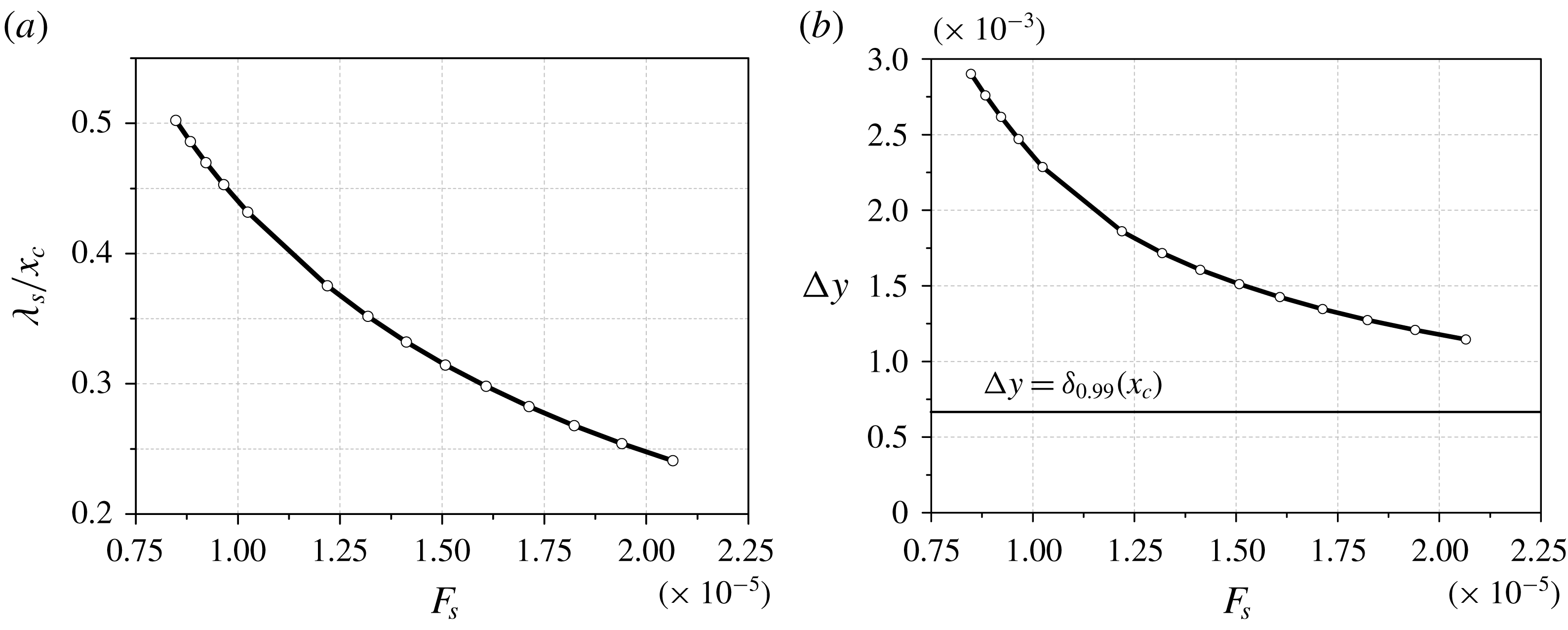
) the discrepancy is still substantial – the theory underestimates the hump amplitude by approximately 25 %. This discrepancy could be attributed to violation of the theoretical restriction
 $\unicode[STIX]{x1D706}_{s}/x_{c}\ll 1$
, where
 $\unicode[STIX]{x1D706}_{s}=2\unicode[STIX]{x03C0}/\unicode[STIX]{x1D6FC}_{TS,r}(\unicode[STIX]{x1D714}_{s},\unicode[STIX]{x1D6FD}_{s},x_{c})$
is the length of the dominant wave at the collision point. In this case, the first-mode eigenfunction
 $\hat{q}_{m}(x_{c},y,\unicode[STIX]{x1D6FD}_{s},\unicode[STIX]{x1D714}_{s})$
penetrates the outer inviscid flow for a large distance from the wall, as shown in figure 11(b). The penetration depth
 $\unicode[STIX]{x0394}y$
is estimated as
 $\unicode[STIX]{x0394}y=\unicode[STIX]{x1D705}_{r,min}^{-1}$
, where
 $\unicode[STIX]{x1D705}_{r,min}$
is the real part of the minimal damping rate of the eigenfunction vector proportional to
 $\text{e}^{-\unicode[STIX]{x1D705}y}$
in the outer flow. Figure 11(a) shows the ratio
 $\unicode[STIX]{x1D706}_{s}/x_{c}$
as a function of the frequency parameter
 $F_{s}=\unicode[STIX]{x1D714}_{s}^{\ast }\unicode[STIX]{x1D708}_{e}^{\ast }/U_{e}^{\ast 2}$
. For low frequencies corresponding to the far-field stations in figure 10, the ratio is not small:
 $\unicode[STIX]{x1D706}_{s}/x_{c}\approx 0.5$
. To check this argument, we performed computations for the doubled collision point
 $x_{c}=0.134$
. However, this did not reduce the discrepancy (see figure 10).
Theoretical (lines with white symbols) and numerical (black symbols) distributions of the hump amplitude
 $p_{w,max}^{\prime }(x_{max})$
for the collision points
 $x_{c}=0.067$
(circles) and
 $x_{c}=0.134$
(stars);
 $F_{s}$
– frequency parameter of the dominant wave at the observation point
 $x_{max}$
.

The ratio
 $\unicode[STIX]{x1D706}_{s}/x_{c}$
(a) and the penetration depth
 $\unicode[STIX]{x0394}y$
(b) as functions of frequency parameter
 $F_{s}$
.
Another reason could be the spectral content of the particle-induced disturbance. The NS disturbance contains all modes of the discrete and continuous spectra, while the theoretical solution (2.14)–(2.17) consists of the first mode only. To check this argument we performed spectral and normal-mode analyses of the NS disturbance in the case of
 $x_{c}=0.134$
. We considered the near-field station
 $x=0.2$
, which is located just downstream of the collision point, and the far-field station
 $x=0.6$
, where the amplification factor (2.17) is
 $N(x_{c},x)\approx 5$
. Figure 12 shows the spectral density modulus of the wall pressure disturbance computed using (2.18), where the spanwise wavenumber
 $\unicode[STIX]{x1D6FD}$
and frequency
 $\unicode[STIX]{x1D714}$
are made non-dimensional as:
 $\unicode[STIX]{x1D714}=\unicode[STIX]{x1D714}^{\ast }L^{\ast }/U_{\infty }^{\ast }$
;
 $\unicode[STIX]{x1D6FD}=\unicode[STIX]{x1D6FD}^{\ast }L^{\ast }$
. The Fourier transform (2.18) is evaluated using the discrete fast Fourier transform. The space and time samplings are chosen for the inverse transform to restore the original signal with the relative error less than 1 %. In the case of
 $x=0.2$
, the discretization versus time and spanwise coordinate has
 $N_{t}=250$
and
 $N_{z}=200$
points, respectively. At
 $x=0.6$
it is sufficient to have
 $N_{t}=100$
and
 $N_{z}=100$
. In the near-field station (figure 12
a) the NS disturbance has a broad spectrum of rather complex shape. As the disturbance propagates downstream, oblique waves of the first mode grow exponentially. Their selective amplification results in the wavepacket of the relatively simple spectrum shown in figure 12(b).
In order to confirm that the far-field disturbance is predominantly the first mode, we extract the first-mode wavepacket from the NS disturbance using the biorthogonal eigenfunction decomposition method outlined in § 2. Figure 13 compares the wall pressure fluctuations
 $p_{w}^{\prime }(t)$
at the near-field point
 $(x,z)=(0.2,0)$
and at the far-field point
 $(x,z)=(0.6,0)$
. The NS fluctuation is shown by the grey line (red online) while the first-mode fluctuation, which is computed using (2.21), is shown by the black line (blue online). It is seen that the NS disturbance quickly converges to the first-mode wavepacket. Therefore, the discrepancy between the numerical simulation and the theoretical prediction in figure 10 is not associated with the presence of other modes.
The spectral density modulus of the wall pressure disturbance at different stations. White circles denote the theoretical location of the dominant wave
 $(\unicode[STIX]{x1D6FD}_{s},\unicode[STIX]{x1D714}_{s})$
: (a)
 $x=0.2$
,
 $(\unicode[STIX]{x1D6FD}_{s},\unicode[STIX]{x1D714}_{s})=(584,121)$
; (b)
 $x=0.6$
,
 $(\unicode[STIX]{x1D6FD}_{s},\unicode[STIX]{x1D714}_{s})=(402,79.5)$
. The collision point is
 $x_{c}=0.134$
.

The wall pressure oscillograms at
 $(x,z)=(0.2,0)$
(a) and
 $(x,z)=(0.6,0)$
(b).

This discrepancy could be due to a low accuracy of the far-field asymptotic approximation (2.14) of the double integral (2.10). This approximation is based on the steepest descent method assuming that the selective amplification is strong while receptivity weakly depends on
 $\unicode[STIX]{x1D714}$
and
 $\unicode[STIX]{x1D6FD}$
. The corresponding mathematical restrictions are
 $$\begin{eqnarray}\displaystyle N(\unicode[STIX]{x1D714}_{s},\unicode[STIX]{x1D6FD}_{s})\gg 1,\quad \unicode[STIX]{x1D700}_{\unicode[STIX]{x1D6FD}}=\frac{\left|\displaystyle \frac{\unicode[STIX]{x2202}_{\unicode[STIX]{x1D6FD}}f(\unicode[STIX]{x1D714}_{s},\unicode[STIX]{x1D6FD}_{s})}{f(\unicode[STIX]{x1D714}_{s},\unicode[STIX]{x1D6FD}_{s})}\right|}{\unicode[STIX]{x1D6FD}_{s}|\unicode[STIX]{x2202}_{\unicode[STIX]{x1D6FD}\unicode[STIX]{x1D6FD}}^{2}N(\unicode[STIX]{x1D714}_{s},\unicode[STIX]{x1D6FD}_{s})|}\ll 1,\quad \unicode[STIX]{x1D700}_{\unicode[STIX]{x1D714}}=\frac{\left|\displaystyle \frac{\unicode[STIX]{x2202}_{\unicode[STIX]{x1D714}}f(\unicode[STIX]{x1D714}_{s},\unicode[STIX]{x1D6FD}_{s})}{f(\unicode[STIX]{x1D714}_{s},\unicode[STIX]{x1D6FD}_{s})}\right|}{\unicode[STIX]{x1D714}_{s}|\unicode[STIX]{x2202}_{\unicode[STIX]{x1D714}\unicode[STIX]{x1D714}}^{2}N(\unicode[STIX]{x1D714}_{s},\unicode[STIX]{x1D6FD}_{s})|}\ll 1,\qquad & & \displaystyle\end{eqnarray}$$
where
 $f(\unicode[STIX]{x1D714},\unicode[STIX]{x1D6FD})=D_{m}(\unicode[STIX]{x1D714},\unicode[STIX]{x1D6FD};x_{c})\hat{q}_{m}(x,y,\unicode[STIX]{x1D6FD},\unicode[STIX]{x1D714})$
in (2.10). As shown in figure 14, the parameters
 $\unicode[STIX]{x1D700}_{\unicode[STIX]{x1D714}}$
and
 $\unicode[STIX]{x1D700}_{\unicode[STIX]{x1D6FD}}$
decrease slowly with
 $x$
. In the cases presented in figure 10, they are not very small (
 $\unicode[STIX]{x1D700}_{\unicode[STIX]{x1D714}}\sim \unicode[STIX]{x1D700}_{\unicode[STIX]{x1D6FD}}\approx 10\,\%$
) and the
 $N$
-factor is not very large (
 $N<7.5$
). This concern is confirmed by the fact that the theoretical locus
 $(\unicode[STIX]{x1D6FD}_{s},\unicode[STIX]{x1D714}_{s})$
of the spectrum maximum, which is determined using (2.12), poorly correlates with the numerical data (see figure 12). Although the theoretical curves in figure 10 verge toward the numerical ones as the observation point
 $x_{max}$
moves downstream, the convergence is slow and the discrepancy remains appreciable by the end of the computational domain. A similar slow convergence is observed in comparisons of the wavepacket hump trajectories (figure 8) and the wave-front angles (figure 9).
Distributions of parameters
 $\unicode[STIX]{x1D700}_{\unicode[STIX]{x1D714}}$
,
 $\unicode[STIX]{x1D700}_{\unicode[STIX]{x1D6FD}}$
and
 $N$
-factors (2.17) versus the observation point
 $x$
.

The leading-order theoretical solution is indifferent to whether the particulate falls onto the surface or flies away after a perfectly elastic collision; i.e. the receptivity coefficient satisfies the condition
 $|C_{recept}(v_{p})|=|C_{recept}(-v_{p})|$
, where
 $v_{p}$
is the
 $y$
-component of the particulate velocity. To check this result we performed computations for the case where the particulate is launched from the wall point
 $y_{pw}=0,x_{pw}=x_{c}-\unicode[STIX]{x0394}x,z_{pw}=0$
with the initial velocity corresponding to the case of perfect reflection. Here
 $x_{c}=0.067$
and the upstream shift
 $\unicode[STIX]{x0394}x=\unicode[STIX]{x1D6FF}_{0.99}(x_{c})/\tan (14^{\circ })$
is for the particulate to interact with the same boundary-layer region as in the base case. It has been found that the deviation from the base case is small,
 $\unicode[STIX]{x0394}p_{w,max}^{\prime sym}\approx -4.3\,\%$
, in accord with the theoretical prediction. This opens up an opportunity to set up controlled experiments on receptivity to particulates. By shooting calibrated particulates from the wall and synchronizing measurements of boundary-layer disturbances with the particulate strikes one could determine the receptivity coefficient.
5 Summary
A numerical model has been developed to simulate excitation of unstable wavepackets by spherical solid particulates. Namely, the analytical solution (Fedorov Reference Fedorov2013) was replaced by numerical integration of the full Navier–Stokes equations with the particulate-induced source terms taken from the original analysis (Fedorov Reference Fedorov2013). To cross-validate the theoretical and numerical models, computations were performed for a test case: a
 $14^{\circ }$
half-angle sharp wedge flying at altitude 20 km at Mach number 4 and zero angle of attack. A spherical particulate of density
 $\unicode[STIX]{x1D70C}_{p}^{\ast }=10^{3}~\text{kg}~\text{m}^{-3}$
and radius
 $R_{p}^{\ast }=10~\unicode[STIX]{x03BC}\text{m}$
collides with the wedge surface at the streamwise distance of
 ${\approx}6.7~\text{cm}$
from the leading edge. The particulate excites a first-mode wavepacket propagating downstream and growing in space.
Using the in-house software HSFlow, it has been shown that the receptivity process is simulated with the error
 $\unicode[STIX]{x0394}p_{w,max}^{\prime sym}<1\,\%$
if:
(i) the particulate-induced point source is modelled by a Gaussian distribution of width
 $\unicode[STIX]{x1D70E}$
at which the characteristic diameter
$2\unicode[STIX]{x1D70E}\sqrt{2}$
is less than 22 % of the boundary-layer thickness at the collision station;
(ii) the grid resolves the source term with at least
$6\times 6\times 6$
points along the trajectory as well as in the collision region where the
$y$
-resolution becomes finer than the others. The error rises to approximately 3 % for coarser resolution of
$3\times 3\times 3$
points without using the symmetry assumption;(iii) the temporal resolution provides at least 25–30 time steps as the particulate crosses the boundary layer.


Comparisons of the theoretical and numerical solutions show:
(i) the wavepacket hump trajectory deviates from the centre line and slowly approaches the asymptotic trajectory predicted by the linear stability theory in the far-field region where the amplification factor of the dominant wave is
$N(x_{c},x)>4.9$
;(ii) in the far field, the theory underestimates the wavepacket hump amplitude by approximately 25 %. Presumably, this discrepancy is due to low accuracy of the far-field asymptotic approximation (2.14) of the double integral (2.10).

The numerical simulation confirmed the theoretical prediction that receptivity is almost indifferent to whether the particulate falls onto the surface or flies away after a perfectly elastic collision. This opens up an opportunity to set-up controlled experiments on receptivity. By shooting calibrated particulates from the wall and synchronizing measurements of boundary-layer disturbances with the particulate strikes one could determine the receptivity coefficient.
The developed numerical model can be used for simulations of receptivity to particulates for practical supersonic and hypersonic configurations such as blunt bodies of revolution. In particular, it is feasible to treat the interaction of particulates with strongly non-parallel flows near the body nose where the theoretical model is not valid.
Acknowledgements
This work is carried out in Moscow Institute of Physics and Technology (MIPT) under the financial support of Russian Science Foundation (RSF, Project no. 14-19-00821). Numerical simulations have been carried out using computing resources of the federal collective usage center Complex for Simulation and Data Processing for Mega-science Facilities at NRC ‘Kurchatov Institute’, http://ckp.nrcki.ru/; and HPC resources of MIPT (FlowModelliumLab).
Supplementary movie
Supplementary movie is available at https://doi.org/10.1017/jfm.2018.842.



