


1. Introduction
Emerging markets suffer from substantial macroeconomic instability, frequently associated with prolonged debt crises due to outright sovereign default. To resolve such episodes and regain good credit standing in international financial markets, the governments of these countries renegotiate their defaulted debt with their lenders. The negotiated terms specify a new level of debt, the recovery, that the country promises to pay as compensation to their creditors. This debt recovery is important because it affects not only the country’s debt burden and fiscal policy but also its future economic growth (see Forni et al. Reference Forni, Palomba, Pereira and Richmond2016; Reinhart and Trebesch Reference Reinhart and Trebesch2016).Footnote 1
Despite its importance for welfare, the determinants of recovery in renegotiation have not been well understood since most previous work focuses on creditors’ loss, measured by haircuts. This paper attempts to fill this gap by analyzing the role of outstanding debt levels for the eventual recovery in a quantitative framework for emerging market debt crises and their resolution. Standard models based on Nash bargaining suggest that past debt is a bygone once default has occurred: recovery is determined by the surplus generated by settlement and market re-entry, rather than by the face value of claims in default. This implication is often summarized as the “bygones are bygones” property of sovereign debt renegotiation.
The data suggest otherwise. Using emerging market data documented in Cruces and Trebesch (Reference Cruces and Trebesch2013), we find a strong positive relationship between defaulted debt and debt recovery. As shown in Figure 1, episodes with larger defaulted-debt-to-GDP ratios are associated with larger recovery-to-GDP ratios. This relationship is further supported by a series of regression analyses of recovery-to-GDP on defaulted-debt-to-GDP, controlling for macroeconomic conditions. The evidence suggests that the level of debt entering default is not merely a historical liability; it is systematically related to the amount eventually recovered in restructuring.
Debt and recovery.
Notes: (1) Each solid point represents a restructuring event. (2) Debt and recovery are measured in net present value. (3) GDP in both axes are measured at the year of exiting restructuring. (4) Out of the 171 events, this figure only shows 168 events whose defaulted debt to GDP ratio is below 0.5. The figure with full sample is included in Online Appendix A. (5) For both variables, GDP is in the year of exiting debt restructuring. Data source: Cruces and Trebesch (Reference Cruces and Trebesch2013), World Bank World Development Indicator (WDI).

To account for this new stylized fact, we develop a quantitative sovereign default model with debt renegotiation based on the Kalai-Smorodinsky bargaining solution. In the model, the risk-averse sovereign borrows internationally from the competitive and risk-neutral lenders, with an option to default and suspend payment. Default supports higher consumption but entails a temporary loss of market access and an output penalty. To regain good credit standing and re-enter financial markets, the sovereign must renegotiate the defaulted obligations with its lenders. This process determines the new debt payment for the country, the recovery received by the lenders, and thus the implied haircuts. We focus on the determinants of this recovery, in particular its response to the amount of defaulted debt and economic fundamentals. The renegotiation process is modeled with the cooperative bargaining solution of Kalai and Smorodinsky (Reference Kalai and Smorodinsky1975), and the results are compared with a standard bargaining protocol in Nash (Reference Nash1950).
By calibrating the model to the salient features of the emerging market data as documented in Neumeyer and Perri (Reference Neumeyer and Perri2005) and Cruces and Trebesch (Reference Cruces and Trebesch2013), we are able to replicate the recovery in renegotiation, jointly with the behavior of spreads and business cycle statistics. The numerical results show that the model matches well the correlation of debt recovery with defaulted debt, approximately
 $0.9$
in both the model and the data, together with a negative but more volatile correlation of the haircuts with GDP, of
 $-0.46$
. Moreover, it captures roughly three-quarters of the impact of defaulted debt on debt recovery in the data. The model is also successful in capturing the dynamics of recovery while preserving key desirable features in this class of models, namely the counter-cyclical spreads and trade balances, as well as the excess volatility of consumption relative to income, in line with emerging market data.
In the model, the level of debt at the time of default is a fundamental and key determinant of the eventual recovery received by creditors. This channel emerges naturally in the Kalai-Smorodinsky (K-S) axiomatic approach to bargaining, in which lenders evaluate proposals in reference to the best possible outcome for them, which is full recovery of defaulted debt. Their axiom of monotonicity captures the intuition that bargaining will compensate lenders more if there is more scope for recovery. We show that the quantitative success of the model is driven by this feature of the bargaining solution. In addition, the K-S bargaining solution reflects an “equal sacrifice” condition. This is a desirable property because many renegotiation events are coordinated by a third party, such as the IMF, who attempts to be impartial in the process (Panizza et al. Reference Panizza, Sturzenegger and Zettelmeyer2009). The aim of such institutions is to reach outcomes where both parties extend concessions in a balanced manner.
To identify the mechanism driving the recovery in the model and analyze its ability to replicate patterns in the data, we compare the results with a reference model that employs the more common Nash bargaining protocol, as studied by Yue (Reference Yue2010) and more recently by Asonuma and Trebesch (Reference Asonuma and Trebesch2016), Arellano et al. (Reference Arellano, Bai and Lizarazo2017), and Sunder-Plassmann (Reference Sunder-Plassmann2018). With Nash bargaining, Yue (Reference Yue2010) finds that debt at the time of default plays no role in determining recovered debt, a result labeled as “bygones are bygones.” This is because efficient Nash bargaining aims at maximizing the joint surplus created by recovery and market re-entry, a quantity inherently unrelated to past indebtedness. The lenders’ ability to prevent the sovereign from returning to markets is an all-or-nothing choice, independent of how much debt has defaulted. It is efficient for the country to resume borrowing, so the Nash solution finds a split of the surplus given their bargaining powers and the sovereign’s re-entry after renegotiation. The reference model with Nash bargaining, even when recalibrated, cannot match the strong positive relationship between recovery and defaulted debt. In the regression analysis using simulated data, the effect of defaulted debt on debt recovery is trivial in the Nash model, inconsistent with the large and significant magnitude in the data.
Finally, we study the welfare implications of debt relief programs conducted by a third party in the framework. Specifically, we study two programs: a loan program and a grant program in the form of debt buyback. Both programs aim to reduce the level of default debt in renegotiation. The programs benefit the defaulting country by lowering the level of debt recovery and hence the re-entry cost, a channel that is absent in the model with Nash bargaining. As the size of the default increases, the welfare gains become larger for the country, which supports the idea that a third party like the IMF should intervene in severe sovereign default events.
Related Literature Our model builds on the quantitative framework of sovereign default with incomplete markets and lack of commitment in Aguiar and Gopinath (Reference Aguiar and Gopinath2006), Arellano (Reference Arellano2008), and Chatterjee and Eyigungor (Reference Chatterjee and Eyigungor2012).Footnote 2 However, these papers mainly focus on business cycle statistics for emerging markets with defaults and do not consider recovery. Our model is most related to Yue (Reference Yue2010), which is one of the first quantitative debt recovery analyses. Her paper focuses on recovery rates using Nash bargaining in renegotiation, while this paper focuses on debt level using K-S bargaining.
Several recent papers on sovereign borrowing also consider recovery. For instance, Hatchondo et al. (Reference Hatchondo, Martinez and Sosa-Padilla2016) study recovery under long-term debt and its implications for the role of debt dilution. Asonuma (Reference Asonuma2016) studies “serial defaulter” behavior and its relation to recovery and spread premium. In Arellano et al. (Reference Arellano, Bai and Lizarazo2017), the presence of risk-averse lenders creates strategic complementarity in default decisions in emerging markets. Sunder-Plassmann (Reference Sunder-Plassmann2018) argues that variation in bargaining power over the business cycle is important in predicting the timing of defaults. Mihalache (Reference Mihalache2020) studies the role of maturity choice in light of the ubiquitous use of “maturity extensions” in renegotiation. Hatchondo et al. (Reference Hatchondo, Martinez and Sosa Padilla2014) and Asonuma and Trebesch (Reference Asonuma and Trebesch2016) discuss the distinct role of preemptive debt restructuring in data and models. Arellano and Bai (Reference Arellano and Bai2013) and (Reference Arellano and Bai2014) explain joint default and examine the role of policy when multiple countries borrow from and renegotiate with the same lenders. Azzimonti and Quadrini (Reference Azzimonti and Quadrini2024) study cross-country macroeconomic spillovers with renegotiations between countries after sovereign default. In contrast with these papers, we focus on the determination of the level of recovery and the limitations imposed by the standard Nash mechanism and provide a tractable alternative. Stefanidis (Reference Stefanidis2024) highlights the role of IMF lending in shaping the outcome of the renegotiation. In his model, the lending alters the outside option in the bargaining after default, while in our model the level of defaulted debt is the key in determining debt recovery.
Another strand of literature introduces a noncooperative bargaining process and has a main focus on explaining the long and costly duration of the renegotiation process and how the duration affects the final negotiation results. For instance, Bi (Reference Bi2008), Pitchford and Wright (Reference Pitchford and Wright2011), and Benjamin and Wright (Reference Benjamin and Wright2009) consider a mechanism that delivers market exclusion with endogenous length and find that delays are beneficial in that they allow both parties to access more resources when the debtor eventually recovers from a recession. Bai and Zhang (Reference Bai and Zhang2012) build a model with private information in the bargaining to explain the difference in negotiation duration between loans and bonds. Asonuma and Joo (Reference Asonuma and Joo2020) incorporate risk-averse creditors and find that when they experience high growth, renegotiations are prolonged and settled with smaller haircuts. Dvorkin et al. (Reference Dvorkin, Sánchez, Sapriza and Yurdagul2021) consider both debt payment and maturity in restructuring and can quantitatively mimic the patterns surrounding debt restructuring and business cycle properties. In contrast, we take the duration of exclusion as exogenously given and focus on the debt recovery levels.
Our paper also contributes to the salient empirical work. For instance, Cruces and Trebesch (Reference Cruces and Trebesch2013) assembles a comprehensive dataset including 187 debt restructuring events. Zettelmeyer et al. (Reference Zettelmeyer, Trebesch and Gulati2013) document cash flows and haircuts in the 2012 Greece default event and thus extend the dataset in Cruces and Trebesch (Reference Cruces and Trebesch2013). Asonuma and Trebesch (Reference Asonuma and Trebesch2016) complement the analysis of the Cruces and Trebesch (Reference Cruces and Trebesch2013) data by differentiating preemptive and post-default restructuring events. We are different in documenting a new stylized fact of the positive relationship between debt restructured and debt recovery using these data, motivating the choice of K-S bargaining in renegotiation.
The rest of the paper is organized as follows. Section 2 introduces empirical results from data that motivate the model. Section 3 discusses the model environment and describes its differences from a parallel model using Nash bargaining. Section 4 provides the model calibration and the results of quantitative analysis. Section 5 studies the welfare implications of debt relief programs. Section 6 concludes the paper.
2. Empirical motivation
We use a comprehensive dataset built by Cruces and Trebesch (Reference Cruces and Trebesch2013) to study the relationship of the sovereign debt restructuring and the sovereign country’s debt burden after renegotiation. Figure 1 contains the recovery events in the data set.Footnote 3 Each point represents one event, with the ratio of the defaulted debt to GDP on the horizontal axis and the eventual recovery-to-GDP ratio on the vertical axis. The recovery is defined by the present value of the new debt after restructuring.
There are two facts worthy to be pointed out in Figure 1. First, the recovered debt is always lower than the defaulted debt, as most of the points are below the dashed
 $45$
degree line.Footnote
4
Second and more importantly, there is a positive relationship between these two variables: When the level of defaulted debt is higher, the debt recovery after restructuring is also higher. To our best knowledge, we are the first to document this pattern.
We then conduct a series of regression analyses to further confirm this positive relationship. We combine the Cruces and Trebesch (Reference Cruces and Trebesch2013) dataset with another database of sovereign defaults built by Asonuma and Trebesch (Reference Asonuma and Trebesch2016) and update the combined dataset to 2020 to pin down the start and end years of each renegotiation episode. Then, we can extract the cyclical component of GDP and the duration of each default event. GDP data for the countries involved come from the World Bank WDI dataset.
Table 1 reports the benchmark regression results. The dependent variable is the debt recovery to GDP ratio. We scale both defaulted debt and recovery by GDP to make default and recovery outcomes comparable across countries and restructuring episodes. This normalization accounts for the fact that the same nominal amount of defaulted debt may imply very different repayment pressures depending on a country’s economic size and condition. In Table 1, both Recovery/GDP and Defaulted Debt/GDP are scaled by GDP in the exit year of restructuring.Footnote 5
Regression results

Table 1. Long description
A table with regression results for the dependent variable recovery/GDP. The table has five columns: Full sample (1), Full sample (2), Full sample (3), Subsample by share Share < 0.5 (4), and Subsample by share Share >= 0.5 (5). Row labels include Defaulted debt/GDP, Total debt/GDP, GDP cycle, Observations, and Adjusted R2. Each cell contains regression coefficients with standard errors in parentheses. Notable trends include significant coefficients for Defaulted debt/GDP and GDP cycle in most columns, with varying magnitudes across different samples. The table also notes specific conditions and measurements used in the regression analysis.
Notes: (1) Robust standard errors are in parentheses. (2) GDP cycle is measured as log-linearly detrended real GDP in the trough year before the renegotiation is settled. (3) Column 2 replaces defaulted debt with total PPG external debt owed to private creditors, measured in the year prior to restructuring. Column 3 includes both. (4) Columns 4 and 5 split the sample at a defaulted share of 0.5, defined as defaulted debt divided by PPG external debt held by private creditors in the year prior to restructuring. (5)
 $^{*}p\lt 0.1$
,
 $^{**}p\lt 0.05$
,
 $^{***}p\lt 0.01$
.
Column (1) regresses recovery on defaulted debt. The coefficient on defaulted debt is
 $0.484$
, significant at the 1% level, indicating that a one-percentage-point increase in the defaulted-debt-to-GDP ratio raises the recovery-to-GDP ratio by approximately
 $0.484$
%. We also control the GDP cycle as the literature documents that business cycles have a positive effect on renegotiation outcomes (e.g. Asonuma and Trebesch Reference Asonuma and Trebesch2016; Sunder-Plassmann Reference Sunder-Plassmann2018).Footnote
6
Consistently, the GDP cycle is positive and significant, confirming that renegotiations conducted in better economic conditions yield higher recovery.
Considering that many sovereign default episodes are partial in practice, as emphasized by Arellano et al. (Reference Arellano, Mateos-Planas and Ríos-Rull2023), Column (2) replaces defaulted debt with total outstanding debt, which is measured by total public and publicly guaranteed (PPG) external debt owed to private creditors from the World Bank International Debt Statistics. This allows us to examine whether total outstanding debt is also associated with recovery, beyond the actual amount in default. The variable is measured in the year prior to restructuring to avoid contamination from face-value reductions or other debt relief operations implemented during the restructuring process. The coefficient on total debt is
 $0.219$
and significant at the
 $1\%$
level, indicating that the positive relationship is not confined to the defaulted portion of debt.
Column (3) further includes both defaulted debt and total debt in the same specification. The coefficient on defaulted debt remains virtually unchanged, at
 $0.482$
and highly significant at the 1% level, while the coefficient on total debt is
 $0.014$
and statistically indistinguishable from zero. This suggests that, although total outstanding debt is positively associated with recovery when entered alone, the relationship is primarily driven by the portion of debt that actually enters default.
To further examine the distinction between partial and near-full default, we construct a defaulted share, defined as defaulted debt divided by total outstanding private-creditor debt. We then split the sample at a threshold of
 $50\%$
.Footnote
7
Columns (4) and (5) report the results. In Column (4), where the defaulted share is below
 $50\%$
, the coefficient on defaulted debt is
 $0.474$
. In column (5), where the defaulted share is at or above
 $50\%$
, where the default covers the majority of outstanding private-creditor debt, the coefficient rises to
 $0.539$
.
In order to interpret these empirical patterns, we need a theoretical model that describes the debt restructuring and renegotiation process, which is illustrated in the next section.
3. Model
This section introduces a quantitative sovereign default model with a debt renegotiation process. In order to allow the level of debt at the time of default to be a determinant of the eventual recovery received by creditors, we introduce the Kalai-Smorodinsky (K-S) axiomatic approach to bargaining, in which the solution is determined concerning the “best possible outcomes” for the sovereign and creditors, and the renegotiation process lasts for one period.
In the model, there are two types of agents: a risk-averse sovereign country and a continuum of competitive and risk-neutral international lenders. The sovereign country issues one-period, non-contingent debt, so markets are incomplete as in Eaton and Gersovitz (Reference Eaton and Gersovitz1981) and Arellano (Reference Arellano2008).Footnote 8 Lacking commitment, the government may decide to default, in which case it will be temporarily excluded from the financial markets and suffer an endowment penalty. The benefit of default comes from the suspension of debt service payments. Eventually, default events are resolved through renegotiations, resulting in a debt recovery level and renewed market access.
3.1. The Sovereign Country
The country’s objective is to maximize its expected lifetime utility. The instantaneous utility function
 $u$
satisfies standard assumptions. It is continuous, strictly increasing, and concave and satisfies the Inada conditions. Each period, the country faces the state variables
 $\left (b,y\right )\in \mathbb{B}\times \mathbb{Y}$
, where
 $b\gt 0$
, indicating the debt position, or
 $b\lt 0$
, indicating the asset position, inherited from the last period with support
 $\mathbb{B}$
, and
 $y$
is the endowment following an exogenous process, a Markov chain with support
 $\mathbb{Y}$
. The value of the country with market access
 $V$
reflects the country’s decision of whether to continue paying back the debt with an associated value
 $V^{\text{P}}$
, or to exert the default option and obtain a value
 $V^{\text{D}}$
. Formally,
 \begin{equation} V(b,y)=\underset {d\in \left \{ 0,1\right \} }{\max }\quad (1-d)V^{\text{P}}(b,y)+dV^{\text{D}}(b,y) \end{equation}
where
 $d$
is the default decision indicator. Specifically,
 $d=1$
means that the country defaults, while
 $d=0$
means repaying.
If the country continues to service its debt, it maintains market access and can choose the next period’s debt
 $b'$
and consumption
 $c$
. The value it achieves in this case is given byFootnote
9
 \begin{equation} \begin{aligned} V^{\text{P}}(b,y) & =\underset {c,b'}{\max }\quad u(c) + \beta \mathbb{E}_{y'|y} \left [ V(b',y') \right ] \\ \text{s.t.} & \quad c = y + q(b',y)b' - b \end{aligned} \end{equation}
where
 $q(b',y)$
is the endogenous bond price schedule faced by the sovereign. It reflects the terms of loans extended to the government by international lenders.
Instead, if the country decides to default, it suspends debt payments at the cost of market exclusion and endowment penalty
 $h(y)$
from the present period. Due to credit market exclusion, the country can only consume an amount
 $y-h(y)\gt 0$
. From the next period following the default decision, with probability
 $\mu$
, the country renegotiates debt repayments with lenders. This process takes one period and results in the resumption of debt service payments, market access, and recovery for the lenders. With probability
 $1-\mu$
, the country remains in the state of default. The value of default is thus given by
 \begin{equation} V^{\text{D}}(b,y) = u ( y-h(y) ) + \beta \mathbb{E}_{y'|y} [ \mu V^{\text{R}}(b,y')+(1-\mu )V^{\text{D}}(b,y') ] \end{equation}
where
 $V^{\text{R}}(b,y)$
is the value of the country in the renegotiation period, defined as
 \begin{equation} V^{\text{R}}(b,y) = u(y-h(y)-R(b,y))+\beta \mathbb{E}_{y'|y} [V(0,y') ] \end{equation}
Here,
 $R(b,y)$
represents the debt recovery determined by the bargaining protocol which will be illustrated in the next subsection, and is paid immediately after a settlement is reached. The sovereign then enters the next period with zero debt. Without debt renegotiation, the debt will be carried over at the defaulted level during the periods in market exclusion.
3.2. Renegotiation problem
We apply a cooperative bargaining solution in the renegotiation phase.Footnote 10 Specifically, we employ the K-S bargaining proposed by Kalai and Smorodinsky (Reference Kalai and Smorodinsky1975) to determine the solution. This application contrasts with the use of Nash bargaining in seminal papers on cooperative restructurings, such as Yue (Reference Yue2010).
The K-S solution involves a reference point which captures the maximal utility levels for participants. The axiom of monotonicity ensures that the solution will change when this reference point changes. When the reference is more favorable to one party, the bargaining solution will be more favorable, too. In the context of debt renegotiation after default, the reference point for creditors is positively related to a full repayment from the sovereign. When the level of defaulted debt rises, there is more scope for debt recovery, which will be captured by the K-S solution. As a consequence, the level of defaulted debt will affect debt recovery under the K-S bargaining. In contrast, the Nash solution is defined on the axiom of independence of irrelevant alternatives, which implies that the solution is independent of any reference point.
Kalai- S morodinsky B argaining S olution
To determine the bargaining outcomes, we need to first define the values of the sovereign and the creditors in the disagreement point, which characterizes the unfavorable outcome when the negotiation breaks down. The risk-neutral creditors would simply obtain zero repayments and zero value if there is no agreement. For the sovereign debtor, however, a failure of negotiation would result in a permanent financial autarky and an endowment penalty.Footnote 11 Formally, the country’s value in autarky is
 \begin{equation} V^{\text{aut}}(y) = u ( y-h(y)) + \beta \mathbb{E}_{y'|y} [ V^{\text{aut}}(y')] \end{equation}
The reference point depends on the maximal surplus for the sovereign and the creditors which reflect their best outcomes. The sovereign’s best outcome can be achieved when the debt recovery is zero, under which the sovereign’s value is
 \begin{equation} V_{m}^{\text{S}}(y) = u (y-h(y)) + \beta \mathbb{E}_{y'|y}[ V(0,y')] \end{equation}
If the negotiation fails, the value is simply the one in autarky
 $V^{\text{aut}}(y)$
. The sovereign’s maximal surplus, denoted
 $\Delta _{m}^{S}(y)$
, is then the difference between
 $V_{m}^{S}(y)$
and
 $V^{\text{aut}}(y)$
 \begin{equation} \Delta _{m}^{\text{S}}(y) = \beta \mathbb{E}_{y'|y} [ V(0,y')-V^{\text{aut}}(y')] \end{equation}
We assume that the creditors’ reference claim is
 $(1-\theta ) b$
, where
 $b$
is the total value of the defaulted debt and
 $\theta \lt 1$
is a parameter capturing the bargaining power of the country. Note that the best outcome for the creditors is to obtain full repayment
 $b$
(when
 $\theta =0$
), while the reference repayment is only a proportion of it. When
 $\theta$
is larger, the creditors’ reference is smaller, and the bargaining solution is less favorable to the creditors.Footnote
12
Given that the creditors would get zero value in disagreement, the maximal surplus for them is
 \begin{equation} \Delta _{m}^{\text{C}}(b)=(1-\theta ) b \end{equation}
Next, we need to define the surplus at any given level of debt recovery
 $x$
. The country pays
 $x$
immediately, so its value at this level is
 $u ( y-h(y)-x )+\beta \mathbb{E}_{y'|y} [V(0,y') ]$
following Equation (4). Instead, if the negotiation breaks down, its value at the disagreement point is given by Equation (5). Therefore, the country’s surplus
 $\Delta ^{\text{S}}(x,y)$
is
 \begin{equation} \Delta ^{\text{S}}(x,y) = u(y-h(y)-x)-u(y-h(y))+\beta \mathbb{E}_{y'|y}\left [V(0,y')-V^{\text{aut}}(y')\right ] \end{equation}
Correspondingly, the creditors’ surplus
 $\Delta ^{\text{C}}(x)$
at
 $x$
is given by
 \begin{equation} \Delta ^{\text{C}}(x) = x \end{equation}
The optimal level of debt recovery, denoted by
 $R(b,y)$
, solves the following problem
 \begin{equation} \begin{aligned} R(b,y) \; & = \; \underset {x \geq 0}{\mathrm{arg\,max}}\quad \frac {\Delta ^{\text{S}}(x,y)}{\Delta _{m}^{\text{S}}(y)} \\ \text{s.t.} \; & \quad \frac {\Delta ^{\text{S}}(x,y)}{\Delta _{m}^{\text{S}}(y)}=\frac {\Delta ^{\text{C}}(x)}{\Delta _{m}^{\text{C}}(b)},\quad \Delta ^{\text{S}}(x,y)\geq 0,\quad \Delta ^{\text{C}}(x)\geq 0 \end{aligned} \end{equation}
where
 $\Delta ^{\text{S}}(x,y)$
,
 $\Delta _{m}^{\text{S}}(y)$
,
 $\Delta ^{\text{C}}(x,y)$
, and
 $\Delta _{m}^{\text{C}}(y)$
are defined in Equations (7) to (10).
The K-S solution shows that debt recovery
 $R(b,y)$
should make the “relative gains” of the two parties equal and maximized. This relative gain is measured as the ratio of surplus given the recovery to maximal surplus. For the sovereign country, the ratio is
 $\frac {\Delta ^{S}(x,y)}{\Delta _{m}^{S}(y)}$
, while for creditors it is
 $\frac {x}{(1-\theta )b}$
. In other words, the sovereign and creditors, with their reference outcomes as their claims, have to make concessions to reach an agreement, and the solution produces an equal sacrifice for both of them.
Most importantly, this solution highlights the role of defaulted debt
 $b$
as a reference for creditors in determining the debt recovery. Creditors are concerned about their potential losses and consider the debt owed by the defaulting country. Consequently, a change in the level of defaulted debt will affect the subsequent debt restructuring.
Nash bargaining solution
It is helpful to understand the K-S solution by comparing it to the widely used Nash bargaining solution. The Nash solution is different in the sense that it is efficient and forward-looking. The solution does not involve any reference point and only maximizes the Nash product of the surplus. Formally,
 \begin{equation} \begin{aligned} R_{\text{Nash}}(y) \; & = \; \underset {x}{\mathrm{arg\,max}} \quad [\Delta ^{\text{S}}(x,y)]^{\theta }[\Delta ^{\text{C}}(x)]^{1-\theta } \\ \text{s.t.} \; & \quad \quad \Delta ^{\text{S}}(x,y)\geq 0,\quad \Delta ^{\text{C}}(x) \geq 0 \end{aligned} \end{equation}
where
 $\theta \in \left [0, 1 \right ]$
measures the bargaining power of the sovereign.Footnote
13
Here,
 $R_{\text{Nash}}(y)$
is the Nash solution of debt recovery, and it is a function only of the endowment
 $y$
.
3.3. Bond price
The international creditors in the model are competitive, risk-neutral, and able to borrow or lend freely in the capital markets at a constant risk-free rate
 $r$
. Therefore, their expected profit must be zero, and the bond price
 $q$
satisfies
 \begin{equation} q(b',y) = \frac {1}{1+r} \mathbb{E}_{y'|y} [ 1-d(b',y')+d(b',y')\gamma (b',y') ] \end{equation}
where
 $\gamma (b',y')$
is the expected recovery rate satisfying
 \begin{equation} \gamma (b',y') = \frac {1}{1+r} \mathbb{E}_{y''|y'} \left [\mu \frac {R(b',y'')}{b'}+(1-\mu )\gamma (b',y'') \right ] \end{equation}
Note that
 $\gamma$
measures the price of defaulted debt. As in other sovereign default models with renegotiations, the debt recovery will affect the bond price schedule. On one hand, given the same default decision
 $d(b,y)$
, the higher debt recovery will lead to a higher
 $\gamma$
and hence a higher bond price. On the other hand, the sovereign’s default decision will also change with recovery. In equilibrium, the net effect is quantitatively ambiguous.
3.4. Recursive equilibrium
Based on the agents’ problems and the renegotiation process, we can define the stationary recursive equilibrium as follows.
Definition 1. A recursive equilibrium consists of a set of functions: (
 $\mathrm{i}$
) the country’s value functions, including the value with market access
 $V(b,y)$
, the value in repayment
 $V^{\text{P}}(b,y)$
, the value in default
 $V^{\text{D}}(b,y)$
, the value in the period of renegotiation
 $V^{\text{R}}(b,y)$
and the value in autarky
 $V^{\text{aut}}(y)$
, (
 $\mathrm{ii}$
) policy functions, including debt holdings
 $b^{'}(b,y)$
and the default policy
 $d(b,y)$
, (
 $\mathrm{iii}$
) debt recovery
 $R(b,y)$
, (
 $\mathrm{iv}$
) the bond price schedule
 $q(b',y)$
and the expected recovery rate
 $\gamma (b,y)$
such that:
-
• Given the bond price
 $q(b',y)$
and the debt recovery
$R(b,y)$
, the value functions
$V(b,y)$
,
$V^{\text{P}}(b,y)$
,
$V^{\text{D}}(b,y)$
and
$V^{\text{R}}(b,y)$
satisfy (1), (2), (3) and (4); the debt holdings
$b^{'}(b,y)$
and the default policy
$d(b,y)$
solve problem (2) and (1), respectively,
-
• The value function
$V^{\text{aut}}(y)$
satisfies (5), -
• Given the value functions
$V(b,y)$
and
$V^{\text{aut}}(y)$
, the debt recovery
$R(b,y)$
solves renegotiation problem (11), -
• Given the debt recovery
$R(b,y)$
and the default policy
$d(b,y)$
, the bond price
$q(b',y)$
and the expected recovery rate
$\gamma (b,y)$
satisfy Equations (13) and (14).


3.5. Characterization
Characterization of bargaining solutions in diagrams.
Notes: These two diagrams demonstrate the determination of the solutions with the K-S and the Nash bargaining. Both are drawn for illustration and are not derived from the numerical results in the next section.

A key feature of this model is that debt recovery is increasing in the level of debt at the time of default, as illustrated in Figure 2. Here,
 $x$
and
 $b$
have the same meaning as in the model, where
 $x$
stands for debt recovery and
 $b$
for defaulted debt. The analysis below holds for any
 $\theta \lt 1$
. Without loss of generality, suppose that
 $\theta = 0$
in the K-S bargaining. Consider two levels of defaulted debt
 $b_{1}$
and
 $b_{2}$
, and assume that
 $b_{1}\lt b_{2}$
.
Figure 2a shows the K-S bargaining solutions under
 $b_{1}$
and
 $b_{2}$
at a fixed level of endowment
 $y$
. The downward-sloping curve is the surplus ratio of the sovereign at the level of debt recovery
 $x$
. This curve is concave due to the concavity of the utility function and is decreasing in
 $x$
because the surplus
 $\Delta ^{\text{S}}(x,y)$
is decreasing in
 $x$
. Intuitively, when debt recovery is larger, the country has to pay more to re-enter the markets, and the surplus will be smaller. The upward-sloping lines are the surplus ratios of the creditors under the debt levels
 $b_{1}$
and
 $b_{2}$
, respectively. Since the recovery is paid in the period of renegotiation, the creditors’ surplus ratio is exactly equal to the recovery rate when
 $\theta = 0$
, denoted by
 $\frac {x}{b_{1}}$
and
 $\frac {x}{b_{2}}$
. As
 $b_{1}\lt b_{2}$
, the line
 $\frac {x}{b_{2}}$
is flatter than
 $\frac {x}{b_{1}}$
.
From the bargaining problem (11), the K-S solution is determined at the intersection of the country’s surplus ratio curve and the creditors’ surplus ratio curve. The solutions are denoted
 $x^{*}(b_{1})$
and
 $x^{*}(b_{2})$
. It is obvious that
 $x^{*}(b_{1}) \lt x^{*}(b_{2})$
, which implies that the debt recovery is increasing in the level of defaulted debt. This property is the main driving force that produces a high correlation between debt recovery and defaulted debt in the numerical exercise. The following proposition formalizes the result.
Proposition 1.
The K-S recovery solution
 $R(b,y)$
, as defined in problem (11), is increasing in the level of debt
 $b$
.
Proof. See Appendix A.
This feature exhibits the key difference from the Nash bargaining solution, which is derived from maximizing the Nash product. The curve in Figure 2b represents the Nash product
 $\Delta ^{\text{S}}(x,y)^{\theta }x^{1-\theta }$
, in which
 $\theta$
measures the bargaining power of the sovereign.Footnote
14
The two different levels of defaulted debt,
 $b_{1}$
and
 $b_{2}$
, are also marked on the x-axis. Note that the Nash product is not affected by the level of defaulted debt. When it increases from
 $b_{1}$
to
 $b_{2}$
, the solution is fixed at point
 $x^{*}$
where the Nash product is maximized. Debt recovery is therefore independent of the defaulted debt level, consistent with the “bygones are bygones” property of the default model with Nash bargaining studied in Yue (Reference Yue2010).Footnote
15
4. Quantitative analysis
This section provides a quantitative analysis of the model. First, we set functional forms and calibrate the parameters. In addition to the benchmark model with the K-S bargaining solution, we also calibrate a reference model with Nash bargaining. Next, we discuss the equilibrium properties and the difference in the debt recovery determination of the two models. Then we present the simulation results and highlight their performance in matching the positive correlation between the debt recovery and the level of defaulted debt in the data. Finally, a robustness check is conducted to demonstrate the distinction between the two models in explaining the positive relationship.
4.1. Functional forms
We assume that the instant utility function takes the CRRA form
 \begin{equation} u(c)=\frac {c^{1-\sigma }}{1-\sigma } \end{equation}
where
 $\sigma$
is the parameter for risk aversion. Following Chatterjee and Eyigungor (Reference Chatterjee and Eyigungor2012), we assume that the penalty function
 $h(y)$
in temporary exclusion takes the form
 \begin{equation} h(y)=\max \{\lambda _{0}y+\lambda _{1}y^{2},0\} \end{equation}
where
 $\lambda _{0}$
is negative and
 $\lambda _{1}$
is positive. The asymmetric output loss in default extends the set of risky loans to generate substantial default risk in equilibrium, and the quadratic form can help capture the average and volatility of spreads in calibration.
The endowment
 $y$
follows an AR(1) process as in Arellano (Reference Arellano2008)
 \begin{equation} \log (y_{t})=\rho \log (y_{t-1})+\epsilon _{t},\quad \epsilon _{t}\sim \text{N}(0,\eta ^{2}) \end{equation}
where
 $\rho$
and
 $\eta$
measure the persistence and volatility of the output cycles.
4.2. Calibration
Table 2 shows the calibration results. The length of a model period is one quarter. We set the risk aversion at
 $\sigma =2$
, which is standard in the sovereign default literature. The risk-free interest rate
 $r$
is set to
 $0.01$
to match the average yield of 3-month US treasury bills. The probability of re-entry
 $\mu$
is assumed to be
 $0.108$
, which implies an exclusion duration of
 $2.31$
years as in Das et al. (Reference Das, Papaioannou and Trebesch2012) and Dvorkin et al. (Reference Dvorkin, Sánchez, Sapriza and Yurdagul2021), broadly in line with evidence on more recent restructuring events. The parameters in the endowment process are set as
 $\rho =0.945$
and
 $\eta =0.025$
following Arellano (Reference Arellano2008), in which the two parameters are calibrated to the linearly detrended quarterly Argentinian GDP from 1980Q1 to 2001Q4.
Calibration

Table 2. Long description
The table presents calibration results for various parameters in a model period of one quarter. It is divided into two main sections: Parameters taken from the literature and Calibrated jointly. The first section includes four rows with parameters such as risk aversion, risk-free rate, persistence of output, standard deviation of output, and re-entry probability, along with their respective targets like US T-bill rate, Argentina GDP, and exclusion duration. The second section compares calibration results under K-S and Nash bargaining, listing parameters like discount factor, output cost in default, spread standard deviation, and bargaining power, with their respective targets such as TB standard deviation, average spread, spread standard deviation, and average recovery rate. Each row provides specific values for these parameters and targets.
Notes: The length of a model period is one quarter. The parameters in the lower block are calibrated jointly to match the same targets, separately under the K-S and the Nash bargaining.
There are four parameters to internally calibrate in the K-S model: the parameters of the output penalty in temporary market exclusion
 $\lambda _{0}$
and
 $\lambda _{1}$
, the parameter in the creditors’ reference point as the sovereign’s bargaining power in renegotiation
 $\theta$
, and the subjective discount factor
 $\beta$
. These parameters are jointly calibrated to match four targets: an average recovery rate of
 $62$
%, an annual average spread of
 $2.8$
%, an annual spread standard deviation of
 $2.3$
%, and an annual trade balance standard deviation of
 $2.4$
%. The data on the average recovery rate are computed from all the renegotiation events documented in Cruces and Trebesch (Reference Cruces and Trebesch2013). The annual average spread data are equal to the average of the four emerging markets studied in Arellano and Ramanarayanan (Reference Arellano and Ramanarayanan2012). The standard deviations of spreads and trade balance are borrowed from Neumeyer and Perri (Reference Neumeyer and Perri2005) involving a set of emerging markets. For the Nash model, we have the same set of parameters to calibrate jointly, where
 $\theta$
also captures the country’s bargaining power but is defined in the Nash bargaining setting, and the same moments of target.
4.3. Numerical results
We begin by examining the policy functions in the K-S model, with particular attention to debt recovery and spreads. Figure 3 shows how debt recovery, in the left panel, and annualized spreads, in the right panel, vary with the level of defaulted debt under K-S bargaining. The curves are plotted for three endowment states: the black curve marked with crosses corresponds to the zero shock, the blue curve marked with circles corresponds to a positive shock equal to one-half standard deviation, and the red curve marked with diamonds corresponds to a negative shock of the same magnitude.
From the left panel, we observe that debt recovery rises with defaulted debt and is always less than it. For example, with no endowment shock, when the level of defaulted debt is
 $0.2$
, the recovery is roughly
 $0.12$
. When debt increases to
 $0.4$
, the recovery also increases to approximately
 $0.16$
. This positive correlation is not surprising because it is driven by the K-S bargaining protocol in which a positive relationship has been proved in Section 3.5.
In terms of the spread function, we focus on the region where borrowing is below
 $0.2$
, corresponding to
 $20$
% of the debt service to GDP in average years, which is sufficiently high in a short-term debt model. As the right panel shows, the bond spreads increase with the country’s borrowing, which is standard in the sovereign default literature. However, at different levels of shock, the slopes are different. When the shock is negative, the slope of the spread curve is considerably steeper. As borrowing increases from
 $0.05$
to
 $0.1$
, the spreads increase rapidly from zero to approximately
 $5.4$
%. In contrast, given a zero shock, the spreads increase by less than
 $0.4$
%. In other words, they are more sensitive to debt changes following negative shocks.
Recovery and spreads on defaulted debt: K-S.
Notes: Policy function against defaulted debt for recovery (left) and spreads (right) of the calibrated K-S model. The blue line with circles is an endowment one half of a standard deviation above the mean, the black line with crosses is the mean, and the red line with diamonds is one half of a standard deviation below.

Recovery and spreads on endowments: K-S.
Notes: Policy functions against endowments for recovery (left) and spreads (right) of the calibrated K-S model. The blue line with circles is defaulted debt one half of a standard deviation above its simulated mean, the black line with crosses is the mean, and the red line with diamonds is one half of a standard deviation below.

The responses of debt recovery and spreads to endowment shocks are shown in Figure 4. The three curves represent three levels of debt where the mean level (black curve marked with
 $\times$
) is the mean debt value in the simulation, which equals
 $0.17$
or
 $17$
% of debt service to average year GDP. In the left panel, debt recovery is increasing with endowment shock at different levels of defaulted debt, a result consistent with the literature on sovereign debt restructuring, such as Yue (Reference Yue2010). The right panel exhibits that spreads increase during recessions. Here, the range of the x-axis is below and above half a standard deviation of the endowment process. It also shows that spreads inflate more drastically in deeper recessions and at higher levels of debt. These results are consistent with standard sovereign default models.
Policy functions: K-S and Nash.
Notes: The solid blue lines represent the K-S model and the dashed red lines the Nash model, each at its own calibration. The left panels fix the endowment at its mean; the right ones fix debt at the simulated mean of each model.

Figure 5 highlights the comparison between the K-S and Nash models. The blue solid curves are computed from the K-S model, and the red dashed curves are from the Nash model. The left panels plot the policy functions against debt, holding the endowment shock at zero; the right panels plot them against the endowment shock, holding debt at its simulated average level. The first row compares the debt recovery function. In the K-S model, debt recovery increases with the level of defaulted debt, while in the Nash model, it is independent of debt. This is the key distinction between the two bargaining protocols, which drives the difference in the simulation results and policy implications in the subsequent simulation results. In both models, the debt recovery function increases with the endowment shock, although the response is steeper in the Nash model because endowment is the only state variable affecting recovery. As a result, recovery is higher under K-S bargaining in bad times, while it is higher under Nash bargaining in good times.
The middle row reports the spread schedules. In both models, spreads increase with borrowing and decline with more favorable endowment shocks. However, the Nash model generally generates higher and steeper spreads.Footnote
16
This difference reflects the combined effects of debt recovery and default probabilities. When debt is below
 $0.1$
, the default probability is small, less than
 $1$
%, as shown in the left panel of the bottom row. In this region, debt recovery is less important given the small probability of default, and the spreads mainly reflect the difference in the default probability of the two models. When the level of debt increases from
 $0.1$
to
 $0.2$
, default probability increases and the potential recovery after default matters. Although the variation in default probability is small in the two models, the recovery on defaulted debt evolves differently. As the debt recovery is positively related to the level of defaulted debt under K-S bargaining, creditors expect fewer losses from the default; therefore, the spreads are considerably lower after taking into account the different default probabilities. The same logic explains the differences in the responses of spreads to endowment shocks.
4.4. Simulation results
Given the policy functions and the endowment process, we conduct a simulation for
 $100,000$
periods and remove the first
 $10,000$
periods to compute model statistics. The same statistics are computed for both the K-S model and the Nash model and are compared with the data. Data on business cycle moments come from Neumeyer and Perri (Reference Neumeyer and Perri2005). The trade balance is defined as a percentage of GDP, and output is log-linearly detrended GDP. Data on debt recovery and defaulted debt are from Cruces and Trebesch (Reference Cruces and Trebesch2013). The results are summarized in Table 3.
Model statistics

Table 3. Long description
A table comparing model statistics across different moments and data sources. The table has 15 rows and 4 columns. The columns are labeled Moments, Data, K-S, and Nash. The rows are grouped into four categories: Targeted, Business cycle, Default, and Recovery. Each row lists specific statistics and their values for the Data, K-S model, and Nash model. For example, under Targeted, the Avg. recovery rate is 62 percent for all three columns. Under Business cycle, the Consumption std./output std. is 1.3 for Data, 1.5 for K-S, and 1.5 for Nash. The Default category includes statistics like Avg. defaulted debt/output, which is 13 percent for Data, 4.3 percent for K-S, and 4.2 percent for Nash. The Recovery category lists correlations such as Corr(recovery, debt), which is 0.92 for Data, 0.89 for K-S, and 0.43 for Nash.
Notes: Business cycle moments are employed from Neumeyer and Perri (Reference Neumeyer and Perri2005); moments for debt default and recovery are calculated from the data in Cruces and Trebesch (Reference Cruces and Trebesch2013). The
 $1.7\%$
default probability is computed from Meyer et al. (Reference Meyer, Reinhart and Trebesch2019) in which 313 sovereign default episodes are documented for 91 countries between 1815 and 2016, implying a default probability equal to
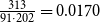 $\frac {313}{91 \cdot 202} = 0.0170$
.
The two models match quite well to the four targets of the moments. Regarding the business cycle statistics that are not calibrated to, both models induce the relative volatility of consumption to output of
 $1.5$
, which is slightly higher than
 $1.3$
in the data. The models successfully generate a countercyclical movement of spreads and trade balance, although the magnitude is smaller than that in the data, and a positive correlation between spreads and trade balance.
We also compute the mean and standard deviation of the defaulted-debt-to-GDP ratio. The mean from the K-S model is approximately
 $4.3$
%, which is similar in the Nash model at
 $4.2$
%. The volatilities are also similar at
 $1.3$
% in both models. The data value of
 $13$
% is the event-level mean of the face value of defaulted external debt owed to private creditors, scaled by GDP in the exit year of restructuring; it is not a measure of total sovereign debt to GDP. The model values are lower because the models feature one-period debt, while most of the restructured debt in the data is long-term. The model-implied values are best interpreted as debt-service obligations relative to GDP.Footnote
17
The default probability is
 $1.4$
% in the K-S model and
 $1.5$
% in the Nash model, both close to the value in the data.
Debt and recovery: data and simulation.
Notes: Black points are the restructuring events from the data set in Cruces and Trebesch (Reference Cruces and Trebesch2013) and red points are events simulated from each calibrated model; the blue dashed line is the
 $45$
degree line.

In the data, there is a highly positive relationship between debt recovery and restructured debt with a correlation of
 $0.92$
. This is well captured in the K-S model, which delivers a correlation of
 $0.89$
. This result is driven by the property of the K-S bargaining solution. The correlation of debt recovery with the output ratio and debt restructured with the output ratio is also very high in the data, which is
 $0.8$
. In the K-S model, the correlation is
 $0.89$
, while in the Nash model, it is only
 $0.33$
. Note that the correlations in the Nash model are still positive and relatively large even though the model implies that they should be independent. We can show that this is spurious, due to the length of market exclusion. A robustness check explores this feature of the Nash results later in the paper, in Section 4.6.
In the data, the correlation between the recovery-to-output ratio and output is only
 $0.02$
, which implies that the countries’ debt burden after renegotiation is not related to the cycles. Both models fail to capture this fact and show a strong positive relationship between the two variables.Footnote
18
Nonetheless, they perform well in having a positive correlation between haircuts and the defaulted-debt-to-output ratio as in the data. Haircuts are also countercyclical in the two models. The correlation in the K-S model is
 $-0.46$
. In summary, the models, especially the K-S model, fit well with the data.
To highlight the difference in the correlation between recovery and defaulted debt, we compare simulated data from the two models, which are represented by the semitransparent red points, and the data in Figure 6. The solid dark points represent restructuring events from the dataset in Cruces and Trebesch (Reference Cruces and Trebesch2013). The horizontal axis and vertical axis are exactly the same as in Figure 1, although the scales are zoomed in since the variation in the level of defaulted debt is smaller in the simulated data. Both subplots include all the simulated data and
 $97$
data events from Figure 1. The blue dashed lines are the 45-degree line. As shown in Figure 6a, the K-S model can generate a clear positive relationship between debt recovery and defaulted debt, which is close to the data, although less scattered. It exhibits linearity and a slope that is less than
 $1$
, which implies that when the level of defaulted debt increases by one percent, the recovery will increase by less than one percent. The simulation from the Nash model, as shown in Figure 6b, however, does not show any pattern, which means that debt recovery is independent of debt restructured.
Finally, we apply the regression analysis as in Section 2 to the simulated data from the two models. There are
 $1,121$
and
 $1,154$
debt restructuring events in the simulation of the K-S model and Nash model, respectively. To make them comparable with the data, we use the bootstrap method to obtain the coefficients. For each model, we randomly select the same number of simulated events as in the data and estimate for each draw. We perform
 $100$
draws and take the average of the coefficients and standard errors from every regression.
Table 4 reports the comparison between the data and the models. The dependent variable is the debt-recovery-to-GDP ratio, and the two regressors are the defaulted-debt-to-GDP ratio and the cyclical component of output. The simulated endowment sequence is log-linearly detrended in the same way as for the data. The Data column is copied from Column (1) in Table 1. Column (2) shows that the coefficient of debt recovery on defaulted debt is equal to
 $0.35$
and significant in the K-S model, compared to
 $0.48$
in the data regression. This means that the K-S model is able to explain approximately three-fourths of the positive effect of debt on recovery. In contrast, the value of the coefficient in Column (3) is essentially
 $0$
, indicating that defaulted debt has no significant impact on debt recovery in the Nash model. Therefore, the model with K-S bargaining performs better in capturing the positive relationship between debt recovery and debt restructured in the data.
Regression results: data and simulation

Table 4. Long description
The table presents a comparison of debt recovery to GDP using different models. It has four rows and three columns. The columns are labeled as Data, K-S, and Nash. The rows are labeled as Defaulted debt to GDP, GDP cycle, Observations, and Adjusted R squared. Row 1: Defaulted debt to GDP, Data: 0.48, K-S: 0.35, Nash: 0.00. Row 2: GDP cycle, Data: 0.13, K-S: 0.04, Nash: 0.11. Row 3: Observations, Data: 171, K-S: 171, Nash: 171. Row 4: Adjusted R squared, Data: 0.73, K-S: 0.94, Nash: 0.95. The table shows the coefficients and their significance levels for different models in explaining the debt recovery to GDP ratio.
Notes: (1) Robust standard errors in parentheses. (2) GDP cycle is measured as log-linearly detrended real GDP in the trough year during renegotiation for the data column, and is the one in the period of renegotiation in the K-S model and in the Nash model. (3) Debt is the value of restructured debt in Cruces and Trebesch (Reference Cruces and Trebesch2013), and is the level of defaulted debt in the two models. (4)
 $^{*}p\lt 0.1$
,
 $^{**}p\lt 0.05$
,
 $^{***}p\lt 0.01$
.
4.5. Additional testable predictions
The K-S bargaining model has two further testable implications beyond the positive relationship between recovery levels and defaulted debt. First, because the K-S policy function implies that recovery rises less than one-for-one with defaulted debt, the recovery rate—defined as recovery divided by the face value of defaulted debt—should decline as the size of default increases. Second, the recovery schedule should be increasing but concave in defaulted debt.
Taken together, the results support the two additional implications of the K-S bargaining model: larger defaults are associated with lower recovery rates, and the recovery schedule is increasing but concave in defaulted debt.
Table 5 examines these predictions and provides supportive evidence. Columns (1) and (2) regress the recovery rate on the defaulted-debt-to-GDP ratio. In Column (1), the coefficient is
 $-0.345$
and significant at the 1% level. Column (2) adds the GDP cycle to control for macroeconomic conditions at the time of restructuring. The coefficient on defaulted debt remains negative, while falling in magnitude to
 $-0.182$
, although it is no longer statistically significant at conventional levels (
 $p = 0.103$
). The coefficient on the GDP cycle is positive and significant, suggesting that recovery rates are higher when restructurings are concluded under more favorable economic conditions.
Recovery rates and recovery-schedule shape

Table 5. Long description
A table with three columns and five rows of data, plus additional notes. The table examines the relationship between recovery rates, defaulted debt to GDP ratio, and GDP cycle. Column headers are Recovery rate, Recovery/GDP (1), (2), (3). Row labels include Defaulted debt/GDP, GDP cycle, (Defaulted debt/GDP) squared, Observations, and Adjusted R-squared. Column (1) shows Defaulted debt/GDP with a value of -0.345***, GDP cycle with a value of 0.429***, Observations with a value of 173, and Adjusted R-squared with a value of 0.027. Column (2) shows Defaulted debt/GDP with a value of -0.182, GDP cycle with a value of 0.133***, Observations with a value of 171, and Adjusted R-squared with a value of 0.114. Column (3) shows Defaulted debt/GDP with a value of 0.711***, (Defaulted debt/GDP) squared with a value of -0.334***, Observations with a value of 171, and Adjusted R-squared with a value of 0.777. The table includes notes explaining the methodology and variables used in the regression analysis.
Notes: (1) Robust standard errors are in parentheses. (2) The dependent variable in Columns 1 and 2 is the recovery rate, defined as the restructured debt value divided by the face value of defaulted debt. (3) Column 3 augments the baseline specification from Column 1 of Table 1 with a quadratic term in the defaulted-debt-to-GDP ratio; the dependent variable is Recovery / GDP. (4) GDP cycle is log-linearly detrended real GDP in the trough year before the renegotiation is settled. (5)
 $^{*}p\lt 0.1$
,
 $^{**}p\lt 0.05$
,
 $^{***}p\lt 0.01$
.
Column (3) turns to the shape of the recovery schedule by using Recovery/GDP as the dependent variable and adding a quadratic term in the defaulted-debt-to-GDP ratio. The linear coefficient is positive at
 $0.711$
, while the quadratic coefficient is negative at
 $-0.334$
; both are significant at the 1% level. This pattern implies that recovery increases with defaulted debt but at a decreasing rate. The high adjusted
 $R^2$
of
 $0.777$
further indicates that the quadratic specification captures a substantial part of the variation in recovery outcomes.
4.6. Robustness check
The summary statistics in Table 3 show that under the calibrated parameters, the correlation between recovery and debt is
 $0.43$
in the Nash model, which contradicts the theoretical prediction of zero correlation. This positive correlation is mainly driven by the selection of periods in exclusion. In the calibration, we have a relatively high re-entry probability of
 $0.108$
, which implies a short market exclusion of
 $2.31$
years. As the debt recovery and the defaulted debt are both positively correlated with output and that output cannot fully revert to the average in such a short time before renegotiation, debt recovery and defaulted debt will be positively related. This correlation is not produced by the bargaining itself.
To confirm this intuition, we compute the correlation between recovery and debt using different values of
 $\mu$
with the value of other parameters being fixed. Table 6 documents the results for
 $\mu$
between
 $0.5$
and
 $0.017$
, which correspond to the average years in exclusion between
 $0.5$
and about
 $15$
years. The value in Column (4) is used in the calibrated models. It shows that as the duration of exclusion increases, the correlation decreases. When the average years in exclusion rises to about
 $15$
years, the correlation falls to
 $0.15$
in the Nash model, while in the K-S model, it also decreases but remains high at
 $0.62$
. Therefore, it is the value of
 $\mu$
that contributes to the high correlation in the calibrated Nash model.
Robustness check

Table 6. Long description
The table has 8 columns and 7 rows, including headers and notes. The columns are labeled (1) to (8) with values of 0.5, 0.25, 0.125, 0.108, 0.083, 0.042, 0.025, and 0.017. The rows are labeled with mu, Years, Cor(R,b) for K-S and Nash models, and Coefficient for K-S and Nash models. The Years row shows the corresponding average years in exclusion to the parameter. The Coefficient rows show the coefficients of recovery to GDP ratio to defaulted debt to GDP ratio in the regressions using simulated data from K-S and Nash models. The table notes provide additional context and robust standard errors in parentheses. Notable trends include a decrease in correlation as the duration of exclusion increases, with the K-S model maintaining a higher correlation compared to the Nash model.
Notes: (1) The Years row shows the corresponding average years in exclusion to the parameter
 $\mu$
. (2) The Coefficient rows show the coefficients of recovery to GDP ratio to defaulted debt to GDP ratio in the regressions as in Table 4 using simulated data from K-S and Nash models. (3) Column 4 in boldface indicates the results from the baseline model calibration, while the remaining columns present the model sensitivity to the Re-entry probability. (4) Robust standard errors in parentheses. (5)
 $^{*}p\lt 0.1$
,
 $^{**}p\lt 0.05$
,
 $^{***}p\lt 0.01.$
The length of market exclusion is also important in determining the effect of defaulted debt on debt recovery. On the one hand, longer exclusion means a higher cost of default, which will affect the country’s borrowing decision and the level of debt in default. On the other hand, the length of exclusion affects the realization of the endowment shock and its correlation with debt in the period of renegotiation, a factor that is relevant to the magnitude of debt’s effect in recovery. As parameter
 $\mu$
captures the average number of periods in market exclusion, we compute the coefficient on Defaulted Debt / GDP in Table 4 for the K-S and Nash models with different values of
 $\mu$
to check its role in determining the effect of debt on recovery. The results are also documented in Table 6.
In the K-S model, the coefficients are significantly positive and decreasing with the average years in exclusion. The reason is that when
 $\mu$
decreases, the country has to wait for a longer time to re-enter the financial markets. This change makes default more costly but also allows the country to hold more debt in equilibrium and induces a higher level of debt in default. As demonstrated in Figure 3, the marginal effect on recovery decreases with the level of defaulted debt. Therefore, a smaller
 $\mu$
drives up the debt level and weakens its impact on recovery, reflected in the coefficients. In the Nash model, the coefficients are insignificant and are close to zero. This result is consistent with the model prediction that the level of defaulted debt has a trivial effect on debt recovery.
Sensitivity Analysis: Bargaining Parameter The parameter
 $\theta$
governs the relative bargaining power of the debtor in renegotiation and enters the K-S problem through the creditor reference claim,
 $\Delta _m^C(b) = (1-\theta )b$
. Because
 $\theta$
directly determines the recovery payment in default, it has a first-order effect on the average recovery rate—the central target moment of the calibration. To assess whether the baseline results are robust to this parameter, Table 7 reports key model statistics under five values of
 $\theta$
spanning different magnitudes:
 $0.001$
,
 $0.01$
,
 $0.10$
,
 $0.50$
, and
 $0.90$
, holding all other parameters fixed at their calibrated values (
 $\beta = 0.929$
,
 $\lambda _0 = -0.241$
,
 $\lambda _1 = 0.259$
).
Sensitivity to the K-S bargaining parameter
 $\theta$

Table 7. Long description
The table presents a sensitivity analysis of key model statistics under five different values of the K-S bargaining parameter, with all other parameters held fixed at their calibrated values. The table has 12 rows and 6 columns. The columns are labeled with different values of the bargaining parameter: 0.001, 0.01, 0.1, 0.5, and 0.9. The rows are grouped into four main categories: Targeted, Business cycle, Default, and Recovery. Each row within these categories lists specific statistics. Row 1: Avg. recovery rate (%), with values 62, 61, 58, 41, 10. Row 2: Avg. spread (%), with values 2.8, 2.8, 2.9, 3.4, 3.4. Row 3: Spread std. dev. (%), with values 2.3, 2.4, 2.4, 2.6, 2.4. Row 4: Trade balance std. dev. (%), with values 2.4, 2.4, 2.4, 2.1, 1.7. Row 5: Consumption std./output std., with values 1.5, 1.5, 1.5, 1.4, 1.3. Row 6: Corr(trade balance, output), with values -0.45, -0.45, -0.44, -0.43, -0.39. Row 7: Corr(spreads, output), with values -0.47, -0.47, -0.49, -0.46, -0.41. Row 8: Corr(spreads, trade balance), with values 0.80, 0.80, 0.80, 0.78, 0.72. Row 9: Avg. debt/output (%), with values 4.3, 4.3, 4.0, 3.0, 2.1. Row 10: Std. debt/output (%), with values 1.3, 1.3, 1.3, 1.1, 0.9. Row 11: Default prob. (%), with values 1.4, 1.4, 1.4, 1.2, 0.8. Row 12: Corr(recovery, debt), with values 0.89, 0.91, 0.93, 0.97, 0.99. Row 13: Corr(recovery/output, debt/output), with values 0.89, 0.90, 0.92, 0.97, 0.99. Row 14: Corr(recovery/output, output), with values 0.62, 0.64, 0.63, 0.45, 0.39. Row 15: Corr(haircut, debt/output), with values 0.70, 0.70, 0.69, 0.71, 0.24. Row 16: Corr(haircut, output), with values -0.46, -0.42, -0.39, -0.36, -0.02.
Notes: (1) The column 1 in boldface indicates the baseline calibration (
 $\theta = 0.001$
), while the remaining columns present the model sensitivity to the bargaining power. (2) All the other parameters are held fixed at their calibrated values (
 $\beta = 0.929$
,
 $\lambda _0 = -0.241$
,
 $\lambda _1 = 0.259$
).
The results show that the main quantitative conclusions are robust across this range. As debtor bargaining strength increases, the creditor reference claim falls, lowering recovery: the average recovery rate declines from
 $62$
% at
 $\theta = 0.001$
to
 $10$
% at
 $\theta = 0.90$
, and average spreads rise from
 $2.8$
to
 $3.4$
% as creditors anticipate lower recovery ex ante. The recovery-related correlations are more sensitive to
 $\theta$
than are the business-cycle moments: the correlation between recovery and debt rises monotonically from
 $0.89$
to
 $0.99$
across the range, confirming that the positive recovery–debt relationship is a structural feature of the K-S bargaining mechanism. By contrast, default probabilities, the trade-balance volatility, and the standard business-cycle correlations remain virtually unchanged, indicating that the model’s cyclical implications are not driven by the specific value of
 $\theta$
.
5. Policy analysis
The costs and benefits of debt relief programs proposed by public institutions are important questions in the recent sovereign default literature (e.g. Arellano et al. Reference Arellano, Bai and Mihalache2024, Dvorkin et al. Reference Dvorkin, Sánchez, Sapriza and Yurdagul2021, Hatchondo et al. Reference Hatchondo, Martinez and Sosa-Padilla2020). In our settings with K-S bargaining, the level of debt is crucial in determining the renegotiation outcome. A debt relief program that reduces the level of defaulted debt prior to renegotiation will affect the recovery and the defaulting country’s welfare. This is a new channel that is absent in the reference model with Nash bargaining, whose solution is independent of the level of debt. Therefore, employing the K-S model will result in a substantially different program evaluation. In this section, we consider two debt relief programs, a loan program and a grant program, that are similar to those in Bulow et al. (Reference Bulow, Rogoff and Dornbusch1988) and Arellano et al. (Reference Arellano, Bai and Mihalache2024) to quantitatively study the impact of an unexpected reduction in the level of defaulted debt on the welfare changes of the country and the lenders in the K-S model and compare it with the results from the Nash model. Both programs demonstrate the distinct welfare implications between the two models, which highlights the essential role of debt restructuring in policy evaluation.
5.1. A loan program
We model a loan program by introducing a financial assistance entity (e.g., the IMF) that extends a default-free loan of fixed size to the country, which is similar to the one in Arellano et al. (Reference Arellano, Bai and Mihalache2024). The sovereign unexpectedly gets
 $L$
as a lump sum in the default period and begins to repay
 $l$
each period in perpetuity from now on.Footnote
19
The financial assistance entity discounts the future at the international rate
 $r$
and breaks even, so that the terms of the loan satisfy
 $l=\frac {r}{1+r}L$
.
The country uses the loan to retire a portion of the outstanding defaulted debt so that the remaining level of defaulted debt is
 $b^{\text{after}} = b-L$
. We evaluate the effects of a loan size of
 $2\%$
of the country’s output
 $y$
in the period of default.Footnote
20
Note that the loan program will make a difference under the K-S bargaining protocol because the reference point of the lenders changes from
 $b$
to
 $b^{\text{after}}$
. Therefore, it will affect the level of debt recovery and the welfare of the country and the lenders. In contrast, the Nash bargaining solution is independent of the defaulted debt, so the welfare change will also be constant across different values of defaulted debt. The complete model with the loan program is presented in Appendix B.
Welfare gains and losses are expressed relative to the baseline economy in present value. Specifically, the change in the welfare of the country is given by
 \begin{equation} \text{welfare change of the country} = \frac {\text{CE}^{\text{program}}}{1-\beta }-\frac {\text{CE}}{1-\beta } \end{equation}
where
 $\text{CE}$
is the consumption equivalence welfare without any program given by
 \begin{equation} \text{CE} = [(1-\beta )(1-\sigma )V^{\mathrm{D}}(b,y)]^{\frac {1}{1-\sigma }} \end{equation}
and
 $\text{CE}^{\text{program}}$
is the consumption equivalence welfare after receiving the loan
 \begin{equation} \text{CE}^{\text{program}} = [(1-\beta )(1-\sigma )V^{\mathrm{D,IMF}}(b,y)]^{\frac {1}{1-\sigma }} \end{equation}
For lenders, the welfare change can be expressed as
 \begin{equation} \text{welfare change of the lenders} = L + \gamma ^{\text{IMF}}(b, y, L) b^{\text{after}} - \gamma (b,y) b \end{equation}
where
 $\gamma ^{\text{IMF}}$
is the expected recovery in default after the intervention of the loan program, which is defined in (B.15) in Appendix B.
We evaluate the welfare change across quantiles of the default-time debt distribution, holding the endowment fixed at its median value in default for the K-S and the Nash model. The numerical results are reported in Table 8.
Welfare change (%) with the loan program

Table 8. Long description
A table comparing welfare change percentages across quantiles for K-S and Nash models. The table has 10 columns and 8 rows, including headers and row labels. Columns are labeled with quantiles ranging from 0.10 to 0.90. Rows are labeled as country, lenders, entity, and total for both K-S and Nash models. Row 1: K-S country, -4.19, -4.14, -4.14, -4.10, -4.07, -3.97, -3.95, -3.84, -3.65. Row 2: K-S lenders, 0.54, 0.56, 0.54, 0.55, 0.49, 0.46, 0.41, 0.30, 0.14. Row 3: K-S entity, 0.00, 0.00, 0.00, 0.00, 0.00, 0.00, 0.00, 0.00, 0.00. Row 4: K-S total, -3.65, -3.58, -3.60, -3.55, -3.58, -3.51, -3.55, -3.54, -3.51. Row 5: Nash country, -3.67, -3.67, -3.67, -3.67, -3.67, -3.67, -3.67, -3.67, -3.67. Row 6: Nash lenders, 0.29, 0.38, 0.25, 0.30, 0.23, 0.29, 0.26, 0.24, 0.25. Row 7: Nash entity, 0.00, 0.00, 0.00, 0.00, 0.00, 0.00, 0.00, 0.00, 0.00. Row 8: Nash total, -3.38, -3.29, -3.42, -3.37, -3.44, -3.38, -3.41, -3.43, -3.42.
Notes: (1) We use the same parameters as in the benchmark model. (2) Welfare is measured in consumption equivalence. (3) The endowment is fixed at its median value in the default-time distribution; Debt level varies across quantiles. (4) Entity’s welfare change is zero because the IMF breaks even by making this loan.
On one hand, in both models, the country suffers a welfare loss from the loan program as shown by the negative welfare change. This is mainly driven by the cost of the loan because the country needs to service the loan in perpetuity from the default period. In addition, this permanent payment makes the country more sensitive to negative endowment shocks so that the country chooses to accumulate less amount of debt and default more frequently, which also reduces its welfare.
On the other hand, the welfare loss of the country varies differently with the level of defaulted debt in the two models. In the K-S model, the loss becomes smaller as
 $b$
rises, from
 $-4.19\%$
at the lowest decile to
 $-3.65\%$
at the highest. This is because the IMF loan retires part of the defaulted debt
 $b$
, so that the country enters the renegotiation stage with a lower reference claim
 $b^{\text{after}} = b - L$
. As the K-S solution of debt recovery increases with defaulted debt, the recovery payment
 $R(b^{\text{after}}, y)$
is smaller than
 $R(b, y)$
, which induces a welfare gain to the country. The size of this gain grows with the initial level of defaulted debt is mainly because the value function of the country is concave in the level of debt, meaning a debt reduction at higher level of debt will cause a greater change in the welfare. As a result, when the initial level of defaulted debt large, the welfare gain is also large.
In contrast, the welfare loss is constant at
 $-3.67\%$
at every decile in the Nash model. This is because the Nash recovery
 $R^{\text{Nash}}(y)$
depends only on endowments, and retiring part of the defaulted debt does not change the future debt recovery. In this sense, the benefit channel that operates under the K-S bargaining does not exist here. The country only bears the perpetuity service cost, regardless of the level of defaulted debt when the program is initiated. This is the welfare counterpart of the “bygones-are-bygones” property of the Nash bargaining: defaulted debt does not affect the equilibrium debt recovery, so a policy that aims at default debt has no impact on the welfare of the country through the debt restructuring channel.
5.2. Buyback of defaulted debt
In this section, we consider another debt relief program. After a default event occurs, a financial assistance entity buys back parts of the defaulted debt at its market price in the default period. The amount of the buyback is exogenous, and both the sovereign country and the lenders do not anticipate such a program prior to default. Note that this program is a grant program in the sense that the country does not need to pay for the buyback. This varies from the previous loan program, in which the sovereign has to serve the loan in perpetuity in the future so that the financial assistance entity is neutral in issuing the loan.
We denote
 $b^{\text{after}} = (1-\alpha )b$
as the amount of defaulted debt after getting the grant, where
 $\alpha$
measures the size of the buyback. Expression (18) still applies to evaluate the change in the welfare of the country, with the consumption equivalence flow after the buyback
 $\text{CE}^{\text{program}}$
becoming
 \begin{equation} \text{CE}^{\text{program}} = \big [(1-\beta )(1-\sigma )V^{\mathrm{D}}(b^{\text{after}},y)\big]^{\frac {1}{1-\sigma }} \end{equation}
Equation (23) gives the welfare change of the lenders. As the country is in default, the value of the debt relies solely on the future recovery. Thus, the pricing function of the defaulted debt is
 $\gamma (b,y)$
instead of
 $q(b,y)$
. We assume that the entity pays at the price after the buyback which is
 $\gamma (b^{\text{after}},y)$
, and the total value of the remaining debt will be
 $\gamma (b^{\text{after}},y)b$
. The welfare change of the lenders, as delivered in (23), depends on the previous level of debt and the price change. The secondary market price will change because the recovery of one unit of defaulted debt decreases with the level of debt. After the buyback, the recovery rate and hence the price of the debt will increase.
 \begin{equation} \text{WC of the lenders}=\big [\gamma (b^{\text{after}},y)-\gamma (b,y)\big]b \end{equation}
The entity is assumed to be risk-neutral, and its welfare change is measured by the cost of this buyback program as in (24).
 \begin{equation} \text{cost to the financial assistance entity}=\gamma (b^{\text{after}},y)(b^{\text{after}}-b) \end{equation}
We fix the endowment at its unconditional mean (
 $y = 1$
) and compute the welfare changes across quantiles of the simulated default-time debt distribution for both the K-S and Nash models. We consider quantiles from
 $10\%$
to
 $90\%$
. The results are listed in Table 9. The most important finding is that when using the K-S model, the buyback benefits both the defaulting country and lenders. For the country, a reduction in the level of debt means lower recovery to pay in future renegotiation to re-enter financial markets, which increases its welfare. The lenders also gain because the buyback program increases the value of the defaulted debt, which depends positively on the future recovery rate: A lower level of debt arrears induces a higher recovery rate. At each level of reduction, the values of the welfare gain are balanced for the country and the creditors. When the size of the reduction is larger, the welfare changes are also greater for both. The cost paid by the entity, however, is larger than the sum of benefits for the country and the lenders, as shown in Row total. For example, if the entity buys back
 $50\%$
of the defaulted debt, it must pay
 $4.55\%$
of the country’s GDP in an average year to the lenders, while the benefits for the country and the lenders are
 $2.35\%$
and
 $1.37\%$
respectively, leaving a total welfare loss of
 $0.83\%$
.
Welfare change (
 $\%$
) with the size of reduction

Table 9. Long description
The table presents welfare changes with varying sizes of reduction for K-S and Nash models. It has 11 columns and 10 rows, including headers. The columns represent reduction percentages from 10 percent to 90 percent. The rows are labeled as K-S country, K-S lenders, K-S entity, K-S total, Nash country, Nash lenders, Nash entity, and Nash total. For the K-S model, the country’s welfare change increases from 0.46 to 4.79 as the reduction size increases. The lenders’ welfare change increases from 0.25 to 3.13. The entity’s welfare change increases from 0.80 to 9.78, and the total welfare change increases from 0.09 to 1.85. For the Nash model, the country’s welfare change remains 0 across all reduction sizes. The lenders’ welfare change increases from 0.97 to 87.22, and the entity’s welfare change also increases from 0.97 to 87.22. The total welfare change remains 0 across all reduction sizes.
Notes: Defaulted debt is fixed at the median of its simulated distribution at the time of default, and the size of the buyback varies across columns. The welfare change of the country is measured in consumption equivalent units, and all changes are percentages of the endowment.
In contrast, if the welfare changes are computed under the Nash model, the results are substantially different. As the renegotiation outcome is independent of defaulted debt, any size of debt reduction results in zero welfare change for the country. If the goal of the buyback program is to improve the welfare of the country, the entity must be mindful of the eventual outcome of renegotiations, in particular of the role of defaulted debt. Under Nash bargaining, there is no reason to implement the program since it makes no difference for the country. The lenders will still benefit from the program because the recovery rate is expected to increase in the future given a constant recovery and a lower level of debt. In other words, the buyback program is as similar to awarding a transfer to the lenders without affecting the bargaining outcome in the future. As long as there are some debt arrears, the lenders will obtain the same recovery in the future. If the size of the reduction is larger, the amount of the transfer is larger, and so is their welfare improvement. In total, the buyback program in a Nash bargaining setting improves lenders’ welfare without helping the country and generates no net welfare gains.
Welfare change (
 $\%$
) at a
 $20\%$
reduction.
Notes: The solid blue lines are the K-S model and the dashed red lines the Nash model. The buyback program retires 20% of the defaulted debt at the market price, and welfare changes are percentages of output.

Figure 7. Long description
The image contains multiple line graphs comparing the K-S model and the Nash model across different variables. Panel A shows graphs with fixed b against y, and Panel B shows graphs with fixed y against b. Each panel is divided into four subplots labeled country, lenders, entity, and total. The x-axes represent different variables, and the y-axes represent the corresponding outcomes. The solid blue lines represent the K-S model, while the dashed red lines represent the Nash model. In Panel A, the country subplot shows an increasing trend for the K-S model and a flat trend for the Nash model. The lenders subplot shows an increasing trend for both models, with the K-S model having a steeper slope. The entity subplot shows a decreasing trend for both models, with the K-S model having a steeper decline. The total subplot shows a decreasing trend for the K-S model and a flat trend for the Nash model. In Panel B, the country subplot shows a flat trend for the K-S model and a flat trend for the Nash model. The lenders subplot shows an increasing trend for the K-S model and a flat trend for the Nash model. The entity subplot shows a decreasing trend for the K-S model and a flat trend for the Nash model. The total subplot shows an increasing trend for the K-S model and a flat trend for the Nash model.
Figure 7 shows how the welfare changes vary with the endowment shock and the level of defaulted debt at a size of reduction of
 $20\%$
. The solid blue lines are plotted from the K-S model, and the dashed red lines are from the Nash model. In Figure 7a, the horizontal axes are the endowment shock, and defaulted debt is fixed at the median level observed at default times, which is approximately
 $0.12$
for the K-S model and
 $0.11$
for the Nash model. At this level, the upper bound of the endowment shock that makes the country default is approximately
 $-6.9\%$
in both models. In the Nash model, the country’s welfare change is constant at zero and does not change with the endowment shock. The lenders’ welfare gain increases with the shock as the price change increases with endowments. The amount paid by the entity is therefore positively related to the endowment, and in total, the net benefit is constant at zero. In the K-S model, an upward-sloping curve in the northwest panel means that the positive welfare gain of the country increases with the endowment shock, from
 $0.38\%$
to
 $0.68\%$
of the average year endowment. This is because a default in small recessions implies higher recovery in future renegotiation as
 $y$
tends to be relatively high. Thus, a reduction in the level of defaulted debt, which is positively correlated with recovery, is more valuable to the country. The lenders’ gain is nearly constant, ranging from
 $0.54\%$
to
 $0.59\%$
, and rises slightly as the recession is less severe. The entity’s cost increases with the endowment shock, and the total welfare change is negative across all possible default states.
In Figure 7b, the endowment shock is fixed at the average level, where any level of debt above approximately
 $0.26$
of output results in default. In the Nash model, all the welfare changes are constant. The reason for the zero welfare change for the country is the same as in the previous discussion. For the lenders, the welfare gain is constant because when the level of defaulted debt increases, the recovery rate—defined as recovery divided by defaulted debt—decreases at the same scale given a constant recovery level. As the lenders’ welfare equals their product, there is no net change in the welfare gain from the buyback. On the contrary, the lenders’ welfare gain keeps increasing with defaulted debt in the K-S model, driven by the variation in the recovery rate at different levels of defaulted debt. In the K-S model, the country’s welfare change exhibits a humped shape with respect to defaulted debt, reflecting the sign of the second-order derivatives of
 $V^{\mathrm{D}}$
with respect to
 $b$
.
We can learn from the exercise that the effect of the buyback program is distinct under the two bargaining protocols. With K-S bargaining, such a program will improve the welfare of both the defaulting country and the creditors, although the cost paid by the entity exceeds the sum of gains. If we interpret the outcome of the renegotiation as the Nash bargaining solution, only the creditors will benefit, while the country will be indifferent.
6. Conclusion
This paper studies how debt recovery is determined in renegotiation after sovereign default. Using restructuring episodes from Cruces and Trebesch (Reference Cruces and Trebesch2013), supplemented with information on default timing and macroeconomic conditions, we document a strong positive relationship between the amount of defaulted debt and the level of eventual recovery. This relationship remains robust after controlling for the GDP cycle, distinguishing defaulted debt from total outstanding debt, and comparing partial-default episodes with near-full-default episodes.
To rationalize this empirical pattern, we apply the Kalai-Smorodinsky bargaining solution to characterize the renegotiation outcome in an otherwise standard sovereign default model of debt restructuring. The model generates a correlation between recovery and defaulted debt close to that observed in the data and explains roughly three-quarters of the regression coefficient linking defaulted debt to recovery. By contrast, the Nash model, even when calibrated to the same target moments, implies that defaulted debt has essentially no effect on recovery.
The key mechanism is that, under K-S bargaining, creditors’ reference claim is tied to the face value of defaulted debt. As defaulted debt rises, the scope for potential recovery expands, and the monotonicity property of the K-S solution implies a higher equilibrium recovery. In this sense, past debt is not merely a bygone: it shapes the reference point of creditors and therefore affects the renegotiation outcome. This feature stands in sharp contrast to the standard Nash bargaining protocol, under which recovery is determined by the surplus from market re-entry and is independent of the stock of defaulted debt.
We quantitatively study the welfare implications of two debt relief programs that reduce the level of defaulted debt prior to renegotiation. With the loan program initiated by a break-even financial assistance entity, the sovereign can obtain a welfare gain in the K-S model at a higher level of defaulted debt due to the role of defaulted debt as a reference point to the creditors in the K-S bargaining. The exercise with a buyback program shows that the defaulting country will benefit for the same reason: a lower level of debt induces a lower level of recovery and a smaller cost for the country to re-enter financial markets, a channel that is missing in the Nash model and other sovereign default models with renegotiation. As a consequence, a financial assistance entity should consider the features of private negotiations when evaluating a debt relief program that targets at the defaulted debt.
These findings suggest that the design of sovereign debt relief programs should take seriously the bargaining structure through which restructurings are resolved. If recovery is shaped by reference claims linked to defaulted debt, then policies that reduce defaulted debt can affect not only the accounting size of obligations but also the subsequent bargaining outcome. More broadly, the paper shows that the way renegotiation is modeled matters for both the quantitative interpretation of debt restructuring data and the welfare assessment of third-party interventions.
Acknowledgements
Xiaohan Wang thanks Marina Azzimonti and Gabriel Mihalache for their valuable advice and insightful suggestions and Juan Carlos Conesa for his useful comments. We would like to thank the Stony Brook University seminar speakers Pablo D’Erasmo, Grey Gordon, Satyajit Chatterjee, Juan Carlos Hatchondo, Corina Boar, Virgiliu Midrigan, the organizers of the 2022 Winter Workshop in Recent Advances in Macroeconomics Tamon Asonuma and Hyungseok Joo, and participants in the presentation at 2019 Fall Midwest Macro Meetings and in the macroworkshop of Stony Brook University for their helpful comments and suggestions.
Funding statement
Ling Feng appreciates the financial support by the National Social Science Foundation of China (Grant No.25&ZD103).
Competing interests
None.
Appendix A: Proof of Proposition 1
Essentially, the constraint in (11) is sufficient to determine
 $R(b,y)$
. After doing some algebra, we can write the equation as
 \begin{equation} u(y-h(y)-R) = \frac {\Delta _{m}^{\mathrm{S}}(y)}{1-\theta } \cdot \frac {R}{B} + u(y-h(y)) - \Delta _{m}^{\mathrm{S}}(y) \end{equation}
The recovery
 $R$
is therefore determined implicitly by (A.1). Now, we prove that when
 $B$
rises,
 $R$
must also increase by contradiction. Suppose that when
 $B$
increases,
 $R$
is unchanged. We will have that the LHS of (A.1) is greater than the RHS, a contradiction. If
 $R$
decreases when
 $B$
increases, as utility is an increasing function of consumption, the LHS will increase. Furthermore, the RHS goes down, which is still a contradiction. Therefore, we must have that
 $R$
is an increasing function of
 $B$
.
Appendix B: IMF Loan with Perpetuity Servicing: Model
The model is exactly the same as the benchmark model prior to default. When a default occurs, the country will unexpectedly receive a loan from the IMF. The value of the loan
 $L$
is fixed at
 $2\%$
of the average output of the country. The loan is used to pay the defaulted debt, which will change the value of the reference point under K-S bargaining protocol in renegotiation. From the default period on, the country begins to serve the loan in perpetuity, meaning that it needs to pay
 $\tfrac {r}{1+r}L$
each period to the IMF. In this sense, the loan value
 $L$
becomes a permanent state variable. We assume that no new relief programs will be implemented for any new default in the future.
The value of the country in default is then given by
 \begin{equation} V^{\mathrm{D,IMF}}(b, y, L) = u\!\left (y - h(y) - \frac {r}{1+r}L\right ) + \beta \,\mathbb{E}_{y'|y}\!\left [ \mu \,V^{\mathrm{R,IMF}}(b, y', L) + (1{-}\mu )\,V^{\mathrm{D,IMF}}(b, y', L) \right ] \end{equation}
where
 $b$
is the level of defaulted debt and
 $\mu$
is the probability that the two parties enter into negotiation.
 $V^{\mathrm{R,IMF}}$
is the value of the country in the renegotiation stage given by
 \begin{equation} V^{\mathrm{R,IMF}}(b, y, L) = u\!\left (y - h(y) - \frac {r}{1+r}L - R^{\mathrm{IMF}}(b, y, L)\right ) + \beta \,\mathbb{E}_{y'|y} [V^{\mathrm{post}}(0, y', L)] \end{equation}
 $R^{\mathrm{IMF}}$
is the level of debt recovery that will be discussed in detail later in this section.
 $V^{\mathrm{post}}$
is the value of the country after re-entry into the market. This value is different from
 $V$
because the country now needs to service the IMF loan. Formally, we have
 \begin{equation} V^{\mathrm{post}}(b, y, L) = \max _{d\in \{0,1\}} \; (1-d)\,V^{\mathrm{P,post}}(b, y, L) + d\,V^{\mathrm{D,post}}(b, y, L) \end{equation}
 $d=1$
implies that the country chooses to default, while
 $d=0$
means that the country continues to pay its debt.
 $V^{\mathrm{P,post}}$
is the value if the country repays, which is given by
 \begin{align} V^{\mathrm{P,post}}(b, y, L) & = \; \max _{c,\,b'} \quad u(c) + \beta \,\mathbb{E}_{y'|y} [V^{\mathrm{post}}(b', y', L)] \notag \\ \text{s.t.} & \quad c = y - \tfrac {r}{1+r}L + q^{\mathrm{post}}(b', y, L)\,b' - b \end{align}
and
 $V^{\mathrm{D,post}}$
is the value if the country defaults given by
 \begin{equation} V^{\mathrm{D,post}}(b, y, L) = u\!\left (y - h(y) - \frac {r}{1+r}L\right ) + \beta \,\mathbb{E}_{y'|y} [ \mu \,V^{\mathrm{R,post}}(b, y', L) + (1{-}\mu )\,V^{\mathrm{D,post}}(b, y', L) ] \end{equation}
where
 \begin{equation} V^{\mathrm{R,post}}(b, y, L) = u\!\left (y - h(y) - \frac {r}{1+r}L - R^{\mathrm{post}}(b, y, L)\right ) + \beta \,\mathbb{E}_{y'|y}[V^{\mathrm{post}}(0, y', L)] \end{equation}
is the value in renegotiation. Note that
 $V^{\mathrm{R,post}}$
and
 $V^{\mathrm{R,IMF}}$
are different under the K-S bargaining because
 $R^{\mathrm{post}}$
and
 $R^{\mathrm{post}}$
are different due to the loan program. This will become clear when we discuss the determination of debt recovery in the next subsection.
Determination of debt recovery
 $R^{\text{IMF}}$
and
 $R^{\text{post}}$
. Under the K-S bargaining, we can derive the sovereign’s maximum surplus with zero debt recovery
 $\Delta _{m}^{\text{S,IMF}}$
 \begin{align} \Delta _{m}^{\text{S,IMF}}(y, L) & = u\!\left (y - h(y) - \frac {r}{1+r}L\right ) + \beta \,\mathbb{E}_{y'|y}[V^{\mathrm{post}}(0, y', L)] - V^{\text{aut,IMF}}(y, L) \nonumber \\ & = \beta \,\mathbb{E}_{y'|y}[V^{\text{IMF}}(0, y', L) - V^{\text{aut,IMF}}(y', L)] \end{align}
where
 $V^{\text{aut,IMF}}$
is the value of the country in financial autarky when the country serves the loan with value
 $L$
:
 \begin{equation*} V^{\text{aut,IMF}}(y, L) = u\!\left (y - h(y) - \frac {r}{1+r}L\right ) + \beta \, \mathbb{E}_{y'|y}[V^{\text{aut,IMF}}(y', L)] \end{equation*}
The maximum surplus of the lenders is given by
 \begin{equation} \Delta ^{\mathrm{C,IMF}}_m(b,L) = (1-\theta )\,b^{\mathrm{after}} \end{equation}
where
 $b^{\mathrm{after}}$
is the new reference point after the country receives the IMF loan to pay back the defaulted debt, which satisfies
 $b^{\mathrm{after}} = \max \{b - L,\; 0\}$
. It is clear that the loan alters the reference point of the lenders and will make a difference in debt recovery.
Given a debt recovery
 $x$
, the country’s surplus is given by
 \begin{align} \Delta ^{\text{S,IMF}}(x,y,L) & = u\!\left ( y - h(y) - \frac {r}{1+r}L - x \right ) + \beta \,\mathbb{E}_{y'|y}[V^{\mathrm{post}}(0, y', L)] - V^{\text{aut,IMF}}(y, L) \nonumber \\ & = u\!\left (y - h(y) - \frac {r}{1+r}L - x\right ) - u\!\left (y - h(y) - \frac {r}{1+r}L\right ) \nonumber \\ & \qquad + \beta \,\mathbb{E}_{y'|y}[V^{\text{IMF}}(0, y', L) - V^{\text{aut,IMF}}(y', L)] \nonumber \\ & = u\!\left (y - h(y) - \frac {r}{1+r}L - x\right ) - u\!\left (y - h(y) - \frac {r}{1+r}L\right ) + \Delta _{m}^{\text{S,IMF}}(y,L) \end{align}
while the lenders’ surplus is
 \begin{equation} \Delta ^{\mathrm{C,IMF}}(x) = x \end{equation}
The K-S solution of
 $R^{\text{IMF}}(b, y, L)$
requires finding
 $x$
such that
 \begin{equation} \frac {\Delta ^{\text{S,IMF}}(x, y, L)}{\Delta _{m}^{\text{S,IMF}}(y, L)} = \frac {\Delta ^{\mathrm{C,IMF}}(x)}{\Delta ^{\mathrm{C,IMF}}_m(b,L)}, \quad \Delta ^{\text{S,IMF}} \geq 0,\quad \Delta ^{\text{C,IMF}} \geq 0, \end{equation}
Substituting (B.7)-(B.10) into (B.11) produces the implicit equation
 \begin{equation} u\!\left (\bar {C} - R^{\text{IMF}}\right ) = \frac {\Delta _{m}^{\text{S,IMF}}(y, L)}{1-\theta } \cdot \frac {R^{\text{IMF}}}{b^{\mathrm{after}}} + u(\bar {C}) - \Delta _{m}^{S,\text{IMF}}(y, L). \end{equation}
where
 $\bar {C} = y - h(y) - \frac {r}{1+r}L$
. This equation can be used to solve
 $R^{\text{IMF}}$
.
To find the K-S solution of
 $R^{\text{post}}(b, y, L)$
, we need to solve
 $x$
such that
 \begin{equation} \frac {\Delta ^{\text{S,IMF}}(x, y, L)}{\Delta _{m}^{\text{S,IMF}}(y, L)} = \frac {\Delta ^{\mathrm{C,IMF}}(x)}{\Delta ^{\mathrm{C}}_m(b)}, \quad \Delta ^{\text{S,IMF}} \geq 0,\quad \Delta ^{\text{C,IMF}} \geq 0, \end{equation}
where
 $\Delta ^{\mathrm{C}}_m(b)$
is defined in (8). Here we use
 $\Delta ^{\mathrm{C}}_m(b)$
instead of
 $\Delta ^{\mathrm{C,IMF}}_m(b,L)$
because the country will not receive any bailouts in future defaults. As a consequence, the reference in the negotiations will be the level of defaulted debt.
Under the Nash bargaining,
 $R^{\text{IMF}}$
and
 $R^{\text{post}}$
are exactly the same and solve the following problem
 \begin{equation} \begin{aligned} R^{\text{IMF}}(y,L) = R^{\text{post}}(y,L) \; & = \; \underset {x}{\mathrm{arg\,max}} \quad \left [\Delta ^{\text{S,IMF}}(x,y,L)\right ]^{\theta }\left [\Delta ^{\text{C,IMF}}(x)\right ]^{1-\theta } \\ \text{s.t.} \; & \quad \quad \Delta ^{\text{S,IMF}}(x,y,L)\geq 0,\quad \Delta ^{\text{C,IMF}}(x) \geq 0 \end{aligned} \end{equation}
Similar as in the benchmark model, the debt recovery
 $R$
is independent of the defaulted debt.
Bond pricing. After the country receives the loan from the IMF program, the price of the remaining defaulted debt is given by
 \begin{equation} \gamma ^{\text{IMF}}(b, y, L) = \frac {1}{1+r}\, \mathbb{E}_{y'|y}\!\left [\mu \, \frac {R^{\text{IMF}}(b, y', L)}{b} + (1-\mu )\, \gamma ^{\text{IMF}}(b, y', L)\right ] \end{equation}
When the country re-enters the market and continues to service the loan, the price of the newly issued bonds becomes the following
 \begin{equation} q^{\text{post}}(b', y, L) = \frac {1}{1+r}\, \mathbb{E}_{y'|y}[1 - d^{\text{post}}(b', y', L) + d^{\text{post}}(b', y', L)\, \gamma ^{\text{post}}(b', y', L)] \end{equation}
where
 $d^{\text{post}}$
is the default decision when the country has to service the IMF lendings.
 $\gamma ^{\text{post}}$
is the expected recovery rate of the defaulted debt during this time given by
 \begin{equation} \gamma ^{\text{post}}(b', y', L) = \frac {1}{1+r}\, \mathbb{E}_{y''|y'}\!\left [\mu \, \frac {R^{\text{post}}(b', y'', L)}{b'} + (1-\mu )\, \gamma ^{\text{post}}(b', y'', L)\right ] \end{equation}




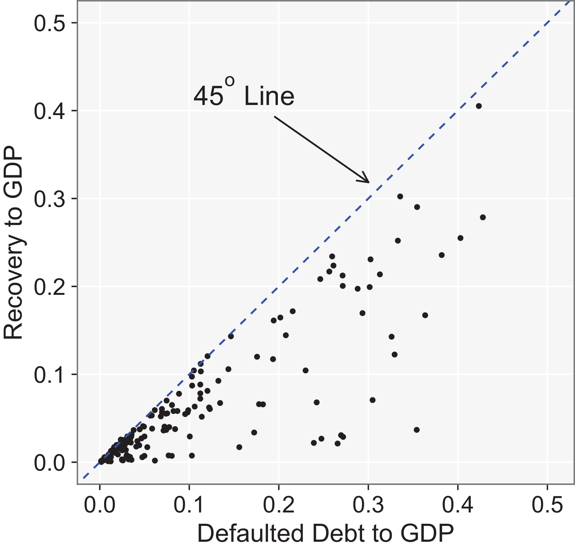
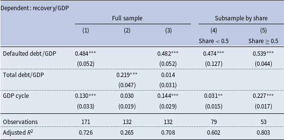
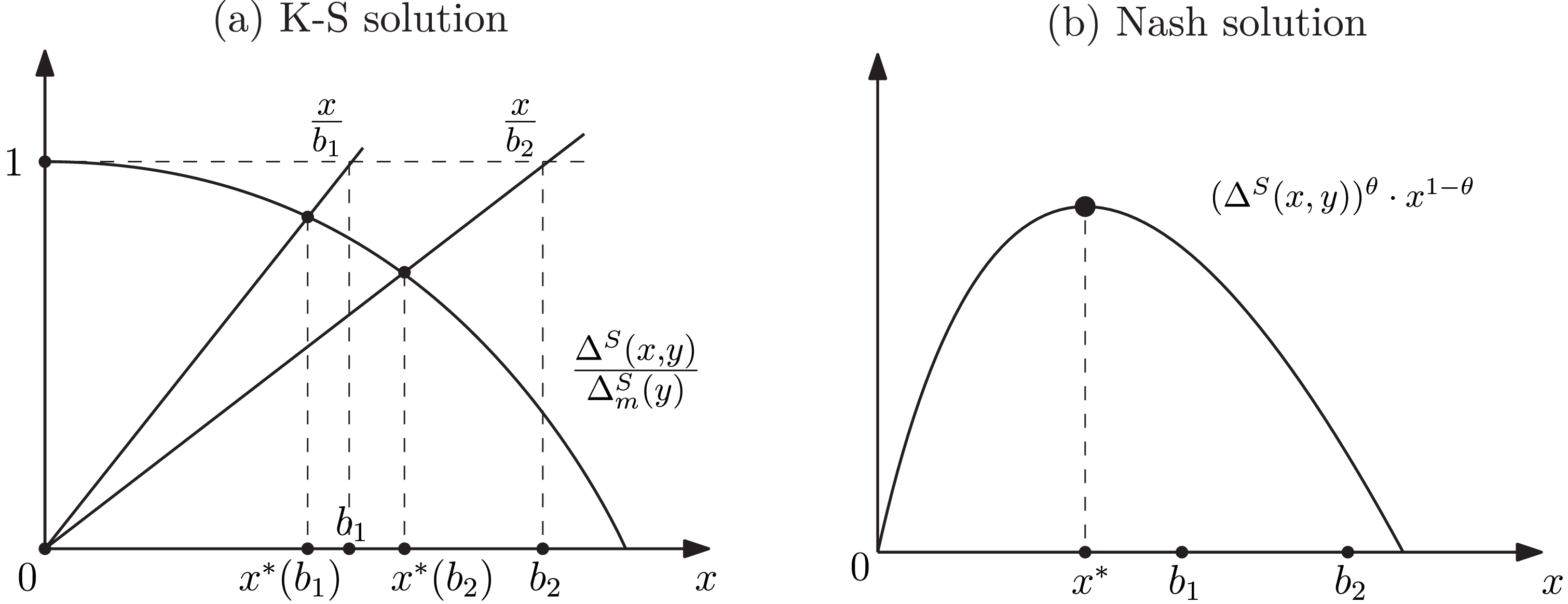
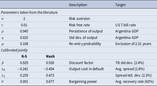
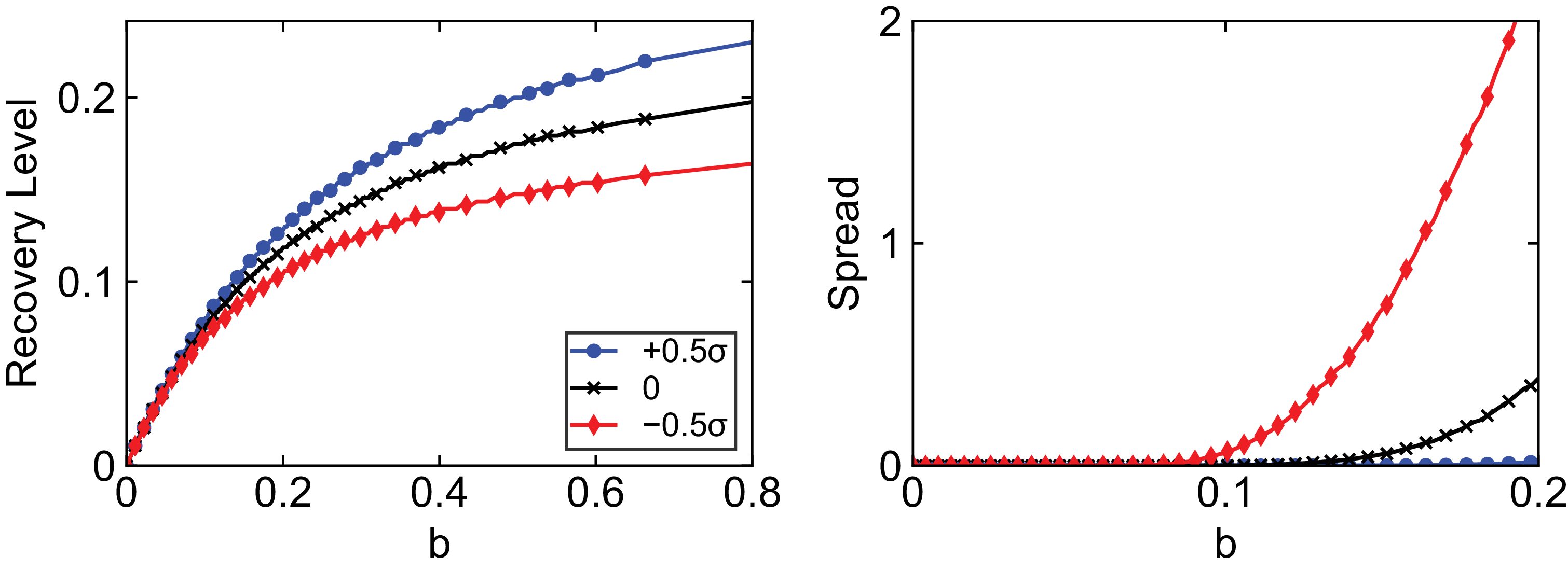
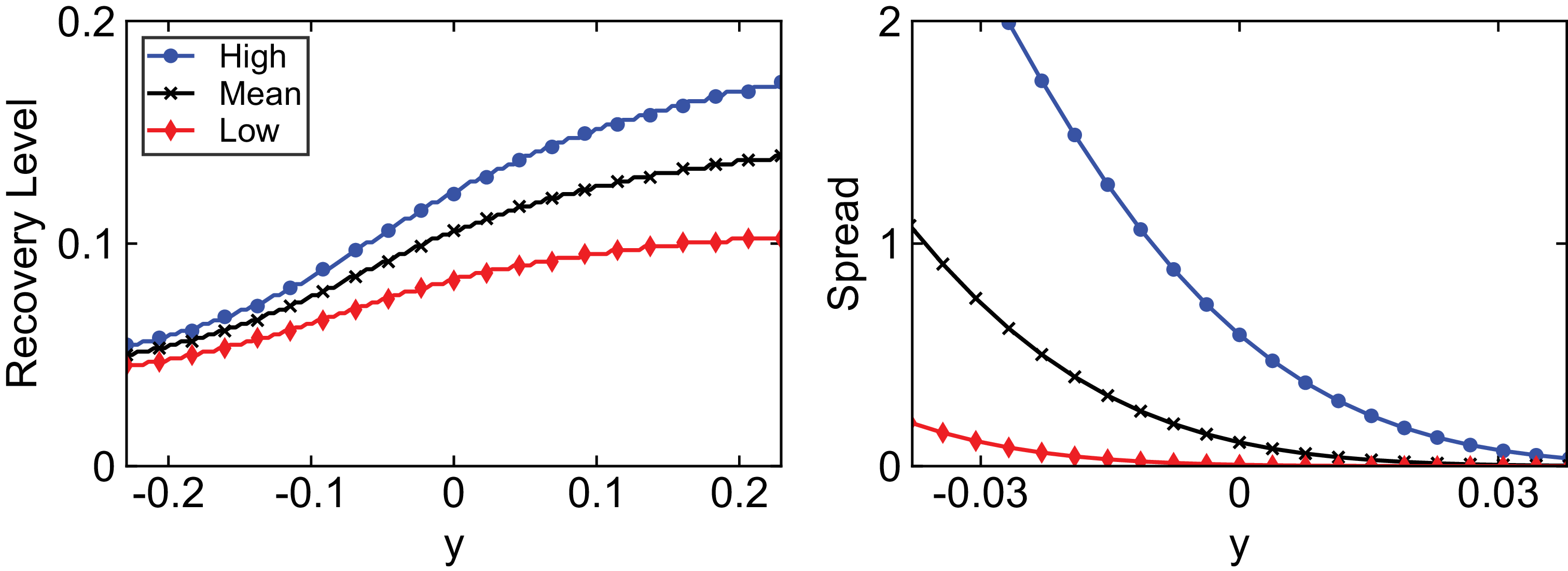

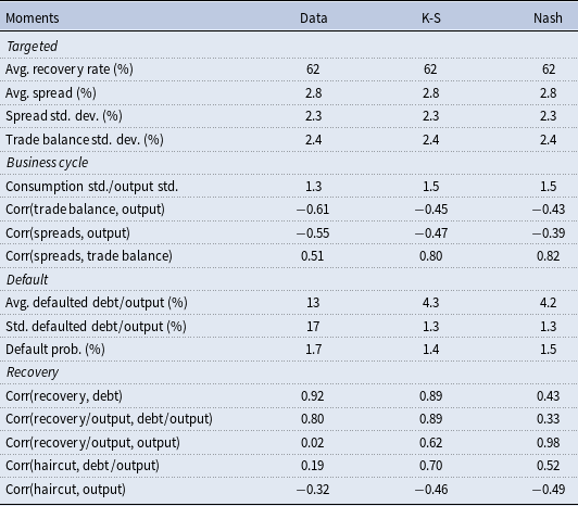

 45
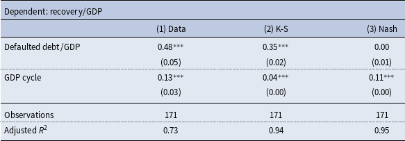
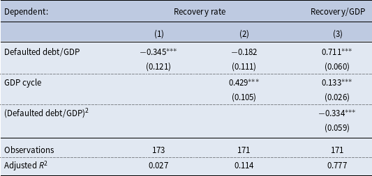
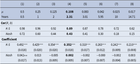
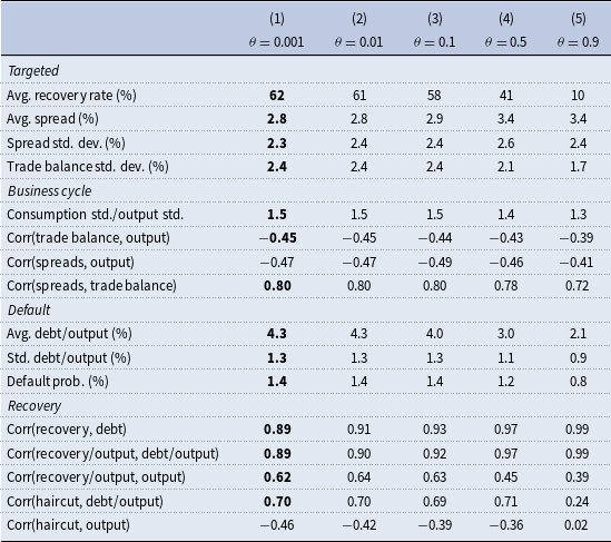
 θ
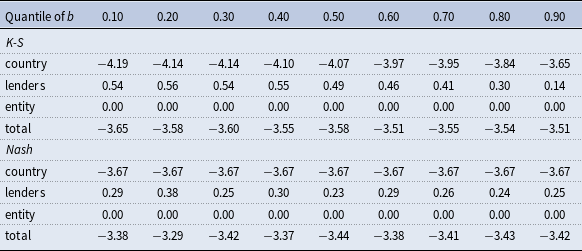
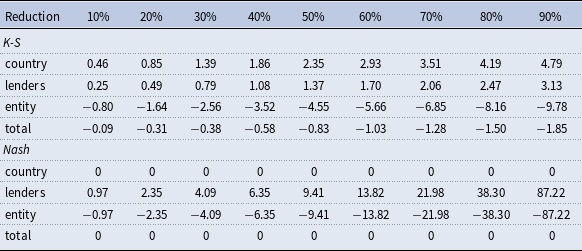
 %
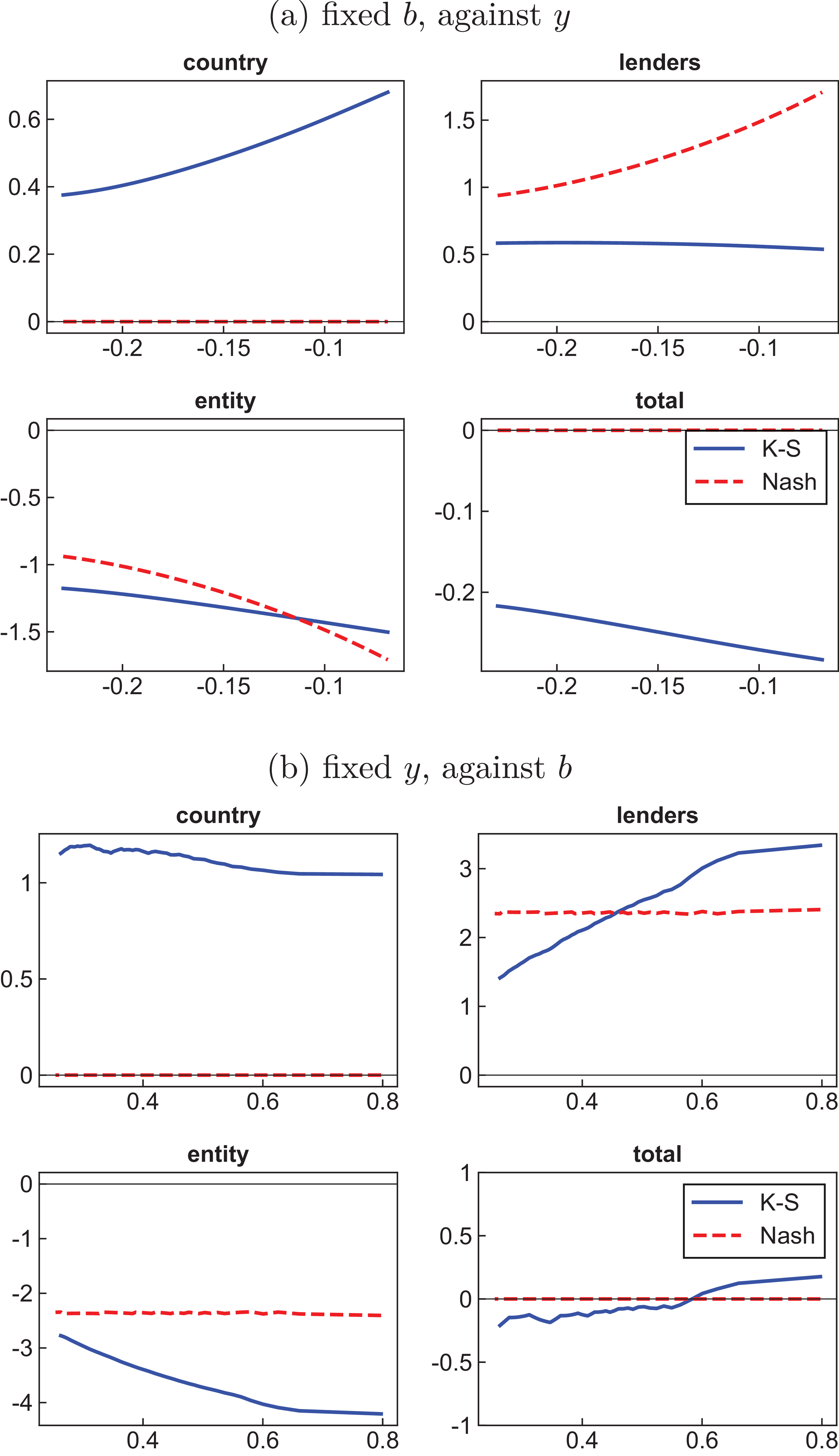
 %
 20%


